xDeepFM: Combining Explicit and Implicit Feature Interactions for Recommender Systems

Abstract.

Combinatorial features are essential for the success of many commercial models. Manually crafting these features usually comes with high cost due to the variety, volume and velocity of raw data in web-scale systems. Factorization based models, which measure interactions in terms of vector product, can learn patterns of combinatorial features automatically and generalize to unseen features as well. With the great success of deep neural networks (DNNs) in various fields, recently researchers have proposed several DNN-based factorization model to learn both low- and high-order feature interactions. Despite the powerful ability of learning an arbitrary function from data, plain DNNs generate feature interactions implicitly and at the bit-wise level. In this paper, we propose a novel Compressed Interaction Network (CIN), which aims to generate feature interactions in an explicit fashion and at the vector-wise level. We show that the CIN share some functionalities with convolutional neural networks (CNNs) and recurrent neural networks (RNNs). We further combine a CIN and a classical DNN into one unified model, and named this new model eXtreme Deep Factorization Machine (xDeepFM). On one hand, the xDeepFM is able to learn certain bounded-degree feature interactions explicitly; on the other hand, it can learn arbitrary low- and high-order feature interactions implicitly. We conduct comprehensive experiments on three real-world datasets. Our results demonstrate that xDeepFM outperforms state-of-the-art models. We have released the source code of xDeepFM at https://github.com/Leavingseason/xDeepFM.

1. introduction

Features play a central role in the success of many predictive systems. Because using raw features can rarely lead to optimal results, data scientists usually spend a lot of work on the transformation of raw features in order to generate best predictive systems (He et al., 2014; Lian et al., 2017c) or to win data mining games (Liu et al., 2016; Lian et al., 2017a; Lian and Xie, 2016). One major type of feature transformation is the cross-product transformation over categorical features (Cheng et al., 2016). These features are called cross features or multi-way features, they measure the interactions of multiple raw features. For instance, a 3-way feature AND(user_organization=msra, item_category=deeplearning, time=monday) has value 1 if the user works at Microsoft Research Asia and is shown a technical article about deep learning on a Monday.
There are three major downsides for traditional cross feature engineering. First, obtaining high-quality features comes with a high cost. Because right features are usually task-specific, data scientists need spend a lot of time exploring the potential patterns from the product data before they become domain experts and extract meaningful cross features. Second, in large-scale predictive systems such as web-scale recommender systems, the huge number of raw features makes it infeasible to extract all cross features manually. Third, hand-crafted cross features do not generalize to unseen interactions in the training data. Therefore, learning to interact features without manual engineering is a meaningful task.
Factorization Machines (FM) (Rendle, 2010) embed each feature $i$ to a latent factor vector $\mathbf{v}_{i}=[v_{i1},v_{i2},...,v_{iD}]$, and pairwise feature interactions are modeled as the inner product of latent vectors: $f^{(2)}(i,j)=\langle\mathbf{v}_{i},\mathbf{v}_{j}\rangle x_{i}x_{j}$. In this paper we use the term bit to denote a element (such as $v_{i1}$) in latent vectors. The classical FM can be extended to arbitrary higher-order feature interactions (Blondel et al., 2016), but one major downside is that, (Blondel et al., 2016) proposes to model all feature interactions, including both useful and useless combinations. As revealed in (Xiao et al., 2017), the interactions with useless features may introduce noises and degrade the performance. In recent years, deep neural networks (DNNs) have become successful in computer vision, speech recognition, and natural language processing with their great power of feature representation learning. It is promising to exploit DNNs to learn sophisticated and selective feature interactions. (Zhang et al., 2016a) proposes a Factorisation-machine supported Neural Network (FNN) to learn high-order feature interactions. It uses the pre-trained factorization machines for field embedding before applying DNN. (Qu et al., 2016) further proposes a Product-based Neural Network (PNN), which introduces a product layer between embedding layer and DNN layer, and does not rely on pre-trained FM. The major downside of FNN and PNN is that they focus more on high-order feature interactions while capture little low-order interactions. The Wide&Deep (Cheng et al., 2016) and DeepFM (Guo et al., 2017) models overcome this problem by introducing hybrid architectures, which contain a shallow component and a deep component with the purpose of learning both memorization and generalization. Therefore they can jointly learn low-order and high-order feature interactions.
All the abovementioned models leverage DNNs for learning high-order feature interactions. However, DNNs model high-order feature interactions in an implicit fashion. The final function learned by DNNs can be arbitrary, and there is no theoretical conclusion on what the maximum degree of feature interactions is. In addition, DNNs model feature interactions at the bit-wise level, which is different from the traditional FM framework which models feature interactions at the vector-wise level. Thus, in the field of recommender systems, whether DNNs are indeed the most effective model in representing high-order feature interactions remains an open question. In this paper, we propose a neural network-based model to learn feature interactions in an explicit, vector-wise fashion. Our approach is based on the Deep & Cross Network (DCN) (Wang et al., 2017), which aims to efficiently capture feature interactions of bounded degrees. However, we will argue in Section 2.3 that DCN will lead to a special format of interactions. We thus design a novel compressed interaction network (CIN) to replace the cross network in the DCN. CIN learns feature interactions explicitly, and the degree of interactions grows with the depth of the network. Following the spirit of the Wide&Deep and DeepFM models, we combine the explicit high-order interaction module with implicit interaction module and traditional FM module, and name the joint model eXtreme Deep Factorization Machine (xDeepFM). The new model requires no manual feature engineering and release data scientists from tedious feature searching work. To summarize, we make the following contributions:

• We propose a novel model, named eXtreme Deep Factorization Machine (xDeepFM), that jointly learns explicit and implicit high-order feature interactions effectively and requires no manual feature engineering.

• We design a compressed interaction network (CIN) in xDeepFM that learns high-order feature interactions explicitly. We show that the degree of feature interactions increases at each layer, and features interact at the vector-wise level rather than the bit-wise level.

• We conduct extensive experiments on three real-world dataset, and the results demonstrate that our xDeepFM outperforms several state-of-the-art models significantly.

The rest of this paper is organized as follows. Section 2 provides some preliminary knowledge which is necessary for understanding deep learning-based recommender systems. Section 3 introduces our proposed CIN and xDeepFM model in detail. We will present experimental explorations on multiple datasets in Section 4. Related works are discussed in Section 5. Section 6 concludes this paper.

2. Preliminaries

2.1. Embedding Layer

In computer vision or natural language understanding, the input data are usually images or textual signals, which are known to be spatially and/or temporally correlated, so DNNs can be applied directly on the raw feature with dense structures. However, in web-scale recommender systems, the input features are sparse, of huge dimension, and present no clear spatial or temporal correlation. Therefore, multi-field categorical form is widely used by related works (Guo et al., 2017; Shan et al., 2016; Wang et al., 2017; Qu et al., 2016; Zhang et al., 2016a). For example, one input instance [user_id=s02,gender=male,
organization=msra,interests=comedy&rock] is normally transformed into a high-dimensional sparse features via field-aware one-hot encoding:

$$[\underbrace{0,1,0,0,...,0}_{userid}]\ [\underbrace{1,0}_{gender}]\ [\underbrace{0,1,0,0,...,0}_{organization}]\ [\underbrace{0,1,0,1,...,0}_{interests}]$$

An embedding layer is applied upon the raw feature input to compress it to a low dimensional, dense real-value vector. If the field is univalent, the feature embedding is used as the field embedding. Take the above instance as an example, the embedding of feature male is taken as the embedding of field gender. If the field is multivalent, the sum of feature embedding is used as the field embedding. The embedding layer is illustrated in Figure 1. The result of embedding layer is a wide concatenated vector:

$$\mathbf{e}=[\mathbf{e}_{1},\mathbf{e}_{2},...,\mathbf{e}_{m}]$$

where $m$ denotes the number of fields, and $\mathbf{e_{i}}\in\mathbb{R}^{D}$ denotes the embedding of one field. Although the feature lengths of instances can be various, their embeddings are of the same length $m\times D$, where $D$ is the dimension of field embedding.

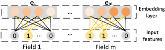
Figure 1. The field embedding layer. The dimension of embedding in this example is 4.

2.2. Implicit High-order Interactions

FNN (Zhang et al., 2016a), Deep Crossing (Shan et al., 2016), and the deep part in Wide&Deep (Cheng et al., 2016) exploit a feed-forward neural network on the field embedding vector $\mathbf{e}$ to learn high-order feature interactions. The forward process is :

(1) $$\mathbf{x}^{1}=\sigma(\mathbf{W}^{(1)}\mathbf{e}+\mathbf{b}^{1})$$

(2) $$\mathbf{x}^{k}=\sigma(\mathbf{W}^{(k)}\mathbf{x}^{(k-1)}+\mathbf{b}^{k})$$

where $k$ is the layer depth, $\sigma$ is an activation function, and $\mathbf{x}^{k}$ is the output of the $k$-th layer. The visual structure is very similar to what is shown in Figure 2, except that they do not include the FM or Product layer. This architecture models the interaction in a bit-wise fashion. That is to say, even the elements within the same field embedding vector will influence each other.
PNN (Qu et al., 2016) and DeepFM (Guo et al., 2017) modify the above architecture slightly. Besides applying DNNs on the embedding vector $\mathbf{e}$, they add a two-way interaction layer in the architecture. Therefore, both bit-wise and vector-wise interaction is included in their model. The major difference between PNN and DeepFM, is that PNN connects the outputs of product layer to the DNNs, whereas DeepFM connects the FM layer directly to the output unit (refer to Figure 2).

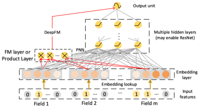
Figure 2. The architecture of DeepFM (with linear part omitted) and PNN. We re-use the symbols in (Guo et al., 2017), where red edges represent weight-1 connections (no parameters) and gray edges represent normal connections (network parameters).

2.3. Explicit High-order Interactions

(Wang et al., 2017) proposes the Cross Network (CrossNet) whose architecture is shown in Figure 3. It aims to explicitly model the high-order feature interactions. Unlike the classical fully-connected feed-forward network, the hidden layers are calculated by the following cross operation:

(3) $$\mathbf{x}_{k}=\mathbf{x}_{0}\mathbf{x}_{k-1}^{T}\mathbf{w}_{k}+\mathbf{b}_{k}+\mathbf{x}_{k-1}$$

where $\mathbf{w}_{k},\mathbf{b}_{k},\mathbf{x}_{k}\in\mathbb{R}^{mD}$ are weights, bias and output of the $k$-th layer, respectively. We argue that the CrossNet learns a special type of high-order feature interactions, where each hidden layer in the CrossNet is a scalar multiple of $\mathbf{x}_{0}$.

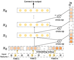
Figure 3. The architecture of the Cross Network.

Theorem 2.1.

Consider a $k$-layer cross network with the (i+1)-th layer defined as $\mathbf{x}_{i+1}=\mathbf{x}_{0}\mathbf{x}_{i}^{T}\mathbf{w}_{i+1}+\mathbf{x}_{i}$. Then, the output of the cross network $\mathbf{x}_{k}$ is a scalar multiple of $\mathbf{x}_{0}$.

Proof.

When $k$=1, according to the associative law and distributive law for matrix multiplication, we have:

(4) $$\begin{split}\mathbf{x}_{1}&=\mathbf{x}_{0}(\mathbf{x}_{0}^{T}\mathbf{w}_{1})+\mathbf{x}_{0}\\ &=\mathbf{x}_{0}(\mathbf{x}_{0}^{T}\mathbf{w}_{1}+1)\\ &=\alpha^{1}\mathbf{x}_{0}\end{split}$$

where the scalar $\alpha^{1}=\mathbf{x}_{0}^{T}\mathbf{w}_{1}+1$ is actually a linear regression of $\mathbf{x}_{0}$. Thus, $\mathbf{x}_{1}$ is a scalar multiple of $\mathbf{x}_{0}$. Suppose the scalar multiple statement holds for $k$=$i$. For $k$=$i+1$, we have :

(5) $$\begin{split}\mathbf{x}_{i+1}&=\mathbf{x}_{0}\mathbf{x}_{i}^{T}\mathbf{w}_{i+1}+\mathbf{x}_{i}\\ &=\mathbf{x}_{0}((\alpha^{i}\mathbf{x}_{0})^{T}\mathbf{w}_{i+1})+\alpha^{i}\mathbf{x}_{0}\\ &=\alpha^{i+1}\mathbf{x}_{0}\end{split}$$

where, $\alpha^{i+1}=\alpha^{i}(\mathbf{x}_{0}^{T}\mathbf{w}_{i+1}+1)$ is a scalar. Thus $\mathbf{x}_{i+1}$ is still a scalar multiple of $\mathbf{x}_{0}$. By induction hypothesis, the output of cross network $\mathbf{x}_{k}$ is a scalar multiple of $\mathbf{x}_{0}$. ∎

Note that the scalar multiple does not mean $\mathbf{x}_{k}$ is linear with $\mathbf{x}_{0}$. The coefficient $\alpha^{i+1}$ is sensitive with $\mathbf{x}_{0}$. The CrossNet can learn feature interactions very efficiently (the complexity is negligible compared with a DNN model), however the downsides are: (1) the output of CrossNet is limited in a special form, with each hidden layer is a scalar multiple of $\mathbf{x}_{0}$; (2) interactions come in a bit-wise fashion.

3. Our proposed model

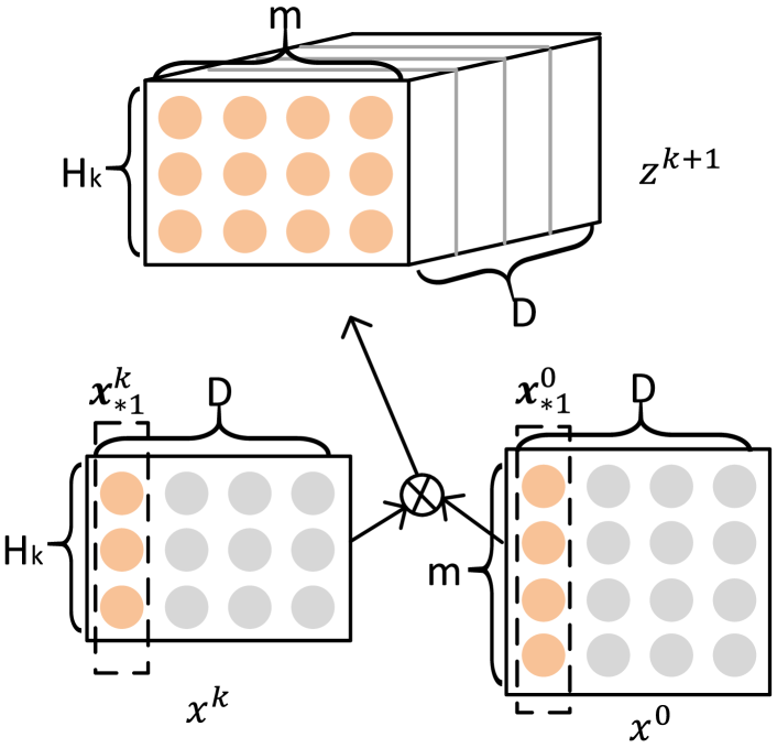
(a) Outer products along each dimension for feature interactions. The tensor $\mathbf{Z}^{k+1}$ is an intermediate result for further learning.

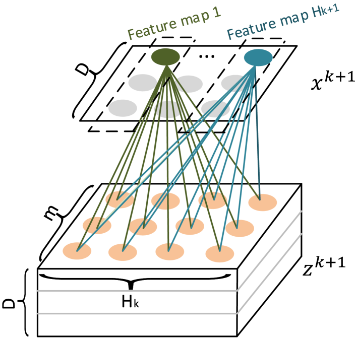
(b) The $k$-th layer of CIN. It compresses the intermediate tensor $\mathbf{Z}^{k+1}$ to $H_{k+1}$ embedding vectors (aslo known as feature maps).

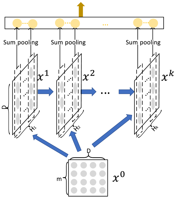
(c) An overview of the CIN architecture.

Figure 4. Components and architecture of the Compressed Interaction Network (CIN).

3.1. Compressed Interaction Network

We design a new cross network, named Compressed Interaction Network (CIN), with the following considerations: (1) interactions are applied at vector-wise level, not at bit-wise level; (2) high-order feature interactions is measured explicitly; (3) the complexity of network will not grow exponentially with the degree of interactions.
Since an embedding vector is regarded as a unit for vector-wise interactions, hereafter we formulate the output of field embedding as a matrix $\mathbf{X}^{0}\in\mathbb{R}^{m\times D}$, where the $i$-th row in $\mathbf{X}^{0}$ is the embedding vector of the $i$-th field: $\mathbf{X}^{0}_{i,*}=\mathbf{e}_{i}$, and $D$ is the dimension of the field embedding. The output of the $k$-th layer in CIN is also a matrix $\mathbf{X}^{k}\in\mathbb{R}^{H_{k}\times D}$, where $H_{k}$ denotes the number of (embedding) feature vectors in the $k$-th layer and we let $H_{0}=m$. For each layer, $\mathbf{X}^{k}$ are calculated via:

(6) $$\mathbf{X}^{k}_{h,*}=\sum_{i=1}^{H_{k-1}}\sum_{j=1}^{m}\mathbf{W}^{k,h}_{ij}(\mathbf{X}^{k-1}_{i,*}\circ\mathbf{X}^{0}_{j,*})$$

where $1\leq h\leq H_{k}$, $\mathbf{W}^{k,h}\in\mathbb{R}^{H_{k-1}\times m}$ is the parameter matrix for the $h$-th feature vector, and $\circ$ denotes the Hadamard product, for example, $\langle a_{1},a_{2},a_{3}\rangle\circ\langle b_{1},b_{2},b_{3}\rangle=\langle a_{1}b_{1},a_{2}b_{2},a_{3}b_{3}\rangle$. Note that $\mathbf{X}^{k}$ is derived via the interactions between $\mathbf{X}^{k-1}$ and $\mathbf{X}^{0}$, thus feature interactions are measured explicitly and the degree of interactions increases with the layer depth. The structure of CIN is very similar to the Recurrent Neural Network (RNN), where the outputs of the next hidden layer are dependent on the last hidden layer and an additional input. We hold the structure of embedding vectors at all layers, thus the interactions are applied at the vector-wise level.
It is interesting to point out that Equation 6 has strong connections with the well-known Convolutional Neural Networks (CNNs) in computer vision. As shown in Figure 4(a), we introduce an intermediate tensor $\mathbf{Z}^{k+1}$, which is the outer products (along each embedding dimension) of hidden layer $\mathbf{X}^{k}$ and original feature matrix $\mathbf{X}^{0}$. Then $\mathbf{Z}^{k+1}$ can be regarded as a special type of image and $\mathbf{W}^{k,h}$ is a filter. We slide the filter across $\mathbf{Z}^{k+1}$ along the embedding dimension (D) as shown in Figure 4(b), and get an hidden vector $\mathbf{X}^{k+1}_{i,*}$, which is usually called a feature map in computer vision. Therefore, $\mathbf{X}^{k}$ is a collection of $H_{k}$ different feature maps. The term “compressed” in the name of CIN indicates that the $k$-th hidden layer compress the potential space of $H_{k-1}\times m$ vectors down to $H_{k}$ vectors.
Figure 4(c) provides an overview of the architecture of CIN. Let T denotes the depth of the network. Every hidden layer $\mathbf{X}^{k},k\in[1,T]$ has a connection with output units. We first apply sum pooling on each feature map of the hidden layer:

(7) $${p}^{k}_{i}=\sum_{j=1}^{D}\mathbf{X}^{k}_{i,j}$$

for $i\in[1,H_{k}]$. Thus, we have a pooling vector $\mathbf{p}^{k}=[p^{k}_{1},p^{k}_{2},...,p^{k}_{H_{k}}]$ with length $H_{k}$ for the $k$-th hidden layer. All pooling vectors from hidden layers are concatenated before connected to output units: $\mathbf{p}^{+}=[\mathbf{p}^{1},\mathbf{p}^{2},...,\mathbf{p}^{T}]\in\mathbb{R}^{\sum_{i=1}^{T}H_{i}}$. If we use CIN directly for binary classification, the output unit is a sigmoid node on $\mathbf{p}^{+}$:

(8) $$y=\frac{1}{1+exp(\mathbf{p^{+}}^{T}\mathbf{w}^{o})}$$

where $\mathbf{w}^{o}$ are the regression parameters.

3.2. CIN Analysis

We analyze the proposed CIN to study the model complexity and the potential effectiveness.

3.2.1. Space Complexity

The $h$-th feature map at the $k$-th layer contains $H_{k-1}\times m$ parameters, which is exactly the size of $\mathbf{W}^{k,h}$. Thus, there are $H_{k}\times H_{k-1}\times m$ parameters at the $k$-th layer. Considering the last regression layer for the output unit, which has $\sum_{k=1}^{T}H_{k}$ parameters, the total number of parameters for CIN is $\sum_{k=1}^{T}H_{k}\times(1+H_{k-1}\times m)$. Note that CIN is independent of the embedding dimension $D$. In contrast, a plain $T$-layers DNN contains $m\times D\times H_{1}+H_{T}+\sum_{k=2}^{T}H_{k}\times H_{k-1}$ parameters, and the number of parameters will increase with the embedding dimension $D$.
Usually $m$ and $H_{k}$ will not be very large, so the scale of $\mathbf{W}^{k,h}$ is acceptable. When necessary, we can exploit a $L$-order decomposition and replace $\mathbf{W}^{k,h}$ with two smaller matrices $\mathbf{U}^{k,h}\in\mathbb{R}^{H_{k-1}\times L}$ and $\mathbf{V}^{k,h}\in\mathbb{R}^{m\times L}$:

(9) $$\mathbf{W}^{k,h}=\mathbf{U}^{k,h}(\mathbf{V}^{k,h})^{T}$$

where $L\ll H$ and $L\ll m$. Hereafter we assume that each hidden layer has the same number (which is $H$) of feature maps for simplicity. Through the $L$-order decomposition, the space complexity of CIN is reduced from $O(mTH^{2})$ to $O(mTHL+TH^{2}L)$. In contrast, the space complexity of the plain DNN is $O(mDH+TH^{2})$, which is sensitive to the dimension (D) of field embedding.

3.2.2. Time Complexity

The cost of computing tensor $\mathbf{Z}^{k+1}$ (as shown in Figure 4(a)) is $O(mHD)$ time. Because we have $H$ feature maps in one hidden layer, computing a $T$-layers CIN takes $O(mH^{2}DT)$ time. A $T$-layers plain DNN, by contrast, takes $O(mHD+H^{2}T)$ time. Therefore, the major downside of CIN lies in the time complexity.

3.2.3. Polynomial Approximation

Next we examine the high-order interaction properties of CIN. For simplicity, we assume that numbers of feature maps at hidden layers are all equal to the number of fields $m$. Let $[m]$ denote the set of positive integers that are less than or equal to $m$. The $h$-th feature map at the first layer, denoted as $\mathbf{x}^{1}_{h}\ \in\mathbb{R}^{D}$, is calculated via:

(10) $$\mathbf{x}^{1}_{h}=\sum_{\begin{subarray}{c}i\in[m]\\ j\in[m]\end{subarray}}\mathbf{W}^{1,h}_{i,j}(\mathbf{x}^{0}_{i}\circ\mathbf{x}^{0}_{j})$$

Therefore, each feature map at the first layer models pair-wise interactions with $O(m^{2})$ coefficients. Similarly, the $h$-th feature map at the second layer is:

(11) $$\begin{split}\mathbf{x}^{2}_{h}&=\sum_{\begin{subarray}{c}i\in[m]\\ j\in[m]\end{subarray}}\mathbf{W}^{2,h}_{i,j}(\mathbf{x}^{1}_{i}\circ\mathbf{x}^{0}_{j})\\ &=\sum_{\begin{subarray}{c}i\in[m]\\ j\in[m]\end{subarray}}\sum_{\begin{subarray}{c}l\in[m]\\ k\in[m]\end{subarray}}\mathbf{W}^{2,h}_{i,j}\mathbf{W}^{1,i}_{l,k}(\mathbf{x}^{0}_{j}\circ\mathbf{x}^{0}_{k}\circ\mathbf{x}^{0}_{l})\end{split}$$

Note that all calculations related to the subscript $l$ and $k$ is already finished at the previous hidden layer. We expand the factors in Equation 11 just for clarity. We can observe that each feature map at the second layer models 3-way interactions with $O(m^{2})$ new parameters.
A classical $k$-order polynomial has $O(m^{k})$ coefficients. We show that CIN approximate this class of polynomial with only $O(km^{3})$ parameters in terms of a chain of feature maps. By induction hypothesis, we can prove that the $h$-th feature map at the $k$-th layer is:

(12) $$\begin{split}\mathbf{x}^{k}_{h}&=\sum_{\begin{subarray}{c}i\in[m]\\ j\in[m]\end{subarray}}\mathbf{W}^{k,h}_{i,j}(\mathbf{x}^{k-1}_{i}\circ\mathbf{x}^{0}_{j})\\ &=\sum_{\begin{subarray}{c}i\in[m]\\ j\in[m]\end{subarray}}...\sum_{\begin{subarray}{c}r\in[m]\\ t\in[m]\end{subarray}}\sum_{\begin{subarray}{c}l\in[m]\\ s\in[m]\end{subarray}}\mathbf{W}^{k,h}_{i,j}...\mathbf{W}^{1,r}_{l,s}(\underbrace{\mathbf{x}^{0}_{j}\circ...\circ\mathbf{x}^{0}_{s}\circ\mathbf{x}^{0}_{l}}_{k\ vectors})\end{split}$$

For better illustration, here we borrow the notations from (Wang et al., 2017). Let $\boldsymbol{\alpha}=[\alpha_{1},...,\alpha_{m}]\in\mathbb{N}^{d}$ denote a multi-index, and $|\boldsymbol{\alpha}|=\sum_{i=1}^{m}\alpha_{i}$. We omit the original superscript from $\mathbf{x}^{0}_{i}$, and use $\mathbf{x}_{i}$ to denote it since we only we the feature maps from the $0$-th layer (which is exactly the field embeddings) for the final expanded expression (refer to Eq. 12). Now a superscript is used to denote the vector operation, such as $\mathbf{x}^{3}_{i}=\mathbf{x}_{i}\circ\mathbf{x}_{i}\circ\mathbf{x}_{i}$. Let $VP_{k}(\mathbf{X})$ denote a multi-vector polynomial of degree $k$:

(13) $$VP_{k}(\mathbf{X})=\left\{\left.\sum_{\boldsymbol{\alpha}}w_{\boldsymbol{\alpha}}\mathbf{x}_{1}^{\alpha_{1}}\circ\mathbf{x}_{2}^{\alpha_{2}}\circ...\circ\mathbf{x}_{m}^{\alpha_{m}}\right|2\leqslant|\boldsymbol{\alpha}|\leqslant k\right\}$$

Each vector polylnomial in this class has $O(m^{k})$ coefficients. Then, our CIN approaches the coefficient $w_{\boldsymbol{\alpha}}$ with:

(14) $$\hat{w}_{\boldsymbol{\alpha}}=\sum_{i=1}^{m}\sum_{j=1}^{m}\sum_{B\in P_{\boldsymbol{\alpha}}}\prod_{t=2}^{|\boldsymbol{\alpha}|}\mathbf{W}^{t,j}_{i,B_{t}}$$

where, $B=[B_{1},B_{2},...,B_{|\boldsymbol{\alpha}|}]$ is a multi-index, and $P_{\boldsymbol{\alpha}}$ is the set of all the permutations of the indices $(\underbrace{1,...1}_{\alpha_{1}\ times},...,\underbrace{m,...,m}_{\alpha_{m}\ times})$.

3.3. Combination with Implicit Networks

As discussed in Section 2.2, plain DNNs learn implicit high-order feature interactions. Since CIN and plain DNNs can complement each other, an intuitive way to make the model stronger is to combine these two structures. The resulting model is very similar to the Wide&Deep or DeepFM model. The architecture is shown in Figure 5. We name the new model eXtreme Deep Factorization Machine (xDeepFM), considering that on one hand, it includes both low-order and high-order feature interactions; on the other hand, it includes both implicit feature interactions and explicit feature interactions. Its resulting output unit becomes:

(15) $$\hat{y}=\sigma(\mathbf{w}_{linear}^{T}\mathbf{a}+\mathbf{w}^{T}_{dnn}\mathbf{x}^{k}_{dnn}+\mathbf{w}^{T}_{cin}\mathbf{p}^{+}+b)$$

where $\sigma$ is the sigmoid function, $\mathbf{a}$ is the raw features. $\mathbf{x}^{k}_{dnn},\mathbf{p}^{+}$ are the outputs of the plain DNN and CIN, respectively. $\mathbf{w}_{*}$ and $b$ are learnable parameters. For binary classifications, the loss function is the log loss:

(16) $$\mathcal{L}=-\frac{1}{N}\sum_{i=1}^{N}y_{i}log\hat{y}_{i}+(1-y_{i})log(1-\hat{y}_{i})$$

where $N$ is the total number of training instances. The optimization process is to minimize the following objective function:

(17) $$\mathcal{J}=\mathcal{L}+\lambda_{*}||\Theta||$$

where $\lambda_{*}$ denotes the regularization term and $\Theta$ denotes the set of parameters, including these in linear part, CIN part, and DNN part.

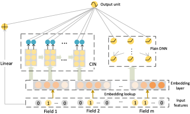
Figure 5. The architecture of xDeepFM.

3.3.1. Relationship with FM and DeepFM

Suppose all fields are univalent. It’s not hard to observe from Figure 5 that, when the depth and feature maps of the CIN part are both set to 1, xDeepFM is a generalization of DeepFM by learning the linear regression weights for the FM layer (note that in DeepFM, units of FM layer are directly linked to the output unit without any coefficients). When we further remove the DNN part, and at the same time use a constant sum filter (which simply takes the sum of inputs without any parameter learning) for the feature map, then xDeepFM is downgraded to the traditional FM model.

4. Experiments

In this section, we conduct extensive experiments to answer the following questions:

• (Q1) How does our proposed CIN perform in high-order feature interactions learning?

• (Q2) Is it necessary to combine explicit and implicit high-order feature interactions for recommender systems?

• (Q3) How does the settings of networks influence the performance of xDeepFM?

We will answer these questions after presenting some fundamental experimental settings.

4.1. Experiment Setup

4.1.1. Datasets.

We evaluate our proposed models on the following three datasets:
1. Criteo Dataset. It is a famous industry benchmarking dataset for developing models predicting ad click-through rate, and is publicly accessible. Given a user and the page he is visiting, the goal is to predict the probability that he will clik on a given ad.
2. Dianping Dataset. Dianping.com is the largest consumer review site in China. It provides diverse functions such as reviews, check-ins, and shops’ meta information (including geographical messages and shop attributes). We collect 6 months’ users check-in activities for restaurant recommendation experiments. Given a user’s profile, a restaurant’s attributes and the user’s last three visited POIs (point of interest), we want to predict the probability that he will visit the restaurant. For each restaurant in a user’s check-in instance, we sample four restaurants which are within 3 kilometers as negative instances by POI popularity.
3. Bing News Dataset. Bing News is part of Microsoft’s Bing search engine. In order to evaluate the performance of our model in a real commercial dataset, we collect five consecutive days’ impression logs on news reading service. We use the first three days’ data for training and validation, and the next two days for testing.
For the Criteo dataset and the Dianping dataset, we randomly split instances by 8:1:1 for training , validation and test. The characteristics of the three datasets are summarized in Table 1.

Table 1. Statistics of the evaluation datasets. M indicates million and K indicates thousand.

Datasest	#instances	#fields	#features (sparse)
Criteo	45M	39	2.3M
Dianping	1.2M	18	230K
Bing News	5M	45	17K

4.1.2. Evaluation Metrics.

We use two metrics for model evaluation: AUC (Area Under the ROC curve) and Logloss (cross entropy). These two metrics evaluate the performance from two different angels: AUC measures the probability that a positive instance will be ranked higher than a randomly chosen negative one. It only takes into account the order of predicted instances and is insensitive to class imbalance problem. Logloss, in contrast, measures the distance between the predicted score and the true label for each instance. Sometimes we rely more on Logloss because we need to use the predicted probability to estimate the benefit of a ranking strategy (which is usually adjusted as CTR $\times$ bid).

4.1.3. Baselines.

We compare our xDeepFM with LR(logistic regression), FM, DNN (plain deep neural network), PNN (choose the better one from iPNN and oPNN) (Qu et al., 2016), Wide & Deep (Cheng et al., 2016), DCN (Deep & Cross Network) (Wang et al., 2017) and DeepFM (Guo et al., 2017). As introduced and discussed in Section 2, these models are highly related to our xDeepFM and some of them are state-of-the-art models for recommender systems. Note that the focus of this paper is to learn feature interactions automatically, so we do not include any hand-crafted cross features.

4.1.4. Reproducibility

We implement our method using Tensorflow. Hyper-parameters of each model are tuned by grid-searching on the validation set, and the best settings for each model will be shown in corresponding sections. Learning rate is set to 0.001. For optimization method, we use the Adam (Kingma and Ba, 2014) with a mini-batch size of 4096. We use a L2 regularization with $\lambda=0.0001$ for DNN, DCN, Wide&Deep, DeepFM and xDeepFM, and use dropout 0.5 for PNN. The default setting for number of neurons per layer is: (1) 400 for DNN layers; (2) 200 for CIN layers on Criteo dataset, and 100 for CIN layers on Dianping and Bing News datasets. Since we focus on neural networks structures in this paper, we make the dimension of field embedding for all models be a fixed value of 10. We conduct experiments of different settings in parallel with 5 Tesla K80 GPUs. The source code is available at https://github.com/Leavingseason/xDeepFM.

Table 2. Performance of individual models on the Criteo, Dianping, and Bing News datasets. Column Depth indicates the best network depth for each model.

Model name	AUC	Logloss	Depth
Criteo
FM	0.7900	0.4592	-
DNN	0.7993	0.4491	2
CrossNet	0.7961	0.4508	3
CIN	0.8012	0.4493	3
Dianping
FM	0.8165	0.3558	-
DNN	0.8318	0.3382	3
CrossNet	0.8283	0.3404	2
CIN	0.8576	0.3225	2
Bing News
FM	0.8223	0.2779	-
DNN	0.8366	0.273	2
CrossNet	0.8304	0.2765	6
CIN	0.8377	0.2662	5

Table 3. Overall performance of different models on Criteo, Dianping and Bing News datasets. The column Depth presents the best setting for network depth with a format of (cross layers, DNN layers).

	Criteo			Dianping			Bing News
Model name	AUC	Logloss	Depth	AUC	Logloss	Depth	AUC	Logloss	Depth
LR	0.7577	0.4854	-,-	0.8018	0.3608	-,-	0.7988	0.2950	-,-
FM	0.7900	0.4592	-,-	0.8165	0.3558	-,-	0.8223	0.2779	-,-
DNN	0.7993	0.4491	-,2	0.8318	0.3382	-,3	0.8366	0.2730	-,2
DCN	0.8026	0.4467	2,2	0.8391	0.3379	4,3	0.8379	0.2677	2,2
Wide&Deep	0.8000	0.4490	-,3	0.8361	0.3364	-,2	0.8377	0.2668	-,2
PNN	0.8038	0.4927	-,2	0.8445	0.3424	-,3	0.8321	0.2775	-,3
DeepFM	0.8025	0.4468	-,2	0.8481	0.3333	-,2	0.8376	0.2671	-,3
xDeepFM	0.8052	0.4418	3,2	0.8639	0.3156	3,3	0.8400	0.2649	3,2

4.2. Performance Comparison among Individual Neural Components (Q1)

We want to know how CIN performs individually. Note that FM measures 2-order feature interactions explicitly, DNN model high-order feature interactions implicitly, CrossNet tries to model high-order feature interactions with a small number of parameters (which is proven not effective in Section 2.3), and CIN models high-order feature interactions explicitly. There is no theoretic guarantee of the superiority of one individual model over the others, due to that it really depends on the dataset. For example, if the practical dataset does not require high-order feature interactions, FM may be the best individual model. Thus we do not have any expectation for which model will perform the best in this experiment.

Table 2 shows the results of individual models on the three practical datasets. Surprisingly, our CIN outperform the other models consistently. On one hand, the results indicate that for practical datasets, higher-order interactions over sparse features are necessary, and this can be verified through the fact that DNN, CrossNet and CIN outperform FM significantly on all the three datasets. On the other hand, CIN is the best individual model, which demonstrates the effectiveness of CIN on modeling explicit high-order feature interactions. Note that a $k$-layer CIN can model $k$-degree feature interactions. It is also interesting to see that it take 5 layers for CIN to yield the best result ON the Bing News dataset.

4.3. Performance of Integrated Models (Q2)

xDeepFM integrates CIN and DNN into an end-to-end model. While CIN and DNN covers two distinct properties in learning feature interactions, we are interested to know whether it is indeed necessary and effective to combine them together for jointly explicit and implicit learning. Here we compare several strong baselines which are not limited to individual models, and the results are shown in Table 3. We observe that LR is far worse than all the rest models, which demonstrates that factorization-based models are essential for measuring sparse features. Wide&Deep, DCN, DeepFM and xDeepFM are significantly better than DNN, which directly reflects that, despite their simplicity, incorporating hybrid components are important for boosting the accuracy of predictive systems. Our proposed xDeepFM achieves the best performance on all datasets, which demonstrates that combining explicit and implicit high-order feature interaction is necessary, and xDeepFM is effective in learning this class of combination. Another interesting observation is that, all the neural-based models do not require a very deep network structure for the best performance. Typical settings for the depth hyper-parameter are 2 and 3, and the best depth setting for xDeepFM is 3, which indicates that the interactions we learned are at most 4-order.

4.4. Hyper-Parameter Study (Q3)

We study the impact of hyper-parameters on xDeepFM in this section, including (1) the number of hidden layers; (2) the number of neurons per layer; and (3) activation functions. We conduct experiments via holding the best settings for the DNN part while varying the settings for the CIN part.

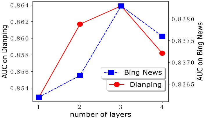
(a) Number of layers.

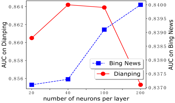
(b) Number of neurons per layer.

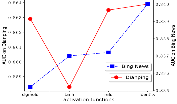
(c) Activation functions

Figure 6. Impact of network hyper-parameters on AUC performance.

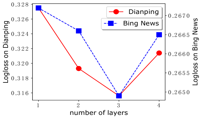
(a) Number of layers.

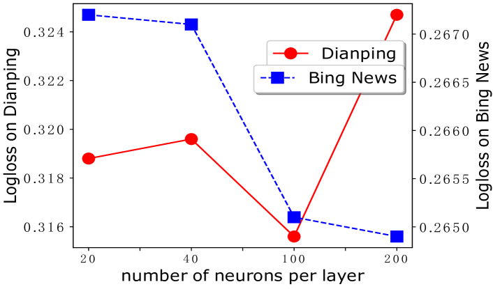
(b) Number of neurons per layer.

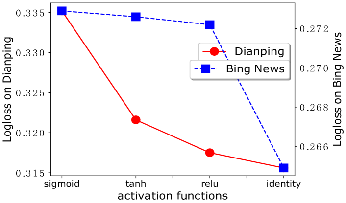
(c) Activation functions

Figure 7. Impact of network hyper-parameters on Logloss performance.

Depth of Network. Figure 6(a) and 7(a) demonstrate the impact of number of hidden layers. We can observe that the performance of xDeepFM increases with the depth of network at the beginning. However, model performance degrades when the depth of network is set greater than 3. It is caused by overfitting evidenced by that we notice that the loss of training data still keeps decreasing when we add more hidden layers.
Number of Neurons per Layer. Adding the number of neurons per layer indicates increasing the number of feature maps in CIN. As shown in Figure 6(b) and 7(b), model performance on Bing News dataset increases steadily when we increase the number of neurons from $20$ to $200$, while on Dianping dataset, $100$ is a more suitable setting for the number of neurons per layer. In this experiment we fix the depth of network at 3.
Activation Function. Note that we exploit the identity as activation function on neurons of CIN, as shown in Eq. 6. A common practice in deep learning literature is to employ non-linear activation functions on hidden neurons. We thus compare the results of different activation functions on CIN (for neurons in DNN, we keep the activation function with relu). As shown in Figure 6(c) and 7(c), identify function is indeed the most suitable one for neurons in CIN.

5. related work

5.1. Classical Recommender Systems

5.1.1. Non-factorization Models

For web-scale recommender systems (RSs), the input features are usually sparse, categorical-continuous-mixed, and high-dimensional. Linear models, such as logistic regression with FTRL (McMahan et al., 2013), are widely adopted as they are easy to manage, maintain, and deploy. Because linear models lack the ability of learning feature interactions, data scientists have to spend a lot of work on engineering cross features in order to achieve better performance (Richardson et al., 2007; Lian et al., 2017a). Considering that some hidden features are hard to design manually, some researchers exploit boosting decision trees to help build feature transformations (He et al., 2014; Ling et al., 2017).

5.1.2. Factorization Models

A major downside of the aforementioned models is that they can not generalize to unseen feature interactions in the training set. Factorization Machines (Rendle, 2010) overcome this problem via embedding each feature into a low dimension latent vector. Matrix factorization (MF) (Koren et al., 2009), which only considers IDs as features, can be regarded as a special kind of FM. Recommendations are made via the product of two latent vectors, thus it does not require the co-occurrence of user and item in the training set. MF is the most popular model-based collaborative filtering method in the RS literature (Srebro et al., 2005; Koren, 2008; Lee et al., 2013; Pan et al., 2008). (Chen et al., 2012; Menon and Elkan, 2010) extend MF to leveraging side information, in which both a linear model and a MF model are included. On the other hand, for many recommender systems, only implicit feedback datasets such as users’ watching history and browsing activities are available. Thus researchers extend the factorization models to a Bayesian Personalized Ranking (BPR) framework (Rendle et al., 2009; Rendle and Schmidt-Thieme, 2010; He and McAuley, 2016; Yuan et al., 2016) for implicit feedback.

5.2. Recommender Systems with Deep Learning

Deep learning techniques have achieved great success in computer vision (Krizhevsky et al., 2012; He et al., 2016), speech recognition (Hinton et al., 2012; Amodei et al., 2016) and natural language understanding (Mikolov et al., 2010; Cho et al., 2014). As a result, an increasing number of researchers are interested in employing DNNs for recommender systems.

5.2.1. Deep Learning for High-Order Interactions

To avoid manually building up high-order cross features, researchers apply DNNs on field embedding, thus patterns from categorical feature interactions can be learned automatically. Representative models include FNN (Zhang et al., 2016a), PNN (Qu et al., 2016), DeepCross (Shan et al., 2016), NFM (He and Chua, 2017), DCN (Wang et al., 2017), Wide&Deep (Cheng et al., 2016), and DeepFM (Guo et al., 2017). These models are highly related to our proposed xDeepFM. Since we have reviewed them in Section 1 and Section 2, we do not further discuss them in detail in this section. We have demonstrated that our proposed xDeepFM has two special properties in comparison with these models: (1) xDeepFM learns high-order feature interactions in both explicit and implicit fashions; (2) xDeepFM learns feature interactions at the vector-wise level rather than at the bit-wise level.

5.2.2. Deep Learning for Elaborate Representation Learning

We include some other deep learning-based RSs in this section due to that they are less focused on learning feature interactions. Some early work employs deep learning mainly to model auxiliary information, such as visual data (He and McAuley, 2016) and audio data (Wang and Wang, 2014). Recently, deep neural networks are used to model the collaborative filtering (CF) in RSs. (He et al., 2017) proposes a Neural Collaborative Filtering (NCF) so that the inner product in MF can be replaced with an arbitrary function via a neural architecture. (Sedhain et al., 2015; Wu et al., 2016) model CF base on the autoencoder paradigm, and they have empirically demonstrated that autoencoder-based CF outperforms several classical MF models. Autoencoders can be further employed for jointly modeling CF and side information with the purpose of generating better latent factors (Dong et al., 2017; Wang et al., 2015; Zhang et al., 2016b). (Elkahky et al., 2015; Lian et al., 2017b) employ neural networks to jointly train multiple domains’ latent factors. (Chen et al., 2017) proposes the Attentive Collaborative Filtering (ACF) to learn more elaborate preference at both item-level and component-level. (Zhou et al., 2017) shows tha traditional RSs can not capture interest diversity and local activation effectively, so they introduce a Deep Interest Network (DIN) to represent users’ diverse interests with an attentive activation mechanism.

6. Conclusions

In this paper, we propose a novel network named Compressed Interaction Network (CIN), which aims to learn high-order feature interactions explicitly. CIN has two special virtues: (1) it can learn certain bounded-degree feature interactions effectively; (2) it learns feature interactions at a vector-wise level. Following the spirit of several popular models, we incorporate a CIN and a DNN in an end-to-end framework, and named the resulting model eXtreme Deep Factorization Machine (xDeepFM). Thus xDeepFM can automatically learn high-order feature interactions in both explicit and implicit fashions, which is of great significance to reducing manual feature engineering work. We conduct comprehensive experiments and the results demonstrate that our xDeepFM outperforms state-of-the-art models consistently on three real-world datasets.
There are two directions for future work. First, currently we simply employ a sum pooling for embedding multivalent fields. We can explore the usage of the DIN mechanism (Zhou et al., 2017) to capture the related activation according to the candidate item. Second, as discussed in section 3.2.2, the time complexity of the CIN module is high. We are interested in developing a distributed version of xDeepFM which can be trained efficiently on a GPU cluster.

References

- (1)
- Amodei et al. (2016) Dario Amodei, Sundaram Ananthanarayanan, Rishita Anubhai, Jingliang Bai, Eric Battenberg, Carl Case, Jared Casper, Bryan Catanzaro, Qiang Cheng, Guoliang Chen, et al. 2016. Deep speech 2: End-to-end speech recognition in english and mandarin. In International Conference on Machine Learning. 173–182.
- Blondel et al. (2016) Mathieu Blondel, Akinori Fujino, Naonori Ueda, and Masakazu Ishihata. 2016. Higher-order factorization machines. In Advances in Neural Information Processing Systems. 3351–3359.
- Chen et al. (2017) Jingyuan Chen, Hanwang Zhang, Xiangnan He, Liqiang Nie, Wei Liu, and Tat-Seng Chua. 2017. Attentive collaborative filtering: Multimedia recommendation with item-and component-level attention. In Proceedings of the 40th International ACM SIGIR conference on Research and Development in Information Retrieval. ACM, 335–344.
- Chen et al. (2012) Tianqi Chen, Weinan Zhang, Qiuxia Lu, Kailong Chen, Zhao Zheng, and Yong Yu. 2012. SVDFeature: a toolkit for feature-based collaborative filtering. Journal of Machine Learning Research 13, Dec (2012), 3619–3622.
- Cheng et al. (2016) Heng-Tze Cheng, Levent Koc, Jeremiah Harmsen, Tal Shaked, Tushar Chandra, Hrishi Aradhye, Glen Anderson, Greg Corrado, Wei Chai, Mustafa Ispir, et al. 2016. Wide & deep learning for recommender systems. In Proceedings of the 1st Workshop on Deep Learning for Recommender Systems. ACM, 7–10.
- Cho et al. (2014) Kyunghyun Cho, Bart Van Merriënboer, Caglar Gulcehre, Dzmitry Bahdanau, Fethi Bougares, Holger Schwenk, and Yoshua Bengio. 2014. Learning phrase representations using RNN encoder-decoder for statistical machine translation. arXiv preprint arXiv:1406.1078 (2014).
- Dong et al. (2017) Xin Dong, Lei Yu, Zhonghuo Wu, Yuxia Sun, Lingfeng Yuan, and Fangxi Zhang. 2017. A Hybrid Collaborative Filtering Model with Deep Structure for Recommender Systems. In AAAI. 1309–1315.
- Elkahky et al. (2015) Ali Mamdouh Elkahky, Yang Song, and Xiaodong He. 2015. A multi-view deep learning approach for cross domain user modeling in recommendation systems. In Proceedings of the 24th International Conference on World Wide Web. International World Wide Web Conferences Steering Committee, 278–288.
- Guo et al. (2017) Huifeng Guo, Ruiming Tang, Yunming Ye, Zhenguo Li, and Xiuqiang He. 2017. Deepfm: A factorization-machine based neural network for CTR prediction. arXiv preprint arXiv:1703.04247 (2017).
- He et al. (2016) Kaiming He, Xiangyu Zhang, Shaoqing Ren, and Jian Sun. 2016. Deep residual learning for image recognition. In Proceedings of the IEEE conference on computer vision and pattern recognition. 770–778.
- He and McAuley (2016) Ruining He and Julian McAuley. 2016. VBPR: Visual Bayesian Personalized Ranking from Implicit Feedback. In AAAI. 144–150.
- He and Chua (2017) Xiangnan He and Tat-Seng Chua. 2017. Neural factorization machines for sparse predictive analytics. In Proceedings of the 40th International ACM SIGIR conference on Research and Development in Information Retrieval. ACM, 355–364.
- He et al. (2017) Xiangnan He, Lizi Liao, Hanwang Zhang, Liqiang Nie, Xia Hu, and Tat-Seng Chua. 2017. Neural collaborative filtering. In Proceedings of the 26th International Conference on World Wide Web. International World Wide Web Conferences Steering Committee, 173–182.
- He et al. (2014) Xinran He, Junfeng Pan, Ou Jin, Tianbing Xu, Bo Liu, Tao Xu, Yanxin Shi, Antoine Atallah, Ralf Herbrich, Stuart Bowers, et al. 2014. Practical lessons from predicting clicks on ads at facebook. In Proceedings of the Eighth International Workshop on Data Mining for Online Advertising. ACM, 1–9.
- Hinton et al. (2012) Geoffrey Hinton, Li Deng, Dong Yu, George E Dahl, Abdel-rahman Mohamed, Navdeep Jaitly, Andrew Senior, Vincent Vanhoucke, Patrick Nguyen, Tara N Sainath, et al. 2012. Deep neural networks for acoustic modeling in speech recognition: The shared views of four research groups. IEEE Signal Processing Magazine 29, 6 (2012), 82–97.
- Kingma and Ba (2014) Diederik P Kingma and Jimmy Ba. 2014. Adam: A method for stochastic optimization. arXiv preprint arXiv:1412.6980 (2014).
- Koren (2008) Yehuda Koren. 2008. Factorization meets the neighborhood: a multifaceted collaborative filtering model. In Proceedings of the 14th ACM SIGKDD international conference on Knowledge discovery and data mining. ACM, 426–434.
- Koren et al. (2009) Yehuda Koren, Robert Bell, and Chris Volinsky. 2009. Matrix factorization techniques for recommender systems. Computer 42, 8 (2009).
- Krizhevsky et al. (2012) Alex Krizhevsky, Ilya Sutskever, and Geoffrey E Hinton. 2012. Imagenet classification with deep convolutional neural networks. In Advances in neural information processing systems. 1097–1105.
- Lee et al. (2013) Joonseok Lee, Seungyeon Kim, Guy Lebanon, and Yoram Singer. 2013. Local low-rank matrix approximation. In International Conference on Machine Learning. 82–90.
- Lian and Xie (2016) Jianxun Lian and Xing Xie. 2016. Cross-Device User Matching Based on Massive Browse Logs: The Runner-Up Solution for the 2016 CIKM Cup. arXiv preprint arXiv:1610.03928 (2016).
- Lian et al. (2017a) Jianxun Lian, Fuzheng Zhang, Min Hou, Hongwei Wang, Xing Xie, and Guangzhong Sun. 2017a. Practical Lessons for Job Recommendations in the Cold-Start Scenario. In Proceedings of the Recommender Systems Challenge 2017 (RecSys Challenge ’17). ACM, New York, NY, USA, Article 4, 6 pages. https://doi.org/10.1145/3124791.3124794
- Lian et al. (2017b) Jianxun Lian, Fuzheng Zhang, Xing Xie, and Guangzhong Sun. 2017b. CCCFNet: a content-boosted collaborative filtering neural network for cross domain recommender systems. In Proceedings of the 26th International Conference on World Wide Web Companion. International World Wide Web Conferences Steering Committee, 817–818.
- Lian et al. (2017c) Jianxun Lian, Fuzheng Zhang, Xing Xie, and Guangzhong Sun. 2017c. Restaurant Survival Analysis with Heterogeneous Information. In Proceedings of the 26th International Conference on World Wide Web Companion. International World Wide Web Conferences Steering Committee, 993–1002.
- Ling et al. (2017) Xiaoliang Ling, Weiwei Deng, Chen Gu, Hucheng Zhou, Cui Li, and Feng Sun. 2017. Model Ensemble for Click Prediction in Bing Search Ads. In Proceedings of the 26th International Conference on World Wide Web Companion. International World Wide Web Conferences Steering Committee, 689–698.
- Liu et al. (2016) Guimei Liu, Tam T Nguyen, Gang Zhao, Wei Zha, Jianbo Yang, Jianneng Cao, Min Wu, Peilin Zhao, and Wei Chen. 2016. Repeat buyer prediction for e-commerce. In Proceedings of the 22nd ACM SIGKDD International Conference on Knowledge Discovery and Data Mining. ACM, 155–164.
- McMahan et al. (2013) H Brendan McMahan, Gary Holt, David Sculley, Michael Young, Dietmar Ebner, Julian Grady, Lan Nie, Todd Phillips, Eugene Davydov, Daniel Golovin, et al. 2013. Ad click prediction: a view from the trenches. In Proceedings of the 19th ACM SIGKDD international conference on Knowledge discovery and data mining. ACM, 1222–1230.
- Menon and Elkan (2010) Aditya Krishna Menon and Charles Elkan. 2010. A log-linear model with latent features for dyadic prediction. In Data Mining (ICDM), 2010 IEEE 10th International Conference on. IEEE, 364–373.
- Mikolov et al. (2010) Tomáš Mikolov, Martin Karafiát, Lukáš Burget, Jan Černockỳ, and Sanjeev Khudanpur. 2010. Recurrent neural network based language model. In Eleventh Annual Conference of the International Speech Communication Association.
- Pan et al. (2008) Rong Pan, Yunhong Zhou, Bin Cao, Nathan N Liu, Rajan Lukose, Martin Scholz, and Qiang Yang. 2008. One-class collaborative filtering. In Data Mining, 2008. ICDM’08. Eighth IEEE International Conference on. IEEE, 502–511.
- Qu et al. (2016) Yanru Qu, Han Cai, Kan Ren, Weinan Zhang, Yong Yu, Ying Wen, and Jun Wang. 2016. Product-based neural networks for user response prediction. In Data Mining (ICDM), 2016 IEEE 16th International Conference on. IEEE, 1149–1154.
- Rendle (2010) Steffen Rendle. 2010. Factorization machines. In Data Mining (ICDM), 2010 IEEE 10th International Conference on. IEEE, 995–1000.
- Rendle et al. (2009) Steffen Rendle, Christoph Freudenthaler, Zeno Gantner, and Lars Schmidt-Thieme. 2009. BPR: Bayesian personalized ranking from implicit feedback. In Proceedings of the twenty-fifth conference on uncertainty in artificial intelligence. AUAI Press, 452–461.
- Rendle and Schmidt-Thieme (2010) Steffen Rendle and Lars Schmidt-Thieme. 2010. Pairwise interaction tensor factorization for personalized tag recommendation. In Proceedings of the third ACM international conference on Web search and data mining. ACM, 81–90.
- Richardson et al. (2007) Matthew Richardson, Ewa Dominowska, and Robert Ragno. 2007. Predicting clicks: estimating the click-through rate for new ads. In Proceedings of the 16th international conference on World Wide Web. ACM, 521–530.
- Sedhain et al. (2015) Suvash Sedhain, Aditya Krishna Menon, Scott Sanner, and Lexing Xie. 2015. Autorec: Autoencoders meet collaborative filtering. In Proceedings of the 24th International Conference on World Wide Web. ACM, 111–112.
- Shan et al. (2016) Ying Shan, T Ryan Hoens, Jian Jiao, Haijing Wang, Dong Yu, and JC Mao. 2016. Deep crossing: Web-scale modeling without manually crafted combinatorial features. In Proceedings of the 22nd ACM SIGKDD International Conference on Knowledge Discovery and Data Mining. ACM, 255–262.
- Srebro et al. (2005) Nathan Srebro, Jason Rennie, and Tommi S Jaakkola. 2005. Maximum-margin matrix factorization. In Advances in neural information processing systems. 1329–1336.
- Wang et al. (2015) Hao Wang, Naiyan Wang, and Dit-Yan Yeung. 2015. Collaborative deep learning for recommender systems. In Proceedings of the 21th ACM SIGKDD International Conference on Knowledge Discovery and Data Mining. ACM, 1235–1244.
- Wang et al. (2017) Ruoxi Wang, Bin Fu, Gang Fu, and Mingliang Wang. 2017. Deep & Cross Network for Ad Click Predictions. arXiv preprint arXiv:1708.05123 (2017).
- Wang and Wang (2014) Xinxi Wang and Ye Wang. 2014. Improving content-based and hybrid music recommendation using deep learning. In Proceedings of the 22nd ACM international conference on Multimedia. ACM, 627–636.
- Wu et al. (2016) Yao Wu, Christopher DuBois, Alice X Zheng, and Martin Ester. 2016. Collaborative denoising auto-encoders for top-n recommender systems. In Proceedings of the Ninth ACM International Conference on Web Search and Data Mining. ACM, 153–162.
- Xiao et al. (2017) Jun Xiao, Hao Ye, Xiangnan He, Hanwang Zhang, Fei Wu, and Tat-Seng Chua. 2017. Attentional Factorization Machines: Learning the Weight of Feature Interactions via Attention Networks. In Proceedings of the Twenty-Sixth International Joint Conference on Artificial Intelligence, IJCAI 2017, Melbourne, Australia, August 19-25, 2017. 3119–3125. https://doi.org/10.24963/ijcai.2017/435
- Yuan et al. (2016) Fajie Yuan, Guibing Guo, Joemon M Jose, Long Chen, Haitao Yu, and Weinan Zhang. 2016. Lambdafm: learning optimal ranking with factorization machines using lambda surrogates. In Proceedings of the 25th ACM International on Conference on Information and Knowledge Management. ACM, 227–236.
- Zhang et al. (2016b) Fuzheng Zhang, Nicholas Jing Yuan, Defu Lian, Xing Xie, and Wei-Ying Ma. 2016b. Collaborative knowledge base embedding for recommender systems. In Proceedings of the 22nd ACM SIGKDD international conference on knowledge discovery and data mining. ACM, 353–362.
- Zhang et al. (2016a) Weinan Zhang, Tianming Du, and Jun Wang. 2016a. Deep learning over multi-field categorical data. In European conference on information retrieval. Springer, 45–57.
- Zhou et al. (2017) Guorui Zhou, Chengru Song, Xiaoqiang Zhu, Xiao Ma, Yanghui Yan, Xingya Dai, Han Zhu, Junqi Jin, Han Li, and Kun Gai. 2017. Deep interest network for click-through rate prediction. arXiv preprint arXiv:1706.06978 (2017).