Bound states in the continuum on periodic structures surrounded by strong resonances

Abstract

Bound states in the continuum (BICs) are trapped or guided modes with their frequencies in the frequency intervals of the radiation modes. On periodic structures, a BIC is surrounded by a family of resonant modes with their quality factors approaching infinity. Typically the quality factors are proportional to $1/|{\bm{\beta}}-{\bm{\beta}}_{*}|^{2}$, where ${\bm{\beta}}$ and ${\bm{\beta}}_{*}$ are the Bloch wavevectors of the resonant modes and the BIC, respectively. But for some special BICs, the quality factors are proportional to $1/|{\bm{\beta}}-{\bm{\beta}}_{*}|^{4}$. In this paper, a general condition is derived for such special BICs on two-dimensional periodic structures. As a numerical example, we use the general condition to calculate special BICs, which are antisymmetric standing waves, on a periodic array of circular cylinders, and show their dependence on parameters. The special BICs are important for practical applications, because they produce resonances with large quality factors for a very large range of ${\bm{\beta}}$.

I Introduction

Bound states in the continuum (BICs), first studied by Von Neumann and Wigner for quantum systems neumann29 , are trapped or guided modes with their frequencies in the frequency intervals of radiation modes that carry power to or from infinity hsu16 . For light waves, BICs have been analyzed and observed for many different structures, including waveguides with local distortions evans91 ; gold92 ; evans94 ; port98 ; bulg08 , waveguides with lateral leaky structures plot11 ; moli12 ; weim13 ; zou15 , and periodic structures sandwiched between or surrounded by homogeneous media bonnet94 ; padd00 ; tikh02 ; shipman03 ; shipman07 ; lee12 ; hu15 ; port05 ; mari08 ; ndan10 ; hsu13_1 ; hsu13_2 ; yang14 ; zhen14 ; bulg14b ; bulg15 ; bulg16 ; li16 ; gan16 ; gao16 ; ni16 ; yuan17 ; bulg17 ; hu17josab ; bulg17prl ; yuan17_4 ; bulg17pra ; hu18 . The BICs on periodic structures are particularly interesting, because they are surrounded by families of resonant modes (depending on the wavevector) with quality factors ($Q$-factors) tending to infinity, and they give rise to collapsing Fano resonances corresponding to discontinuities in the transmission and reflection spectra shipman05 ; shipman12 . The high-$Q$ resonances and the related strong local fields mocella15 ; yoon15 can be used to enhance light-matter interactions for applications in lasing kodi17 , nonlinear optics yuan17_2 , etc. Collapsing Fano resonances can be exploited in filtering, sensing, and switching applications foley14 ; cui16 .

If the structures are symmetric, the BICs and the radiation modes may have incompatible symmetry so that they are automatically decoupled. These so-called symmetry-protected BICs are well known bonnet94 ; padd00 ; tikh02 ; shipman03 ; shipman07 ; lee12 ; hu15 . Their existence can be rigorously proved evans94 ; bonnet94 ; shipman07 ; hu15 , and they are robust against small structural perturbations that preserve the required symmetry. On periodic structures, there are also BICs that do not have a symmetry mismatch with the radiation modes port05 ; mari08 ; ndan10 ; hsu13_1 ; hsu13_2 ; yang14 ; zhen14 ; bulg14b ; bulg15 ; bulg16 ; gan16 ; li16 ; gao16 ; ni16 ; yuan17 ; bulg17 ; hu17josab ; bulg17prl ; yuan17_4 ; bulg17pra ; hu18 . These BICs are often considered as unprotected by symmetry, but for some important cases, they appear to depend crucially on the symmetry, and they continue to exist when geometric and material parameters are varied with the relevant symmetries kept intact zhen14 ; bulg17prl ; bulg17pra ; yuan17_4 ; hu18 . In fact, it has been shown that under the right conditions, these BICs are robust against any structural changes that preserve the relevant symmetries yuan17_4 .

On periodic structures, a BIC is a guided mode, but it belongs to a family of resonant modes, and can be regarded as a special resonant mode with an infinite $Q$-factor. Let ${\bm{\beta}}_{*}$ be the Bloch wavevector of a BIC, then there is a related family of resonant modes depending on wavevector ${\bm{\beta}}$. The $Q$-factors of the resonant modes typically satisfy $Q\sim 1/|{\bm{\beta}}-{\bm{\beta}}_{*}|^{2}$. Clearly, a resonant mode with an arbitrarily large $Q$-factor can be obtained if ${\bm{\beta}}$ is chosen to be sufficiently close to ${\bm{\beta}}_{*}$, and an arbitrarily large local field can be induced by an incident wave with the wavevector ${\bm{\beta}}$. However, practical applications of the strong field enhancement can be limited by the difficulty of controlling ${\bm{\beta}}$ to high precision, in addition to other practical issues such as fabrication errors lavri17 , material dissipation yoon15 , variations in different periods, finite sizes bulg17_2 ; sadr17 ; tagh17 , etc. In yuan17_2 , we showed that for symmetric standing waves, which are BICs with ${\bm{\beta}}_{*}={\bm{0}}$ and are unprotected by symmetry in the usual sense, the $Q$-factors of the associated resonant modes satisfy an inverse fourth power asymptotic relation, i.e., $Q\sim 1/|{\bm{\beta}}-{\bm{\beta}}_{*}|^{4}$. In that case, resonances with large $Q$-factors and strong local fields can be realized with a much more relaxed condition on ${\bm{\beta}}$. This property has been used to show that optical bistability can be induced by a very weak incident wave yuan17_2 , and it should be useful in other applications that require a significant field enhancement. In general, resonant modes near antisymmetric standing waves (ASWs), which are symmetry-protected BICs with ${\bm{\beta}}_{*}={\bm{0}}$, only satisfy the inverse quadratic asymptotic relation, but Bulgakov and Maksimov found a few examples for which the inverse fourth power relation is satisfied bulg17_2 .

In this paper, we derive a general condition for those special BICs with the $Q$-factors of the associated resonant modes satisfying the inverse fourth power relation. For simplicity, the theory is developed for two-dimensional (2D) periodic structures. We use a perturbation method assuming $|{\bm{\beta}}-{\bm{\beta}}_{*}|$ is small. The condition is given in integrals involving the BIC itself and related diffraction solutions for incident waves with the same frequency and same wavevector. With this general condition, it becomes feasible to systematically search the parameter values of the periodic structure supporting the special BICs. As numerical examples, we calculate special BICs on a periodic array of circular dielectric cylinders, and show their dependence on the parameters.

II BICs and resonant modes

We consider 2D dielectric structures which are invariant in $z$, periodic in $y$ with period $L$, and bounded in the $x$ direction by $|x|<D$ for some constant $D$, where $\{x,y,z\}$ is a Cartesian coordinate system. The surrounding medium for $|x|>D$ is assumed to be vacuum. Therefore, the dielectric function $\epsilon$ satisfies $\epsilon(x,y+L)=\epsilon(x,y)$ for all $(x,y)$, and $\epsilon(x,y)=1$ for $|x|>D$. For the $E$ polarization, the $z$-component of the electric field, denoted as $u$, satisfies the Helmholtz equation

$$\frac{\partial^{2}u}{\partial x^{2}}+\frac{\partial^{2}u}{\partial y^{2}}+k^{2}\epsilon u=0,$$ (1)

where $k=\omega/c$ is the free space wavenumber, $\omega$ is the angular frequency, $c$ is the speed of light in vacuum, and the time dependence is assumed to be $e^{-i\omega t}$.

A Bloch mode on the periodic structure is a solution of Eq. (1) given as

$$u=\phi(x,y)e^{i\beta y},$$ (2)

where $\phi$ is periodic in $y$ with period $L$ and $\beta$ is the real Bloch wavenumber. Due to the periodicity of $\phi$, $\beta$ can be restricted to the interval $[-\pi/L,\pi/L]$. If $\phi\to 0$ as $|x|\to\infty$, then $u$ given in Eq. (2) is a guided mode. Typically, guided modes that depend on $\beta$ and $\omega$ continuously can only be found below the light line, i.e., for $k<|\beta|$. A BIC is a special guided mode above the light line, i.e., $\beta$ and $k$ satisfy the condition $k>|\beta|$. For a given structure, BICs can only exist at isolated points in the $\beta\omega$ plane.

In the homogeneous media given by $|x|>D$, we can expand a Bloch mode in plane waves, that is

$$u(x,y)=\sum_{j=-\infty}^{\infty}c_{j}^{\pm}e^{i(\beta_{j}y\pm\alpha_{j}x)}$$ (3)

where the “$+$” and “$-$” signs are chosen for $x>D$ and $x<-D$ respectively, and

$$\beta_{j}=\beta+\frac{2\pi j}{L},\quad\alpha_{j}=\sqrt{k^{2}-\beta_{j}^{2}}.$$ (4)

If $k<|\beta_{j}|$, then $\alpha_{j}=i\sqrt{\beta_{j}^{2}-k^{2}}$ is pure imaginary, and the corresponding plane wave is evanescent. For a BIC, one or more $\alpha_{j}$ are real, then the corresponding coefficients $c_{j}^{\pm}$ must vanish, since the BIC must decay to zero as $|x|\to\infty$.

Above the light line, if the frequency $\omega$ is allowed to be complex, there are Bloch mode solutions that depend on a real wavenumber $\beta$ continuously. These solutions are the resonant modes, and they satisfy outgoing radiation conditions as $x\to\pm\infty$. Due to the time dependence $e^{-i\omega t}$, the imaginary part of the complex frequency of a resonant mode must be negative, so that its amplitude decays with time. The $Q$-factor is given by $Q=-0.5\mbox{Re}(\omega)/\mbox{Im}(\omega)$. The expansion (3) is still valid, but the complex square root for $\alpha_{j}$ must be defined to maintain continuity as $\mbox{Im}(\omega)\to 0$. This can be achieved by using a square root with a branch cut along the negative imaginary axis (instead of the negative real axis), that is, if $\xi=|\xi|e^{i\theta}$ for $-\pi/2<\theta\leq 3\pi/2$, then $\sqrt{\xi}=\sqrt{|\xi|}e^{i\theta/2}$. Notice that $\alpha_{0}$ and probably a few other $\alpha_{j}$ have negative real parts. Therefore, a resonant mode blows up as $|x|\to\infty$. As $\beta$ is continuously varied following a family of resonant modes, $\mbox{Im}(\omega)$ may become zero at some special values of $\beta$, and they correspond to the BICs. Therefore, although a BIC is a guided mode, it belongs to a family of resonant modes, and it can be regarded as a special resonant mode with an infinite $Q$-factor.

III Perturbation analysis

Given a BIC on a periodic structure with frequency $\omega_{*}$ and Bloch wavenumber $\beta_{*}$, we are interested in the complex frequency $\omega$ and the $Q$-factor of the nearby resonant mode for wavenumber $\beta$ close to $\beta_{*}$. For simplicity, we scale the BIC such that

$$\frac{1}{L^{2}}\int_{\Omega}|\phi_{*}|^{2}d{\bm{r}}=1,$$ (5)

where $\Omega$ is one period of the structure given by $-L/2<y<L/2$ and $-\infty<x<\infty$. We also assume $k_{*}=\omega_{*}/c$ satisfies the following condition

$$|\beta_{*}|<k_{*}<\frac{2\pi}{L}-|\beta_{*}|.$$ (6)

This implies that $\alpha_{*0}$ (also denoted as $\alpha_{*}$ below) is positive and all $\alpha_{*j}$ for $j\neq 0$ are pure imaginary, where $\alpha_{*0}$ and $\alpha_{*j}$ are defined as in Eq. (4) with $k$ and $\beta$ replaced by $k_{*}$ and $\beta_{*}$, respectively. To analyze this problem, we use a perturbation method assuming $\delta=\beta-\beta_{*}$ is small.

Let $u_{*}=\phi_{*}e^{i\beta_{*}y}$ and $u=\phi e^{i\beta y}$ be the BIC and the nearby resonant mode, respectively, we expand $\omega$ and $\phi$ as

$$\omega = \omega_{*}+\omega_{1}\delta+\omega_{2}\delta^{2}+\omega_{3}\delta^{3}+\omega_{4}\delta^{4}+\ldots$$ (7)

$$\phi = \phi_{\ast}+\phi_{1}\delta+\phi_{2}\delta^{2}+\phi_{3}\delta^{3}+\phi_{4}\delta^{4}+\ldots$$ (8)

In terms of the periodic function $\phi$ given in Eq. (2), the Helmholtz equation becomes

$$\frac{\partial^{2}\phi}{\partial x^{2}}+\frac{\partial^{2}\phi}{\partial y^{2}}+2i\beta\frac{\partial\phi}{\partial y}+\left(k^{2}\epsilon-\beta^{2}\right)\phi=0.$$ (9)

Inserting Eqs. (7)-(8) into Eq. (9), and comparing terms of equal powers of $\delta$, we obtain

$${\cal L}\phi_{*}=0,$$ (10)

$${\cal L}\phi_{1}=-2i\partial_{y}\phi_{*}+2(\beta_{*}-k_{*}k_{1}\epsilon)\phi_{*},$$ (11)

$${\cal L}\phi_{2}=-2i\partial_{y}\phi_{1}+2(\beta_{*}-k_{*}k_{1}\epsilon)\phi_{1}$$

$$\hskip 28.45274pt+(1-k_{1}^{2}\epsilon-2k_{*}k_{2}\epsilon)\phi_{*},$$ (12)

where $k_{j}=\omega_{j}/c$ for $j\geq 1$, and

$${\cal L}=\partial_{x}^{2}+\partial_{y}^{2}+2i\beta_{*}\partial_{y}+k_{*}^{2}\epsilon-\beta_{*}^{2}.$$ (13)

In addition, $\phi_{j}$ must satisfy proper outgoing radiation conditions as $|x|\to\infty$.

Equation (10) is simply the governing Helmholtz equation of the BIC. The first order term $\phi_{1}$ satisfies the inhomogeneous Eq. (11) which is singular and has no solution, unless the right hand side is orthogonal to $\phi_{*}$. Multiplying $\overline{\phi}_{*}$ (the complex conjugate of $\phi_{*}$) to both sides of Eq. (11) and integrating on domain $\Omega$, we obtain

$$k_{1}=\frac{\omega_{1}}{c}=\frac{\beta_{*}\int_{\Omega}|\phi_{*}|^{2}d{\bm{r}}-i\int_{\Omega}\overline{\phi}_{*}\partial_{y}\phi_{*}\,d{\bm{r}}}{k_{\ast}\int_{\Omega}\epsilon|\phi_{*}|^{2}\,d{\bm{r}}}.$$ (14)

It is easy to show that $k_{1}$ is real. Therefore, in general $\mbox{Im}(\omega)$ is proportional to $(\beta-\beta_{*})^{2}$.

For $k_{1}$ given above, Eq. (11) has a solution. Similar to the plane wave expansion (3), $\phi_{1}$ can be written down explicitly for $|x|>D$. Importantly, $\phi_{1}$ contains only a single outgoing plane wave as $x\to\pm\infty$, that is

$$\phi_{1}\sim d_{0}^{\pm}e^{\pm i\alpha_{\ast}x},\quad x\to\pm\infty,$$ (15)

where $d_{0}^{\pm}$ are unknown coefficients and $\alpha_{*}=\sqrt{k_{*}^{2}-\beta_{*}^{2}}$. A formula for $k_{2}$ can be derived from the solvability condition of Eq. (12). In particular, the imaginary part of $k_{2}$ has the following simple formula

$$\mbox{Im}(k_{2})=\frac{\mbox{Im}(\omega_{2})}{c}=-\frac{L\alpha_{\ast}\left(|d_{0}^{+}|^{2}+|d_{0}^{-}|^{2}\right)}{2k_{\ast}\int_{\Omega}\epsilon|\phi_{*}|^{2}\,d{\bm{r}}}.$$ (16)

A special case of Eq. (16) was previously derived in yuan17_2 . Additional details on the derivation of Eqs. (14) and (16) are given in Appendix.

Notice that if $\phi_{1}$ radiates power to $x=\pm\infty$, $d_{0}^{+}$ and $d_{0}^{-}$ are nonzero, then $\mbox{Im}(\omega_{2})\neq 0$. In that case, the imaginary part of the complex frequency satisfies

$$\mbox{Im}(\omega)\sim-\frac{cL\alpha_{\ast}\left(|d_{0}^{+}|^{2}+|d_{0}^{-}|^{2}\right)}{2k_{\ast}\int_{\Omega}\epsilon|\phi_{*}|^{2}\,d{\bm{r}}}(\beta-\beta_{*})^{2},$$ (17)

and the $Q$-factor satisfies

$$Q\sim\frac{k_{\ast}^{2}\int_{\Omega}\epsilon|\phi_{*}|^{2}\,d{\bm{r}}}{L\alpha_{\ast}\left(|d_{0}^{+}|^{2}+|d_{0}^{-}|^{2}\right)}(\beta-\beta_{*})^{-2}.$$ (18)

On the other hand, if $\phi_{1}$ does not radiate power to infinity, then $d_{0}^{\pm}=0$, $\mbox{Im}(\omega_{2})=0$, and Eqs. (17) and (18) are no longer valid. In that case, $\mbox{Im}(\omega_{3})$ must also be zero, since otherwise, $\mbox{Im}(\omega)$ changes signs when $\beta$ passes through $\beta_{*}$. This is not possible, since $\mbox{Im}(\omega)$ of a resonant mode is always negative. Therefore, if $\phi_{1}$ is non-radiative, we expect $\mbox{Im}(\omega)\sim(\beta-\beta_{*})^{4}$ and $Q\sim(\beta-\beta_{*})^{-4}$.

IV Strong resonances

On periodic structures, the $Q$-factors of resonant modes around certain special BICs satisfy an inverse fourth power asymptotic relation $Q\sim(\beta-\beta_{*})^{-4}$. This happens when the first order perturbation $\phi_{1}$ does not radiate power to infinity, i.e., $d_{0}^{\pm}=0$. However, to check this condition, it is necessary to solve $\phi_{1}$ from Eq. (11). This is not very convenient. Ideally, one would like to have a condition that involves the BIC $\phi_{*}$ only. This does not seem to be possible. In the following, we derive a condition that involves the BIC $\phi_{*}$ and related diffraction solutions for incident waves with the same $\omega_{*}$ and $\beta_{*}$ as the BIC.

For Eq. (1) with $k$ replaced by $k_{*}$, we consider two diffraction problems with incident waves $e^{i(\beta_{*}y+\alpha_{*}x)}$ and $e^{i(\beta_{*}y-\alpha_{*}x)}$ given in the left and right homogeneous media, respectively. The solutions of these two diffraction problems are denoted as $u_{l}$ and $u_{r}$, respectively, and they satisfy

$$u_{j}=\varphi_{j}(x,y)e^{i\beta_{*}y},\quad j\in\{l,r\},$$ (19)

where $\varphi_{l}$ and $\varphi_{r}$ are periodic in $y$ with period $L$. It should be pointed out that the existence of a BIC implies that the corresponding diffraction problems have no uniqueness bonnet94 ; shipman07 , but the diffraction solutions are uniquely defined in the far field as $|x|\to\infty$. In fact, $\varphi_{l}$ and $\varphi_{r}$ have the following asymptotic formulae

$$\varphi_{l} \sim \begin{cases}e^{i\alpha_{\ast}x}+R_{l}e^{-i\alpha_{\ast}x},&x\to-\infty\\ T_{l}e^{i\alpha_{\ast}x},&x\to+\infty,\end{cases}$$ (20)

$$\varphi_{r} \sim \begin{cases}T_{r}e^{-i\alpha_{\ast}x},&x\to-\infty\\ e^{-i\alpha_{*}x}+R_{r}e^{i\alpha_{*}x},&x\to+\infty,\end{cases}$$ (21)

where $R_{l}$, $T_{l}$, $R_{r}$ and $T_{r}$ are the reflection and transmission amplitudes associated with the left and right incident waves, respectively. It is well known that the scattering matrix ${\bm{S}}=\left[\begin{matrix}R_{l}&T_{r}\cr T_{l}&R_{r}\end{matrix}\right]$ is unitary. Notice that $u_{l}$ and $u_{r}$ are easier to solve than $\phi_{1}$, since they satisfy a homogeneous Helmholtz equation with a zero right hand side.

Equation (11) for $\phi_{1}$ can be written as ${\cal L}\phi_{1}=2G$, where

$$G=-i\partial_{y}\phi_{*}+(\beta_{*}-k_{*}k_{1}\epsilon)\phi_{*}.$$ (22)

Since $G\to 0$ exponentially as $x\to\pm\infty$, the following integrals

$$F_{j}=\int_{\Omega}\overline{\varphi}_{j}Gd{\bm{r}},\quad j\in\{l,r\}$$ (23)

are well defined. On the other hand, $\varphi_{j}$ and $\phi_{1}$ (in general) do not decay to zero as $|x|\to\infty$, it is not immediately clear whether $\overline{\varphi}_{j}{\cal L}\phi_{1}$ is integrable on the unbounded domain $\Omega$. However, for any $h\geq D$, we can define a rectangular domain $\Omega_{h}$ given by $|y|<L/2$ and $|x|<h$, and evaluate the integral on $\Omega_{h}$, then take the limit as $h\to\infty$. Clearly, the limit must exist and

$$\lim_{h\to\infty}\int_{\Omega_{h}}\overline{\varphi}_{j}{\cal L}\phi_{1}d{\bm{r}}=2F_{j},\quad j\in\{l,r\}.$$

In Appendix, we show that

$$\lim_{h\to\infty}\int_{\Omega_{h}}\overline{\varphi}_{l}{\cal L}\phi_{1}d{\bm{r}}=2iL\alpha_{*}\left(d_{0}^{+}\overline{T}_{l}+d_{0}^{-}\overline{R}_{l}\right),$$ (24)

$$\lim_{h\to\infty}\int_{\Omega_{h}}\overline{\varphi}_{r}{\cal L}\phi_{1}d{\bm{r}}=2iL\alpha_{*}\left(d_{0}^{+}\overline{R}_{r}+d_{0}^{-}\overline{T}_{r}\right).$$ (25)

Therefore,

$$F_{l}=iL\alpha_{*}\left(d_{0}^{+}\overline{T}_{l}+d_{0}^{-}\overline{R}_{l}\right),$$

$$F_{r}=iL\alpha_{*}\left(d_{0}^{+}\overline{R}_{r}+d_{0}^{-}\overline{T}_{r}\right).$$

Using the unitarity of the scattering matrix ${\bm{S}}$, it is easy to show that

$$|d_{0}^{+}|^{2}+|d_{0}^{-}|^{2}=\frac{|F_{l}|^{2}+|F_{r}|^{2}}{(L\alpha_{\ast})^{2}}.$$ (26)

If $(F_{l},F_{r})\neq(0,0)$, Eq. (17) can be written as

$$\mbox{Im}(\omega)\sim-\frac{c\left(|F_{l}|^{2}+|F_{r}|^{2}\right)}{2L\alpha_{*}k_{\ast}\int_{\Omega}\epsilon|\phi_{*}|^{2}\,d{\bm{r}}}(\beta-\beta_{*})^{2}.$$ (27)

Clearly, the condition $d_{0}^{+}=d_{0}^{-}=0$ is equivalent to

$$F_{l}=F_{r}=0.$$ (28)

BICs are most easily found on structures with suitable symmetries. If the structure has a reflection symmetry in the $y$ direction, it is often possible to find ASWs which are symmetry-protected BICs with $\beta_{*}=0$. Assuming the origin is chosen so that $\epsilon(x,y)=\epsilon(x,-y)$, then the ASWs are odd functions of $y$. From Eq. (14), it is easy to see that $k_{1}=0$, thus $G=-i\partial_{y}\phi_{*}$ and

$$F_{j}=-i\int_{\Omega}\overline{\varphi}_{j}\frac{\partial\phi_{*}}{\partial y}d{\bm{r}},\quad j\in\{l,r\}.$$ (29)

Notice that symmetric standing waves (which are even functions of $y$) may also exist on periodic structures with a reflection symmetry in $y$. In yuan17_2 , it is shown that $d_{0}^{\pm}=0$ is always true for the symmetric standing waves. This is so, because $k_{1}=0$ and $G=-i\partial_{y}\phi_{*}$ are still valid, thus $G$ is odd in $y$. Meanwhile, $\varphi_{l}$ and $\varphi_{r}$ are even in $y$. Therefore, $F_{l}=F_{r}=0$.

Propagating BICs (with $\beta_{*}\neq 0$) are often found on structures with an additional reflection symmetry in the $x$ direction. With a properly chosen origin, the dielectric function satisfies

$$\epsilon(x,y)=\epsilon(x,-y)=\epsilon(-x,y)$$ (30)

for all $(x,y)$. In that case, we can reduce the condition $F_{l}=F_{r}=0$ to a single real condition. In yuan17_4 , it is shown that if the BIC $u_{*}=\phi_{*}e^{i\beta_{*}y}$ is a single mode, then it is either even in $x$ or odd in $x$, and it can be scaled to satisfy the ${\cal PT}$-symmetric condition

$$u_{*}(x,y)=\overline{u}_{*}(x,-y).$$ (31)

In particular, the ASWs should be scaled as pure imaginary functions.

It is also shown in yuan17_4 that there is a complex number $C$ with unit magnitude, such that $u_{e}=C(u_{l}+u_{r})$ and $u_{o}=C(u_{l}-u_{r})$ are even and odd in $x$, respectively, and are also ${\cal PT}$-symmetric. As in Eq. (19), we associate two periodic functions $\varphi_{e}$ and $\varphi_{o}$ with $u_{e}$ and $u_{o}$, respectively. It is easy to see that $\phi_{*}$, $\varphi_{e}$, $\varphi_{o}$ and $G$ given in Eq. (22) are all ${\cal PT}$-symmetric. Furthermore, let $F_{e}$ and $F_{o}$ be defined as in Eq. (23) for $j\in\{e,o\}$, then $F_{e}=C(F_{l}+F_{r})$ and $F_{o}=C(F_{l}-F_{r})$. This leads to

$$|F_{e}|^{2}+|F_{o}|^{2}=2(|F_{l}|^{2}+|F_{r}|^{2}).$$ (32)

If $(F_{e},F_{o})\neq(0,0)$, Eq. (27) can be written as

$$\mbox{Im}(\omega)\sim-\frac{c\left(|F_{e}|^{2}+|F_{o}|^{2}\right)}{4L\alpha_{*}k_{\ast}\int_{\Omega}\epsilon|\phi_{*}|^{2}\,d{\bm{r}}}(\beta-\beta_{*})^{2}.$$ (33)

Clearly, the condition $F_{l}=F_{r}=0$ is equivalent to

$$F_{e}=F_{o}=0.$$ (34)

If a function satisfies the ${\cal PT}$-symmetric condition (31), its real part is even in $y$ and its imaginary part is odd in $y$. Therefore, $F_{e}$ and $F_{o}$ are always real. If the BIC is even in $x$, then $F_{o}$ is always zero, and it is only necessary to check one real condition $F_{e}=0$. Similarly, if the BIC is odd in $x$, the only condition is $F_{o}=0$. For ASWs on periodic structures with the double reflection symmetry (30), $G=-i\partial_{y}\phi_{*}$ is real and even in $y$, and the corresponding diffraction solutions $u_{e}$ and $u_{o}$ are also real even functions of $y$.

V Numerical examples

In this section, some numerical examples are presented to validate and illustrate the theoretical results developed in the previous sections. As shown in Fig. 1(a),

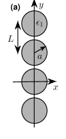
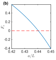
Figure 1: (a): A periodic array of circular cylinders surrounded by air. (b) $F_{e}$ of the first ASW as a function of radius $a$ for $\epsilon_{1}=8.2$.

we consider a single periodic array of dielectric circular cylinders surrounded by air. The radius and dielectric constant of the cylinders are $a$ and $\epsilon_{1}$, respectively. BICs on such a periodic array have been extensively investigated before shipman03 ; hu15 ; bulg14b ; yuan17 . For $a=0.4L$, $\epsilon_{1}=8.2$ and the $E$ polarization, the array supports five ASWs and one propagating BIC. The frequencies and Bloch wavenumbers of these BICs are listed in the first and second columns of Table 1, respectively.

$\omega_{*}L/(2\pi c)$	$\beta_{*}L/(2\pi)$	$a_{2}$: Eq. (36)	$a_{2}$: approximation
$0.4104$	$0$	$0.0325$	$0.0325$
$0.5458$	$0$	$0.1330$	$0.1331$
$0.7087$	$0$	$0.1429$	$0.1428$
$0.8080$	$0$	$0.0824$	$0.0825$
$0.8749$	$0$	$0.0766$	$0.0769$
$0.6872$	$0.2038$	$0.1033$	$0.1040$

Table 1: Frequencies and Bloch wavenumbers of six BICs on a periodic array of circular cylinders with radius $a=0.4L$ and dielectric constant $\epsilon_{1}=8.2$, and their exact and approximate coefficients $a_{2}$.

First, we check the formula for $\mbox{Im}(\omega)$ for ordinary BICs where $\phi_{1}$ radiates power to infinity. The periodic array has reflection symmetries in both $x$ and $y$ directions, thus, Eq. (33) is applicable. In terms of the normalized frequency and normalized wavenumber, Eq. (33) can be written as

$$\frac{\mbox{Im}(\omega)L}{2\pi c}\sim-a_{2}\left[\frac{(\beta-\beta_{*})L}{2\pi}\right]^{2},$$ (35)

where $a_{2}$ is a dimensionless coefficient given by

$$a_{2}=\frac{\pi\left(|F_{e}|^{2}+|F_{o}|^{2}\right)}{2L^{2}k_{*}\alpha_{*}\int\epsilon|\phi_{*}|^{2}d{\bm{r}}}.$$ (36)

Recall that $F_{e}$ and $F_{o}$ are real, and one of them is always zero. For each BIC listed in Table 1, we calculate $a_{2}$ by Eq. (36), and also find an approximation of $a_{2}$ by a quadratic polynomial fitting the numerical values of $\mbox{Im}(\omega)$ for $\beta=\beta_{*}$ and $\beta_{*}\pm 0.02\pi/L$. As shown in the third and fourth columns of Table 1, the exact and approximate values of $a_{2}$ agree very well. This confirms that Eqs. (35) and (36) are correct.

We are interested in the special BICs surrounded by strong resonances with $Q\sim 1/(\beta-\beta_{*})^{4}$. It is known that the symmetric standing waves (even in $y$) are examples of such special BICs yuan17_2 , and they exist when $a$ and $\epsilon_{1}$ lie on a curve in the $a\epsilon_{1}$ plane yuan17 . Bulgakov and Maksimov bulg17_2 found a number of ASWs which also have this special property. Using the perturbation theory developed in previous sections, we can find these special BICs systematically by searching the parameters $a$ and $\epsilon_{1}$, such that $F_{e}=0$ for an $x$-even BIC or $F_{o}=0$ for an $x$-odd BIC. The first ASW listed in Table 1, with $\omega_{*}L/(2\pi c)=0.4101$ for $a=0.4L$ and $\epsilon_{1}=8.2$, is even in $x$. We calculate $F_{e}$ for this BIC as a function of $a$ with a fixed $\epsilon_{1}=8.2$. The result is shown in Fig. 1(b). Since $F_{e}$ is real and changes signs, it must have a zero. It turns out that $F_{e}=0$ for $a=0.4404L$. The frequency of the corresponding ASW is $\omega_{*}L/(2\pi c)=0.3950$. Its wave field pattern is shown in Fig. 2(a).

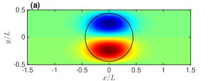
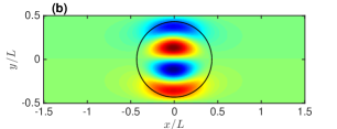
Figure 2: Wave field patterns of two special $x$-even ASWs on periodic arrays of circular cylinders with $\epsilon_{1}=8.2$. (a) The first ASW for $a=0.4404L$. (b) The fifth ASW for $a=0.4323L$.

For other values of $\epsilon_{1}>1$, $F_{e}$ of the first ASW can still reach zero for a properly chosen $a$. Those values of $a$ and $\epsilon_{1}$ such that $F_{e}=0$ for the first ASW give rise to a curve in the $a\epsilon_{1}$ plane, shown as the red solid line in Fig. 3(a).

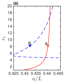
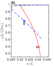
Figure 3: (a): Parameters of the periodic array for two special ASWs: the first ASW (red solid curve) and the fifth ASW (blue dashed curve). (b) The corresponding frequencies of the two special ASWs. Points ${\sf A}$ and ${\sf B}$ correspond to Figs. 2(a) and 2(b), respectively.

The corresponding frequency $\omega_{*}$ is shown with $a$ as the solid red curve in Fig. 3(b). It appears that as $\epsilon_{1}$ is increased, the related $a$ increases and approaches a constant as infinity. It should be pointed that the first ASW exists for all $\epsilon_{1}>1$ and $0<a\leq 0.5L$ hu15 . The curve represents those parameter values such that the ASW becomes a special BIC surrounded by strong resonances.

For the other BICs listed in Table 1, we also attempt to find parameters $a$ and $\epsilon_{1}$ such that $F_{e}=F_{o}=0$. It seems that only the fifth ASW, with $\omega_{*}L/(2\pi c)=0.8749$ for $a=0.4L$ and $\epsilon_{1}=8.2$, can be tuned to a special BIC. For $\epsilon_{1}=8.2$, the fifth ASW, which is also even in $x$, gives $F_{e}=0$ for $a=0.4323L$. Its frequency is $\omega_{*}L/(2\pi c)=0.7701$, and its field pattern is shown in Fig. 2(b). For other values of $\epsilon_{1}$, we also found the corresponding values of $a$ such that $F_{e}=0$ for the fifth ASW. The results are given as a curve in the $a\epsilon_{1}$ plane, i.e., the blue dashed line in Fig. 3(a). The corresponding frequency $\omega_{*}$ is shown as the blue dashed line in Fig. 3(b). Notice that $\epsilon_{1}$ has a lower bound around $4.67$, and it is achieved as $a\to 0.5L$. In addition, $a$ as a function of $\epsilon_{1}$, has a minimum around $\epsilon_{1}=5.35$, and it seems to approach a constant as $\epsilon_{1}$ tends to infinity.

In order to evaluate $F_{e}$ for an $x$-even BIC, we need to calculate the $x$-even diffraction solution $u_{e}=C(u_{l}+u_{r})$, where $C$ is chosen so that $u_{e}$ is ${\cal PT}$-symmetric and $C=e^{-i\tau}$ for a real constant $\tau$. As shown in yuan17_4 , this leads to

$$\varphi_{e}\sim 2\cos(\alpha_{*}x\pm\tau),\quad x\to\pm\infty.$$ (37)

In Fig. 4,

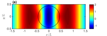
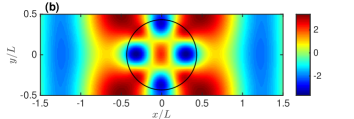
Figure 4: (a) and (b): Diffraction solutions $\varphi_{e}$ corresponding to the special ASWs shown in Figs. 2(a) and 2(b), respectively.

we show the diffraction solutions corresponding to the two special ASWs shown in Fig. 2.

In Sec. III, we argued that if $\mbox{Im}(\omega_{2})=0$, then $\mbox{Im}(\omega_{3})$ should also be zero, and $\mbox{Im}(\omega)$ should be proportional to $(\beta-\beta_{*})^{4}$ in general. For the two ASWs shown in Fig. 2, we check this result by computing the complex frequencies of some nearby resonant modes directly. In Fig. 5,

Figure 5: Imaginary parts of the complex frequencies vs. $\beta$ for resonant modes near ASWs shown in Fig. 2(a) ($\circ$) and Fig. 2(b) ($\ast$), respectively.

we show $\mbox{Im}(\omega)$ as functions of $\beta$ in a logarithmic scale for some resonant modes near these two ASWs. The numerical results confirm the fourth order relation between $\mbox{Im}(\omega)$ and $\beta$.

VI Conclusion

BICs on periodic structures are surrounded by resonant modes with $Q$-factors approaching infinity. High-$Q$ resonances and the resulting strong local field enhancement have important applications in lasing, nonlinear optics, etc. On 2D periodic structures, the $Q$-factors of the resonant modes near a BIC usually satisfy $Q\sim 1/(\beta-\beta_{*})^{2}$, where $\beta$ and $\beta_{*}$ are the Bloch wavenumbers of the resonant mode and the BIC, respectively. In this paper, we derived a general condition for special BICs so that their nearby resonant modes have $Q\sim 1/(\beta-\beta_{*})^{4}$. These special BICs produce high-$Q$ resonances for a very large range of $\beta$, and they are useful because precise control of $\beta$ may be difficult in practice. The conditions for the special BICs are given in integrals involving the BIC and related diffraction solutions, and they imply that the first order perturbation $\phi_{1}$ does not radiate power to infinity. Numerical examples are given for two families of ASWs on a periodic array of circular cylinders.

In practical applications, the BICs always dissolve into resonant modes with finite $Q$-factors, because the structures are always finite and fabrication errors will break the required symmetries and periodicity. We expect the special BICs have advantages over the ordinary BICs in practical structures with fabrication errors and in finite structures, but a rigorous analysis is still under development. In addition, the results of this paper are restricted to 2D structures. Clearly, it is worthwhile to derive similar conditions for special BICs on bi-periodic three-dimensional (3D) structures and rotationally symmetric 3D structures.

Appendix

For operator ${\cal L}$ given in Eq. (13), it is easy to verify that

$$\overline{\phi}_{*}{\cal L}\phi_{1}-\phi_{1}\overline{\cal L}\overline{\phi}_{*}=\nabla\cdot\left(\overline{\phi}_{*}\nabla\phi_{1}-\phi_{1}\nabla\overline{\phi}_{*}\right)+2i\beta_{*}\partial_{y}(\phi_{1}\overline{\phi}_{*}),$$

where $\nabla$ is the 2D gradient operator. The integral on $\Omega$ of the right hand side can be reduced to an integral on $\partial\Omega$ (the boundary of $\Omega$) by the divergence theorem. It is zero, since $\phi_{*}$ and $\phi_{1}$ are periodic in $y$ and $\phi_{*}\to 0$ exponentially as $|x|\to\infty$. Meanwhile, $\phi_{*}$ satisfies Eq. (10), thus $\int_{\Omega}\overline{\phi}_{*}{\cal L}\phi_{1}d{\bm{r}}=0$. From Eq. (11) for $\phi_{1}$, it is clear that

$$\int_{\Omega}\overline{\phi}_{*}\left[-2i\partial_{y}\phi_{*}+2(\beta_{*}-k_{*}k_{1}\epsilon)\phi_{*}\right]d{\bm{r}}=0.$$

This leads to Eq. (14). Meanwhile, $\int\overline{\phi}_{*}\partial_{y}\phi_{*}d{\bm{r}}$ is pure imaginary, since

$$\int_{\Omega}\overline{\phi}_{*}\partial_{y}\phi_{*}d{\bm{r}} = \int_{\Omega}\partial_{y}|\phi_{*}|^{2}d{\bm{r}}-\int_{\Omega}\phi_{*}\partial_{y}\overline{\phi}_{*}d{\bm{r}}$$

$$= -\int_{\Omega}\phi_{*}\partial_{y}\overline{\phi}_{*}d{\bm{r}}.$$

Therefore, $k_{1}$ is real.

Similarly, we have $\int_{\Omega}\overline{\phi}_{*}{\cal L}\phi_{2}d{\bm{r}}=0$. Multiplying both sides of Eq. (12) and integrating on $\Omega$, we obtain

$$k_{2}=\frac{\int_{\Omega}(1-k_{1}^{2}\epsilon)|\phi_{*}|^{2}d{\bm{r}}+\int_{\Omega}R\,d{\bm{r}}}{2k_{*}\int_{\Omega}\epsilon|\phi_{*}|^{2}d{\bm{r}}},$$

where $R=\overline{\phi}_{*}[-2i\partial_{y}\phi_{1}+2(\beta_{*}-k_{*}k_{1}\epsilon)\phi_{1}]$. Therefore,

$$\mbox{Im}(k_{2})=\frac{\mbox{Im}\left[\int_{\Omega}R\,d{\bm{r}}\right]}{2k_{*}\int_{\Omega}\epsilon|\phi_{*}|^{2}d{\bm{r}}}.$$

From the complex conjugate of Eq. (11), we obtain

$$\int_{\Omega_{h}}\phi_{1}\overline{\cal L}\overline{\phi}_{1}d{\bm{r}}=\int_{\Omega_{h}}R\,d{\bm{r}},$$

where $\Omega_{h}$ is the rectangular domain defined in Sec. IV. The right hand side above requires an integration by parts that switches the integral from $\phi_{1}\partial_{y}\overline{\phi}_{*}$ to $-\overline{\phi}_{*}\partial_{y}\phi_{1}$. Meanwhile, it is easy to verify that

$$\int_{\Omega_{h}}\phi_{1}\overline{\cal L}\overline{\phi}_{1}d{\bm{r}}=\int_{\partial\Omega_{h}}\phi_{1}\frac{\partial\overline{\phi}_{1}}{\partial\nu}ds$$

$$+\int_{\Omega_{h}}\left[(k_{*}^{2}\epsilon-\beta_{*}^{2})|\phi_{1}|^{2}-|\nabla\phi_{1}|^{2}-2i\beta_{*}\phi_{1}\frac{\partial\overline{\phi}_{1}}{\partial y}\right]d{\bm{r}},$$

where $\partial\Omega_{h}$ is the boundary of $\Omega_{h}$ and $\nu$ is its unit outward normal vector. The second term in the right hand side above is real. Therefore,

$$\mbox{Im}\left[\int_{\Omega_{h}}R\,d{\bm{r}}\right]=\mbox{Im}\left[\int_{\partial\Omega_{h}}\phi_{1}\frac{\partial\overline{\phi}_{1}}{\partial\nu}ds\right].$$

Since $\phi_{1}$ is periodic in $y$, the line integrals at $y=\pm L/2$ are canceled. Therefore

$$\int_{\partial\Omega_{h}}\phi_{1}\frac{\partial\overline{\phi}_{1}}{\partial\nu}ds=\int_{-L/2}^{L/2}\left[\phi_{1}\frac{\partial\overline{\phi}_{1}}{\partial x}\right]^{x=h}_{x=-h}dy,$$

where $P(x,y)|_{x=-h}^{x=h}$ denotes $P(h,y)-P(-h,y)$.

For $|x|>D$, the equation for $\phi_{1}$ is quite simple. It is not difficult to see that

$$\phi_{1}=d_{0}^{\pm}e^{\pm i\alpha_{*}x}+\sum_{j\neq 0}d_{j}^{\pm}(x)e^{i2\pi jy/L}e^{\pm\gamma_{*j}x}$$

for $x>D$ and $x<-D$ respectively, where $\gamma_{*j}=-i\alpha_{*j}$ is positive, $d_{0}^{\pm}$ are unknown coefficients, and $d_{j}^{\pm}(x)$ ($j\neq 0$) are unknown linear polynomials of $x$. The above gives

$$\lim_{h\to+\infty}\int_{-L/2}^{L/2}\left[\phi_{1}\frac{\partial\overline{\phi}_{1}}{\partial x}\right]^{x=h}_{x=-h}dy=-iL\alpha_{*}(|d_{0}^{+}|^{2}+|d_{0}^{-}|^{2}),$$

and $\mbox{Im}\left[\int_{\Omega}R\,d{\bm{r}}\right]=-L\alpha_{*}(|d_{0}^{+}|^{2}+|d_{0}^{-}|^{2})$, and finally Eq. (16).

To show Eq. (24), we notice that

$$\overline{\varphi}_{l}{\cal L}\phi_{1}-\phi_{1}\overline{\cal L}\overline{\varphi}_{l}=\nabla\cdot[\overline{\varphi}_{l}\nabla\phi_{1}-\phi_{1}\nabla\overline{\varphi}_{l}]+2i\beta_{*}\partial_{y}(\phi_{1}\overline{\varphi}_{l}).$$

Since $\varphi_{l}$ satisfies the Helmholtz equation and both $\phi_{1}$ and $\varphi_{l}$ are periodic in $y$, we have

$$\int_{\Omega_{h}}\overline{\varphi}_{l}{\cal L}\phi_{1}d{\bm{r}}=\int_{\partial\Omega_{h}}\left[\overline{\varphi}_{l}\frac{\partial\phi_{1}}{\partial\nu}-\phi_{1}\frac{\partial\overline{\varphi}_{l}}{\partial\nu}\right]ds.$$

In the right hand side above, the integrals on the two edges at $y=\pm L/2$ are canceled. Therefore

$$\int_{\Omega_{h}}\overline{\varphi}_{l}{\cal L}\phi_{1}d{\bm{r}}=\int_{-L/2}^{L/2}\left[\overline{\varphi}_{l}\frac{\partial\phi_{1}}{\partial x}-\phi_{1}\frac{\partial\overline{\varphi}_{l}}{\partial x}\right]^{x=h}_{x=-h}dy.$$

Based on the asymptotic formula (20), it is easy to show that as $h\to+\infty$, the right hand side above tend to $2iL\alpha_{*}(d_{0}^{+}\overline{T}_{l}+d_{0}^{-}\overline{R}_{l})$. This leads to Eq. (24). The proof for Eq. (25) is similar.

References

- (1) J. von Neumann and E. Wigner, “Über merkwürdige diskrete eigenwerte,” Z. Physik 50, 291-293 (1929).
- (2) C. W. Hsu, B. Zhen, A. D. Stone, J. D. Joannopoulos, and M. Soljačić, “Bound states in the continuum,” Nat. Rev. Mater. 1, 16048 (2016).
- (3) D. V. Evans and C. M. Linton, “Trapped modes in open channels,” J. Fluid Mech. 225, 153-175 (1991).
- (4) J. Goldstone and R. L. Jaffe, “Bound states in twisting tubes,” Phys. Rev. B 45, 14100-14107 (1992).
- (5) D. V. Evans, M. Levitin and D. Vassiliev, “Existence theorems for trapped modes,” J. Fluid Mech. 261, 21-31 (1994).
- (6) D. V. Evans and R. Porter, “Trapped modes embedded in the continuous spectrum,” Q. J. Mech. Appl. Math. 51(2), 263-274 (1998).
- (7) E. N. Bulgakov and A. F. Sadreev, “Bound states in the continuum in photonic waveguides inspired by defects,” Phys. Rev. B 78, 075105 (2008).
- (8) Y. Plotnik, O. Peleg, F. Dreisow, M. Heinrich, S. Nolte, A. Szameit, and M. Segev, “Experimental observation of optical bound states in the continuum,” Phys. Rev. Lett. 107, 183901 (2011).
- (9) M. I. Molina, A. E. Miroshnichenko, and Y. S. Kivshar, “Surface bound states in the continuum,” Phys. Rev. Lett. 108, 070401 (2012).
- (10) S. Weimann, Y. Xu, R. Keil, A. E. Miroshnichenko, A. Tünnermann, S. Nolte, A. A. Sukhorukov, A. Szameit, and Y. S. Kivshar, “Compact surface Fano states embedded in the continuum of the waveguide arrays,” Phys. Rev. Lett. 111, 240403 (2013).
- (11) C. L. Zou, J.-M. Cui, F.-W. Sun, X. Xiong, X.-B. Zou, Z.-F. Han, and G.-C. Guo, “Guiding light through optical bound states in the continuum for ultrahigh-Q microresonantors,” Laser & Photonics Rev. 9, 114-119 (2015).
- (12) A.-S. Bonnet-Bendhia and F. Starling, “Guided waves by electromagnetic gratings and nonuniqueness examples for the diffraction problem,” Math. Methods Appl. Sci. 17, 305-338 (1994).
- (13) P. Paddon and J. F. Young, “Two-dimensional vector-coupled-mode theory for textured planar waveguides,” Phys. Rev. B 61, 2090-2101 (2000).
- (14) S. G. Tikhodeev, A. L. Yablonskii, E. A Muljarov, N. A. Gippius, and T. Ishihara, “Quasi-guided modes and optical properties of photonic crystal slabs,” Phys. Rev. B 66, 045102 (2002).
- (15) S. P. Shipman and S. Venakides, “Resonance and bound states in photonic crystal slabs,” SIAM J. Appl. Math. 64, 322-342 (2003).
- (16) S. Shipman and D. Volkov, “Guided modes in periodic slabs: existence and nonexistence,” SIAM J. Appl. Math. 67, 687–713 (2007).
- (17) J. Lee, B. Zhen, S. L. Chua, W. Qiu, J. D. Joannopoulos, M. Soljačić, and O. Shapira, “Observation and differentiation of unique high-Q optical resonances near zero wave vector in macroscopic photonic crystal slabs,” Phys. Rev. Lett. 109, 067401 (2012).
- (18) Z. Hu and Y. Y. Lu, “Standing waves on two-dimensional periodic dielectric waveguides,” Journal of Optics 17, 065601 (2015).
- (19) R. Porter and D. Evans, “Embedded Rayleigh-Bloch surface waves along periodic rectangular arrays,” Wave Motion 43, 29-50 (2005).
- (20) D. C. Marinica, A. G. Borisov, and S. V. Shabanov, “Bound states in the continuum in photonics,” Phys. Rev. Lett. 100, 183902 (2008).
- (21) R. F. Ngangali and S. V. Shabanov, “Electromagnetic bound states in the radiation continuum for periodic double arrays of subwavelength dielectric cylinders,” J. Math. Phys. 51, 102901 (2010).
- (22) C. W. Hsu, B. Zhen, S.-L. Chua, S. G. Johnson, J. D. Joannopoulos, and M. Soljačić, “Bloch surface eigenstates within the radiation continuum,” Light Sci. Appl. 2, e84 (2013).
- (23) C. W. Hsu, B. Zhen, J. Lee, S.-L. Chua, S. G. Johnson, J. D. Joannopoulos, and M. Soljačić, “Observation of trapped light within the radiation continuum,” Nature 499, 188–191 (2013).
- (24) Y. Yang, C. Peng, Y. Liang, Z. Li, and S. Noda, “Analytical perspective for bound states in the continuum in photonic crystal slabs,” Phys. Rev. Lett. 113, 037401 (2014).
- (25) B. Zhen, C. W. Hsu, L. Lu, A. D. Stone, and M. Soljačič, “Topological nature of optical bound states in the continuum,” Phys. Rev. Lett. 113, 257401 (2014).
- (26) E. N. Bulgakov and A. F. Sadreev, “Bloch bound states in the radiation continuum in a periodic array of dielectric rods,” Phys. Rev. A 90, 053801 (2014).
- (27) E. N. Bulgakov and A. F. Sadreev, “Light trapping above the light cone in one-dimensional array of dielectric spheres,” Phys. Rev. A 92, 023816 (2015).
- (28) E. N. Bulgakov and D. N. Maksimov, “Light guiding above the light line in arrays of dielectric nanospheres,” Opt. Lett. 41, 3888 (2016).
- (29) R. Gansch, S. Kalchmair, P. Genevet, T. Zederbauer, H. Detz, A. M. Andrews, W. Schrenk, F. Capasso, M. Lončar, and G. Strasser, “Measurement of bound states in the continuum by a detector embedded in a photonic crystal,” Light: Science & Applications 5, e16147 (2016).
- (30) L. Li and H. Yin, “Bound States in the Continuum in double layer structures,” Sci. Rep. 6 26988 (2016).
- (31) X. Gao, C. W. Hsu, B. Zhen, X. Lin, J. D. Joannopoulos, M. Soljačić, and H. Chen, “Formation mechanism of guided resonances and bound states in the continuum in photonic crystal slabs,” Sci. Rep. 6, 31908 (2016).
- (32) L. Ni, Z. Wang, C. Peng, and Z. Li, “Tunable optical bound states in the continuum beyond in-plane symmetry protection,” Phys. Rev. B 94, 245148 (2016).
- (33) L. Yuan and Y. Y. Lu, “Propagating Bloch modes above the lightline on a periodic array of cylinders,” J. Phys. B: Atomic, Mol. and Opt. Phys. 50, 05LT01 (2017).
- (34) E. N. Bulgakov and A. F. Sadreev, “Bound states in the continuum with high orbital angular momentum in a dielectric rod with periodically modulated permittivity,” Phys. Rev. A96, 013841 (2017).
- (35) Z. Hu and Y. Y. Lu, “Propagating bound states in the continuum at the surface of a photonic crystal,” J. Opt. Soc. Am. B 34, 1878-1883 (2017).
- (36) E. N. Bulgakov and D. N. Maksimov, “Topological bound states in the continuum in arrays of dielectric spheres,” Phys. Rev. Lett. 118, 267401 (2017).
- (37) L. Yuan and Y. Y. Lu, “Bound states in the continuum on periodic structures: perturbation theory and robustness,” Opt. Lett. 42(21) 4490-4493 (2017).
- (38) E. N. Bulgakov and D. N. Maksimov, “Bound states in the continuum and polarization singularities in periodic arrays of dielectric rods,” Phys. Rev. A 96, 063833 (2017).
- (39) Z. Hu and Y. Y. Lu, “Resonances and bound states in the continuum on periodic arrays of slightly noncircular cylinders,” J. Phys. B: At. Mol. Opt. Phys. 51, 035402 (2018).
- (40) S. P. Shipman and S. Venakides, “Resonant transmission near nonrobust periodic slab modes,” Phys. Rev. E 71, 026611 (2005).
- (41) S. Shipman and H. Tu, “Total resonant transmission and reflection by periodic structures,” SIAM J. Appl. Math. 72, 216-239 (2012).
- (42) V. Mocella and S. Romano, “Giant field enhancement in photonic lattices,” Phys. Rev. B 92, 155117 (2015).
- (43) J. W. Yoon, S. H. Song, and R. Magnusson, “Critical field enhancement of asymptotic optical bound states in the continuum,” Sci. Rep. 5, 18301 (2015).
- (44) A. Kodigala, T. Lepetit, Q. Gu, B. Bahari, Y. Fainman, and B. Kanté, “Lasing action from photonic bound states in continuum,” Nature 541, 196-199 (2017).
- (45) L. Yuan and Y. Y. Lu, “Strong resonances on periodic arrays of cylinders and optical bistability with weak incident waves,” Phys. Rev. A 95, 023834 (2017)
- (46) J. M. Foley, S. M. Young, and J. D. Phillips, “Symmetry-protected mode coupling near normal incidence for narrow-band transmission filtering in a dielectric grating,” Phys. Rev. B 89, 165111 (2014).
- (47) X. Cui, H. Tian, Y. Du, G. Shi, and Z. Zhou, “Normal incidence filter using symmetry-protected modes in dielectric subwavelength gratings,” Sci. Rep. 6, 36066 (2016)
- (48) Z. F. Sadrieva, I. S. Sinev, K. L. Koshelev, A. Samusev, I. V. Iorsh, O. Takayama, R. Malureanu, A. A. Bogdanov, and A. V. Lavrinenko, “Transition from optical bound states in the continuum to leaky resonances: Role of substrate and roughness,” ACS Photonics 4, 723-727 (2017).
- (49) E. N. Bulgakov and D. N. Maksimov, “Light enhancement by quasi-bound states in the continuum in dielectric arrays,” Opt. Express 25(13), 14134-14147 (2017)
- (50) A. Taghizadeh and I.-S. Chung, “Quasi bound states in the continuum with few unit cells for photonic crystal slab,” Appl. Phys. Lett. 111, 031114 (2017).
- (51) E. N. Bulgakov and A. F. Sadreev, “Near-bound states in the radiation continuum in circular array of dielectric rods,” arXiv:1711.05965.