A semiclassical theory of phase-space dynamics of interacting bosons

Abstract

We study the phase-space representation of dynamics of bosons in the semiclassical regime where the occupation number of the modes is large. To this end, we employ the van Vleck-Gutzwiller propagator to obtain an approximation for the Green’s function of the Wigner distribution. The semiclassical analysis incorporates interference of classical paths and reduces to the truncated Wigner approximation (TWA) when the interference is ignored. Furthermore, we identify the Ehrenfest time after which the TWA fails. As a case study, we consider a single-mode quantum nonlinear oscillator, which displays collapse and revival of observables. We analytically show that the interference of classical paths leads to revivals, an effect that is not reproduced by the TWA or a perturbative analysis.

I Introduction

The crucial difference between quantum mechanics and a statistical theory based on classical mechanics is the method of computing the transition probability between an initial and a final state Feynman et al. (1963). In the classical theory, the transition probability is the sum over probabilities of the paths connecting the two states. In contrast, in quantum mechanics, the transition probability is obtained by first summing the amplitudes of all the connecting paths and then squaring the sum. This procedure leads to interference, a feature absent in the classical theory. An archetypal example of interference is a double-slit experiment in which a beam of particles after passing through two slits forms an oscillating intensity pattern on a screen Feynman et al. (1963).

The aforementioned difference between the theories can be systematically studied in the semiclassical regime (where the typical action $\gg\hbar$, the reduced Planck’s constant). In this regime, a probability amplitude can be approximated by the contributions from a subset of all connecting paths: the classical paths Schulman (2005); Morette (1951). (This is the case with the textbook treatment of the double-slit experiment.) Crucially, within this semiclassical approximation, the transition probability retains interference of paths, albeit classical ones. The role of classical trajectories in quantum dynamics was first elucidated by van Vleck Vleck (1928). Later, Gutzwiller extended the van Vleck propagator by including Maslov indices and used it to derive his trace formula Gutzwiller (1971). The role of classical paths in quantum mechanics has been extensively studied; for example, in scattering Pechukas (1969), localization Rammer (2004); Brouwer and Altland (2008), quantum kicked rotor Tian et al. (2005), level statistics Aleiner and Larkin (1997); Müller et al. (2005), quantum work Jarzynski et al. (2015), the Helium atom Wintgen et al. (1992) and quantum transport Richter and Richter (2000); Baranger et al. (1993).

In this paper, we study a semiclassical approximation of the phase-space dynamics of interacting bosons in the Wigner-Weyl representation. In this representation, unitary evolution of an initial quantum state in the Hilbert space is equivalent to evolution of an initial Wigner distribution in phase space in accordance to the Moyal’s equation Groenewold (1946); Moyal (1949); Curtright et al. (2014). The reduction of the state space from a high-dimensional Hilbert space to a lower-dimensional phase space makes the phase-space picture particularly useful for implementing approximations of quantum dynamics. An approximation that is usually made is a mean-field approach. In this case, the distribution is approximated at all times by a delta function whose location is determined by the classical Hamilton’s equations. The Gross-Pitaevskii equation and its discrete versions fall under this category.

An improvement over the mean-field description is the truncated Wigner approximation (TWA) Heller (1991); Steel et al. (1998); Blakie et al. (2008), where the initial distribution is extended and is the Wigner transform of a quantum state. The subsequent dynamics of the Wigner distribution is still classical. Equivalently, the Moyal’s equation is replaced by the classical Liouville’s equation. In the literature, the TWA is sometimes called a semiclassical method eventhough it lacks interference effects. Quantum corrections to the TWA for interacting bosons were studied by A. Polkovnikov Polkovnikov (2003, 2010) using a perturbation theory with the TWA as its zeroth-order approximation. In particular, a nonlinear oscillator was studied whose quantum dynamics exhibits collapse and revival of coherences. The perturbative analysis describes the initial collapse, with increasing accuracy with the order of the perturbation parameter. It fails to describe revivals in the system because the analysis still lacks interference of classical paths.

We study semiclassical dynamics of a general Bose system in phase space that incorporates interference of classical paths and makes comparison with the TWA transparent. In particular, our analysis identifies the Ehrenfest time associated with the TWA as the time when interference of classical paths becomes important. As a case study, we investigate the nonlinear oscillator and show that the semiclassical dynamics leads to revivals. Recently, others have also applied semiclassical methods to bosons. For example, these methods have been applied to coherent backscattering Engl et al. (2014) and autocorrelation functions Tomsovic et al. (2017) in the Bose-Hubbard model. In addition, the semiclassical Herman-Kluck propagator has been used to study boson dynamics Simon and Strunz (2014); Ray et al. (2016).

The remainder of the paper is organized as follows. First, we define the phase space of a bosonic system and the Green’s function of a Wigner distribution in Sec. II and Sec. III, respectively. A semiclassical approximation of this Green’s function is obtained in Sec. IV. In Sec. IV.1, we find that our semiclassical formalism reduces to the TWA when the interference terms are ignored. Next, we discuss Ehrenfest times associated with the TWA and semiclassical approximation in Sec. IV.2. Subsequently, we apply our formalism to analytically study of a nonlinear oscillator in Sec. V and conclude in Sec. VI.

II Phase-space formulation of a bosonic system

A bosonic system with a finite number of modes can be described in terms of annihilation and creation operators $\hat{a}_{j}$ and $\hat{a}^{\dagger}_{j}$, respectively, with $j=1,\dots,d$, where $d$ is the number of modes. For example, the modes could be the sites of a Bose-Hubbard model or spin components of a single-mode Bose-Einstein condensate. The operators satisfy the commutation relations $[a_{j},a^{\dagger}_{k}]=\delta_{jk}$, where $\delta_{jk}$ is the Kronecker delta function. To construct the phase space, we first define the quadrature operators $\hat{x}_{j}=\sqrt{\hbar/2}\,(\hat{a}_{j}+\hat{a}^{\dagger}_{j})$ and $\hat{p}_{j}=-i\sqrt{\hbar/2}\,(\hat{a}_{j}-\hat{a}^{\dagger}_{j})$ satisfying the canonical commutation relations $[\hat{x}_{j},\hat{p}_{k}]=i\hbar\delta_{jk}$. The eigenstates of $\hat{x}_{j}$ satisfy $\hat{x}_{j}\left|\mathbf{x}\right\rangle=x_{j}\left|\mathbf{x}\right\rangle$ for all $j\in\{1,\cdots,d\}$, with “position” $\mathbf{x}=(x_{1},x_{2},\dots,x_{d})$. Similarly, the eigenstates of $\hat{p}_{j}$ satisfy $\hat{p}_{j}\left|\mathbf{p}\right\rangle=p_{j}\left|\mathbf{p}\right\rangle$, with “momentum” $\mathbf{p}=(p_{1},p_{2},\dots,p_{d})$. The eigenstates form a complete basis with $\left\langle\mathbf{x}^{\prime}|\mathbf{x}\right\rangle=\delta(\mathbf{x}-\mathbf{x}^{\prime})$, $\left\langle\mathbf{p}^{\prime}|\mathbf{p}\right\rangle=\delta(\mathbf{p}-\mathbf{p}^{\prime})$ and $\int d\mathbf{x}\,\left|\mathbf{x}\right\rangle\left\langle\mathbf{x}\right|=\int d\mathbf{p}\,\left|\mathbf{p}\right\rangle\left\langle\mathbf{p}\right|=1$, where $\delta(\mathbf{z})$ is a Dirac delta function and the integrals are over $\mathbb{R}^{d}$. We construct a phase space by imposing $\{x_{i},p_{j}\}=\delta_{ij}$, where $\{.,.\}$ is the Poisson bracket. We will refer to $\mathbf{r}=(\mathbf{x},\mathbf{p})$ as a phase-space point. Thus, by introducing quadrature operators, we have mapped the kinematics of a many-body boson system with $d$ modes to that of a single particle in $d$-dimensional position or configuration space.

The Wigner transform Curtright et al. (2014); Hillery et al. (1984) maps an operator $\hat{\mathcal{O}}$, a function of $\hat{a}_{j}$ and $\hat{a}^{\dagger}_{j}$ or $\hat{x}_{j}$ and $\hat{p}_{j}$, to its Weyl symbol $\mathcal{O}$ in the phase space. In fact,

$$\mathcal{O}(\mathbf{r})=\int d\mathbf{q}\,\left\langle\mathbf{x}+\tfrac{1}{2}\mathbf{q}|\hat{\mathcal{O}}|\mathbf{x}-\tfrac{1}{2}\mathbf{q}\right\rangle e^{-i\mathbf{p}\cdot\mathbf{q}/\hbar},$$ (1)

where $\mathbf{r}=(\mathbf{x},\mathbf{p})$, ${\mathbf{p}\cdot\mathbf{q}}$ is the dot product between $\mathbf{p}$ and $\mathbf{q}$, and the integral is over the configuration space $\mathbf{q}\in\mathbb{R}^{d}$. In particular, the Wigner distribution $W(\mathbf{r},t)$ at time $t$ is the Weyl symbol of the density operator $\hat{\rho}(t)$, up to a factor of $1/(2\pi\hbar)^{d}$, i.e.,

$$W(\mathbf{r},t)=\frac{1}{(2\pi\hbar)^{d}}\int d\mathbf{q}\,\left\langle\mathbf{x}+\tfrac{1}{2}\mathbf{q}|\hat{\rho}(t)|\mathbf{x}-\tfrac{1}{2}\mathbf{q}\right\rangle e^{-i\mathbf{p}\cdot\mathbf{q}/\hbar},$$ (2)

These definitions imply that $\int d\mathbf{r}\,W(\mathbf{r},t)=1$ and in the Schrödinger picture, the expectation value of an operator $\hat{\mathcal{O}}$ at a time $t$ is

$$\left\langle\hat{\mathcal{O}}(t)\right\rangle\equiv\operatorname{Tr}[\hat{\rho}(t)\hat{\mathcal{O}}]=\int d\mathbf{r}\,W(\mathbf{r},t)\mathcal{O}(\mathbf{r}),$$ (3)

where the integrals are over the phase space $\mathbb{R}^{2d}$. Equivalently, in the Heisenberg picture,

$$\left\langle\hat{\mathcal{O}}(t)\right\rangle\equiv\operatorname{Tr}[\hat{\rho}\,\hat{\mathcal{O}}(t)]=\int d\mathbf{r}\,W_{0}(\mathbf{r})\mathcal{O}(\mathbf{r},t),$$ (4)

where $W_{0}(\mathbf{r})$ is the initial Wigner distribution.

III Green’s function of the Wigner distribution

The Green’s function $G(\mathbf{r}_{f},\mathbf{r}_{i},t)$ of the Wigner distribution in the Schrödinger picture is defined by Moyal (1949); Berry et al. (1979); Marinov (1991); Dittrich et al. (2010)

$$W(\mathbf{r}_{f},t)=\int d\mathbf{r}_{i}\,G(\mathbf{r}_{f},\mathbf{r}_{i},t)W(\mathbf{r}_{i},0),$$ (5)

for $t\geq 0$ with $\mathbf{r}_{f}=(\mathbf{x}_{f},\mathbf{p}_{f})$, $\mathbf{r}_{i}=(\mathbf{x}_{i},\mathbf{p}_{i})$ and $G(\mathbf{r}_{f},\mathbf{r}_{i},0)=\delta(\mathbf{r}_{f}-\mathbf{r}_{i})$. In a seminal paper on quantum dynamics in phase space, Moyal called $G(\mathbf{r}_{f},\mathbf{r}_{i},t)$ the “temporal transformation function” Moyal (1949). He derived an expression for $G(\mathbf{r}_{f},\mathbf{r}_{i},t)$ in terms of Feynman propagators. We give a short and direct derivation.

The time evolution of the density operator is $\hat{\rho}(t)=\hat{U}(t)\hat{\rho}_{0}\hat{U}^{\dagger}(t)$, where $\hat{U}(t)$ and $\hat{\rho}_{0}$ are the unitary time-evolution and the initial density operator, respectively. We insert $\int d\mathbf{y}_{1}\left|\mathbf{y}_{1}\right\rangle\left\langle\mathbf{y}_{1}\right|=1$ and $\int d\mathbf{y}_{2}\left|\mathbf{y}_{2}\right\rangle\left\langle\mathbf{y}_{2}\right|=1$, with $\mathbf{y}_{1}$ and $\mathbf{y}_{2}$ in configuration space, into Eq. 2 and find

$$W(\mathbf{r}_{f},t) =\frac{1}{(2\pi\hbar)^{d}}\int d\mathbf{q}d\mathbf{y}_{1}d\mathbf{y}_{2}\,K\left(\mathbf{x}_{f}+\tfrac{1}{2}\mathbf{q}\,,\mathbf{y}_{1},t\right)$$ (6)

$$\quad\times\left\langle\mathbf{y}_{1}|\hat{\rho}_{0}|\mathbf{y}_{2}\right\rangle K^{*}\left(\mathbf{x}_{f}-\tfrac{1}{2}\mathbf{q},\mathbf{y}_{2},t\right)e^{-i\mathbf{p}_{f}\cdot\mathbf{q}/\hbar}\,,$$

where $K(\mathbf{x}_{f},\mathbf{x}_{i},t)=\left\langle\mathbf{x}_{f}\right|\hat{U}(t)\left|\mathbf{x}_{i}\right\rangle$ is the Feynman propagator in the configuration space. For notational simplicity, we have and will hereafter set $\hbar=1$. Next, we express the initial condition $\left\langle\mathbf{y}_{1}|\hat{\rho}_{0}|\mathbf{y}_{2}\right\rangle$ in terms of the initial Wigner distribution. To this end, we multiply Eq. 2, evaluated at $t=0$ and $\mathbf{r}=\mathbf{r}_{i}$, by $e^{i\mathbf{p}_{i}\cdot\mathbf{q}^{\prime}}$ and integrate over $\mathbf{p}_{i}$ to find

$$\int d\mathbf{p}_{i}\,e^{i\mathbf{p}_{i}\cdot\mathbf{q}^{\prime}/\hbar}W(\mathbf{r}_{i},0)=\left\langle\mathbf{x}_{i}+\tfrac{1}{2}\mathbf{q}^{\prime}|\hat{\rho}_{0}|\mathbf{x}_{i}-\tfrac{1}{2}\mathbf{q}^{\prime}\right\rangle$$ (7)

We substitute this expression in Eq. 6 and identify $\mathbf{y}_{1}=\mathbf{x}_{i}+\tfrac{1}{2}\mathbf{q}^{\prime}$ and $\mathbf{y}_{2}=\mathbf{x}_{i}-\tfrac{1}{2}\mathbf{q}^{\prime}$. From the definition of Green’s function in Eq. 5 we find

$$G(\mathbf{r}_{f},\mathbf{r}_{i},t)=\frac{1}{(2\pi\hbar)^{d}}\int d\mathbf{q}d\mathbf{q}^{\prime}\,K\left(\mathbf{x}_{f}+\tfrac{1}{2}\mathbf{q}\,,\mathbf{x}_{i}+\tfrac{1}{2}\mathbf{q}^{\prime}\,,t\right)\\ \times K^{*}\left(\mathbf{x}_{f}-\tfrac{1}{2}\mathbf{q}\,,\mathbf{x}_{i}-\tfrac{1}{2}\mathbf{q}^{\prime},t\right)e^{-i[\mathbf{p}_{f}\cdot\mathbf{q}-\mathbf{p}_{i}\cdot\mathbf{q}^{\prime}]/\hbar}.$$ (8)

Thus, the exact Green’s function of the Wigner distribution involves the product of two Feynman propagators in configuration space. We expect that this product will have interference terms.

IV Semiclassical approximation of the Green’s function

A quantum system is said to be in the semiclassical regime when the typical action (in units of $\hbar$) that appears in the path integral description of the Feynman propagator is much greater than one. For bosonic modes, this regime corresponds to large occupation numbers. In fact, the semiclassical approximation of the propagator, also known as the van Vleck-Gutzwiller propagator, is Littlejohn (1992); Schulman (2005)

$$K_{\rm SC}(\mathbf{x}_{f},\mathbf{x}_{i},t)=\sum_{b}\frac{e^{-i\mu^{b}\pi/2}}{(2\pi i\hbar)^{d/2}}\sqrt{\mathcal{D}^{b}(\mathbf{x}_{f},\mathbf{x}_{i},t)}e^{iS^{b}(\mathbf{x}_{f},\mathbf{x}_{i},t)/\hbar},$$ (9)

where the sum is over all classical paths, indexed by $b$, that start from position $\mathbf{x}_{i}$ and reach $\mathbf{x}_{f}$ in time $t$. The action $S^{b}(\mathbf{x}_{f},\mathbf{x}_{i},t)=\int_{0}^{t}d\tau\,L[\mathbf{x}_{\rm cl}^{b}(\tau),d\mathbf{x}_{\rm cl}^{b}(\tau)/d\tau]$, where $L$ is the system Lagrangian and $\mathbf{x}^{b}_{\rm cl}(\tau)$ is the position as a function of time $\tau$ of the $b$-th classical path with $\mathbf{x}^{b}_{\rm cl}(0)=\mathbf{x}_{i}$ and $\mathbf{x}^{b}_{\rm cl}(t)=\mathbf{x}_{f}$. Finally, $\mu^{b}$ is the Maslov index and $\mathcal{D}^{b}(\mathbf{x}_{f},\mathbf{x}_{i},t)=|\det\left[\partial^{2}S^{b}(\mathbf{x}_{f},\mathbf{x}_{i},t)/(\partial\mathbf{x}_{f}\partial\mathbf{x}_{i})\right]|$ is the absolute value of the determinant of a $d\times d$ matrix.

The number of classical paths contributing to $K_{\rm SC}(\mathbf{x}_{f},\mathbf{x}_{i},t)$ can be found by studying the dynamics of the initial Lagrangian manifold $\mathcal{M}_{i}$, the hyperplane $\mathbf{x}=\mathbf{x}_{i}$. Classical evolution of each point of $\mathcal{M}_{i}$ yields a final manifold $\mathcal{M}_{f}$. Figure 1 shows $\mathcal{M}_{i}$ and $\mathcal{M}_{f}$ for a two-dimensional example. The final manifold folds at singular positions $\mathbf{x}_{f}$ on $\mathcal{M}_{f}$ where the number of momenta $\mathbf{p}_{f}$ on $\mathcal{M}_{f}$ as a function of $\mathbf{x}_{f}$ changes. Parts of the manifold $\mathcal{M}_{f}$ between these singular regions are “branches”. The example in Fig. 1 has the three such branches. Crucially, the final momentum $\mathbf{p}_{f}(\mathbf{x}_{f},\mathbf{x}_{i},t)$, which, in general, is a multivalued function of $\mathbf{x}_{f}$ at fixed $\mathbf{x}_{i}$ and $t$, is unique on each branch. Therefore, classical paths connecting $\mathbf{x}_{i}$ and $\mathbf{x}_{f}$ can be indexed by the branches that intersect the manifold $\mathbf{x}=\mathbf{x}_{f}$. It is these branches which contribute to the van Vleck-Gutzwiller propagator in Eq. 9. For example, for the position $x_{f}$ shown in Fig. 1 has three paths that contribute to the propagator.

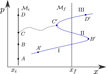
Figure 1: Classical dynamics of a manifold in a two-dimensional phase space $(x,p)$. An initial manifold $\mathcal{M}_{i}$, the line $x=x_{i}$ shown in black, evolves into the manifold $\mathcal{M}_{f}$, the curve shown in blue, at time $t$. For example, points $A$, $B$, $C$, and $D$ on $\mathcal{M}_{i}$ are mapped to $A^{\prime}$, $B^{\prime}$, $C^{\prime}$ and $D^{\prime}$ on $\mathcal{M}_{f}$, respectively. The classical path connecting $C$ and $C^{\prime}$ is also shown. The manifold $\mathcal{M}_{f}$ has three branches I, II and III separated by caustics $B^{\prime}$ and $C^{\prime}$. The line $x=x_{f}$ intersects $\mathcal{M}_{f}$ thrice; therefore, three paths start on $\mathcal{M}_{i}$ and reach position $x_{f}$ at time $t$.

Substitution of van Vleck-Gutzwiller propagator in Eq. 8 yields the semiclassical approximation to the Green’s function

$$G_{\rm SC}(\mathbf{r}_{f},\mathbf{r}_{i},t) =\frac{1}{(2\pi\hbar)^{2d}}\int d\mathbf{q}d\mathbf{q}^{\prime}\,e^{-i[\mathbf{p}_{f}\cdot\mathbf{q}-\mathbf{p}_{i}\cdot\mathbf{q}^{\prime}]/\hbar}\sum_{b}\sqrt{\mathcal{D}^{b}(\mathbf{x}_{f}+\mathbf{q}/2,\mathbf{x}_{i}+\mathbf{q}^{\prime}/2,t)}\,e^{iS^{b}(\mathbf{x}_{f}+\mathbf{q}/2,\mathbf{x}_{i}+\mathbf{q}^{\prime}/2,t)/\hbar-i\mu^{b}\pi/2}$$

$$\times\sum_{b^{\prime}}\sqrt{\mathcal{D}^{b^{\prime}}(\mathbf{x}_{f}-\mathbf{q}/2,\mathbf{x}_{i}-\mathbf{q}^{\prime}/2,t)}\,e^{-iS^{b^{\prime}}(\mathbf{x}_{f}-\mathbf{q}/2,\mathbf{x}_{i}-\mathbf{q}^{\prime}/2,t)/\hbar+i\mu^{b^{\prime}}\pi/2}.$$ (10)

The expression is cumbersome for our analytical study. To proceed, we assume that in Eq. 10 only the contributions from small regions $Q$ and $Q^{\prime}$ around $\mathbf{q}=0$ and $\mathbf{q}^{\prime}=0$, respectively, are important; and, secondly, the Taylor expansion of the action

$$S^{b}\left(\mathbf{x}_{f}+\tfrac{1}{2}\mathbf{q},\mathbf{x}_{i}+\tfrac{1}{2}\mathbf{q}^{\prime},t\right)\approx S^{b}(\mathbf{x}_{f},\mathbf{x}_{i},t)+\frac{{\mathbf{p}^{b}_{f}\cdot\mathbf{q}}}{2}-\frac{{\mathbf{p}^{b}_{i}\cdot\mathbf{q}^{\prime}}}{2},$$ (11)

up to linear terms is sufficient in these regions. Here, $\mathbf{p}^{b}_{i}=-\partial S^{b}(\mathbf{x}_{f},\mathbf{x}_{i},t)/\partial\mathbf{x}_{i}$ and $\mathbf{p}^{b}_{f}=\partial S^{b}(\mathbf{x}_{f},\mathbf{x}_{i},t)/\partial\mathbf{x}_{f}$, respectively, are the initial and final momenta of the classical path along which the action is computed (see Appendix A for a derivation). We further assume that the extent of the small regions $Q$ and $Q^{\prime}$ in each direction in position space is much greater than $\sqrt{\hbar}$. (Note that from Sec. II, both position and momentum have the same units as $\sqrt{\hbar}$). Furthermore, we approximate $\mathcal{D}^{b}\left(\mathbf{x}_{f}\pm\tfrac{1}{2}\mathbf{q},\mathbf{x}_{i}\pm\tfrac{1}{2}\mathbf{q}^{\prime},t\right)$ by $\mathcal{D}^{b}(\mathbf{x}_{f},\mathbf{x}_{i},t)$. Substituting these approximations for $S^{b}$ and $\mathcal{D}^{b}$ in Eq. 10 and interchanging the sum and the integral, we find

$$G(\mathbf{r}_{f},\mathbf{r}_{i},t) =\frac{1}{(2\pi\hbar)^{2d}}\sum_{b,b^{\prime}}\sqrt{\mathcal{D}^{b}\left(\mathbf{x}_{f},\mathbf{x}_{i},t\right)\mathcal{D}^{b^{\prime}}\left(\mathbf{x}_{f},\mathbf{x}_{i},t\right)}\,e^{i[S^{b}\left(\mathbf{x}_{f},\mathbf{x}_{i},t\right)-S^{b^{\prime}}\left(\mathbf{x}_{f},\mathbf{x}_{i},t\right)]/\hbar-i(\mu^{b}-\mu^{b^{\prime}})\pi/2}$$

$$\quad\quad\times\int_{Q}d\mathbf{q}\int_{Q^{\prime}}d\mathbf{q}^{\prime}\,e^{-i\left(\mathbf{p}_{f}-\mathbf{p}^{b}_{f}/2-\mathbf{p}^{b^{\prime}}_{f}/2\right)\cdot\mathbf{q}/\hbar+i\left(\mathbf{p}_{i}-\mathbf{p}^{b}_{i}/2-\mathbf{p}^{b^{\prime}}_{i}/2\right)\cdot\mathbf{q}^{\prime}/\hbar}.$$ (12)

Implicit in the existence of $Q$ is the assumption that $\mathbf{x}_{f}$ is away from the position of any caustics, where two branches meet. The example in Fig. 1 has two caustics.

The integration over $\mathbf{q}$ and $\mathbf{q}^{\prime}$ yields functions of $\mathbf{p}_{f}$ and $\mathbf{p}_{i}$ localized around $\mathbf{p}_{i}=\tfrac{1}{2}(\mathbf{p}_{i}^{b}+\mathbf{p}_{i}^{b^{\prime}})$ and $\mathbf{p}_{f}=\tfrac{1}{2}(\mathbf{p}_{f}^{b}+\mathbf{p}_{f}^{b^{\prime}})$, whose characteristic widths in momentum space are much less than $\sqrt{\hbar}$. (For “rectangular” regions $Q$ and $Q^{\prime}$ we obtain multidimensional sinc functions.) Typically, observables are smooth functions in phase space, i.e., they vary slowly on the scale of $\sqrt{\hbar}$. Moreover, initial states of interest are classical states (coherent states) whose width is of the order of $\sqrt{\hbar}$. ( We do not consider initial Wigner distributions with fine sub-Planck structures.) Then we can approximate the localized functions by $\delta$-functions to find

$$G_{\rm SC}(\mathbf{r}_{f},\mathbf{r}_{i},t)\approx\sum_{b,b^{\prime}}\sqrt{\mathcal{D}^{b}\mathcal{D}^{b^{\prime}}}e^{i(S^{b}-S^{b^{\prime}})/\hbar-i(\mu^{b}-\mu^{b^{\prime}})\pi/2}\,\delta\left[\mathbf{p}_{f}-\tfrac{1}{2}(\mathbf{p}^{b}_{f}+\mathbf{p}^{b^{\prime}}_{f})\right]\delta\left[\mathbf{p}_{i}-\tfrac{1}{2}(\mathbf{p}^{b}_{i}+\mathbf{p}^{b^{\prime}}_{i})\right],$$ (13)

where, for clarity, we suppress the dependence of $S^{b}$, $\mathcal{D}^{b}$, etc., on $\mathbf{x}_{i}$, $\mathbf{x}_{f}$ and $t$. This is the main result of this paper and relates the Green’s function of the Wigner distribution to a double sum over classical paths connecting positions $\mathbf{x}_{i}$ and $\mathbf{x}_{f}$ in time $t$.

IV.1 The truncated Wigner approximation

In the TWA, the Wigner distribution is propagated classically, i.e., it obeys the Liouville’s equation. The Green’s function according to the Liouville’s equation is

$$G_{\rm TWA}(\mathbf{r}_{f},\mathbf{r}_{i},t)=\delta[\mathbf{x}_{f}-\mathbf{x}_{\rm cl}(t;\mathbf{r}_{i})]\delta[\mathbf{p}_{f}-\mathbf{p}_{\rm cl}(t;\mathbf{r}_{i})],$$ (14)

where $[\mathbf{x}_{\rm cl}(t;\mathbf{r}_{i}),\mathbf{p}_{\rm cl}(t;\mathbf{r}_{i})]$ is the classical path starting from $\mathbf{r}_{i}=(\mathbf{x}_{i},\mathbf{p}_{i})$. We now show that the “diagonal” part of the double sum in Eq. 13, i.e., when $b=b^{\prime}$, is equal to $G_{\rm TWA}$. To this end, we change the independent variables $(\mathbf{x}_{i},\mathbf{p}_{i},t)$ of Eq. 14 to $(\mathbf{x}_{f}$, $\mathbf{x}_{i},t)$ and find

$$G_{\rm TWA}(\mathbf{r}_{f},\mathbf{r}_{i},t)=\sum_{b}\frac{\delta\left(\mathbf{p}_{i}-\mathbf{p}_{i}^{b}\right)}{\left|\det\left[\frac{\partial\mathbf{x}_{\rm cl}(t;\mathbf{r}_{i})}{\partial\mathbf{p}_{i}}\bigg{\rvert}_{\mathbf{p}_{i}=\mathbf{p}_{i}^{b}}\right]\right|}\delta(\mathbf{p}_{f}-\mathbf{p}_{f}^{b}),$$ (15)

where the sum is over all roots $\mathbf{p}_{i}^{b}$ (enumerated by $b$) of equation $\mathbf{x}_{\rm cl}(t;\mathbf{x}_{i},\mathbf{p}_{i})=\mathbf{x}_{f}$, and $\mathbf{p}_{f}^{b}=\mathbf{p}_{\rm cl}(t;\mathbf{x}_{i},\mathbf{p}^{b}_{i})$ . We have suppressed the dependence of $\mathbf{p}_{i}^{b}$ and $\mathbf{p}_{f}^{b}$ on $(\mathbf{x}_{f},\mathbf{x}_{i},t)$. Next, we apply the inverse function theorem, which states that the matrix inverse of a Jacobian is the Jacobian of the inverse mapping, to find

$$\frac{1}{\det\left[\frac{\partial\mathbf{x}_{\rm cl}(t;\mathbf{r}_{i})}{\partial\mathbf{p}_{i}}\bigg{\rvert}_{\mathbf{p}_{i}=\mathbf{p}_{i}^{b}}\right]}=\det\left[-\frac{\partial^{2}S^{b}(\mathbf{x}_{f},\mathbf{x}_{i},t)}{\partial\mathbf{x}_{f}\partial\mathbf{x}_{i}}\bigg{\rvert}_{\mathbf{x}_{f}=\mathbf{x}_{f}^{b}}\right],$$ (16)

where we used that $\mathbf{p}_{i}^{b}=-\partial S^{b}(\mathbf{x}_{f},\mathbf{x}_{i},t)/\partial\mathbf{x}_{i}$. Substituting the expression in Eq. 15, we arrive at

$$G_{\rm TWA}(\mathbf{r}_{f},\mathbf{r}_{i},t)=\sum_{b}\mathcal{D}^{b}(\mathbf{x}_{f},\mathbf{x}_{i},t)\,\delta\left(\mathbf{p}_{f}-\mathbf{p}^{b}_{f}\right)\delta\left(\mathbf{p}_{i}-\mathbf{p}^{b}_{i}\right),$$ (17)

which is the diagonal part of Eq. 13. Thus, TWA ignores interference of classical paths. For the special cases of the harmonic oscillator and free particle, the TWA matches with the quantum motion because only a single path contributes to the sum in Eq. 13 and, hence, there are no interference terms.

IV.2 Ehrenfest times

An Ehrenfest time is the time scale when an approximation to the quantum motion deviates appreciably from exact evolution Berman and Zaslavsky (1978); Chirikov et al. (1988). In fact, there is a hierarchy of Ehrenfest times based on the approximations to the quantum dynamics Silvestrov and Beenakker (2002); Tomsovic and Heller (2003). For the mean-field approximation, the Ehrenfest time $\tau_{\rm MF}$ is the time scale when an initially localized Wigner distribution becomes distorted and stretched due to nonlinear (not necessarily chaotic) classical dynamics. From Sec. IV.1, we find that the Ehrenfest time $\tau_{\rm TWA}$ associated with the TWA occurs when interference of classical paths becomes important. This time scale is greater than $\tau_{\rm MF}$ because interference of paths occurs when the Wigner distribution becomes so distorted that it fills up the accessible phase space. Finally, there is $\tau_{\rm SC}$, the Ehrenfest time for the breakdown of semiclassical approximation based on van Vleck-Gutzwiller propagator, which is greater than $\tau_{\rm TWA}$. Numerical studies have shown that the breakdown occurs when diffraction becomes important Tomsovic and Heller (1993); Dittes et al. (1994).

V Case study: A nonlinear oscillator

We consider a single-mode nonlinear oscillator whose quantum Hamiltonian is

$$\hat{H}_{\rm NO}=\frac{U}{2}\hat{a}^{\dagger}\hat{a}^{\dagger}\hat{a}\hat{a},$$ (18)

where $U$ is the interaction strength and $\hat{a}(\hat{a}^{\dagger})$ is the annihilation (creation) operator of the associated bosonic mode. As the number operator $\hat{a}^{\dagger}\hat{a}$ commutes with $H_{\rm NO}$, the energy eigenstates are $\left|n\right\rangle$ with eigen-energies $E_{n}=Un(n-1)/2$, where $n$ is the occupation number of the mode. Decomposing an arbitrary initial state $\left|\psi_{0}\right\rangle=\sum_{n=0}^{\infty}c_{n}\left|n\right\rangle$ and noting that $n(n-1)/2$ is an integer, we can immediately see that the time-evolved state $\left|\psi(t)\right\rangle$ periodically revives, i.e., $\left|\psi(t)\right\rangle=\left|\psi_{0}\right\rangle$ when $t$ is an integer multiple of the period $t_{\rm rev}=2\pi\hbar/U$.

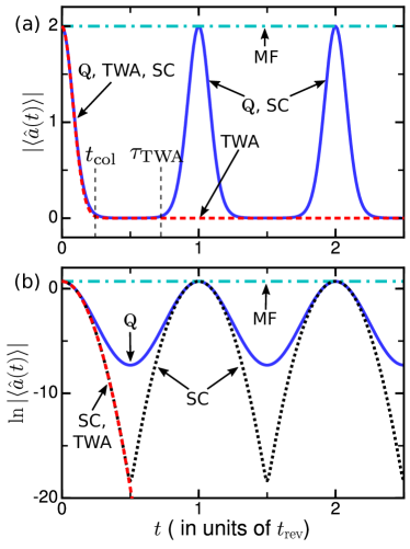
Figure 2: Collapse and revival in a nonlinear oscillator. Panels (a) and (b) show $|\left\langle a(t)\right\rangle|$ and $\ln|\left\langle a(t)\right\rangle|$, respectively, as a function of time $t$ for an initial coherent state whose mean atom number is four. Exact quantum dynamics (labeled Q) displays collapse and revival of $|\left\langle a(t)\right\rangle|$ with collapse and revival times $t_{\rm col}$ and $t_{\rm rev}$, respectively. The mean-field solution, labeled MF, is time independent. The TWA result, Eq. 24, closely replicates the first collapse but shows no revival and deviates appreciably from the quantum dynamics after a time $\tau_{\rm TWA}$. On the other hand, the semiclassical approximation (labeled SC), Eq. 27, agrees well with the quantum evolution for all times. In panel (a) the semiclassical and quantum curves are indistinguishable.

The nonlinear oscillator has been studied in experiments with a BEC in an optical lattice Greiner et al. (2002) and with photons using Kerr nonlinearity Kirchmair et al. (2013). In these experiments, the initial state is well-described by a coherent state, $\left|\psi_{0}\right\rangle=e^{-|\alpha|^{2}/2}\sum_{n=0}^{\infty}\alpha^{n}/\sqrt{n!}\left|n\right\rangle$, where $\alpha$, in general, is a complex number and $|\alpha|^{2}=N$ is the average number of atoms or photons. Using interference, the collapse and revival of the absolute value of the expectation value of $\hat{a}$ and a generalized Husimi function, respectively, were measured in these experiments. We find that the expectation value of $\hat{a}$ evolves as

$$\left\langle\hat{a}(t)\right\rangle=\left\langle\psi(t)|\hat{a}|\psi(t)\right\rangle =\alpha e^{|\alpha|^{2}(e^{-iUt/\hbar}-1)}.$$ (19)

Its absolute value is shown in Fig. 2. At short times $Ut/\hbar\ll 1$,

$$\left\langle\hat{a}(t)\right\rangle\approx\alpha e^{-|\alpha|^{2}U^{2}t^{2}/(2\hbar^{2})-iU|\alpha|^{2}t/\hbar},$$ (20)

whose decay in time is Gaussian with time constant $\hbar/(U\sqrt{N})$. The collapse time $t_{\rm col}$ is a few times this time constant, as shown in Fig. 2, and is much smaller $t_{\rm rev}$ for large $N$. In the experiments with a BEC in an optical lattice, three-body effects proportional to $(\hat{a}^{\dagger})^{3}\hat{a}^{3}$ change the nature of the collapse and revival in an interesting manner Johnson et al. (2009); Will et al. (2010); Tiesinga and Johnson (2011).

V.1 Dynamics according to the TWA

Next, we study the time dynamics of $\left\langle\hat{a}(t)\right\rangle$ within the TWA. First, we need to write down the classical Hamiltonian corresponding to $\hat{H}_{\rm NO}$ . It is

$$\mathcal{H}_{\rm NO}=\frac{U}{8\hbar^{2}}(x^{2}+p^{2})^{2}$$ (21)

with classical equations of motion

$$\frac{dx}{dt}=\frac{\partial\mathcal{H}_{\rm NO}}{\partial p}=\frac{U}{2\hbar^{2}}\rho^{2}p\,,\quad\frac{dp}{dt}=-\frac{\partial\mathcal{H}_{\rm NO}}{\partial x}=-\frac{U}{2\hbar^{2}}\rho^{2}x,$$ (22)

where $\rho^{2}=x^{2}+p^{2}$. Hence, classical paths lie on circles in phase space centered around the origin $(x,p)=(0,0)$. Their oscillation frequencies are $\omega=U\rho^{2}/(2\hbar^{2})$. The system is integrable as the phase space is two-dimensional and energy is conserved. The angle of the action-angle coordinates is the polar angle $\varphi$ measured in clockwise direction of motion and evolves as $\varphi(t)=\omega t+\varphi_{i}$, where $\varphi_{i}$ is the initial angle. Using the definition $\omega=\partial\mathcal{H}_{\rm NO}/\partial I$, we find that the action coordinate $I=\rho^{2}/2$. Hence, $\rho$ is a constant of motion.

For concreteness, let the initial coherent state $\left|\psi_{0}\right\rangle$, with occupation number $N\gg 1$, be centered along the $p$-axis, i.e., $\alpha=i\sqrt{N}$. Its Wigner distribution

$$W_{0}(x,p)=\frac{1}{\pi\hbar}e^{-\left[x^{2}+(p-\sqrt{2\hbar N})^{2}\right]/\hbar},$$ (23)

is centered at $(x,p)=(0,\sqrt{2\hbar N})$ and width $O(\sqrt{\hbar})$. Next, we calculate $\left\langle\hat{a}(t)\right\rangle_{\rm TWA}$, the expectation value of $\hat{a}$ within the TWA. Instead of using the Green’s function $G_{\rm TWA}$ of Eq. 14, it is more convenient to work in the Heisenberg picture. In this picture, the Wigner-Weyl transform of the operator $\hat{a}(t)$ is $a(t)=[x(t)+ip(t)]/\sqrt{2\hbar}=i\rho e^{-i\varphi(t)}/\sqrt{2\hbar}$ with $\varphi\in(-\pi,\pi]$ and $\varphi=0$ along the $p$-axis. Then using Eq. 4 and writing $W_{0}(x,p)$ in polar coordinates, we find

$$\left\langle\hat{a}(t)\right\rangle_{\rm TWA} =\int_{0}^{\infty}\rho d\rho\int_{-\pi}^{\pi}d\varphi_{i}\,\frac{i\rho}{\sqrt{2\hbar}}e^{-i\varphi(t)}W_{0}(\rho,\varphi_{i}).$$ (24)

For $N\gg 1$, it is sufficient to expand the exponent of $W_{0}(x,p)$ to second order in $\rho$ and $\varphi$ around the location of the maximum of the Wigner distribution, i.e.,

$$W_{0}(\rho,\varphi_{i})\approx\frac{1}{\pi\hbar}e^{-\left[(\rho-\sqrt{2\hbar N})^{2}-2\hbar N\varphi_{i}^{2}\right]/\hbar}.$$ (25)

Substituting this expression and $\omega=U\rho^{2}/(2\hbar)$ in Eq. 24, we derive

$$\left\langle\hat{a}(t)\right\rangle_{\rm TWA} \approx i\sqrt{N}e^{-U^{2}Nt^{2}/(2\hbar)-iUNt/\hbar},$$ (26)

which matches the initial collapse of the coherent state in Eq. 20, but has no revival. A comparison of Eq. 26 with the exact quantum result of Eq. 19 for the absolute value of $\left\langle\hat{a}(t)\right\rangle$ is shown in Fig. 2. The figure also shows the mean-field value $|\left\langle\hat{a}(t)\right\rangle_{\rm MF}|$, which is $|a(t)|$ along the single circular trajectory starting from $(x,p)=(0,\sqrt{2\hbar N})$. Thus, $|\left\langle\hat{a}(t)\right\rangle_{\rm MF}|=\sqrt{N}$ is a constant.

The classical phenomenon of phase-space mixing explains the collapse of $\left\langle\hat{a}(t)\right\rangle$ Mathew and Tiesinga (2017). For an integrable system, the coarse-grained long-time Wigner distribution is uniformly distributed in the angle coordinates of the action-angle variables. For the nonlinear oscillator, $a(t)\propto e^{i\varphi(t)}$ and its expectation value goes to zero as the Wigner distribution mixes in the angle $\varphi$. Furthermore, within the TWA, the coarsened Wigner distribution reaches a steady state; hence, there is no revival. This latter observation indicates that quantum interference reverses phase-space mixing and revives the quantum state. In the next section, we find that applying the semiclassical formalism, indeed, leads to revival.

V.2 Dynamics according to the semiclassical approximation

The calculation of $\left\langle\hat{a}(t)\right\rangle_{\rm SC}$ according to the semiclassical approximation is lengthy and has been relegated to Appendices B and C. We first calculate the action in terms of the polar angles and winding number of classical paths around the origin in Appendix B. We carry out the remainder the calculation in Appendix C. Here, we list the main steps:

1. The time evolution of an observable with Weyl symbol $\mathcal{O}(x,p)$ in the Schrödinger picture is given by Eq. 3. We replace $G(r_{f},r_{i},t)$ by $G_{\rm SC}(r_{f},r_{i},t)$ as given in Eq. 13 and carry out the integrals over $p_{i}$ and $p_{f}$ to arrive at Eq. 1.

2. The classical equations of motion are simplest in the action-angle coordinates. Therefore, we convert the integrals over $x_{i}$, $x_{f}$ and the double sum over $b$, $b^{\prime}$ in Eq. 1 into integrals over the initial and final angles $\varphi_{i}$ and $\varphi_{f}$, respectively, and a double sum over winding numbers of classical paths around the origin. We also express the observable, $G_{\rm SC}(r_{f},r_{i},t)$, and the initial Wigner distribution in terms of $\varphi_{i}$, $\varphi_{f}$ and winding numbers.

3. Next, we note that the classical motion in the phase space is restricted in an annulus of radius $\sqrt{2N}$ and width of $O(1)$. Then, $\mathcal{O}(x,p)\approx\mathcal{O}(\sqrt{2N}\sin\varphi,\sqrt{2N}\cos\varphi)$; in particular, $a(x,p)\approx i\sqrt{N}e^{-i\varphi}$. We make similar approximations for the determinants $\mathcal{D}^{b}(x_{f},x_{i},t)$. The initial Wigner distribution, however, varies sharply with $\rho$ and requires a more careful approximation. We then solve the remaining integrals.

Finally, we find

$$\left\langle\hat{a}(t)\right\rangle_{\rm SC}=\sum_{v=-\infty}^{\infty}i\sqrt{N}e^{-iUNt/\hbar}e^{-\left(2\pi v-Ut/\hbar\right)^{2}N/2},$$ (27)

where $v$ is difference of the winding number of the interfering paths. This expression corresponds to a train of localized Gaussians and is invariant under the transformation $t\to t+2\pi\hbar/U$ and $v\to v-1$; hence, is periodic with time period $t_{\rm rev}=2\pi\hbar/U$. Figure 2 shows that $\left\langle\hat{a}(t)\right\rangle_{\rm SC}$ agrees with the exact quantum average $\left\langle\psi(t)|\hat{a}|\psi(t)\right\rangle$ for all times.

Finally, we discuss the Ehrenfest times of the nonlinear oscillator for initial coherent states. From Fig. 2(a), we see that the mean-field prediction deviates from the quantum evolution well before the collapse time $t_{\rm col}$, i.e., $\tau_{\rm MF}<t_{\rm col}$. In contrast, the deviation of the TWA from quantum evolution (ignoring exponentially small differences) occurs abruptly after a finite time $\tau_{\rm TWA}=t_{\rm rev}-t_{\rm col}$ before the first revival of $\left\langle\hat{a}(t)\right\rangle$. The interference of classical paths starts at $\tau_{\rm inter}$ when the Wigner distribution fills up the annular accessible phase space, i.e., when paths starting from the initial localized distribution with winding numbers zero and one terminate in the same small region of phase space. We can estimate $\tau_{\rm inter}$ by noting that for a coherent state the distribution of classical frequencies $\omega$ has a mean $UN/\hbar$ and width $\Delta\omega=U\sqrt{N}/\hbar$. Therefore, $\tau_{\rm inter}\sim 2\pi/\Delta\omega$ is of the order of $t_{\rm col}$ and, hence, is much smaller than $\tau_{\rm TWA}$. In other words, it takes time for the interference of paths to affect $\left\langle\hat{a}(t)\right\rangle$ appreciably. In fact, at $\tau_{\rm TWA}$ the number of interfering classical paths is of the order of $\sqrt{N}$. On the other hand, the Ehrenfest time $\tau_{\rm SC}$ is infinite for the nonlinear oscillator.

The Ehrenfest time $\tau_{\rm TWA}$ depends on the observable under consideration. For example, for $\left\langle\hat{a}^{2}(t)\right\rangle$ the collapse and revival times are $t_{\rm rev}/2$ and $t_{\rm col}/2$, respectively, and the TWA fails after $(t_{\rm rev}-t_{\rm col})/2$. Nevertheless, $\tau_{\rm TWA}$ is still greater than $\tau_{\rm inter}$ for all observables (that are polynomials in $a$ and $a^{\dagger}$ with a degree smaller than $N$). We also expect the delay in effects of interference and the dependence of $\tau_{\rm TWA}$ on the observable to hold true for generic integrable systems (where the dynamics is away from singularities like a saddle point of the classical Hamiltonian). In contrast, in a chaotic system and for motion near a saddle point of an integrable system, the Ehrenfest time $\tau_{\rm TWA}\sim\tau_{\rm inter}$ Aleiner and Larkin (1996); Rozenbaum et al. (2017); Mathew and Tiesinga (2017).

VI Conclusion and outlook

In conclusion, we presented a semiclassical theory of phase-space dynamics of bosons. We derived a semiclassical approximation, Eq. 10, to the exact Green’s function of the Wigner distribution. Crucially, the approximation preserves the quantum interference of classical trajectories. In fact, we have shown that the formalism reduces to the TWA when the interference terms are ignored. Hence, the Ehrenfest time associated with the breakdown of the TWA occurs when interference of classical paths becomes important. As a case study, we examined a single-mode nonlinear oscillator whose exact quantum dynamics exhibits collapse and revival. We investigated the dynamics of an observable of this oscillator using the TWA and our semiclassical formalism. Within TWA, the expectation value of an observable collapses due to phase mixing, and there is no revival. The semiclassical approximation, however, reproduces revivals and accurately matches the exact quantum dynamics for all times.

Finally, we comment on the long-time validity of our semiclassical approximation. For the nonlinear oscillator, the semiclassical approach is valid for all times . We expect this to be true for generic integrable systems as they can be quantized by the Einstein-Brillouin-Keller method Keller (1958). The situation, however, is not straightforward for chaotic systems. For example, the semiclassical evolution (based on the van Vleck-Gutzwiller propagator) of an initial wavefunction defined on a Lagrangian manifold, whose Wigner distribution is not localized, breaks down after a time of the order of the Ehrenfest time associated with interference of classical paths Berry (1979); Berry et al. (1979). For localized initial Wigner distributions, however, numerical studies and heuristic arguments have shown that the van Vleck-Gutzwiller propagator works for rather longer times Tomsovic and Heller (1993); Dittes et al. (1994); Heller and Tomsovic (1993) and only breaks down due to diffraction. The validity of our semiclassical approach for chaotic systems will require further study.

Appendix A Derivatives of action

We evaluate the partial derivatives of the action $S^{b}(\mathbf{x}_{f},\mathbf{x}_{i},t)$ with respect to the initial and final positions. The action satisfies the Hamilton-Jacobi equation and, in principle, its derivates are well known Goldstein (1980); Arnold (1997). Here, we give a derivation for the sake of completeness. For notational simplicity, we assume that the configuration space is one-dimensional; generalization to higher dimensions is straightforward. Consider a classical path $[x^{b}_{\rm cl}(\tau),p^{b}_{\rm cl}(\tau)]$, which starts from the phase-space point $(x_{i},p^{b}_{i})$ and ends at $(x_{f},p^{b}_{f})$. Next, consider another classical path whose position in time, $x_{\rm cl}^{b}(\tau)+\delta x_{\rm cl}^{b}(\tau)$, is infinitesimally close to $x_{\rm cl}^{b}(\tau)$ such that $\delta x_{\rm cl}^{b}(0)=\Delta x_{i}$ and $\delta x_{\rm cl}^{b}(t)=0$. Then the change in the action is

$$\Delta S^{b} =\int_{0}^{t}d\tau\,\left(\frac{\partial L}{\partial x_{\rm cl}}\delta x_{\rm cl}^{b}(\tau)+\frac{\partial L}{\partial\dot{x}_{\rm cl}}\delta\dot{x}_{\rm cl}^{b}(\tau)\right)$$

$$=\frac{\partial L}{\partial\dot{x}_{\rm cl}}\delta x_{\rm cl}^{b}(\tau)\bigg{\rvert}_{0}^{t}+\int_{0}^{t}dt\,\left(\frac{\partial L}{\partial x_{\rm cl}}-\frac{d}{dt}\frac{\partial L}{\partial\dot{x}_{\rm cl}}\right)\delta x_{\rm cl}^{b}(\tau),$$

where $\dot{x}_{\rm cl}=dx_{\rm cl}/d\tau$ and we have suppressed the arguments of $L$. Now, the second term vanishes because $x_{\rm cl}^{b}(\tau)$ satisfies the Euler-Lagrange equations of motion. Using the fact that $p=\partial L(x,\dot{x})/\partial\dot{x}$, we have $\Delta S^{b}=-p^{b}_{i}\Delta x_{i}$ or

$$\frac{\partial S^{b}(x_{f},x_{i},t)}{\partial x_{i}}=-p^{b}_{i}.$$ (28)

Similarly, we can prove that

$$\frac{\partial S^{b}(x_{f},x_{i},t)}{\partial x_{f}}=p^{b}_{f}.$$ (29)

Appendix B Action of the nonlinear oscillator

We compute the action $S^{b}(x_{f},x_{i},t)$ of the nonlinear oscillator described in Sec. V. The action depends on the index $b$, which we have not yet quantified. A natural guess is the winding number $w$ of a circular path around the phase-space origin. The winding number is a nonnegative integer as the motion in phase space is unidirectional. For a given $(x_{f},x_{i},w,t)$, however, more than one classical path can exist. For example, two such paths are shown in Fig. 3. In contrast, a given $(\varphi_{f},\varphi_{i},w,t)$, where $\varphi_{i}$ and $\varphi_{f}$ are the initial and final angles, respectively, uniquely determines a classical path. The reason is that the oscillation frequency is specified by

$$\omega=\frac{(\varphi_{f}-\varphi_{i})\bmod 2\pi+2\pi w}{t}$$ (30)

and, hence, uniquely determines the radius $\rho=\hbar\sqrt{2\omega/U}$ (see Sec. V.1) of the classical path.

It is convenient to define the action $\mathscr{S}^{w}(\varphi_{f},\varphi_{i},t)=S^{b}[x_{f}(\varphi_{f},\varphi_{i},w,t),x_{i}(\varphi_{f},\varphi_{i},w,t),t]$, indexed by the winding number $w$ of path $b$ and

$$\mathscr{S}^{w}(\varphi_{f},\varphi_{i},t) =\int_{0}^{t}d\tau\,\left[p_{\rm cl}\frac{dx_{\rm cl}}{d\tau}-\mathcal{H}_{\rm NO}\right],$$ (31)

where $\mathcal{H}_{\rm NO}$ is given by Eq. 21 and we have suppressed the arguments $(\varphi_{f},\varphi_{i},w,t)$. Substituting $x_{\rm cl}(\tau)=\rho\sin\varphi(\tau)$ and $p_{\rm cl}(\tau)=\rho\cos\varphi(\tau)$, we find

$$\mathscr{S}^{w}(\varphi_{f},\varphi_{i},t) =\int_{0}^{t}d\tau\,\left(\omega\rho^{2}\cos^{2}\varphi(\tau)-\frac{U\rho^{4}}{8}\right),$$

where we used $d\rho/d\tau=0$, $d\varphi/d\tau=\omega$ and have set $\hbar=1$. The integration over $\tau$ yields

$$\mathscr{S}^{w}(\varphi_{f},\varphi_{i},t)=\frac{[(\varphi_{f}-\varphi_{i})\bmod{2\pi}+2\pi w]}{2Ut}$$

$$\times\left[(\varphi_{f}-\varphi_{i})\bmod{2\pi}+2\pi w+\sin(2\varphi_{f})-\sin(2\varphi_{i})\right].$$

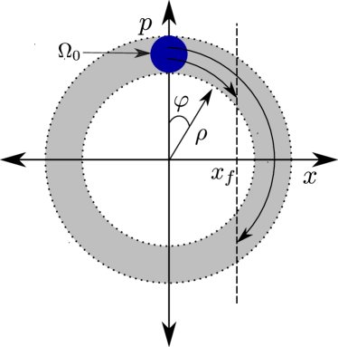
Figure 3: Classical paths of a nonlinear oscillator in phase space $(x,p)$ starting from a Wigner distribution initially localized in region $\Omega_{0}$ shown by the solid blue circle. Polar coordinates $(\rho,\varphi)$, with angle $\varphi$ measured from the $p$-axis in a clockwise direction, are also shown. The region $\Omega_{0}$ is centered at $(\rho,\varphi)=(\sqrt{2N},0)$ and has a width of $O(1)$. Trajectories starting from $\Omega_{0}$ lie within the gray annulus. Two paths with traversal time $t$ and winding number zero that start from $x=0$ and end at $x=x_{f}$ are shown.

Appendix C Calculation of $\left\langle\hat{a}(t)\right\rangle$

We calculate the expectation value of $\hat{a}(t)$ within the semiclassical approximation and follow the outline presented in Sec. V.2.

1. The semiclassical evolution of the expectation value of an observable of the nonlinear oscillator $\hat{\mathcal{O}}$ with Weyl symbol $\mathcal{O}(x,p)$ is

   $$\left\langle\hat{\mathcal{O}}(t)\right\rangle_{\rm SC} =\int dr_{i}dr_{f}\,\mathcal{O}(r_{f})G_{\rm SC}(r_{f},r_{i},t)W_{0}(r_{i}).$$ (33)

   Substituting $G_{\rm SC}(r_{f},r_{i},t)$ from Eq. 10 and integrating over the momenta $p_{i}$ and $p_{f}$, we find

   $$\left\langle\hat{\mathcal{O}}(t)\right\rangle_{\rm SC}=\int dx_{i}dx_{f}\,\sum_{b,b^{\prime}}\mathcal{O}\left(x_{f},\frac{p^{b}_{f}+p^{b^{\prime}}_{f}}{2}\right)$$

   $$\times W_{0}\left(x_{i},\frac{p^{b}_{i}+p^{b^{\prime}}_{i}}{2}\right)\sqrt{\mathcal{D}^{b}\mathcal{D}^{b^{\prime}}}\,e^{iS^{b}-iS^{b^{\prime}}-i(\mu^{b}-\mu^{b^{\prime}})\pi/2},$$

   where we suppress the dependence of $p_{i}^{b}$, $\mathcal{D}^{b}$, $S^{b}$, etc., on $(x_{f},x_{i},t)$ and set $\hbar=1$. The range of integration is $(-\infty,\infty)$ for both $x_{i}$ and $x_{f}$.

2. The action has a simpler form in terms of the angles (see Eq. B). Hence, we proceed to change the integration variables in Eq. 1 to the angle coordinates. To this end, we first introduce a set of initial and final positions $x^{\prime}_{i}$ and $x^{\prime}_{f}$, respectively, and write a symmetric expression

   $$\left\langle\mathcal{O}(t)\right\rangle_{\rm SC} =\int dx_{i}dx_{f}dx^{\prime}_{i}dx^{\prime}_{f}\,\delta(x_{i}-x^{\prime}_{i})\delta(x_{f}-x^{\prime}_{f})$$ (35)

   $$\times\sum_{b,b^{\prime}}\mathcal{O}\left[\frac{x_{f}+x^{\prime}_{f}}{2},\frac{p^{b}_{f}(x_{f},x_{i},t)+p^{b^{\prime}}_{f}(x^{\prime}_{f},x^{\prime}_{i},t)}{2}\right]W_{0}\left[\frac{x_{i}+x^{\prime}_{i}}{2},\frac{p^{b}_{i}(x_{f},x_{i},t)+p^{b^{\prime}}_{i}(x^{\prime}_{f},x^{\prime}_{i},t)}{2}\right]$$

   $$\times\sqrt{\mathcal{D}^{b}(x_{f},x_{i},t)\mathcal{D}^{b^{\prime}}(x^{\prime}_{f},x^{\prime}_{i},t)}\,e^{iS^{b}(x_{f},x_{i},t)-iS^{b^{\prime}}(x^{\prime}_{f},x^{\prime}_{i},t)-i[\mu^{b}(x_{f},x_{i},t)-\mu^{b^{\prime}}(x^{\prime}_{f},x^{\prime}_{i},t)]\pi/2},$$

   where the explicit dependence of the quantities is shown to avoid any confusion. The two sets of paths indexed by $b$ and $b^{\prime}$ now have different boundary conditions $(x_{f},x_{i},t)$ and $(x^{\prime}_{f},x^{\prime}_{i},t)$, respectively, enabling us to interchange the sum over $b$ and integrals over $x^{\prime}_{i}$ and $x^{\prime}_{f}$. The next step is to change the integration measure in terms of one for the angles. This step is carried out in Appendix  C.1 and we find

   $$\int dx_{i}dx_{f}\sum_{b}(\dots) =\sum_{w=w_{\rm min}}^{w_{\rm max}}\int_{-\pi}^{\pi}d\varphi_{f}\int_{-\pi}^{\pi}d\varphi_{i}\,|\det J|\,(\dots),$$ (36)

   where $(\dots)$ is a function of $(x_{f},x_{i},b,t)$ and the Jacobian matrix $J=\partial(x^{w}_{i},x^{w}_{f})/\partial(\varphi_{i},\varphi_{f})$ with $x^{w}_{i}=x_{i}(\varphi_{f},\varphi_{i},w,t)$ and $x^{w}_{f}=x_{f}(\varphi_{f},\varphi_{i},w,t)$. The nonnegative integers $w_{\rm min}$ and $w_{\rm max}$ are minimum and maximum winding numbers, respectively, of trajectories starting from region $\Omega_{0}$, as shown in Fig. 3. An equation analogous to Eq. 36 holds for measures of $x^{\prime}_{i}$ and $x^{\prime}_{f}$. Substitution of these measure changes in Eq. 35 yields

   $$\left\langle\mathcal{O}(t)\right\rangle_{\rm SC} =\sum_{w,w^{\prime}=w_{\rm min}}^{w_{\rm max}}\int d\varphi_{i}d\varphi_{f}d\varphi^{\prime}_{i}d\varphi^{\prime}_{f}\,\left|\det\left[\frac{\partial(x^{w}_{i},x^{w}_{f})}{\partial(\varphi_{i},\varphi_{f})}\right]\right|\left|\det\left[\frac{\partial(x^{w^{\prime}}_{i},x^{w^{\prime}}_{f})}{\partial(\varphi^{\prime}_{i},\varphi^{\prime}_{f})}\right]\right|\delta(x_{i}^{w}-x_{i}^{w^{\prime}})\delta(x_{f}^{w}-x_{f}^{w^{\prime}})$$

   $$\quad\times\mathcal{O}\left(\frac{x^{w}_{f}+x^{w^{\prime}}_{f}}{2},\frac{p^{w}_{f}+p^{w^{\prime}}_{f}}{2}\right)W_{0}\left(\frac{x^{w}_{i}+x^{w^{\prime}}_{i}}{2},\frac{p^{w}_{i}+p^{w^{\prime}}_{i}}{2}\right)\sqrt{\mathscr{D}^{w}\mathscr{D}^{w^{\prime}}}\,e^{i\mathscr{S}^{w}-i\mathscr{S}^{w^{\prime}}-i(\mu^{w}-\mu^{w^{\prime}})\pi/2},$$ (37)

   where the arguments of quantities with superscript $w$ and $w^{\prime}$ are $(\varphi_{i}$, $\varphi_{f},t)$ and $(\varphi^{\prime}_{i}$, $\varphi^{\prime}_{f},t)$, respectively. Moreover, we have introduced $\mathscr{D}^{w}(\varphi_{f},\varphi_{i},t)=\mathcal{D}^{b}(x^{w}_{f},x^{w}_{i},t)$ and $\mathscr{S}^{w}(\varphi_{f},\varphi_{i},t)$ is given by Eq. B.

3. We explicitly write all quantities appearing in Eq. 37 in terms of $(\varphi_{f},\varphi_{i},w,t)$. We do so by noting that the relevant classical motion is restricted in an annulus of width $O(1)$ around $\rho=\sqrt{2N}$ (see Fig. 3). In the annulus, we approximate the radius by its mean $\sqrt{2N}$, i.e., $x^{w}_{i}\approx\sqrt{2N}\sin\varphi_{i}$, $p^{w}_{i}\approx\sqrt{2N}\sin\varphi_{i}$, etc., which leads to

   $$\left|\det\left[\frac{\partial(x^{w}_{i},x^{w}_{f})}{\partial(\varphi_{i},\varphi_{f})}\right]\right|\approx 2N|\cos\varphi_{i}\cos\varphi_{f}|$$ (38)

   and

   $$\mathscr{D}^{w}(\varphi_{f},\varphi_{i},t)\approx\frac{1}{2UNt|\cos\varphi_{i}\cos\varphi_{f}|},$$ (39)

   etc. Moreover, as the initial Wigner distribution is localized around angle $\varphi=0$, $\delta(x_{i}^{w}-x_{i}^{w^{\prime}})\approx\delta(\varphi_{f}-\varphi_{f}^{\prime})/(\sqrt{2N}\cos\varphi_{f}).$ The other delta function becomes

   $$\delta(x_{f}^{w}-x_{f}^{w^{\prime}}) \approx\frac{\delta(\varphi_{f}-\varphi_{f}^{\prime})+\delta(\varphi_{f}+\varphi_{f}^{\prime}-\pi)}{\sqrt{2N}\cos\varphi_{f}}.$$ (40)

   The two contributions reflect the fact that a line at fixed value of $x_{f}$ intersects the thin annulus in two regions, whose respective angles are approximated by the angle of the intersection with the circle of radius $\rho=\sqrt{2N}$.

   Substituting these approximations into Eq. 37 and integrating over $\varphi^{\prime}_{i}$ and $\varphi^{\prime}_{f}$, we find

   $$\left\langle\mathcal{O}(t)\right\rangle_{\rm SC}=\frac{1}{Ut}\sum_{w,w^{\prime}=w_{\rm min}}^{w_{\rm max}}\int d\varphi_{i}d\varphi_{f}\,\mathcal{O}\,W_{0}$$ (41)

   $$\times\,e^{i\mathscr{S}^{w}-i\mathscr{S}^{w^{\prime}}-i(\mu^{w}-\mu^{w^{\prime}})\pi/2},$$

   where we suppress the arguments of $\mathcal{O}$ and $W_{0}$, and neglect the contribution from the second term in Eq. 40. This term leads to a highly oscillating integrand whose integral is small. The arguments of quantities in the integrand with either superscript $w$ or $w^{\prime}$ are now $\varphi_{f}$, $\varphi_{i}$ and $t$.

   Next, we note that $\mathcal{O}(x,p)$ is a slowly varying function of $x,p$ and within the annulus $\mathcal{O}\left[\tfrac{1}{2}\left(x^{w}_{f}+x^{w^{\prime}}_{f}\right),\tfrac{1}{2}\left(p^{w}_{f}+p^{w^{\prime}}_{f}\right)\right]\approx\mathcal{O}(\sqrt{2N}\sin\varphi_{f},\sqrt{2N}\cos\varphi_{f})$. In particular,

   $$a\left[\tfrac{1}{2}\left(x^{w}_{f}+x^{w^{\prime}}_{f}\right),\tfrac{1}{2}\left(p^{w}_{f}+p^{w^{\prime}}_{f}\right)\right]\approx i\sqrt{N}e^{-i\varphi_{f}}.$$ (42)

   We cannot make a similar approximation for the initial Wigner distribution, i.e., replace $\rho^{w}$ and $\rho^{w^{\prime}}$ by $\sqrt{2N}$, because the distribution varies sharply around $\rho=\sqrt{2N}$. Instead, we write

   $$\frac{\rho^{w}(\varphi_{f},\varphi_{i},t)}{\sqrt{2N}}=\left[\frac{(\varphi_{f}-\varphi_{i})\bmod 2\pi+2\pi w}{UNt}\right]^{1/2}$$ (43)

   $$\approx 1+\frac{1}{2}\left[\frac{(\varphi_{f}-\varphi_{i})\bmod 2\pi+2\pi w}{UNt}-1\right],$$

   where we used the relation $\rho=\sqrt{2\omega/U}$ (see Sec. V.1), Eq. 30 and performed a Taylor expansion around $\rho^{w}/\sqrt{2N}=1$. We substitute $\rho$ in the initial Wigner distribution of Eq. 25 by the Taylor approximation for $(\rho^{w}+\rho^{w^{\prime}})/2$, to find

   $$W_{0}\left(\frac{x^{w}_{i}+x^{w^{\prime}}_{i}}{2},\frac{p^{w}_{i}+p^{w^{\prime}}_{i}}{2}\right)\approx$$

   $$\frac{1}{\pi}e^{-\left[(\varphi_{f}-\varphi_{i})\bmod 2\pi+\pi(w+w^{\prime})-UNt\right]^{2}/{2U^{2}Nt^{2}}-2N\varphi_{i}^{2}}\,.$$

   Also, from Eq. B, we have

   $$\mathscr{S}^{w}-\mathscr{S}^{w^{\prime}} =\frac{2\pi}{Ut}(w-w^{\prime})[(\varphi_{f}-\varphi_{i})\bmod 2\pi+\pi(w+w^{\prime})]$$ (45)

   Finally, the Maslov index, which is the number of turning points of a classical path, increases by two for every winding. Therefore,

   $$\mu^{w}-\mu^{w^{\prime}}=2(w-w^{\prime}).$$ (46)

   After substituting $\mathcal{O}(x,p)=a(x,p)$, Eqs. 42, 3, 45, and 46 in Eq. 41, we find

   $$\left\langle a(t)\right\rangle_{\rm SC} =\frac{i\sqrt{N}}{\pi Ut}\sum_{w,w^{\prime}=w_{\rm min}}^{w_{\rm max}}\int_{-\pi}^{\pi}d\varphi_{i}\int_{-\pi}^{\pi}d\varphi_{f}\,e^{-i\varphi_{f}-i(w-w^{\prime})\pi}\,e^{-\left[(\varphi_{f}-\varphi_{i})\bmod 2\pi+\pi(w+w^{\prime})-UNt\right]^{2}/(2U^{2}Nt^{2})}$$

   $$\quad\times e^{-2N\varphi_{i}^{2}}e^{i2\pi(w-w^{\prime})[(\varphi_{f}-\varphi_{i})\bmod 2\pi+\pi(w+w^{\prime})]/(Ut)}.$$ (47)

   Next, we extend the limits on $w$ and $w^{\prime}$ to $[0,\infty)$ and write the sums over $w$ and $w^{\prime}$ in terms of $u=w+w^{\prime}$ and $v=w-w^{\prime}$. We combine the sum over $u$ and the integral over $\varphi_{f}$ by defining $y=(\varphi_{f}-\varphi_{i})\bmod 2\pi+\pi u$, whose range is $[0,\infty)$. We realize that $e^{-i\varphi_{f}-i(w-w^{\prime})\pi}=e^{-i(y+\varphi_{i})}$ and the integrand is separable in $\varphi_{i}$ and $y$. After evaluating the integrals, we arrive at

   $$\left\langle a(t)\right\rangle_{\rm SC} =\sum_{v=-\infty}^{\infty}i\sqrt{N}e^{-iUNt}e^{-\left(2\pi v-Ut\right)^{2}N/2}e^{-1/(8N)}$$

   which becomes Eq. 27 of the main text for large $N$.

C.1 Derivation of Eq. 36

Here, we derive Eq. 36. We restrict our attention to paths that start from the phase-space region $\Omega_{0}$, in which the initial Wigner distribution is concentrated. Figure 3 shows the region $\Omega_{0}$ for the nonlinear oscillator. The paths starting within $\Omega_{0}$ lie on the annulus shown in the figure. Now, the winding number of a circular path at a fixed traversal time is a stepwise increasing function of the radius. Let the (time-dependent) winding numbers of paths that lie on the inner and outer circles of the annulus be $w_{\rm min}$ and $w_{\rm max}$, respectively, with $w_{\rm min}\leq w_{\rm max}$. For a given winding number, there can be two paths that start from $\Omega_{0}$ with position $x_{i}$ and reach position $x_{f}$ in time $t$. Figure 3 shows a pair of such paths with winding number zero and $x_{i}=0$. Moreover, the paths end in the upper ($p>0$) and lower ($p\leq 0$) halves of the phase space. Therefore, we can interchange the integrals over boundary conditions and sum over paths to find

$$\int dx_{i}dx_{f}\sum_{b}\left(\dots\right)=\sum_{\begin{subarray}{c}w=w_{\rm min},{\,\rm upper}\end{subarray}}^{w_{\rm max}}\int dx_{i}dx_{f}(\dots)\\ +\sum_{\begin{subarray}{c}w=w_{\rm min},{\,\rm lower}\end{subarray}}^{w_{\rm max}}\int dx_{i}dx_{f}(\dots),$$ (48)

where the labels “upper” and “lower” indicate paths that end in the corresponding half of phase space.

In each half of the phase space, the final angle is uniquely determined given $(x_{f},x_{i},w,t)$. Therefore, we can transform the integrals over $x_{i}$ and $x_{f}$ in Eq. 48 to one over angles and combine the “upper” and “lower” contributions to arrive at Eq. 36.

$\square$

References

- Feynman et al. (1963) R. Feynman, R. Leighton, and M. Sands, The Feynman Lectures on Physics, no. v. 3 in The Feynman Lectures on Physics (Pearson/Addison-Wesley, 1963).
- Schulman (2005) L. S. Schulman, Techniques and applications of path integration (Dover Publications, 2005).
- Morette (1951) C. Morette, Physical Review 81, 848 (1951), URL https://link.aps.org/doi/10.1103/PhysRev.81.848.
- Vleck (1928) J. H. V. Vleck, Proceedings of the National Academy of Sciences 14, 178 (1928), ISSN 0027-8424, 1091-6490, URL http://www.pnas.org/content/14/2/178.
- Gutzwiller (1971) M. C. Gutzwiller, Journal of Mathematical Physics 12, 343 (1971), ISSN 0022-2488, URL http://aip.scitation.org/doi/abs/10.1063/1.1665596.
- Pechukas (1969) P. Pechukas, Physical Review 181, 166 (1969), URL https://link.aps.org/doi/10.1103/PhysRev.181.166.
- Rammer (2004) J. Rammer, Quantum transport theory, vol. 99 (Westview Press, 2004).
- Brouwer and Altland (2008) P. W. Brouwer and A. Altland, Physical Review B 78, 075304 (2008), URL https://link.aps.org/doi/10.1103/PhysRevB.78.075304.
- Tian et al. (2005) C. Tian, A. Kamenev, and A. Larkin, Physical Review B 72, 045108 (2005), URL https://link.aps.org/doi/10.1103/PhysRevB.72.045108.
- Aleiner and Larkin (1997) I. L. Aleiner and A. I. Larkin, Physical Review E 55, R1243 (1997), URL http://link.aps.org/doi/10.1103/PhysRevE.55.R1243.
- Müller et al. (2005) S. Müller, S. Heusler, P. Braun, F. Haake, and A. Altland, Physical Review E 72, 046207 (2005), URL https://link.aps.org/doi/10.1103/PhysRevE.72.046207.
- Jarzynski et al. (2015) C. Jarzynski, H. Quan, and S. Rahav, Physical Review X 5, 031038 (2015), URL https://link.aps.org/doi/10.1103/PhysRevX.5.031038.
- Wintgen et al. (1992) D. Wintgen, K. Richter, and G. Tanner, Chaos: An Interdisciplinary Journal of Nonlinear Science 2, 19 (1992), ISSN 1054-1500, URL http://aip.scitation.org/doi/abs/10.1063/1.165920.
- Richter and Richter (2000) K. Richter and K. Richter, Semiclassical theory of mesoscopic quantum systems, vol. 11 (Springer Berlin, 2000).
- Baranger et al. (1993) H. U. Baranger, R. A. Jalabert, and A. D. Stone, Physical Review Letters 70, 3876 (1993), URL https://link.aps.org/doi/10.1103/PhysRevLett.70.3876.
- Groenewold (1946) H. J. Groenewold, Physica 12, 405 (1946), ISSN 0031-8914, URL http://www.sciencedirect.com/science/article/pii/S0031891446800594.
- Moyal (1949) J. E. Moyal, Mathematical Proceedings of the Cambridge Philosophical Society 45, 99 (1949), ISSN 1469-8064, 0305-0041, URL https://www.cambridge.org/core/journals/mathematical-proceedings-of-the-cambridge-philosophical-society/article/quantum-mechanics-as-a-statistical-theory/9D0DC7453AD14DB641CF8D477B3C72A2.
- Curtright et al. (2014) T. L. Curtright, D. B. Fairlie, and C. K. Zachos, A concise treatise on quantum mechanics in phase space (World Scientific, 2014).
- Heller (1991) E. J. Heller, The Journal of Chemical Physics 94, 2723 (1991), ISSN 0021-9606, URL http://aip.scitation.org/doi/abs/10.1063/1.459848.
- Steel et al. (1998) M. J. Steel, M. K. Olsen, L. I. Plimak, P. D. Drummond, S. M. Tan, M. J. Collett, D. F. Walls, and R. Graham, Physical Review A 58, 4824 (1998), URL https://link.aps.org/doi/10.1103/PhysRevA.58.4824.
- Blakie et al. (2008) P. Blakie, A. Bradley, M. Davis, R. Ballagh, and C. Gardiner, Advances in Physics 57, 363 (2008), ISSN 0001-8732, URL http://www-tandfonline-com/doi/full/10.1080/00018730802564254.
- Polkovnikov (2003) A. Polkovnikov, Physical Review A 68, 053604 (2003), URL http://link.aps.org/doi/10.1103/PhysRevA.68.053604.
- Polkovnikov (2010) A. Polkovnikov, Annals of Physics 325, 1790 (2010), ISSN 0003-4916, URL http://www.sciencedirect.com/science/article/pii/S0003491610000382.
- Engl et al. (2014) T. Engl, J. Dujardin, A. Argüelles, P. Schlagheck, K. Richter, and J. D. Urbina, Physical Review Letters 112, 140403 (2014), URL https://link.aps.org/doi/10.1103/PhysRevLett.112.140403.
- Tomsovic et al. (2017) S. Tomsovic, P. Schlagheck, D. Ullmo, J. D. Urbina, and K. Richter, arXiv:1711.04693 [cond-mat, physics:quant-ph] (2017), arXiv: 1711.04693, URL http://arxiv.org/abs/1711.04693.
- Simon and Strunz (2014) L. Simon and W. T. Strunz, Physical Review A 89, 052112 (2014), URL https://link.aps.org/doi/10.1103/PhysRevA.89.052112.
- Ray et al. (2016) S. Ray, P. Ostmann, L. Simon, F. Grossmann, and W. T. Strunz, Journal of Physics A: Mathematical and Theoretical 49, 165303 (2016), ISSN 1751-8121, URL http://stacks.iop.org/1751-8121/49/i=16/a=165303.
- Hillery et al. (1984) M. Hillery, R. F. O’Connell, M. O. Scully, and E. P. Wigner, Physics Reports 106, 121 (1984), ISSN 0370-1573, URL http://www.sciencedirect.com/science/article/pii/0370157384901601.
- Berry et al. (1979) M. V. Berry, N. L. Balazs, M. Tabor, and A. Voros, Annals of Physics 122, 26 (1979), ISSN 0003-4916, URL http://www.sciencedirect.com/science/article/pii/0003491679902963.
- Marinov (1991) M. S. Marinov, Physics Letters A 153, 5 (1991), ISSN 0375-9601, URL http://www.sciencedirect.com/science/article/pii/0375960191903529.
- Dittrich et al. (2010) T. Dittrich, E. A. Gómez, and L. A. Pachón, The Journal of Chemical Physics 132, 214102 (2010), ISSN 0021-9606, 1089-7690, URL http://aip.scitation.org/doi/10.1063/1.3425881.
- Littlejohn (1992) R. G. Littlejohn, Journal of Statistical Physics 68, 7 (1992), ISSN 0022-4715, 1572-9613, URL https://link.springer.com/article/10.1007/BF01048836.
- Berman and Zaslavsky (1978) G. P. Berman and G. M. Zaslavsky, Physica A: Statistical Mechanics and its Applications 91, 450 (1978), ISSN 0378-4371, URL http://www.sciencedirect.com/science/article/pii/0378437178901905.
- Chirikov et al. (1988) B. V. Chirikov, F. M. Izrailev, and D. L. Shepelyansky, Physica D: Nonlinear Phenomena 33, 77 (1988), ISSN 0167-2789, URL http://www.sciencedirect.com/science/article/pii/S0167278998900112.
- Silvestrov and Beenakker (2002) P. G. Silvestrov and C. W. J. Beenakker, Physical Review E 65, 035208 (2002), URL https://link.aps.org/doi/10.1103/PhysRevE.65.035208.
- Tomsovic and Heller (2003) S. Tomsovic and E. J. Heller, Physical Review E 68, 038201 (2003), URL https://link.aps.org/doi/10.1103/PhysRevE.68.038201.
- Tomsovic and Heller (1993) S. Tomsovic and E. J. Heller, Physical Review E 47, 282 (1993), URL https://link.aps.org/doi/10.1103/PhysRevE.47.282.
- Dittes et al. (1994) F.-M. Dittes, E. Doron, and U. Smilansky, Physical Review E 49, R963 (1994), URL https://link.aps.org/doi/10.1103/PhysRevE.49.R963.
- Greiner et al. (2002) M. Greiner, O. Mandel, T. W. Hänsch, and I. Bloch, Nature 419, 51 (2002), ISSN 0028-0836, URL http://www.nature.com/nature/journal/v419/n6902/full/nature00968.html.
- Kirchmair et al. (2013) G. Kirchmair, B. Vlastakis, Z. Leghtas, S. E. Nigg, H. Paik, E. Ginossar, M. Mirrahimi, L. Frunzio, S. M. Girvin, and R. J. Schoelkopf, Nature 495, 205 (2013), ISSN 0028-0836, URL http://www.nature.com/nature/journal/v495/n7440/full/nature11902.html.
- Johnson et al. (2009) P. R. Johnson, E. Tiesinga, J. V. Porto, and C. J. Williams, New Journal of Physics 11, 093022 (2009), ISSN 1367-2630, URL http://stacks.iop.org/1367-2630/11/i=9/a=093022.
- Will et al. (2010) S. Will, T. Best, U. Schneider, L. Hackermüller, D.-S. Lühmann, and I. Bloch, Nature 465, 197 (2010), ISSN 1476-4687, URL https://www.nature.com/articles/nature09036.
- Tiesinga and Johnson (2011) E. Tiesinga and P. R. Johnson, Physical Review A 83, 063609 (2011), URL https://link.aps.org/doi/10.1103/PhysRevA.83.063609.
- Mathew and Tiesinga (2017) R. Mathew and E. Tiesinga, Phys. Rev. A 96, 013604 (2017), URL https://link.aps.org/doi/10.1103/PhysRevA.96.013604.
- Aleiner and Larkin (1996) I. L. Aleiner and A. I. Larkin, Physical Review B 54, 14423 (1996), URL https://link.aps.org/doi/10.1103/PhysRevB.54.14423.
- Rozenbaum et al. (2017) E. B. Rozenbaum, S. Ganeshan, and V. Galitski, Physical Review Letters 118, 086801 (2017), URL https://link.aps.org/doi/10.1103/PhysRevLett.118.086801.
- Keller (1958) J. B. Keller, Annals of Physics 4, 180 (1958), ISSN 0003-4916, URL http://www.sciencedirect.com/science/article/pii/0003491658900320.
- Berry (1979) M. V. Berry, Journal of Physics A: Mathematical and General 12, 625 (1979), ISSN 0305-4470, URL http://stacks.iop.org/0305-4470/12/i=5/a=012.
- Heller and Tomsovic (1993) E. J. Heller and S. Tomsovic, Physics Today 46, 38 (1993).
- Goldstein (1980) H. Goldstein, Classical Mechanics (Addison-Wesley, Cambridge, 1980).
- Arnold (1997) V. Arnold, Mathematical Methods of Classical Mechanics, Graduate Texts in Mathematics (Springer New York, 1997), ISBN 9780387968902.