Momentum distribution and contacts of one-dimensional spinless Fermi gases with an attractive p-wave interaction

Abstract

We present a rigorous study of momentum distribution and $p$-wave contacts of one dimensional (1D) spinless Fermi gases with an attractive p-wave interaction. Using the Bethe wave function, we analytically calculate the large-momentum tail of momentum distribution of the model. We show that the leading ($\sim 1/p^{2}$) and sub-leading terms ($\sim 1/p^{4}$) of the large-momentum tail are determined by two contacts $C_{2}$ and $C_{4}$, which we show, by explicit calculation, are related to the short-distance behaviour of the two-body correlation function and its derivatives. We show as one increases the 1D scattering length, the contact $C_{2}$ increases monotonically from zero while $C_{4}$ exhibits a peak for finite scattering length. In addition, we obtain analytic expressions for $p$-wave contacts at finite temperature from the thermodynamic Bethe ansatz equations in both weakly and strongly attractive regimes.

I Introduction

In the past few decades, experimental advances have made it possible to engineer with high controllability one-dimensional systems of ultracold atoms. Furthermore, the interactions between atoms can be tuned by a variety of experimental techniques, thus offering a promising opportunity to realize one-dimensional (1D) models of interacting spins, bosons and fermions. It is well-known that ultra-cold atomic gases in 1D display a rich paradigm of few-body to many-body physics Olshanii (1998); Bergeman et al. (2003); Paredes et al. (2004); Kinoshita (2004). In contrast to the study of quantum many-body systems in higher dimensions, many 1D systems can be treated in exact manners, such as Bethe ansatz approach Cazalilla et al. (2011); Guan et al. (2013), Bose-Fermi mapping Girardeau (1960), and quantum field theory Giamarchi (2004).

Exactly solvable models provide important benchmark understanding of quantum many-body phenomena, ranging from quantum correlations to quantum criticality and quantum liquids Korepin et al. (1993); Takahashi (1999); Essler et al. (2005); Sutherland (2004). In this regard, the prototypical exactly solvable model of the Lieb-Liniger Bose gas provides a deep understanding of quantum statistics, thermodynamics and quantum critical phenomena Lieb and Liniger (1963); Yang (1967), see a review Jiang et al. (2015). The Bethe ansatz solution of this model is not only widely used to perform analytical calculations of important physical quantities which shed light on universal behaviour of many-body systems, but also presents a test ground to explore equilibrium and nonequilibrium physics in experiment, for example, Tonks-Girardeau gases Paredes et al. (2004); Kinoshita (2004), super Tonks-Girardeau gases Haller et al. (2009), quantum liquids Yang et al. (2017), thermalization of 1D ensemble of cold atoms Kinoshita et al. (2006); Hofferberth et al. (2007) etc.

By using optical lattices, low dimensional quantum gases with rich internal degrees of freedom can be realized, where the interaction range and scattering length can be tuned. Such advances in experiment stimulate wide theoretical interests in 1D quantum spinor gases with high spin symmetries and high partial waves interactions. In strong coupling regime, these systems display quite different spin charge separations depending quantum statistics of constituent particles Guan et al. (2007); Deuretzbacher et al. (2014); Murmann et al. (2015); Levinsen et al. (2015); Yang et al. (2015); Hu et al. (2016); Liu et al. (2017); Pan et al. (2017).

A universal theme in the study of dilute atomic gas is the correspondence between two-body and many-body correlations at short distance Tan (2008a, b, c); Zhang and Leggett (2009); Werner et al. (2009); Braaten and Platter (2009); Stewart et al. (2010). This correspondence manifests itself in the relation between various physical quantities for which the so-called contact plays a central role. These relations include adiabatic sweep relation, the large-moment tail of momentum distribution, the derivative of the free energy with respect to a scattering length, Virial theorem, pressure relation, and so on. A nice feature of these relations is that they apply to both bosons and fermions in any dimensions, irrespective of the states the system is in.

Very recently, universal relations in contact are found in systems of ultracold atoms with a $p$-wave interaction Yu et al. (2015); Yoshida and Ueda (2015); Cui (2016); Cui and Dong (2016); Peng et al. (2016); He et al. (2016); Luciuk et al. (2016). For spinless Fermi gas, there is no $s$-wave interaction and $p$-wave interaction dominates. The p-wave interaction parameters, including the scattering volume $v$ and the effective range $R$, can be controllable by a magnetic field or a confinement-induced-resonance. At low energies, the phase shift $\delta_{p}\left(k\right)$ of $p$-wave interaction can be expressed as

$$k^{3}\cot\delta_{p}\left(k\right)=-\frac{1}{v}-\frac{k^{2}}{R}+\mathcal{O}\left(k^{4}\right)$$ (1)

where $k$ is the relative momentum of colliding atoms. It is important to note that inclusion of effective range $R$ in the parametrisation of the low-energy scattering spoils the Bose-Fermi mapping with a spinless Bose gas.

Such a complexity of interactions impose a major theoretical challenge in studying quantum correlations at a man-body level. Therefore the study of the $p$-wave contacts of interacting fermions through exactly solvable models is high desirable. In this paper, we develop the Bethe ansatz wave function method to calculate the large-momentum distribution of 1D spinless Fermi gas with an attractive p-wave interaction, and show that the leading and sub-leading terms ( $\sim 1/p^{2}$ and $\sim 1/p^{4}$ ) of the large-momentum tail respectively give rise to two contacts $C_{2}$ and $C_{4}$ which are determined by the two-body correlation function and its derivative. We obtain exact the large-momentum tail of momentum distribution in both the weak and strong interaction limits. Universal behaviour of the $p$-wave contact is discussed.

The paper is organised as follows. In section II we discuss the interaction boundary condition and the Bethe ansatz solution of of the 1D spinless Fermi gases with a p-wave interaction. In Section III, we present our main results of the p-wave contacts, the large-momentum asymptotic of the momentum distribution. We find that the coefficients of the universal leading $1/p^{2}$ and sub-leading $1/p^{4}$ tails are related to the two-body correlation function and its derivative, respectively. In Section IV we calculate the two body correlation function and contacts in weak-coupling regime, and test the relationship between correlation function and energy derivatives. In addition we show the consistence between the statistical approach and the thermodynamical Bethe-Ansatz method. Section V discusses the contacts in strong attractive regime. We conclude in Section VI.

II Model

We consider a 1D system composed of spinless Fermi gas with a $p$-wave interaction, which implies the following interaction boundary condition for wavefunction $\psi\left(z_{1},\cdots,z_{N}\right)$ Pricoupenko (2008); Imambekov et al. (2010)

$$\lim_{z=z_{j}-z_{i}\rightarrow 0^{+}}\left(\frac{1}{a_{p}^{\mathrm{1D}}}+\partial_{z}-R^{\mathrm{1D}}\partial_{z}^{2}\right)\psi\left(z_{1},\cdots,z_{N}\right)=0,$$ (2)

where $z_{1},\cdots,z_{N}$ are coordinates of $N$ fermions. Under a strong two-dimensional harmonic confinement, only the lowest transverse mode is occupied and the 1D scattering length $a_{p}^{\mathrm{1D}}$ and 1D effective range $R^{\mathrm{1D}}$ are related to the 3D scattering volume $v$ and 3D effective range $R$ through

$$a_{p}^{\mathrm{1D}}=3a_{\bot}\left[\frac{a_{\bot}^{3}}{v}-3\sqrt{2}\zeta\left(-1/2\right)\right]^{-1},\>R^{\mathrm{1D}}=\frac{a_{\bot}^{2}}{3R},$$ (3)

respectively. Here $3\sqrt{2}\zeta\left(-1/2\right)\approx-0.88$. The above relations in (3) requires that the momenta of scattering fermions to satisfy $ka_{\bot}\ll 1$. As usual, $a_{\bot}=\sqrt{\hbar/m\omega_{\bot}}$ is the transverse oscillator length, $m$ is the atomic mass and $\omega_{\bot}$ is the trapping frequency.

By using the above boundary condition (2) and the asymptotic Bethe ansatz, the eigenvalues and eigenfunctions of the uniform system have been exactly obtained Hao et al. (2007); Imambekov et al. (2010). The wave function in the domain $\left\{0\leq z_{1}\leq\cdots\leq z_{N}\leq L\right\}$ is given in terms of the superpositions of $N!$ plane waves

$$\psi\left(z_{1},\cdots,z_{N}\right)=\sum_{P}a\left(P\right)\exp\left(\mathrm{i}\sum_{l=1}^{N}\lambda_{P_{l}}z_{l}\right),$$ (4)

where $\lambda_{1},\cdots,\lambda_{N}$ are quasi-momenta. In the above equation, the summation account for all permutations $P$s of the $N$ numbers ${1},\,2,\,\cdots,\,{N}$, and $a\left(P\right)$ stands for the coefficients depending on the quasi-momenta, $p$-wave interaction parameters, i.e. the scattering length $a_{p}^{\mathrm{1D}}$ and the effective range $R^{\mathrm{1D}}$. The wave function in other domains can be obtained by the antisymmetry of exchanging any two atoms. The energy of system is given by $E=\hbar^{2}/\left(2m\right)\sum_{i=1}^{N}\lambda_{i}^{2}$. In the following calculation, we take the units $\hbar=2m=1$. Using the interaction boundary condition (2) and the wave function with periodic boundary conditions (4), we can obtain the amplitudes

$$a\left(P\right)=\left(-1\right)^{P}\prod_{i<j=1}^{N}\left(S\left(\lambda_{P_{i}}-\lambda_{P_{j}}\right)\right)^{1/2},$$ (5)

where $S(x)=\frac{\xi_{p}x^{2}-1/{\left|l_{p}\right|}+\textrm{i}x}{\xi_{p}x^{2}-1/{\left|l_{p}\right|}-\textrm{i}x}$, and we denote the scattering length $l_{p}=a_{p}^{\mathrm{1D}}/2$ and the effective range $\xi_{p}=R^{\mathrm{1D}}/2$. Note that $\left(-1\right)^{P}=+1$ $\left(-1\right)$ for an even (odd) permutation. It follows that the BA equations read Imambekov et al. (2010)

$$\exp\left(\textrm{i}\lambda_{i}L\right)=\prod_{j=1}^{N}S\left(\lambda_{i}-\lambda_{j}\right),\>i=1,2,\cdots,N$$ (6)

that determine the value of quasi-momenta $\lambda_{1},\cdots,\lambda_{N}$. The BA equations provide exact ground state and excitations of the 1D spinless fermions with a p-wave interactions. For $l_{p}=0$, the BA equations (6) naturally reduce to the quasimomenta of free fermions, for which the wave function $\psi\left(z_{1},\cdots,z_{N}\right)$ is given by Slater determinant. Whereas at p-wave resonance, i.e. $l_{p}=\infty$, the BA equations (6) reduce to that of the Lieb-Liniger Bose gas Lieb and Liniger (1963) with the coupling constant $c_{B}=1/\xi_{p}$. At the $p$-wave resonance, a large value of $\xi_{p}$ drives the $p$-wave spinless Fermi gas into the regime of the weakly interacting bosons. This gives a very interesting physical regime and likely to be reachable in experiment. In contrust, for $\xi_{p}=0$, the BA equations (6) reduce to the ones for the 1D Lieb-Liniger Bose gas with the interacting strength $c=1/|l_{p}|$, reserving the Bose-Fermi mapping. The instability of this model was discussed in Pan et al. (2018). In this paper, we only focus the case of $a_{p}^{\mathrm{1D}}<0$ and $R^{\mathrm{1D}}>0$, for which the solution of quasi-momenta are real. The general solutions to the BA equations (6) are much more complicated. As usual, by taking logarithm of both sides of the equations (6), the roots are determined by

$$\lambda_{i}L=2\pi J_{i}-\sum_{j=1}^{N}\theta\left(\lambda_{i}-\lambda_{j}\right),$$ (7)

where the phase shift is given by $\theta\left(\lambda\right)=2\arg\left(\textrm{i}\lambda-\xi_{p}\lambda^{2}+1/\left|l_{p}\right|\right)$. In the above equations, the quantum numbers $J_{i}$ take an integer (half an integer) for odd (even) particle number $N$. The thermodynamics of this model was presented in Chen et al. (2016).

III III. Momentum Distribution

Our object is the asymptotic behavior of the momentum distribution, which determines the $p$-wave contacts. The dominant contribution in the large-momentum tail of the momentum distribution involves the singular behaviour of the wave function in the vicinity of the interaction point, i.e. $z_{ij}=z_{i}-z_{j}\rightarrow 0$. In order to evaluate it, here we generalize the method for calculating the large-momentum distribution Olshanii and Dunjko (2003) and the method for calculating the multipartcle local correlation functions Nandani et al. (2016). To this end, three major steps are needed: (a) Taylor series expansion of the wave function in the vicinity of the interaction point; (b) the asymptotics of Fourier integral of the wave faction; and (c) two-body correlation functions. We will discuss the major step correlation function in the next Section.

(a) Taylor series expansion of the wave function. Without losing generality, we consider the interaction point of the first and the $i$-th particles. Taking into account of the antisymmetry of the wave function, it can be expanded in terms of $z_{i1}\equiv z_{1}-z_{j}$

$$\psi\left(z_{1},\cdots,z_{N}\right)= \psi_{0}\left(Z_{i}\right)\textrm{sgn}\left(z_{i1}\right)+\psi_{1}\left(Z_{i}\right)z_{i1}+$$

$$\psi_{2}\left(Z_{i}\right)\textrm{sgn}\left(z_{i1}\right)z_{i1}^{2}+\mathcal{O}\left(z_{i1}^{3}\right)$$ (8)

with

$$\psi_{0}\left(Z_{i}\right) =\lim_{\varepsilon\to 0^{+}}\left.\psi\left(z_{1},\cdots,z_{N}\right)\right|_{z_{1}=z_{i}-\varepsilon},$$ (9)

$$\psi_{1}\left(Z_{i}\right) =\frac{1}{2}\lim_{\varepsilon\to 0^{+}}\left.\left[\left(\partial_{z_{i}}-\partial_{z_{1}}\right)\psi\left(z_{1},\cdots,z_{N}\right)\right]\right|_{z_{1}=z_{i}-\varepsilon},$$ (10)

$$\psi_{2}\left(Z_{i}\right) =\frac{1}{8}\lim_{\varepsilon\to 0^{+}}\left.\left[\left(\partial_{z_{i}}-\partial_{z_{1}}\right)^{2}\psi\left(z_{1},\cdots,z_{N}\right)\right]\right|_{z_{1}=z_{i}-\varepsilon}.$$ (11)

Here $Z_{i1}=\left(z_{i}+z_{1}\right)/2$ and $z_{i1}=z_{i}-z_{1}$ are the center-of-mass and relative coordinates of the $(1i)$ pair of particles, respectively. We will denote by $Z_{i}=\left\{Z_{i1},z_{2},\cdots,z_{i-1},z_{i+1},\cdots,z_{N}\right\}$ the center-of-mass coordinate of the first and $i$-th particles and the coordinates of all the rest of the particles. In the above equations the sign function is defined as $\textrm{sgn}\left(z\right)=-1$ for $z<0$; $\textrm{sgn}\left(z\right)=0$, for $z=0$; and $\textrm{sgn}\left(z\right)=+1$ for $z>0$. Due to Pauli exclusion principle, the wave function is zero at the interaction point, and it is not continuous owing to the $p$-wave interaction for the 1D spinless Fermi gas with an attractive p-wave interaction. Here we calculate the functions contributions from the terms involving the functions $\psi_{0}\left(Z_{i}\right)$, $\psi_{1}\left(Z_{i}\right)$, $\psi_{2}\left(Z_{i}\right)$ at position $z_{i}=z_{1}+\varepsilon$.

(b) The asymptotics of Fourier integral of the wave function. In general, for the periodic functions $\mathrm{sgn}\left(z_{0}-z\right)F\left(z\right)$, $\left(z_{0}-z\right)F\left(z\right)$, and $\mathrm{sgn}\left(z_{0}-z\right)\left(z_{0}-z\right)^{2}F\left(z\right)$ which are defined on the interval $\left[0,L\right]$, where $F\left(z\right)$ is a regular function, we can directly calculate their Fourier transforms through integration by parts. Up to the order of $1/p^{3}$, we obtain asymptotics of the Fourier transforms of these functions

$$\int_{0}^{L}dze^{-\mathrm{i}pz}\mathrm{sgn}\left(z_{0}-z\right)F\left(z\right)$$

$$= \left[\frac{2\mathrm{i}}{p}F\left(z\right)+\frac{2}{p^{2}}\partial_{z}F\left(z\right)-\frac{2\textrm{i}}{p^{3}}\partial_{z}^{2}F\left(z\right)\right]_{z=z_{0}}e^{-\mathrm{i}pz_{0}}+\mathcal{O}\left(\frac{1}{p^{4}}\right),$$ (12)

$$\int_{0}^{L}dze^{-\mathrm{i}pz}\left(z_{0}-z\right)F\left(z\right)=0,$$ (13)

$$\int_{0}^{L}dze^{-\mathrm{i}pz}\mathrm{sgn}\left(z_{0}-z\right)\left(z_{0}-z\right)^{2}F\left(z\right)$$

$$= -\frac{4\textrm{i}}{p^{3}}e^{-\mathrm{i}pz_{0}}F\left(z_{0}\right)+\mathcal{O}\left(\frac{1}{p^{4}}\right),$$ (14)

where $p=2\pi s/L$ and $s$ is an integer. For multiple singular points, the asymptotic of the Fourier transform of the wave function is given by the sum of the corresponding terms (12), (13), and (14). Using (8), and (12), (13), (14), the momentum representation of the wave function with respect to the first particle reads

$$\psi\left(p,z_{2},...,z_{N}\right)$$

$$= \frac{1}{\sqrt{2\pi}}\int_{0}^{L}dz_{1}e^{-\mathrm{i}pz_{1}}\psi\left(z_{1},z_{2},...,z_{N}\right)$$

$$\overset{\forall 2\leq i\leq N}{=} \frac{1}{\sqrt{2\pi}}\int_{0}^{L}dz_{1}e^{-\mathrm{i}pz_{1}}\left[\psi_{0}\left(Z_{i}\right)\textrm{sgn}\left(z_{i1}\right)+\psi_{1}\left(Z_{i}\right)z_{i1}+\psi_{2}\left(Z_{i}\right)\textrm{sgn}\left(z_{i1}\right)z_{i1}^{2}+\cdots\right]$$

$$\overset{\left|p\right|\rightarrow\infty}{=} \sum_{i=2}^{N}\frac{1}{\sqrt{2\pi}}e^{-\mathrm{i}pz_{i}}\left[\left(\frac{2\mathrm{i}}{p}+\frac{2}{p^{2}}\partial_{z_{1}}-\frac{2\textrm{i}}{p^{3}}\partial_{z_{1}}^{2}\right)\psi_{0}\left(Z_{i}\right)-\frac{4\textrm{i}}{p^{3}}\psi_{2}\left(Z_{i}\right)\right]_{z_{1}=z_{i}-\varepsilon}$$ (15)

which can be used to compute the momentum distribution in an analytical way.

The momentum distribution is obtained by a multiple integral of $\left|\psi\left(p,z_{2},...,z_{N}\right)\right|^{2}$ with respect to $z_{2},z_{3},\cdots,z_{N}$

$$w\left(p\right) = N\int_{0}^{L}dz_{2}\cdots\int_{0}^{L}dz_{N}\left|\psi\left(p,z_{2},...,z_{N}\right)\right|^{2}$$ (16)

$$\overset{\left|p\right|\rightarrow\infty}{=} \frac{C_{2}}{p^{2}}+\frac{C_{3}}{p^{3}}+\frac{C_{4}}{p^{4}},$$

where the coefficients $C$’s are regarded as the Contacts Tan (2008a, b, c), namely

$$C_{2} =\frac{2N\left(N-1\right)}{\pi}\int_{0}^{L}dz_{2}\cdots\int_{0}^{L}dz_{N}\left|\psi_{0}\left(Z_{2}\right)\right|_{z_{1}=z_{2}-\varepsilon}^{2},$$ (17)

$$C_{3} =\frac{4N\left(N-1\right)}{\pi}\int_{0}^{L}dz_{2}\cdots\int_{0}^{L}dz_{N}\textrm{Im}\left(\psi_{0}^{*}\left(Z_{2}\right)\partial_{z_{1}}\psi_{0}\left(Z_{2}\right)\right)|_{z_{1}=z_{2}-\varepsilon},$$ (18)

$$C_{4} =\frac{2N\left(N-1\right)}{\pi}\int_{0}^{L}dz_{2}\cdots\int_{0}^{L}dz_{N}\left.[\left|\partial_{z_{1}}\psi_{0}\left(Z_{2}\right)\right|^{2}-2\textrm{Re}\left(\psi_{0}^{*}\left(Z_{2}\right)\left[\partial_{z_{1}}^{2}\psi_{0}\left(Z_{2}\right)+2\psi_{2}\left(Z_{2}\right)\right]\right)]\right|_{z_{1}=z_{2}-\varepsilon}.$$ (19)

Here $\textrm{Re}\left(x\right)$, $\textrm{Im}\left(x\right)$ denote the real part and imaginary part of the function $x$, respectively.

In order to evaluate the large-moment tail of momentum distribution, we define the two body correlation function

$$g_{2}\left(y_{1},y_{2};z_{1},z_{2}\right)=N\left(N-1\right)\frac{\int_{0}^{L}dz_{3}\cdots\int_{0}^{L}dz_{N}\psi^{*}\left(y_{1},y_{2},z_{3},\cdots,z_{N}\right)\psi\left(z_{1},z_{2},z_{3},\cdots,z_{N}\right)}{\int_{0}^{L}dz_{1}\cdots\int_{0}^{L}dz_{N}\left|\psi\left(z_{1},z_{2},z_{3},\cdots,z_{N}\right)\right|^{2}}.$$ (20)

Due to the symmetry of the wave function, the local two-body correlation function $g_{2}\left(0,0;0,0\right)$ vanishes. However, the $p$-wave conditions impose a discontinuity of the wave function in the vicinity of interaction point. Thus the quasi-local two-body correlation function $g_{2}\left(0,\varepsilon;0,\varepsilon\right)$ reveals the nature of p-wave contacts. It gives the probability of finding two fermions staying in a short distance $\varepsilon$. It appears to be nonzero for finite interaction strength. For the homogeneous system, the two-body correlation function is translational invariant, and therefore $C_{2}$ is proportional to the quasi-local two-body correlation function. Whereas other contacts $C_{3}$ and $C_{4}=C_{4}^{c}+C_{4}^{r}$ can be expressed in terms of derivatives of the two-body correlation function, namely

$$C_{2} =\frac{2L}{\pi}g_{2}\left(0,\varepsilon;0,\varepsilon\right),$$ (21)

$$C_{3} =\frac{2L}{\pi}\left[\textrm{Im}\partial_{z_{2}}\right]g_{2}\left(y_{2},y_{2}+\varepsilon;z_{2},z_{2}+\varepsilon\right)|_{y_{2}=z_{2}=0},$$ (22)

$$C_{4}^{c} =\frac{L}{2\pi}\left[\partial_{y_{2}}\partial_{z_{2}}-2\textrm{Re}\partial_{z_{2}}^{2}\right]g_{2}\left(y_{2},y_{2}+\varepsilon;z_{2},z_{2}+\varepsilon\right)|_{y_{2}=z_{2}=0},$$ (23)

$$C_{4}^{r} =-\frac{L}{\pi}\left[\textrm{Re}\left(\partial_{z_{2}}-\partial_{z_{1}}\right)^{2}\right]g_{2}\left(y_{2},y_{2}+\varepsilon;z_{1},z_{2}+\varepsilon\right)|_{y_{2}=z_{2}=z_{1}=0}.$$ (24)

Here $C_{4}^{c}$ is related to the derivatives of correlation function with respect to its two coordinates together, which is related to the center of mass movements of the pairs. While $C_{4}^{r}$ is related to the difference of the derivatives of correlation function with respect to $z_{1}$ and $z_{2}$, indicating a contribution from the relative motion of the pairs. For the ground state or thermodynamical equilibrium state without breaking inversion symmetry, the momentum distribution is symmetric about $p=0$, and it is obvious that $C_{3}=0$, which indeed the case after an explicit calculation. Consequently, the momentum distribution at a large momentum tail has two terms

$$w\left(p\right)\overset{\left|p\right|\rightarrow\infty}{=}\frac{C_{2}}{p^{2}}+\frac{C_{4}}{p^{4}},$$ (25)

which determines the two p-wave contacts.

In Figure 1 we show the numerical result of $C_{2}$ and $C_{4}$ for the ground state of the model with four particles. When the scattering length $l_{p}=0$, the model behaves as the ideal Fermi gas with the zero values of contacts $C_{2}=C_{4}=0$. When the scaling length $|l_{p}|$ increases, the fermions prefer to stay together due to the attractive interaction that leads to an increase of the contact $C_{2}$. Here we observe that $C_{2}$ increases more quickly for a larger value of the range $\xi_{p}$. When $l_{p}\rightarrow\infty$, $C_{2}$ saturates to the limit of strongly interacting case, which are the same for various $\xi_{p}$’s. On the other hand, with the increase of $|l_{p}|$, $C_{4}$ first grows to a maximal value and then decreases rapidly to zero. The peak positions of $C_{4}$ move to small values of $|l_{p}|$ for increasing value of effective range $\xi_{p}$.

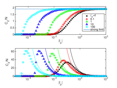
Figure 1: The contacts of $C_{2}$ and $C_{4}$ at the ground state of the model with particle number $N=4$. The symbols denote the numerical curves determined from equations (21), (23), and (24). Wheres the dashed lines are the strong coupling result from (62).

IV Correlation Function

In this section, we present a straightforward calculation of the contact $C_{2}$, and $C_{4}$ for weak interaction regime, i.e. $\left|l_{p}\right|\ll 1/2\pi n$ and $\xi_{p}<1/2\pi n$, where the particle number density $n=N/L$. Following the method used for calculating high order local and nonlocal correlation functions of 1D strong interaction Bose gas Nandani et al. (2016), we may directly calculate the correlation functions of the 1D p-wave Fermi gases up to the second order of $\left|l_{p}\right|$ .

IV.1 Weak Interaction

For weak interaction, i.e. $\left|l_{p}\right|\ll 1/2\pi n$ and $\xi_{p}<1/2\pi n$, the coefficients $a\left(P\right)$ in the wave function can be expanded up to the second order of $\left|l_{p}\right|$ with the following form

$$a\left(P\right)\approx\left(-1\right)^{P}\prod_{i<j=1}^{N}\left(1-\left|l_{p}\right|\textrm{i}\left(\lambda_{P_{i}}-\lambda_{P_{j}}\right)-\frac{1}{2}l_{p}^{2}\left(\lambda_{P_{i}}-\lambda_{P_{j}}\right)^{2}\left[1+2\textrm{i}\xi_{p}\left(\lambda_{P_{i}}-\lambda_{P_{j}}\right)\right]\right),$$ (26)

and as a result the wave function in the domain $\left\{0\leq z_{1}\leq\cdots\leq z_{N}\leq L\right\}$ for $z_{2}=z_{1}+\varepsilon$ has the new form

$$\psi\left(z_{1},\cdots,z_{N}\right)=\psi^{\left(1\right)}\left(z_{1},\cdots,z_{N}\right)\left|l_{p}\right|+\psi^{\left(2\right)}\left(z_{1},\cdots,z_{N}\right)l_{p}^{2},$$ (27)

in which the wave function to the first order and the second order of $\left|l_{p}\right|$ are given by

$$\psi^{\left(1\right)}\left(z_{1},\cdots,z_{N}\right)=\left(\partial_{z_{2}}-\partial_{z_{1}}\right)\psi^{\left(0\right)}\left(z_{1},\cdots,z_{N}\right),$$ (28)

$$\psi^{\left(2\right)}\left(z_{1},\cdots,z_{N}\right)=-\left[\xi_{p}\left(\partial_{z_{2}}-\partial_{z_{1}}\right)^{2}+\left(N-2\right)\left(\partial_{z_{2}}+\partial_{z_{1}}\right)+\sum_{i=3}^{N}\left(N+1-2i\right)\partial_{z_{i}}\right]\psi^{\left(1\right)}\left(z_{1},\cdots,z_{N}\right),$$ (29)

respectively. Here the zeroth order wave function $\psi^{\left(0\right)}$ has the form of a Slater determinant $\psi^{\left(0\right)}\left(z_{1},\cdots,z_{N}\right)=\sum_{P}\left(-1\right)^{P}e^{\mathrm{i}\sum_{j=1}^{N}\lambda_{P_{j}}z_{j}}$. Without loss of generality we shall assume that $\lambda_{1}<\lambda_{2}<\cdots<\lambda_{N}$. Using the wave function (27), we can show that up to the order of $\left|l_{p}\right|^{3}$, the numerator of the two body correlation function (20) for a positive infinitesimal $\varepsilon$ reads (for details, see calculation in Appendix A).

$$g_{2}\left(y_{1},y_{2};z_{1},z_{2}\right)=\left\{1-\left|l_{p}\right|\xi_{p}\left[\left(\partial_{y_{2}}-\partial_{y_{1}}\right)^{2}+\left(\partial_{z_{2}}-\partial_{z_{1}}\right)^{2}\right]\right\}g_{2}^{\left(2\right)}\left(y_{1},y_{2};z_{1},z_{2}\right).$$ (30)

Here the second order correlation function is defined as the following derivatives

$$g_{2}^{\left(2\right)}\left(y_{1},y_{2};z_{1},z_{2}\right)=l_{p}^{2}\left(\partial_{y_{2}}-\partial_{y_{1}}\right)\left(\partial_{z_{2}}-\partial_{z_{1}}\right)g_{2}^{\left(0\right)}\left(y_{1},y_{2};z_{1},z_{2}\right).$$ (31)

In the above calculation, we have omitted higher order of $|l_{p}|\xi_{p}$ terms. We define the zeroth order correlation function

$$g_{2}^{\left(0\right)}\left(y_{1},y_{2};z_{1},z_{2}\right)=\int_{0}^{L}dz_{3}\cdots\int_{0}^{L}dz_{N}\left[\psi^{\left(0\right)}\left(y_{1},y_{2},z_{3},\cdots,z_{N}\right)\right]^{*}\psi^{\left(0\right)}\left(z_{1},z_{2},z_{3},\cdots,z_{N}\right).$$ (32)

This zeroth order correlation function goes to zero when we set up the short distance limit $\varepsilon\rightarrow 0$ (due to the zeroth order wave function $\psi^{\left(0\right)}\left(z_{1},\cdots,z_{N}\right)$). However, its derivatives gives non-zero results when taking the limit $\varepsilon\to 0$.

From BA equations (6) with the weak interaction, we can obtain the solution $\lambda_{i}=\lambda_{i}^{F}\alpha$ for total momentum $\sum_{i}\lambda_{i}=0$, where $\lambda_{i}^{F}=2\pi J_{i}/L$, $\alpha=1-2\left|l_{p}\right|n$, and the $J_{i}$ are (half-)integers satisfying $J_{1}<J_{2}<...<J_{N}$. Under the scaling $z_{i}=z_{i}^{F}/\alpha$, the zeroth order wave function $\psi^{\left(0\right)}\left(z_{1},\cdots,z_{N}\right)$ is identical to the form for ideal Fermi gas $\psi^{F}\left(z_{1}^{F},\cdots,z_{N}^{F}\right)=\sum_{P}\left(-1\right)^{P}e^{\mathrm{i}\sum_{j=1}^{N}\lambda_{P_{j}}^{F}z_{j}^{F}}$. We also find the normalization condition Nandani et al. (2016)

$$\int_{0}^{L}dz_{1}\cdots\int_{0}^{L}dz_{N}\left|\psi\left(z_{1},\cdots,z_{N}\right)\right|^{2}=\alpha^{1-N}\int_{0}^{L}dz_{1}^{F}...\int_{0}^{L}dz_{N}^{F}\left|\psi^{F}\left(z_{1}^{F},\cdots,z_{N}^{F}\right)\right|^{2}.$$ (33)

Then the zeroth order correlation function with normalization factor has the following form

$$g_{2}^{\left(0\right)}\left(y_{1},y_{2};z_{1},z_{2}\right)=\alpha N\left(N-1\right)\frac{\int_{0}^{L}dz_{3}^{F}\cdots\int_{0}^{L}dz_{N}^{F}\left[\psi^{F}\left(y_{1}^{F},y_{2}^{F},z_{3}^{F},\cdots,z_{N}^{F}\right)\right]^{*}\psi^{F}\left(z_{1}^{F},z_{2}^{F},z_{3}^{F},\cdots,z_{N}^{F}\right)}{\int_{0}^{L}dz_{1}^{F}...\int_{0}^{L}dz_{N}^{F}\left|\psi^{F}\left(z_{1}^{F},\cdots,z_{N}^{F}\right)\right|^{2}}.$$ (34)

Since $\psi^{F}\left(z_{1}^{F},\cdots,z_{N}^{F}\right)$ is a Slater determinant, one can use Wick’s theorem Nandani et al. (2016)

$$g_{2}^{\left(0\right)}\left(y_{1},y_{2};z_{1},z_{2}\right)=\alpha\left[G\left(y_{1}^{F},z_{1}^{F}\right)G\left(y_{2}^{F},z_{2}^{F}\right)-G\left(y_{1}^{F},z_{2}^{F}\right)G\left(y_{2}^{F},z_{1}^{F}\right)\right],$$ (35)

where the single particle reduced density matrix of ideal fermions is given by $G\left(y,z\right)=\frac{1}{L}\sum_{i=1}^{N}\exp\left[-\textrm{i}\lambda_{i}^{F}\left(y-z\right)\right]$. Substituting the above formula into expression (31), then substituting (31) into equation (30) and after a lengthy calculation, we obtain the two body correlation function (for details, see calculation in Appendix A)

$$g_{2}\left(y_{1},y_{2};z_{1},z_{2}\right)=l_{p}^{2}\frac{1}{L^{2}}\sum_{i,j=1}^{N}\left[\alpha^{3}\left(\lambda_{i}^{F}-\lambda_{j}^{F}\right)^{2}+2\left|l_{p}\right|\alpha^{5}\xi_{p}\left(\lambda_{i}^{F}-\lambda_{j}^{F}\right)^{4}\right]X\left(\lambda_{i}^{F},\lambda_{j}^{F}\right),$$ (36)

where $X\left(\lambda_{i}^{F},\lambda_{j}^{F}\right)=\exp\left[-\textrm{i}\lambda_{i}^{F}\left(y_{1}^{F}-z_{1}^{F}\right)\right]\exp\left[-\textrm{i}\lambda_{j}^{F}\left(y_{2}^{F}-z_{2}^{F}\right)\right]+\exp\left[-\textrm{i}\lambda_{i}^{F}\left(y_{1}^{F}-z_{2}^{F}\right)\right]\exp\left[-\textrm{i}\lambda_{j}^{F}\left(y_{2}^{F}-z_{1}^{F}\right)\right]$. We will use this expression to calculate the p-wave contacts.

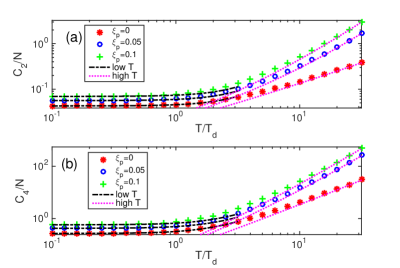
Figure 2: The Contacts for p-wave Fermi gas with weakly attractive interaction in the thermodynamic limit for $\left|l_{p}\right|=0.1$ and $n=1$. The marked-lines are exact results (40) and (41). The black dash-dot-lines are for low temperature limit (42) and (43). The magenta dot-lines are for high temperature limit (44) and (45). The Contacts $C_{2}$ and $C_{4}$ increase with both the temperature and the effective range.

IV.2 P-wave contacts

In the thermodynamic limit, we may use the Fermi distribution function to evaluate the p-wave contact through the relations given in (21)-(24). The modified Fermi distribution function with single particle energy $\left(\lambda^{F}\alpha\right)^{2}$ is given by

$$f\left(\lambda^{F}\right)=\frac{1}{1+\exp\left(\left[\left(\lambda^{F}\alpha\right)^{2}-A\right]/T\right)},$$ (37)

here $T$ and $A$ are the temperature and the effective chemical potential of the 1D Fermi gas respectively, and we have set Boltzmann constant $k_{B}=1$. It satisfies the normalization condition $\int_{-\infty}^{\infty}f\left(\lambda^{F}\right)\frac{L}{2\pi}d\lambda^{F}=N$, which include the first order modification of $\left|l_{p}\right|$ and is equivalent to the corresponding result from thermodynamical Bethe ansatz equations, see Appendix C. Notice that the density of states, i.e. the number of particles with fermionic momenta in the interval $(\lambda^{F},\lambda^{F}+d\lambda^{F})$, is $(L/2\pi)f\left(\lambda^{F}\right)d\lambda^{F}$, such that the summation in the two-body correlation function (36) becomes an integral in the following form

$$g_{2}\left(y_{1},y_{2};z_{1},z_{2}\right)=\frac{l_{p}^{2}}{4\pi^{2}}\int_{-\infty}^{\infty}d\lambda_{1}^{F}\int_{-\infty}^{\infty}d\lambda_{2}^{F}f\left(\lambda_{1}^{F}\right)f\left(\lambda_{2}^{F}\right)\left[\alpha^{3}\left(\lambda_{1}^{F}-\lambda_{2}^{F}\right)^{2}+2\left|l_{p}\right|\alpha^{5}\xi_{p}\left(\lambda_{1}^{F}-\lambda_{2}^{F}\right)^{4}\right]X\left(\lambda_{1}^{F},\lambda_{2}^{F}\right).$$ (38)

For our convenience in calculation, we make a change of variable $\lambda_{1,2}^{F}=2\pi nx_{1,2}$ and then we obtain

$$g_{2}\left(y_{1},y_{2};z_{1},z_{2}\right) = l_{p}^{2}4\pi^{2}n^{4}\int_{-\infty}^{\infty}dx_{1}\int_{-\infty}^{\infty}dx_{2}\mathscr{\mathcal{N}}\left(x_{1}\right)\mathcal{N}\left(x_{2}\right)\left[\alpha^{3}\left(x_{1}-x_{2}\right)^{2}+2\left|l_{p}\right|\alpha^{5}\xi_{p}\left(2\pi n\right)^{2}\left(x_{1}-x_{2}\right)^{4}\right]$$ (39)

$$\times X\left(2\pi nx_{1},2\pi nx_{2}\right),$$

where the function $\mathcal{N}\left(x\right)=f\left(2\pi nx\right)$ is subject to the normalization condition $\int_{-\infty}^{\infty}\mathcal{N}\left(x\right)dx=1$. Substituting the above formula into equations (21-24), we obtain explicitly the p-wave contacts in terms of the scattering length $\left|l_{p}\right|$ and the effective range $\xi_{p}$

$$C_{2} = 32\pi Nn^{3}l_{p}^{2}\left[\left(1-6\left|l_{p}\right|n\right)f_{2}+2\left|l_{p}\right|\xi_{p}\left(2\pi n\right)^{2}\left(f_{4}+3f_{2}^{2}\right)\right],$$ (40)

$$C_{4} = 32\pi^{3}Nn^{5}l_{p}^{2}\left[\left(1-10\left|l_{p}\right|n\right)\left(5f_{4}+3f_{2}^{2}\right)+2\left|l_{p}\right|\xi_{p}\left(2\pi n\right)^{2}\left(5f_{6}+27f_{2}f_{4}\right)\right],$$ (41)

with $f_{i}=\int_{-\infty}^{\infty}dx\mathcal{N}\left(x\right)x^{i}=\frac{1}{\left(2\pi n\alpha\right)^{i+1}}\int_{0}^{\infty}dy\frac{y^{\left(i-1\right)/2}}{1+e^{\left(y-A\right)/T}}$. We observe that that in the weak coupling regime the p-wave contacts $C_{2}$ and $C_{4}$ increase with both the scattering length $\left|l_{p}\right|$ and the effective range $\xi_{p}$. In addition we have checked that indeed $C_{3}=0$ for the ground state and equilibrium states.

At low temperature $T\ll T_{d}$, here $T_{d}=\frac{\hbar^{2}n^{2}}{2mk_{B}}$ is the degeneracy temperature, we can further calculate the contacts by the Sommerfeld expansion

$$C_{2}=\frac{8}{3}\pi Nn^{3}l_{p}^{2}\left[\left(1-6\left|l_{p}\right|n\right)+\left(1+2\left|l_{p}\right|n\right)\frac{1}{4\pi^{2}}\tau^{2}+\frac{16}{5}\left|l_{p}\right|\xi_{p}\left(\pi n\right)^{2}\left(1+\frac{5}{8\pi^{2}}\tau^{2}\right)\right],$$ (42)

$$C_{4}=\frac{8}{3}\pi^{3}Nn^{5}l_{p}^{2}\left[\left(1-10\left|l_{p}\right|n\right)+\left(1-2\left|l_{p}\right|n\right)\frac{3}{4\pi^{2}}\tau^{2}+\frac{132}{35}\left|l_{p}\right|\xi_{p}\left(\pi n\right)^{2}\left(1+\frac{14}{11\pi^{2}}\tau^{2}\right)\right],$$ (43)

with $\tau=T/T_{d}$, see Appendix B. This indicates a simple relationship between the leading terms of $C_{2}$ and $C_{4}$, i.e. $C_{4}=C_{2}\left(n\pi\right)^{2}$. In this weak coupling regime, the contact $C_{2}$ of the spinless p-wave Fermi gas behaves much likes the one of the Lieb-Liniger Bose gas with a strong repulsion Nandani et al. (2016). The contacts $C_{2}$ and $C_{4}$ increase smoothly as we increase the temperature. At relative high temperatures $T\gg T_{d}$, one can apply the Taylor series expansion with the distribution function $f_{i}$ under the condition $\exp\left(A/T\right)\ll 1$, and then one has

$$C_{2} = \frac{4}{\pi}\tau Nn^{3}l_{p}^{2}\left[\left(1-2\left|l_{p}\right|n\right)+\left(1-4\left|l_{p}\right|n\right)\frac{\sqrt{2\pi}}{2}\tau^{-1/2}+6\left|l_{p}\right|\xi_{p}n^{2}\tau\left(1+\frac{7\sqrt{2\pi}}{8}\tau^{-1/2}\right)\right],$$ (44)

$$C_{4} = \frac{9}{\pi}\tau^{2}Nn^{5}l_{p}^{2}\left[\left(1-2\left|l_{p}\right|n\right)+\left(1-4\left|l_{p}\right|n\right)\frac{19\sqrt{2\pi}}{24}\tau^{-1/2}+\frac{26}{3}\left|l_{p}\right|\xi_{p}n^{2}\tau\left(1+\frac{445\sqrt{2\pi}}{416}\tau^{-1/2}\right)\right].$$ (45)

In the above calculation, the weak interaction conditions require that $\left|l_{p}\right|/\Lambda\ll 1$, where the thermal de Broglie wavelength $\Lambda=\sqrt{\frac{4\pi}{k_{B}T}}$. Namely, we request $T\ll T_{d}/\left(l_{p}n\right)^{2}$ and $C_{2}/\left(Nn\right)\ll 1$. We show these low and high temperature behaviour of the contacts of the spinless Fermi gases with an attractive p-wave interaction in Figure 2, where a good agreement between the numerical result and the exact result which we have obtained here.

IV.3 Energy derivatives with respect to the scattering length

To related the $p$-wave contact defined using asymptotic behavior of the momentum distribution to other physical observables, let us consider how $C_{2}$ is related to the derivative of energy with respect to $l_{p}$. Since the sub-leading $C_{4}$ term involves two contacts $C_{4}^{r}$ and $C_{4}^{c}$, and only the former is related to energy derivative with respect to the effective range, we shall not discuss that adiabatic relation in this work. To that end, let us consider the $p$-wave pseudopotential of the following form Girardeau et al. (2004); Grosse et al. (2004)

$$V\left(z_{1},\cdots z_{N}\right)=-a_{p}^{1D}\sum_{i<j}\left(\frac{\partial}{\partial z_{i}}-\frac{\partial}{\partial z_{j}}\right)\delta\left(z_{i}-z_{j}\right)\left(\frac{\partial}{\partial z_{i}}-\frac{\partial}{\partial z_{j}}\right).$$ (46)

According to the Hellman-Feynman theorem, the two body correlation function is related to derivative of energy with respect to $a_{p}^{\textrm{1D}}$, i.e. $g_{2}\left(0,\varepsilon;0,\varepsilon\right)=\frac{\left(a_{p}^{\textrm{1D}}\right)^{2}}{2L}\frac{\partial E}{\partial a_{p}^{\textrm{1D}}}$. Combining the definition of contact $C_{2}$ with the effective scattering length $l_{p}=a_{p}^{\mathrm{1D}}/2$, we may verify that the following relationship holds: $C_{2}=\frac{1}{\pi}\frac{\partial E}{\partial\left(-a_{p}^{1D}\right)^{-1}}$. For a grand canonical ensemble, this relation can be rewritten as

$$C_{2}=\frac{L}{\pi}\left.\frac{\partial P}{\partial\left(a_{p}^{1D}\right)^{-1}}\right|_{\mu,T},$$ (47)

where the pressure $P$ at finite temperatures and arbitrary an interaction strength can be obtained by thermodynamical Bethe ansatz (TBA) equations for the model, see Appendix C. Then one can recover the two-body correlation function, and thereafter the Contact $C_{2}$ given in (42) and (44).

Here we firstly study the ground energy and its corresponding contact using the BA equations, then further analytically calculate the finite temperature contact using the TBA equations. For the ground state under condition $\left|l_{p}\right|\ll L$ and $\xi_{p}\ll L$, the BA equations (7) give a class of asymptotic solutions

$$\lambda_{i}=\lambda_{i}^{F}\left[1-2n\left|l_{p}\right|+(4n^{2}-2\xi_{p}(n\left(\lambda_{i}^{F}\right)^{2}+3E^{F}/L))l_{p}^{2}\right]$$ (48)

up to the second order of $\left|l_{p}\right|$, where $\lambda_{i}^{F}$ and $E^{F}$ are quasi-momentum and energy for 1D ideal Fermi gases, respectively. Consequently, we have the ground state energy

$$E=E^{F}\left[1-4n\left|l_{p}\right|+4(3n^{2}-\xi_{p}(n\sum_{i=1}^{N}\left(\lambda_{i}^{F}\right)^{4}/E^{F}+3E^{F}/L))l_{p}^{2}\right].$$ (49)

Taking derivative of the ground state energy with respect to 1D scattering length, we obtain the contact

$$C_{2}=\frac{1}{\pi}8nE^{F}l_{p}^{2}\left[1-6n\left|l_{p}\right|+2\xi_{p}\left|l_{p}\right|(\sum_{i=1}^{N}\left(\lambda_{i}^{F}\right)^{4}/E^{F}+3E^{F}/N))\right].$$ (50)

In the thermodynamics limit, the contact $C_{2}=\frac{8}{3}\pi n^{3}Nl_{p}^{2}\left(1-6n\left|l_{p}\right|+\frac{16}{5}\xi_{p}\left|l_{p}\right|\pi^{2}n^{2}\right)$ is consistent with expression given in (42) for the ground state.

In the following we consider the grand canonical ensemble in order to confirm the relation (47). For $l_{p}<0$, all solutions of the BA equations Eq. (6) are real. However, at finite temperatures, the eigenstates become degenerate. Following the approach to the thermodynamics of the 1D Bose gas introduced by C. N. Yang and C. P. Yang Yang and Yang (1969), here the Gibbs free energy $G=E-TS-\mu N$ of the spinless Fermi gases with an attractive p-wave interaction can be determined by a minimization the Gibbs energy, i.e. $\delta G$ with respect to the BA root densities. In the Gibbs free energy, $S$ denotes entropy and $\mu$ is the chemical potential. It follows that

$$\epsilon(\lambda)=\lambda^{2}-\mu-\frac{T}{2\pi}\int_{-\infty}^{\infty}K\left(k-\lambda\right)\mathrm{ln}\left\{1+\mathrm{exp}\left[-\epsilon\left(k\right)/T\right]\right\}dk,$$ (51)

where $\epsilon(\lambda)$ is the dressed energy characterizing the excitation energy. In the above equation, the kernel function $K(x)$ is given by

$$K(x)=\frac{2|l_{p}|(|l_{p}|\xi_{p}x^{2}+1)}{(|l_{p}|\xi_{p}x^{2}-1)^{2}+l_{p}^{2}x^{2}}.$$ (52)

The pressure $P$ can then be expressed as

$$P=\frac{T}{2\pi}\int_{-\infty}^{\infty}\mathrm{ln}\left\{1+\mathrm{exp}\left[-\epsilon\left(\lambda\right)/T\right]\right\}d\lambda.$$ (53)

This gives the equation of states, from which the particle density and the compressibility are determined by $n=\frac{\partial P}{\partial\mu}$ and $\kappa=\frac{\partial n}{\partial\mu}$, respectively.

In the weak interaction limit ($\left|l_{p}\right|\ll 1$), one can expand the kernel function $K(x)$ in powers of scattering length $\left|l_{p}\right|$. Up to the first few leading terms, the TBA equation (90) can be simplified as

$$\epsilon(\lambda)=B\lambda^{2}-A$$ (54)

where the effective chemical potential $A=\mu+2Q_{0}\left|l_{p}\right|+6\xi_{p}Q_{2}l_{p}^{2}$ with the notations $B=1-6\xi_{p}Q_{0}l_{p}^{2}$ and $Q_{j}=\frac{T}{2\pi}\int_{-\infty}^{\infty}k^{j}\mathrm{ln}\left\{1+\mathrm{exp}\left[-\frac{\epsilon\left(k\right)}{T}\right]\right\}dk$.

In the low temperature limit ($T\ll T_{d}$), the pressure $P$ up to the second order of $\left|l_{p}\right|$ reads

$$P=\frac{2}{3\pi}\mu^{3/2}\left\{1+2\frac{\sqrt{\mu}}{\pi}\left|l_{p}\right|+\left(\frac{14}{3}+\frac{16\pi}{5}\sqrt{\mu}\xi_{p}\right)\frac{\mu}{\pi^{2}}l_{p}^{2}+\frac{\pi^{2}}{8}\frac{T^{2}}{\mu^{2}}\left[1+\frac{4}{3}\frac{\sqrt{\mu}}{\pi}\left|l_{p}\right|+\left(\frac{10}{3}+\frac{48\pi}{5}\sqrt{\mu}\xi_{p}\right)\frac{\mu}{\pi^{2}}l_{p}^{2}\right]\right\}.$$ (55)

This gives an important indication of the deviation from the free fermions. From the formula (47), the Contact is calculated in a straightforward way

$$C_{2}=\frac{8Ll_{p}^{2}}{3\pi^{3}}\mu^{2}\left\{1+\left(\frac{14}{3}+\frac{16\pi}{5}\sqrt{\mu}\xi_{p}\right)\frac{\sqrt{\mu}}{\pi}\left|l_{p}\right|+\frac{\pi^{2}}{12}\frac{T^{2}}{\mu^{2}}\left[1+\left(5+\frac{72\pi}{5}\sqrt{\mu}\xi_{p}\right)\frac{\sqrt{\mu}}{\pi}\left|l_{p}\right|\right]\right\}.$$ (56)

In this expression, the chemical potential can be expressed in terms of the particle density

$$\mu=\pi^{2}n^{2}\left\{1-\frac{16}{3}n\left|l_{p}\right|+4n^{2}l_{p}^{2}\left(5-\frac{16\pi^{2}}{5}n\xi_{p}\right)+\frac{1}{12}\frac{T^{2}}{\pi^{2}n^{4}}\left[1-4n^{2}l_{p}^{2}\left(1+8\pi^{2}n\xi_{p}\right)\right]\right\}.$$ (57)

The above $p$-wave contact $C_{2}$ (56) is indeed consistent with expression (42), which was obtained from the many-body wave function. This confirms the universal relation (47). Furthermore the compressibility has the analytical form

$$\kappa=\frac{1}{2n\pi^{2}}\left(1+\frac{1}{12\pi^{2}}\frac{T^{2}}{n^{4}}\right)\left\{1+\left(8+\frac{2}{3\pi^{2}}\frac{T^{2}}{n^{4}}\right)n\left|l_{p}\right|+\left[24+\frac{22}{3\pi^{2}}\frac{T^{2}}{n^{4}}+\left(32\pi^{2}+4\frac{T^{2}}{n^{4}}\right)n\xi_{p}\right]n^{2}l_{p}^{2}\right\}.$$ (58)

Furthermore, for a relative high temperature regime, i.e. $T_{d}\ll T\ll T_{d}/\left(l_{p}n\right)^{2}$, up to the second order of $\left|l_{p}\right|$, the pressure is given by

$$P=\frac{1}{2}\frac{ZT^{3/2}}{\sqrt{\pi}}\left\{1-\frac{\sqrt{2}}{4}Z+\frac{Z\sqrt{T}}{\sqrt{\pi}}\left|l_{p}\right|\left(1-\frac{3\sqrt{2}}{4}Z\right)+\frac{3}{2\pi}ZTl_{p}^{2}\left[Z-\frac{4\sqrt{2}}{3}Z^{2}+2\sqrt{\pi T}\xi_{p}\left(1-\frac{9\sqrt{2}}{16}Z\right)\right]\right\},$$ (59)

here fugacity $Z=\exp\left(\mu/T\right)$. From the relation (47), the two-body correlation function is given explicitly

$$C_{2}=\frac{T^{2}Z^{2}l_{p}^{2}}{2\pi}\left\{1-\frac{3\sqrt{2}}{4}Z+3\sqrt{T/\pi}\left|l_{p}\right|\left[Z-\frac{4\sqrt{2}}{3}Z^{2}+2\sqrt{\pi T}\xi_{p}\left(1-\frac{9\sqrt{2}}{16}Z\right)\right]\right\}.$$ (60)

It is obvious that this result is consistent with expression (44) obtained from the many-body wave function (for details, see calculation in Appendix C). This alternative procedure provides a confirmation of the contact calculated by the many-body wave function in terms of the leading and sub-leading terms of the scattering length $\left|l_{p}\right|$, see Fig. 2.

IV.4 Strong Interaction Limit

The case $l_{p}\rightarrow-\infty$ is known as the Fermionic Tonks-Girardeau gas Bender et al. (2005); Girardeau and Minguzzi (2006) at the p-wave resonance. When, in addition, the effective range tends to zero, the wave function can be constructed from the noninteracting Bose gas with a sign function Bender et al. (2005); Girardeau and Minguzzi (2006). In the strong attractive coupling limit, i.e. $\left|l_{p}\right|\gg L+2N\xi_{p}$, the system has the similar solution of the quasi-momenta for the 1D weakly interacting Bose gas, see review Jiang et al. (2015). In this case, we assume that $\left|-\xi_{p}\lambda^{2}+1/\left|l_{p}\right|\right|\ll\left|\lambda\right|$ and find that the phase shift $\theta\left(\lambda\right)$ in the BA equations (6) is close to $\pm\pi$, and thus the quasi-momenta $\lambda_{i}$ are proportional to the square root of $1/\left|l_{p}\right|$ in the form $\lambda_{i}=\beta_{i}H\left(\xi_{p}\right)/\sqrt{\left|l_{p}\right|}$ with $i=1,\cdots,N$, in which the function $H\left(\xi_{p}\right)=\sqrt{2/\left(L+2N\xi_{p}\right)}$. Here $\left\{\beta_{i}\right\}$ with $N=1,\,2,\ldots,\,N$ are determined by the sets of equations $\beta_{i}=\sum_{j=1\left(j\neq i\right)}^{N}1/\left(\beta_{i}-\beta_{j}\right)$, which are equivalent to the roots of the Hermite polynomial of degree $N$. The summation of all squares of $\beta_{i}$ gives $\sum_{i}^{N}\beta_{i}^{2}=N\left(N-1\right)/2$, so that the energy of system is given by $E=N\left(N-1\right)/\left[\left(L+2N\xi_{p}\right)\left|l_{p}\right|\right]$. It is obvious that the energy decreases with an increase of the scattering length $\left|l_{p}\right|$ and the effective range $\xi_{p}$.

The coefficients in the wave function can be rewritten as $a\left(P\right)=\exp\left(\textrm{i}B\left(P\right)/\sqrt{\left|l_{p}\right|}\right)$ with $B\left(P\right)=\sum_{i<j}F\left(\xi_{p},\beta_{P_{i}}-\beta_{P_{j}}\right)$ and $F\left(\xi_{p},\beta\right)=\left(1-\xi_{p}H^{2}\left(\xi_{p}\right)\beta^{2}\right)/\left(H\left(\xi_{p}\right)\beta\right)$. The wave function in the domain $z_{1}\leq z_{2}\leq...\leq z_{N}$ is reduced into the following form

$$\psi\left(z_{1},z_{2},...,z_{N}\right)=N!-\frac{1}{2}\sum_{P}\left[B\left(P\right)+H\left(\xi_{p}\right)\sum_{j=1}^{N}\beta_{P_{j}}z_{j}\right]^{2}\frac{1}{\left|l_{p}\right|}+\mathcal{O}\left(\left|l_{p}\right|^{-3/2}\right).$$ (61)

By calculating the quasi-local correlation function (see Appendix D), one obtains the leading terms for $C_{2}$ and $C_{4}$ as following

$$C_{2}=\frac{2}{\pi}n\left(N-1\right),\qquad C_{4}=\frac{n}{\left|l_{p}\right|}\frac{4\left(N-1\right)^{2}}{\pi L\left(1+2n\xi_{p}\right)}.$$ (62)

From above expression, we see that the contact per particle $C_{2}/N$ is a finite value that depends only on the particle density in the thermodynamical limit. However, $C_{4}$ decreases with an increase of the scattering length $\left|l_{p}\right|$, and it goes to zero at the p-wave resonance $\left|l_{p}\right|\rightarrow\infty$. For $\xi_{p}=0$, $C_{2}$ still has the same result as (62) which can be obtained from the energy derivative with respect to $\left|l_{p}\right|^{-1}$ Bender et al. (2005); Girardeau and Minguzzi (2006); Sekino et al. (2018).

V Conclusion

In summary, using the exact man-body Bethe ansatz wave function, we have obtained the large-momentum tails of momentum distribution of a spinless Fermi gas interacting via $p$-wave scattering. We have found the leading and sub-leading coefficients of $1/p^{2}$ and $1/p^{4}$, i.e. the $p$-wave contacts, and give their analytic expressions in both weak and strong interaction limit. We show also by explicit calculation how the $p$-wave contacts are related to the short-distance behavior of the two-body correlation functions. In addition, we have obtained the energetics and contacts in both the low and high temperature limits via thermodynamic Bethe ansatz. Our results provide a deep insight into the nature of the p-wave contacts in one and higher dimensions.

Appendix A Correlation Function

In the domain $z_{1}\leq z_{2}\leq...\leq z_{N}$, the wave function has the following form

$$\psi\left(z_{1},\cdots,z_{N}\right)=\sum_{P}a\left(P\right)e^{\mathrm{i}\sum_{j=1}^{N}\lambda_{P_{j}}z_{j}}.$$ (63)

For weak interaction, the coefficients $a\left(P\right)$ in above wave function can be expanded up to the second order of $\left|l_{p}\right|$

$$a\left(P\right)\approx\left(-1\right)^{P}\prod_{i<j}\left(1-\left|l_{p}\right|\textrm{i}\left(\lambda_{P_{i}}-\lambda_{P_{j}}\right)-\frac{1}{2}l_{p}^{2}\left(\lambda_{P_{i}}-\lambda_{P_{j}}\right)^{2}\left[1+2\textrm{i}\xi_{p}\left(\lambda_{P_{i}}-\lambda_{P_{j}}\right)\right]\right).$$ (64)

When $z_{2}=z_{1}+\varepsilon$, the coefficients $a\left(P_{1}P_{2}P_{3}...P_{N}\right)$ and $a\left(P_{2}P_{1}P_{3}...P_{N}\right)$ share the same plane wave $e^{\mathrm{i}\left(\lambda_{P_{1}}+\lambda_{P_{2}}\right)z_{1}+\mathrm{i}\sum_{j=3}^{N}\lambda_{P_{j}}z_{j}}$, so we calculate the summation of them

$$a\left(P_{1}P_{2}P_{3}...P_{N}\right)+a\left(P_{2}P_{1}P_{3}...P_{N}\right)$$

$$\approx 2\left(-1\right)^{P}\left(\frac{\left|l_{p}\right|}{\textrm{i}}\lambda_{P_{12}}+\frac{l_{p}^{2}\xi_{p}}{\textrm{i}}\lambda_{P_{12}}^{3}\right)\prod_{i<j=3}\left(1+\frac{\left|l_{p}\right|}{\textrm{i}}\lambda_{P_{ij}}\right)$$

$$\approx 2\left(-1\right)^{P}\left(\frac{\left|l_{p}\right|}{\textrm{i}}\lambda_{P_{12}}+\frac{l_{p}^{2}\xi_{p}}{\textrm{i}}\lambda_{P_{12}}^{3}-l_{p}^{2}\lambda_{P_{12}}\sum_{i<j=3}\lambda_{P_{ij}}\right)$$

$$=2\left(-1\right)^{P}\lambda_{P_{12}}\left(\frac{\left|l_{p}\right|}{\textrm{i}}+l_{p}^{2}\left[\frac{\xi_{p}}{\textrm{i}}\lambda_{P_{12}}^{2}-\left(N-2\right)\left(\lambda_{P_{1}}+\lambda_{P_{2}}\right)-\sum_{i=3}^{N}\left(N+1-2i\right)\lambda_{P_{i}}\right]\right),$$ (65)

in which $\lambda_{P_{ij}}=\lambda_{P_{i}}-\lambda_{P_{j}}$ and $\sum_{i<j=3}\lambda_{P_{ij}}=\left(N-2\right)\left(\lambda_{P_{1}}+\lambda_{P_{2}}\right)+\sum_{i=3}^{N}\left(N+1-2i\right)\lambda_{P_{i}}$. And then the wave function for $z_{2}=z_{1}+\varepsilon$ can be rewritten as

$$\psi\left(z_{1},\cdots,z_{N}\right) \approx\sum_{P}\left(-1\right)^{P}\lambda_{P_{12}}\left(\frac{\left|l_{p}\right|}{\textrm{i}}+l_{p}^{2}\left[\frac{\xi_{p}}{\textrm{i}}\lambda_{P_{12}}^{2}-\left(N-2\right)\left(\lambda_{P_{1}}+\lambda_{P_{2}}\right)-\sum_{i=3}^{N}\left(N+1-2i\right)\lambda_{P_{i}}\right]\right)e^{\mathrm{i}\sum_{j=1}^{N}\lambda_{P_{j}}z_{j}}$$

$$=\psi^{\left(1\right)}\left(z_{1},\cdots,z_{N}\right)\left|l_{p}\right|+\psi^{\left(2\right)}\left(z_{1},\cdots,z_{N}\right)l_{p}^{2},$$ (66)

in which the wave function to the first order and the second order of $\left|l_{p}\right|$ are given by

$$\psi^{\left(1\right)}\left(z_{1},\cdots,z_{N}\right) =\sum_{P}\left(-1\right)^{P}\frac{\lambda_{P_{12}}}{\textrm{i}}e^{\mathrm{i}\sum_{j=1}^{N}\lambda_{P_{j}}z_{j}}$$

$$=\sum_{P}\left(-1\right)^{P}\left(\partial_{z_{2}}-\partial_{z_{1}}\right)e^{\mathrm{i}\sum_{j=1}^{N}\lambda_{P_{j}}z_{j}}$$

$$=\left(\partial_{z_{2}}-\partial_{z_{1}}\right)\psi^{\left(0\right)}\left(z_{1},\cdots,z_{N}\right),$$ (67)

$$\psi^{\left(2\right)}\left(z_{1},\cdots,z_{N}\right) =\sum_{P}\left(-1\right)^{P}\lambda_{P_{12}}\left[\frac{\xi_{p}}{\textrm{i}}\lambda_{P_{12}}^{2}-\left(N-2\right)\left(\lambda_{P_{1}}+\lambda_{P_{2}}\right)-\sum_{i=3}^{N}\left(N+1-2i\right)\lambda_{P_{i}}\right]e^{\mathrm{i}\sum_{j=1}^{N}\lambda_{P_{j}}z_{j}}$$

$$=\sum_{P}\textrm{i}\left(-1\right)^{P}\left(\partial_{z_{2}}-\partial_{z_{1}}\right)\left[\textrm{i}\xi_{p}\left(\partial_{z_{2}}-\partial_{z_{1}}\right)^{2}+\textrm{i}\left(N-2\right)\left(\partial_{z_{2}}+\partial_{z_{1}}\right)+\textrm{i}\sum_{i=3}^{N}\left(N+1-2i\right)\partial_{z_{i}}\right]e^{\mathrm{i}\sum_{j=1}^{N}\lambda_{P_{j}}z_{j}}$$

$$=-\left[\xi_{p}\left(\partial_{z_{2}}-\partial_{z_{1}}\right)^{2}+\left(N-2\right)\left(\partial_{z_{2}}+\partial_{z_{1}}\right)+\sum_{i=3}^{N}\left(N+1-2i\right)\partial_{z_{i}}\right]\psi^{\left(1\right)}\left(z_{1},\cdots,z_{N}\right),$$ (68)

with the zeroth order wave function $\psi^{\left(0\right)}\left(z_{1},\cdots,z_{N}\right)=\sum_{P}\left(-1\right)^{P}e^{\mathrm{i}\sum_{j=1}^{N}\lambda_{P_{j}}z_{j}}$.

The correlation function without normalization for infinitesimal $y_{1},y_{2};z_{1},z_{2}$ is calculated by above wave function

$$g_{2}\left(y_{1},y_{2};z_{1},z_{2}\right)$$

$$=\int_{0}^{L}dz_{3}\cdots\int_{0}^{L}dz_{N}\psi^{*}\left(y_{1},y_{2},z_{3},\cdots\right)\psi\left(z_{1},\cdots,z_{N}\right)$$

$$=\left(N-2\right)!\int_{0\leq z_{3}\leq\cdots\leq z_{N}\leq L}\psi^{*}\left(y_{1},y_{2},z_{3},\cdots\right)\psi\left(z_{1},\cdots,z_{N}\right)$$

$$\approx\left(N-2\right)!\rho^{\left(\Delta\right)}l_{p}^{2}-\left(N-2\right)!\left|l_{p}^{3}\right|\left[\xi_{p}\left[\left(\partial_{z_{2}}-\partial_{z_{1}}\right)^{2}+\left(\partial_{y_{2}}-\partial_{y_{1}}\right)^{2}\right]+\left(N-2\right)\left(\partial_{z_{2}}+\partial_{z_{1}}+\partial_{y_{2}}+\partial_{y_{1}}\right)\right]\rho^{\left(\Delta\right)}$$

$$-\left(N-2\right)!\left|l_{p}^{3}\right|\sum_{i=3}^{N}\left(N+1-2i\right)\int_{0}^{L}\partial_{z_{i}}\rho_{i}^{\left(\Delta\right)}\left(z_{i}\right)dz_{i}.$$ (69)

in which

$$\rho^{\left(\Delta\right)}\equiv\int_{0\leq z_{3}\leq\cdots\leq z_{N}\leq L}\psi^{\left(1\right)*}\left(y_{1},y_{2},z_{3},\cdots\right)\psi^{\left(1\right)}\left(z_{1},\cdots,z_{N}\right)dz_{3}\cdots dz_{N},$$ (70)

$$\rho_{l}^{\left(\Delta\right)}\left(z_{l}\right)\equiv\int_{0\leq z_{3}\leq\cdots\leq z_{N}\leq L}\psi^{\left(1\right)*}\left(y_{1},y_{2},z_{3},\cdots\right)\psi^{\left(1\right)}\left(z_{1},\cdots,z_{N}\right)dz_{3}\cdots dz_{l-1}dz_{l+1}\cdots dz_{N},$$ (71)

with $3\leq l\leq N$. For the first term in the correlation function, we define the following derivatives

$$g_{2}^{\left(2\right)}\left(y_{1},y_{2};z_{1},z_{2}\right) \equiv\left(N-2\right)!\rho^{\left(\Delta\right)}l_{p}^{2}$$

$$=l_{p}^{2}\left(\partial_{y_{2}}-\partial_{y_{1}}\right)\left(\partial_{z_{2}}-\partial_{z_{1}}\right)\left(N-2\right)!\int_{0\leq z_{3}\leq\cdots\leq z_{N}\leq L}\psi^{\left(0\right)*}\left(y_{1},y_{2},z_{3},\cdots\right)\psi^{\left(0\right)}\left(z_{1},\cdots,z_{N}\right)dz_{3}\cdots dz_{N}$$

$$=l_{p}^{2}\left(\partial_{y_{2}}-\partial_{y_{1}}\right)\left(\partial_{z_{2}}-\partial_{z_{1}}\right)g_{2}^{\left(0\right)}\left(y_{1},y_{2};z_{1},z_{2}\right)$$ (72)

with $g_{2}^{\left(0\right)}\left(y_{1},y_{2};z_{1},z_{2}\right)=(N-2)\int_{0}^{L}dz_{3}\cdots\int_{0}^{L}dz_{N}\left[\psi^{\left(0\right)}\left(y_{1},y_{2},z_{3},\cdots\right)\right]^{*}\psi^{\left(0\right)}\left(z_{1},\cdots,z_{N}\right)$. The last term in the correlation function can be proved to be zero with

$$\int_{0}^{L}\partial_{z_{i}}\rho_{i}^{\left(\Delta\right)}\left(z_{i}\right)dz_{i}=\rho_{i}^{\left(\Delta\right)}\left(L\right)-\rho_{i}^{\left(\Delta\right)}\left(0\right)=0.$$ (73)

At last, one can obtain the correlation function

$$g_{2}\left(y_{1},y_{2};z_{1},z_{2}\right)=\left\{1-\left|l_{p}\right|\xi_{p}\left[\left(\partial_{z_{2}}-\partial_{z_{1}}\right)^{2}+\left(\partial_{y_{2}}-\partial_{y_{1}}\right)^{2}\right]\right\}g_{2}^{\left(2\right)}\left(y_{1},y_{2};z_{1},z_{2}\right).$$ (74)

The Bethe ansatz equations (7) for weak atrractive interaction ($\left|l_{p}\right|\ll L$) exhibit the asymptotic solution $\lambda_{i}=\lambda_{i}^{F}\alpha$ for total momentum $\sum_{i=1}^{N}\lambda_{i}=0$, where $\lambda_{i}^{F}=2\pi J_{i}/L$, $\alpha=1-2\left|l_{p}\right|n$, and the $J_{i}$ are (half-)integers satisfying $J_{1}<J_{2}<...<J_{N}$. Under the scaling $z_{i}=z_{i}^{F}/\alpha$, the zeroth order correlation function is simplified to

$$g_{2}^{0}\left(y_{1},y_{2};z_{1},z_{2}\right)\approx\alpha^{2-N}\int_{0}^{L}\psi^{F}\left(y_{1}^{F},y_{2}^{F},...,z_{N}^{F}\right)\psi^{F}\left(z_{1}^{F},z_{2}^{F},...,z_{N}^{F}\right)dz_{3}^{F}...dz_{N}^{F}$$ (75)

with wave function of ideal Fermi gas $\psi^{F}\left(z_{1}^{F},z_{2}^{F},...,z_{N}^{F}\right)=\sum_{Q}\left(-1\right)^{Q}e^{\mathrm{i}\sum_{j=1}^{N}k_{Q_{j}}^{F}z_{j}^{F}}$. Meanwhile using the normalization factorNandani et al. (2016)

$$\int_{0}^{L}dz_{1}...\int_{0}^{L}dz_{N}\left|\Psi\left(z_{1},z_{2},...,z_{N}\right)\right|^{2} = \alpha^{1-N}\int_{0}^{L}dz_{1}...\int_{0}^{L}dz_{N}\left|\psi^{\left(0\right)}\left(z_{1},z_{2},...,z_{N}\right)\right|^{2}$$ (76)

$$\approx \alpha^{1-N}\int_{0}^{L}dz_{1}^{F}...\int_{0}^{L}dz_{N}^{F}\left|\psi^{F}\left(z_{1}^{F},...,z_{N}^{F}\right)\right|^{2},$$

the zeroth order correlation function with normalization factor has the following form

$$g_{2}^{0}\left(y_{1},y_{2};z_{1},z_{2}\right)=\alpha N\left(N-1\right)\frac{\int_{0}^{L}\psi^{F}\left(y_{1}^{F},y_{2}^{F},...,z_{N}^{F}\right)\psi^{F}\left(z_{1}^{F},z_{2}^{F},...,z_{N}^{F}\right)dz_{3}^{F}...dz_{N}^{F}}{\int_{0}^{L}dz_{1}^{F}...\int_{0}^{L}dz_{N}^{F}\left|\psi^{F}\left(z_{1}^{F},...,z_{N}^{F}\right)\right|^{2}}.$$ (77)

Since $\psi^{F}\left(z_{1}^{F},z_{2}^{F},...,z_{N}^{F}\right)$ is a Slater determinant, thus one can obtain the following result by the Wick’s theorem

$$g_{2}^{0}\left(y_{1},y_{2};z_{1},z_{2}\right)=\alpha\left[G\left(y_{1}^{F},z_{1}^{F}\right)G\left(y_{2}^{F},z_{2}^{F}\right)-G\left(y_{1}^{F},z_{2}^{F}\right)G\left(y_{2}^{F},z_{1}^{F}\right)\right],$$ (78)

where the single particle reduced density matrix of ideal fermions is given by $G\left(y,z\right)=\frac{1}{L}\sum_{i=1}^{N}\exp\left[-\textrm{i}\lambda_{i}^{F}\left(y-z\right)\right]$. By using the above result, the two-body correlation function has the following form

$$g_{2}^{\left(2\right)}\left(y_{1},y_{2};z_{1},z_{2}\right) =l_{p}^{2}\left(\partial_{y_{2}}-\partial_{y_{1}}\right)\left(\partial_{z_{2}}-\partial_{z_{1}}\right)g_{2}^{\left(0\right)}\left(y_{1},y_{2};z_{1},z_{2}\right)$$

$$=l_{p}^{2}\alpha^{3}\left(\partial_{y_{2}^{F}}-\partial_{y_{1}^{F}}\right)\left(\partial_{z_{2}^{F}}-\partial_{z_{1}^{F}}\right)\left[G\left(y_{1}^{F},z_{1}^{F}\right)G\left(y_{2}^{F},z_{2}^{F}\right)-G\left(y_{1}^{F},z_{2}^{F}\right)G\left(y_{2}^{F},z_{1}^{F}\right)\right]$$

$$=l_{p}^{2}\frac{1}{L^{2}}\sum_{i,j=1}^{N}\alpha^{3}\left(\lambda_{i}^{F}-\lambda_{j}^{F}\right)^{2}X\left(\lambda_{i}^{F},\lambda_{j}^{F}\right),$$ (79)

where $X\left(\lambda_{i}^{F},\lambda_{j}^{F}\right)=\exp\left[-\textrm{i}\lambda_{i}^{F}\left(y_{1}^{F}-z_{1}^{F}\right)\right]\exp\left[-\textrm{i}\lambda_{j}^{F}\left(y_{2}^{F}-z_{2}^{F}\right)\right]+\exp\left[-\textrm{i}\lambda_{i}^{F}\left(y_{1}^{F}-z_{2}^{F}\right)\right]\exp\left[-\textrm{i}\lambda_{j}^{F}\left(y_{2}^{F}-z_{1}^{F}\right)\right]$. Finally, we have the two-body correlation function (36) in the main text, namely

$$g_{2}\left(y_{1},y_{2};z_{1},z_{2}\right)=l_{p}^{2}\frac{1}{L^{2}}\sum_{i,j=1}^{N}\left[\alpha^{3}\left(\lambda_{i}^{F}-\lambda_{j}^{F}\right)^{2}+2\left|l_{p}\right|\alpha^{5}\xi_{p}\left(\lambda_{i}^{F}-\lambda_{j}^{F}\right)^{4}\right]X\left(\lambda_{i}^{F},\lambda_{j}^{F}\right).$$ (80)

Appendix B P-wave contacts: $C_{2}$ and $C_{4}$

For the low temperature, $A/T\gg 1$, according to Sommerfeld expansion, the function $f_{i}=\int_{-\infty}^{\infty}dx\mathcal{N}\left(x\right)x^{i}=\frac{1}{\left(2\pi n\alpha\right)^{i+1}}\int_{0}^{\infty}dy\frac{y^{\left(i-1\right)/2}}{1+e^{\left(y-A\right)/T}}$ is expanded with respect to the temperature

$$f_{i}=\frac{1}{\left(2\pi n\alpha\right)^{i+1}}\left[\frac{2}{i+1}A^{\left(i+1\right)/2}+\frac{\pi^{2}\left(i-1\right)}{12}T^{2}A^{\left(i-3\right)/2}+...\right].$$ (81)

From the normalization condition $f_{0}=1$, the effective chemical potential $A$ can be solved by iteration method

$$A\approx\left(\pi n\alpha\right)^{2}\left(1+\frac{1}{12\pi^{2}}\frac{\tau^{2}}{\alpha^{4}}\right)$$ (82)

with $\tau=T/n^{2}$. And put the effective chemical potential into $f_{i}$, $f_{i}$ is expressed with $\tau$ and $\alpha$

$$f_{i}=\frac{1}{\left(i+1\right)2^{i}}\left[1+\frac{i\left(i+1\right)}{24\pi^{2}}\frac{\tau^{2}}{\alpha^{4}}+...\right]$$ (83)

and then one obtain the contact $C_{2}$ and $C_{4}$

$$C_{2}=\frac{8}{3}\left|l_{p}\right|^{2}\pi n^{3}N\left[\left(1-6\left|l_{p}\right|n\right)+\left(1+2\left|l_{p}\right|n\right)\frac{1}{4\pi^{2}}\tau^{2}+\frac{16}{5}\left|l_{p}\right|\xi_{p}\left(\pi n\right)^{2}\left(1+\frac{5}{8\pi^{2}}\tau^{2}\right)\right],$$ (84)

$$C_{4}=\frac{8}{3}\left|l_{p}\right|^{2}\pi^{3}n^{5}N\left[\left(1-10\left|l_{p}\right|n\right)+\left(1-2\left|l_{p}\right|n\right)\frac{3}{4\pi^{2}}\tau^{2}+\frac{132}{35}\left|l_{p}\right|\xi_{p}\left(\pi n\right)^{2}\left(1+\frac{14}{11\pi^{2}}\tau^{2}\right)\right].$$ (85)

For the relative high temperature which requires effective fugacity $Z_{A}\equiv\exp\left(A/T\right)\ll 1$, the integral $f_{i}$ is expanded by effective fugacity

$$f_{i} \approx\frac{1}{\left(2\pi n\alpha\right)^{i+1}}\int_{0}^{\infty}dyy^{\left(i-1\right)/2}Z_{A}e^{-y/T}\left(1-Z_{A}e^{-y/T}\right)$$

$$=\frac{T^{\left(i+1\right)/2}}{\left(2\pi n\alpha\right)^{i+1}}\Gamma\left(\frac{i+1}{2}\right)Z_{A}\left(1-2^{-\left(i+1\right)/2}Z_{A}\right).$$ (86)

From the normalization condition $f_{0}=1$, the effective fugacity can be solved by iteration method

$$Z_{A}\approx\frac{2\sqrt{\pi}\alpha}{\tau^{1/2}}\left(1+\frac{\sqrt{2\pi}\alpha}{\tau^{1/2}}\right),$$ (87)

and then one obtain the contact $C_{2}$ and $C_{4}$

$$C_{2}=\frac{4}{\pi}l_{p}^{2}Nn^{3}\tau\left[\left(1-2\left|l_{p}\right|n\right)+\left(1-4\left|l_{p}\right|n\right)\frac{\sqrt{2\pi}}{2}\tau^{-1/2}+6\left|l_{p}\right|\xi_{p}T\left(1+\frac{7\sqrt{2\pi}}{8}\tau^{-1/2}\right)\right],$$ (88)

$$C_{4}=\frac{9}{\pi}l_{p}^{2}Nn^{3}\tau^{2}\left[\left(1-2\left|l_{p}\right|n\right)+\left(1-4\left|l_{p}\right|n\right)\frac{19\sqrt{2\pi}}{24}\tau^{-1/2}+\frac{26}{3}\left|l_{p}\right|\xi_{p}T\left(1+\frac{445\sqrt{2\pi}}{416}\tau^{-1/2}\right)\right].$$ (89)

Appendix C The thermodynamic Bethe Ansatz equations

The thermodynamics Bethe Ansatz equation for p-wave fermions in one dimension can be written as

$$\epsilon(\lambda)=\frac{\hbar^{2}\lambda^{2}}{2m}-\mu-\frac{T}{2\pi}\int_{-\infty}^{\infty}K\left(k-\lambda\right)\mathrm{ln}\left\{1+\mathrm{exp}\left[-\epsilon\left(k\right)/T\right]\right\}dk$$ (90)

with $K(x)=\frac{2|l_{p}|(|l_{p}|\xi_{p}x^{2}+1)}{(|l_{p}|\xi_{p}x^{2}-1)^{2}+l_{p}^{2}x^{2}}$. The pressure is defined as

$$P=\frac{T}{2\pi}\int_{-\infty}^{\infty}\mathrm{ln}\left\{1+\mathrm{exp}\left[-\epsilon\left(\lambda\right)/T\right]\right\}d\lambda.$$ (91)

The grand canonical potential, the particle density per length and the contact are given by $\Omega=-PL$, $n=\frac{\partial P}{\partial\mu}$ and $C_{2}=\frac{2L}{\pi}l_{p}^{2}\frac{\partial P}{\partial|l_{p}|}$.

For weak interaction, $\left|l_{p}\right|<1/n$, the kernel in the integral function of equation (90)is expanded up to the second order of $\left|l_{p}\right|$

$$K(k-\lambda)\approx 2\left|l_{p}\right|+6\xi_{p}\left|l_{p}\right|^{2}\lambda^{2}+12\xi_{p}\left|l_{p}\right|^{2}\lambda k+6\xi_{p}\left|l_{p}\right|^{2}k^{2},$$ (92)

and then TBA equation is simplified as

$$\epsilon\left(\lambda\right)=B\lambda^{2}-A$$ (93)

with the effective chemical potential $A=\mu+2\left|l_{p}\right|Q_{0}+6Q_{2}\xi_{p}\left|l_{p}\right|^{2}$ with the notations $B=1-6Q_{0}\xi_{p}\left|l_{p}\right|^{2}$ and $Q_{j}=\frac{T}{2\pi}\int_{-\infty}^{\infty}k^{j}\mathrm{ln}\left\{1+\mathrm{exp}\left[-\frac{\epsilon\left(k\right)}{T}\right]\right\}dk$. Using integral by part, $Q_{j}$ can be expressed by polylogarithm

$$Q_{j}=-\left(\frac{T}{B}\right)^{\frac{j+1}{2}}\frac{T}{\pi\left(j+1\right)}\Gamma\left(\frac{j+3}{2}\right)\mathrm{Li}_{\frac{j+3}{2}}\left(-\mathrm{e}^{A/T}\right),$$ (94)

and using the properties of polylogarithm $\textrm{Li}_{i}\left(-\mathrm{e}^{A/T}\right)$, one obtain Pressure, particle density and contact with the following forms

$$P=-\frac{T^{3/2}}{2\sqrt{\pi}}\mathrm{Li}_{\frac{3}{2}}\left(-\mathrm{e}^{A/T}\right)\left(1-\frac{3T^{3/2}}{2\sqrt{\pi}}\mathrm{Li}_{\frac{3}{2}}\left(-\mathrm{e}^{A/T}\right)\xi_{p}\left|l_{p}\right|^{2}\right),$$ (95)

$$n=-\frac{T^{1/2}}{2\sqrt{\pi}}\mathrm{Li}_{\frac{1}{2}}\left(-\mathrm{e}^{A/T}\right)\left(1+2\left|l_{p}\right|n\right),$$ (96)

$$C_{2}=\frac{2L}{\pi}l_{p}^{2}n\left[2P-\left(\frac{3T^{5/2}}{\sqrt{\pi}}\mathrm{Li}_{\frac{5}{2}}\left(-\mathrm{e}^{A/T}\right)-\frac{6P^{2}}{n}\right)\xi_{p}\left|l_{p}\right|\right],$$ (97)

in which the expression of particle density is equivalent to previous normalization condition of modified Fermi-Dirac distribution function, and contact $C_{2}$ is also consistent with previous result from many-body wave function.

In the low temperature limit($T\ll T_{d}$), according to Sommerfeld expansion, $Q_{j}$ is expanded with respect to temperature

$$Q_{j}\approx\left(\frac{1}{B}\right)^{\frac{j+1}{2}}\frac{1}{\pi\left(j+1\right)}\left[\frac{2}{j+3}A^{\left(j+3\right)/2}+\frac{j+1}{2}\frac{\pi^{2}}{6}T^{2}A^{\left(j-1\right)/2}\right].$$ (98)

When the iteration method is applied, the pressure is rewritten as

$$P=\frac{2}{3\pi}\mu^{3/2}\left\{1+2\frac{\sqrt{\mu}}{\pi}\left|l_{p}\right|+\left(\frac{14}{3}+\frac{16\pi}{5}\sqrt{\mu}\xi_{p}\right)\frac{\mu}{\pi^{2}}l_{p}^{2}+\frac{\pi^{2}}{8}\frac{T^{2}}{\mu^{2}}\left[1+\frac{4}{3}\frac{\sqrt{\mu}}{\pi}\left|l_{p}\right|+\left(\frac{10}{3}+\frac{48\pi}{5}\sqrt{\mu}\xi_{p}\right)\frac{\mu}{\pi^{2}}l_{p}^{2}\right]\right\}.$$ (99)

According to formula $C_{2}=\frac{2L}{\pi}l_{p}^{2}\frac{\partial P}{\partial|l_{p}|}$, the contact is

$$C_{2}=\frac{8Ll_{p}^{2}}{3\pi^{3}}\mu^{2}\left\{1+\left(\frac{14}{3}+\frac{16\pi}{5}\sqrt{\mu}\xi_{p}\right)\frac{\sqrt{\mu}}{\pi}\left|l_{p}\right|+\frac{\pi^{2}}{12}\frac{T^{2}}{\mu^{2}}\left[1+\left(5+\frac{72\pi}{5}\sqrt{\mu}\xi_{p}\right)\frac{\sqrt{\mu}}{\pi}\left|l_{p}\right|\right]\right\},$$ (100)

in which chemical potential can be expressed by particle density with the form

$$\mu=\pi^{2}n^{2}\left[1-\frac{16}{3}n\left|l_{p}\right|+\frac{1}{12}\frac{T^{2}}{\pi^{2}n^{4}}\right].$$ (101)

At last one obtain the contact

$$C_{2}=\frac{8}{3}\pi l_{p}^{2}n^{3}N\left[\left(1-6|l_{p}|n\right)+\frac{1}{4}\frac{T^{2}}{\pi^{2}n^{4}}\left(1+2|l_{p}|n\right)+\frac{16}{5}n^{2}\pi^{2}\xi_{p}\left|l_{p}\right|\left(1+\frac{5}{8}\frac{T^{2}}{\pi^{2}n^{4}}\right)\right]$$ (102)

This result is consistent with that from many-body wave function.

For the relative high temperature, the fugacity $Z=\mathrm{e}^{\mu/T}\ll 1$, $Q_{j}$ can be expanded by fugacity

$$Q_{j}=\left(\frac{T}{B}\right)^{\frac{j+1}{2}}\frac{T}{\pi\left(j+1\right)}\Gamma\left(\frac{j+3}{2}\right)\mathrm{e}^{A/T}\left[1-2^{-\left(j+3\right)/2}\mathrm{e}^{A/T}+\mathrm{e}^{2A/T}3^{-\left(j+3\right)/2}-\mathrm{e}^{3A/T}4^{-\left(j+3\right)/2}\right].$$ (103)

When the iteration method is applied, the pressure is rewritten as

$$P=\frac{1}{2}\frac{ZT^{3/2}}{\sqrt{\pi}}\left[1-\frac{\sqrt{2}}{4}Z+\frac{Z\sqrt{T}}{\sqrt{\pi}}\left|l_{p}\right|\left(1-\frac{3\sqrt{2}}{4}Z\right)+\frac{3}{2}\frac{Z^{2}T}{\text{$\pi$}}l_{p}^{2}\left(1-\frac{4\sqrt{2}}{3}Z\right)+\frac{3ZT^{3/2}}{\sqrt{\text{$\pi$}}}l_{p}^{2}\xi_{p}\left(1-\frac{9\sqrt{2}}{16}Z\right)\right].$$ (104)

According to formula $C_{2}=\frac{2L}{\pi}l_{p}^{2}\frac{\partial P}{\partial|l_{p}|}$, the contact is

$$C_{2}=\frac{Ll_{p}^{2}Z^{2}T^{2}}{\pi^{2}}\left\{1-\frac{3}{4}\sqrt{2}Z+\left(1-\frac{4\sqrt{2}}{3}Z\right)\frac{3Z\sqrt{T}}{\sqrt{\pi}}|l_{p}|+6|l_{p}|\xi_{p}T\left(1-\frac{9}{16}\sqrt{2}Z\right)\right\},$$ (105)

in which fugacity can be expressed in particle density

$$Z=\frac{2\sqrt{\pi}n}{\sqrt{T}}\left(1+\frac{\sqrt{2\pi}n}{\sqrt{T}}\right)-\left(1+\frac{7\sqrt{2\pi}n}{4\sqrt{T}}\right)\frac{8\sqrt{\pi}n}{\sqrt{T}}|l_{p}|n.$$ (106)

At last, one obtain contact

$$C_{2}=\frac{4l_{p}^{2}TnN}{\pi}\left[1-2n|l_{p}|+\left(1-4n|l_{p}|\right)\frac{\sqrt{2\pi}}{2}\frac{n}{\sqrt{T}}+6|l_{p}|\xi_{p}T\left(1+\frac{7\sqrt{2\pi}}{8}\frac{n}{\sqrt{T}}\right)\right],$$ (107)

which is also consistent with that from many-body wave function.

Appendix D Strong coupling limit

The energy of system composed of $N$ spinless fermions can be expressed as $E=\sum_{i}^{N}\lambda_{i}^{2}$, and quasi-momentum $\lambda_{i}$ satisfy BA equation for real $\lambda_{i}$,

$$\lambda_{i}L=2\pi n_{i}-\sum_{j=1}^{N}\theta\left(\lambda_{i}-\lambda_{j}\right).$$ (108)

Here phase shift $\theta\left(\lambda\right)$ is a monotonic antisymmetric function defined by

$$\theta\left(\lambda\right)=2\arg\left(\textrm{i}\lambda-\xi_{p}\lambda^{2}+1/\left|l_{p}\right|\right)$$ (109)

and $n_{i}=i-\left(N+1\right)/2$ for ground state. In the strong attractive limit $\left|l_{p}\right|\gg 1/L$, and we assume that $\left|-\xi_{p}\lambda^{2}+1/\left|l_{p}\right|\right|\ll\left|\lambda\right|$, and then phase shift is approach to $\pm\pi$ with $\left(\lambda\right)\approx\pi\lambda/\left|\lambda\right|-2\left(\frac{x}{\lambda}-\xi_{p}\lambda\right)$ and $x\equiv 1/\left|l_{p}\right|$. And then BA equation becomes new form

$$\lambda_{i}L=\sum_{j=1\left(j\neq i\right)}^{N}\left[\frac{2x}{\lambda_{i}-\lambda_{j}}-2\xi_{p}\left(\lambda_{i}-\lambda_{j}\right)\right]$$ (110)

For the ground state, the total momentum is zero, which means $\sum_{j}\lambda_{j}=0$, so BA equation can be simplified as the new form

$$\left(L+2N\xi_{p}\right)\lambda_{i}=\sum_{j=1\left(j\neq i\right)}^{N}\frac{2x}{\lambda_{i}-\lambda_{j}}$$ (111)

The solution of above equation has the following form$\lambda_{i}=\sqrt{\frac{2x}{L+2N\xi_{p}}}\beta_{i}$, with constant $\beta_{i}$ which is determined by a set of equations $\beta_{i}=\sum_{j=1\left(j\neq i\right)}^{N}\frac{1}{\beta_{i}-\beta_{j}}$. The previous assumation $\left|-\xi_{p}\lambda^{2}+1/\left|l_{p}\right|\right|\ll\left|\lambda\right|$ requires that $\left|l_{p}\right|\gg L+2N\xi_{p}$, which is strong coupling condition for above solution. With above solution, the energy of system is

$$E=\frac{2/\left|l_{p}\right|}{L+2N\xi_{p}}\sum_{i}\beta_{i}^{2}=\frac{N\left(N-1\right)/\left|l_{p}\right|}{L+2N\xi_{p}}.$$ (112)

The coefficients in the wavefunction can be written as

$$a\left(P\right) = \left(-1\right)^{P}\prod_{i<j}\left(\exp\left(-\textrm{i}\theta\left(\lambda_{P_{i}}-\lambda_{P_{j}}\right)\right)\right)^{1/2}$$ (113)

$$= \exp\left(\textrm{i}\frac{\pi}{2}\left(1-\left(-1\right)^{P}\right)-\frac{\textrm{i}}{2}\sum_{i<j}\theta\left(\lambda_{P_{i}}-\lambda_{P_{j}}\right)\right).$$

In the strong attractive interaction limit, $\lambda_{i}=\frac{H\left(\xi_{p}\right)}{\sqrt{\left|l_{p}\right|}}\beta_{i}$ with $H\left(\xi_{p}\right)=\sqrt{\frac{2}{L+2N\xi_{p}}}$ , and phase shift $\theta\left(\lambda\right)\approx\frac{\lambda}{\left|\lambda\right|}\pi-2F\left(\xi_{p},\beta\right)\frac{1}{\sqrt{\left|l_{p}\right|}}$, with $F\left(\xi_{p},\beta\right)=\frac{1}{\sqrt{\frac{2}{L+2N\xi_{p}}}\beta}\left(1-\frac{2\xi_{p}}{L+2N\xi_{p}}\beta^{2}\right)$, and $F\left(\xi_{p},-\beta\right)=-F\left(\xi_{p},\beta\right)$. The coefficients has the following form

$$a\left(P\right)=\exp\left(\frac{\textrm{i}}{\sqrt{\left|l_{p}\right|}}B\left(P\right)\right)$$ (114)

with $B\left(P\right)=\sum_{i<j}F\left(\xi_{p},\beta_{P_{i}}-\beta_{P_{j}}\right)$. The wavefunction in the domain $z_{1}\leq z_{2}\leq...\leq z_{N}$ can be simplified as

$$\psi\left(z_{1},z_{2},...,z_{N}\right) = \sum_{P}\exp\left(\frac{\textrm{i}}{\sqrt{\left|l_{p}\right|}}B\left(P\right)\right)\exp\left(\frac{\mathrm{i}}{\sqrt{\left|l_{p}\right|}}H\left(\xi_{p}\right)\sum_{j=1}^{N}\beta_{P_{j}}z_{j}\right)$$ (115)

$$\approx N!-\frac{Y\left(z_{1},z_{2},...,z_{N},\xi_{p}\right)}{\left|l_{p}\right|}+\cdots$$

with $Y=\frac{1}{2}\sum_{P}\left[B\left(P\right)+H\left(\xi_{p}\right)\sum_{j=1}^{N}\beta_{P_{j}}z_{j}\right]^{2}$. The correlation function can be written as

$$g_{2}(y_{1},y_{2};z_{1},z_{2})$$

$$=\frac{N\left(N-1\right)\int_{0}^{L}dz_{3}...\int_{0}^{L}dz_{N}\psi^{*}\left(y_{1},y_{2},z_{3},...\right)\psi\left(z_{1},z_{2},z_{3},...\right)}{\int_{0}^{L}dz_{1}...\int_{0}^{L}dz_{N}\left|\Psi\left(z_{1},z_{2},...,z_{N}\right)\right|^{2}}$$

$$\approx\frac{N\left(N-1\right)\left[\left(N-2\right)!\right]N!}{\left(N!\right)^{2}L^{N}}\int_{0\leq z_{3}\leq...\leq z_{N}\leq L}dz_{3}...dz_{N}\left[N!-\frac{Y\left(y_{1},y_{2},z_{3},...,z_{N},\xi_{p}\right)}{\left|l_{p}\right|}-\frac{Y\left(z_{1},z_{2},...,z_{N},\xi_{p}\right)}{\left|l_{p}\right|}\right],$$ (116)

in which we suppose that $y_{1},y_{2},z_{1},z_{2}$ is close to zero. The leading term of contact $C_{2}$, $C_{4}^{r}$, $C_{4}^{c}$ and $C_{4}$ have the following results

$$C_{2} =\frac{2L}{\pi}g_{2}\left(0,\varepsilon;0,\varepsilon\right)$$

$$\approx\frac{2L}{\pi}\frac{N\left(N-1\right)\left(N!\right)^{2}L^{N-2}}{\left(N!\right)^{2}L^{N}}$$

$$=\frac{2}{\pi}\frac{N\left(N-1\right)}{L}.$$ (117)

$$C_{4}^{r} =-\frac{L}{\pi}\left[\textrm{Re}\left(\partial_{z_{2}}-\partial_{z_{1}}\right)^{2}g_{2}\left(y_{2}-\varepsilon,y_{2};z_{1},z_{2}\right)\right]_{y_{2}=z_{2}=z_{1}+\varepsilon}$$

$$\approx-\frac{L}{\pi}\frac{\frac{-1}{\left|l_{p}\right|}\left(N!\right)^{2}L^{N-2}\frac{2N}{L+2N\xi_{p}}N\left(N-1\right)}{\left(N!\right)^{2}L^{N}}$$

$$=\frac{1}{\pi}\frac{1}{\left|l_{p}\right|}\frac{2nN\left(N-1\right)}{L+2N\xi_{p}},$$ (118)

$$C_{4}^{c} =\frac{L}{2\pi}\left[\partial_{y_{2}}\partial_{z_{2}}g_{2}\left(y_{2}-\varepsilon,y_{2};z_{2}-\varepsilon,z_{2}\right)-2\textrm{Re}\partial_{z_{2}}^{2}g_{2}\left(y_{2}-\varepsilon,y_{2};z_{2}-\varepsilon,z_{2}\right)\right]_{y_{2}=z_{2}}$$

$$\approx 0+N^{2}\left(N-1\right)\frac{L}{2\pi N}\left(-2\right)\frac{-1}{\left|l_{p}\right|}\left(N!\right)^{2}L^{N-2}\frac{2}{L+2N\xi_{p}}\left(N-2\right)/\left[\left(N!\right)^{2}L^{N}\right]$$

$$=\frac{1}{\left|l_{p}\right|}\frac{2N\left(N-1\right)\left(N-2\right)}{\pi L\left(L+2N\xi_{p}\right)},$$ (119)

$$C_{4}=C_{4}^{c}+C_{4}^{r}=\frac{1}{\left|l_{p}\right|}\frac{4N\left(N-1\right)^{2}}{\pi L\left(L+2N\xi_{p}\right)}.$$ (120)

References

• Olshanii (1998) M. Olshanii, Phys. Rev. Lett. 81, 938 (1998).
• Bergeman et al. (2003) T. Bergeman, M. G. Moore, and M. Olshanii, Phys. Rev. Lett. 91, 163201 (2003).
• Paredes et al. (2004) B. Paredes, A. Widera, V. Murg, O. Mandel, S. Fölling, I. Cirac, G. V. Shlyapnikov, T. W. Hänsch, and I. Bloch, Nature 429, 277 (2004).
• Kinoshita (2004) T. Kinoshita, Science 305, 1125 (2004).
• Cazalilla et al. (2011) M. A. Cazalilla, R. Citro, T. Giamarchi, E. Orignac, and M. Rigol, Rev. Mod. Phys. 83, 1405 (2011).
• Guan et al. (2013) X.-W. Guan, M. T. Batchelor, and C. Lee, Rev. Mod. Phys. 85, 1633 (2013).
• Girardeau (1960) M. Girardeau, Journal of Mathematical Physics 1, 516 (1960).
• Giamarchi (2004) T. Giamarchi, (Oxford University Press, Oxford, 2004) (2004).
• Korepin et al. (1993) V. E. Korepin, N. M. Bogoliubov, and A. G. Izergin, (Cambridge: Cambridge University Press) (1993).
• Takahashi (1999) M. Takahashi, (Cambridge: Cambridge University Press) (1999).
• Essler et al. (2005) F. H. L. Essler, H. Frahm, G. F, K. A, and K. V. E, (Cambridge: Cambridge University Press) (2005).
• Sutherland (2004) B. Sutherland, (Singapore: World Scientific) (2004).
• Lieb and Liniger (1963) E. H. Lieb and W. Liniger, Phys. Rev. 130, 1605 (1963).
• Yang (1967) C. N. Yang, Phys. Rev. Lett. 19, 1312 (1967).
• Jiang et al. (2015) Y.-Z. Jiang, Y.-Y. Chen, and X.-W. Guan, Chin. Phys. B. 24, 050311 (2015).
• Haller et al. (2009) E. Haller, M. Gustavsson, M. J. Mark, J. G. Danzl, R. Hart, G. Pupillo, and H.-C. Nagerl, Science 325, 1224 (2009).
• Yang et al. (2017) B. Yang, Y.-Y. Chen, Y.-G. Zheng, H. Sun, H.-N. Dai, X.-W. Guan, Z.-S. Yuan, and J.-W. Pan, Phys. Rev. Lett. 119, 165701 (2017).
• Kinoshita et al. (2006) T. Kinoshita, T. Wenger, and D. S. Weiss, Nature 440, 900 (2006).
• Hofferberth et al. (2007) S. Hofferberth, I. Lesanovsky, B. Fischer, T. Schumm, and J. Schmiedmayer, Nature 449, 324 (2007).
• Guan et al. (2007) X.-W. Guan, M. T. Batchelor, and M. Takahashi, Phys. Rev. A 76, 043617 (2007).
• Deuretzbacher et al. (2014) F. Deuretzbacher, D. Becker, J. Bjerlin, S. M. Reimann, and L. Santos, Phys. Rev. A 90, 013611 (2014).
• Murmann et al. (2015) S. Murmann, F. Deuretzbacher, G. Zürn, J. Bjerlin, S. M. Reimann, L. Santos, T. Lompe, and S. Jochim, Phys. Rev. Lett. 115, 215301 (2015).
• Levinsen et al. (2015) J. Levinsen, P. Massignan, G. M. Bruun, and M. M. Parish, Science Advances 1, e1500197 (2015).
• Yang et al. (2015) L. Yang, L. Guan, and H. Pu, Phys. Rev. A 91, 043634 (2015).
• Hu et al. (2016) H. Hu, L. Pan, and S. Chen, Phys. Rev. A 93, 033636 (2016).
• Liu et al. (2017) Y. Liu, S. Chen, and Y. Zhang, Phys. Rev. A 95, 043628 (2017).
• Pan et al. (2017) L. Pan, Y. Liu, H. Hu, Y. Zhang, and S. Chen, Phys. Rev. B 96, 075149 (2017).
• Tan (2008a) S. Tan, Annals of Physics 323, 2952 (2008a).
• Tan (2008b) S. Tan, Annals of Physics 323, 2987 (2008b).
• Tan (2008c) S. Tan, Annals of Physics 323, 2971 (2008c).
• Zhang and Leggett (2009) S. Zhang and A. J. Leggett, Physical Review A 79, 023601 (2009).
• Werner et al. (2009) F. Werner, L. Tarruell, and Y. Castin, The European Physical Journal B 68, 401 (2009).
• Braaten and Platter (2009) E. Braaten and L. Platter, Laser Physics 19, 550 (2009).
• Stewart et al. (2010) J. T. Stewart, J. P. Gaebler, T. E. Drake, and D. S. Jin, Phys. Rev. Lett. 104, 235301 (2010).
• Yu et al. (2015) Z. Yu, J. H. Thywissen, and S. Zhang, Phys. Rev. Lett. 115, 135304 (2015).
• Yoshida and Ueda (2015) S. M. Yoshida and M. Ueda, Phys. Rev. Lett. 115, 135303 (2015).
• Cui (2016) X. Cui, Phys. Rev. A 94, 043636 (2016).
• Cui and Dong (2016) X. Cui and H. Dong, Phys. Rev. A 94, 063650 (2016).
• Peng et al. (2016) S.-G. Peng, X.-J. Liu, and H. Hu, Phys. Rev. A 94, 063651 (2016).
• He et al. (2016) M. He, S. Zhang, H. M. Chan, and Q. Zhou, Phys. Rev. Lett. 116, 045301 (2016).
• Luciuk et al. (2016) C. Luciuk, S. Trotzky, S. Smale, Z. Yu, S. Zhang, and J. H. Thywissen, Nature Physics 12, 1 (2016).
• Pricoupenko (2008) L. Pricoupenko, Phys. Rev. Lett. 100, 170404 (2008).
• Imambekov et al. (2010) A. Imambekov, A. A. Lukyanov, L. I. Glazman, and V. Gritsev, Phys. Rev. Lett. 104, 040402 (2010).
• Hao et al. (2007) Y. Hao, Y. Zhang, and S. Chen, Phys. Rev. A 76, 063601 (2007).
• Pan et al. (2018) L. Pan, S. Chen, and X. Cui, arXiv:1801.055902 (2018).
• Chen et al. (2016) X.-L. Chen, X.-J. Liu, and H. Hu, Phys. Rev. A 94, 033630 (2016).
• Olshanii and Dunjko (2003) M. Olshanii and V. Dunjko, Phys. Rev. Lett. 91, 090401 (2003).
• Nandani et al. (2016) E. Nandani, R. A. Römer, S. Tan, and X. W. Guan, New Journal of Physics 18, 1 (2016).
• Girardeau et al. (2004) M. Girardeau, H. Nguyen, and M. Olshanii, Optics Communications 243, 3 (2004).
• Grosse et al. (2004) H. Grosse, E. Langmann, and C. Paufler, Journal of Physics A: Mathematical and General 37, 4579 (2004).
• Yang and Yang (1969) C. N. Yang and C. P. Yang, Journal of Mathematical Physics 10, 1115 (1969).
• Bender et al. (2005) S. A. Bender, K. D. Erker, and B. E. Granger, Phys. Rev. Lett. 95, 230404 (2005).
• Girardeau and Minguzzi (2006) M. D. Girardeau and A. Minguzzi, Phys. Rev. Lett. 96, 080404 (2006).
• Sekino et al. (2018) Y. Sekino, S. Tan, and Y. Nishida, Phys. Rev. A 97, 013621 (2018).