Bucket Renormalization for Approximate Inference

Abstract

Probabilistic graphical models are a key tool in machine learning applications. Computing the partition function, i.e., normalizing constant, is a fundamental task of statistical inference but it is generally computationally intractable, leading to extensive study of approximation methods. Iterative variational methods are a popular and successful family of approaches. However, even state of the art variational methods can return poor results or fail to converge on difficult instances. In this paper, we instead consider computing the partition function via sequential summation over variables. We develop robust approximate algorithms by combining ideas from mini-bucket elimination with tensor network and renormalization group methods from statistical physics. The resulting “convergence-free” methods show good empirical performance on both synthetic and real-world benchmark models, even for difficult instances.

1 Introduction

Graphical Models (GMs) express the factorization of the joint multivariate probability distribution over subsets of variables via graphical relations among them. They have played an important role in many fields, including computer vision (Freeman et al., 2000), speech recognition (Bilmes, 2004), social science (Scott, 2017) and deep learning (Hinton & Salakhutdinov, 2006). Given a GM, computing the partition function $Z$ (the normalizing constant) is the essence of other statistical inference tasks such as marginalization and sampling. The partition function can be calculated efficiently in tree-structured GMs through an iterative (dynamic programming) algorithm eliminating, i.e. summing up, variables sequentially. In principle, the elimination strategy extends to arbitrary loopy graphs, but the computational complexity is exponential in the tree-width, e.g., the junction-tree method (Shafer & Shenoy, 1990). Formally, the computation task is #P-hard even to approximate (Jerrum & Sinclair, 1993).

Variational approaches are often the most popular practical choice for approximate computation of the partition function. They map the counting problem into an approximate optimization problem stated over a polynomial (in the graph size) number of variables. The optimization is typically solved iteratively via a message-passing algorithm, e.g., mean-field (Parisi, 1988), belief propagation (Pearl, 1982), tree-reweighted (Wainwright et al., 2005), or gauges and/or re-parametrizations (Ahn et al., 2017, 2018 (accepted to appear). Lack of accuracy control and difficulty in forcing convergence in an acceptable number of steps are, unfortunately, typical for hard GM instances. Markov chain Monte Carlo methods (e.g., see Alpaydin, 2014) are also popular to approximate the partition function, but typically suffer, even more than variational methods, from slow convergence/mixing.

Approximate elimination is a sequential method to estimate the partition function. Each step consists of summation over variables followed by (or combined with) approximation of the resulting complex factors. Notable flavors of this method include truncation of the Fourier coefficients (Xue et al., 2016), approximation by random mixtures of rank-$1$ tensors (Wrigley et al., 2017), and arguably the most popular, elimination over mini-buckets (Dechter & Rish, 2003; Liu & Ihler, 2011). One advantage of the mini-bucket elimination approach is the ability to control the trade-off between computational complexity and approximation quality by adjusting an induced-width parameter. Note that analogous control in variational methods, such as varying region sizes in generalized belief propagation (Yedidia et al., 2001), typically results in much more complicated optimization formulations to solve. Another important advantage of mini-bucket elimination is that it is always guaranteed to terminate and, usually, it does so quickly. This is in contrast to iterative message-passing implementations of variational methods which can be notoriously slow on difficult instances.

Contribution. We improve the approximation quality of mini-bucket methods using tensor network and renormalization group approaches from statistical physics. In this regard, our method extends a series of recent papers exploring multi-linear tensor network transformations/contractions (Novikov et al., 2014; Wrigley et al., 2017; Ahn et al., 2017, 2018 (accepted to appear). More generally, tensor network renormalization algorithms (Levin & Nave, 2007; Evenbly & Vidal, 2015) have been proposed in the quantum and statistical physics literature for estimating partition functions. The algorithms consist of coarse-graining the graph/network by contracting sub-graphs/networks using a low-rank projection as a subroutine. However, the existing renormalization methods in the physics literature have focused primarily on a restricted class of tensor-factorized models over regular grids/lattices, while factor-graph models (Clifford, 1990) over generic graphical structures are needed in most machine learning applications.

For generalizing them to factor-graph models, one would face at two challenges: (a) coarse-graining of the tensor network relies on the periodic structure of grid/lattices and (b) its low-rank projections are only defined on “edge variables” that allows only two adjacent factors. To overcome them, we first replace the coarse-graining step by sequential elimination of the mini-bucket algorithms, and then use the strategy of “variable splitting” in order to generate auxiliary edge variables. Namely, we combine ideas from tensor network renormalization and the mini-bucket schemes where one is benefical to the other. We propose two algorithms, which we call MBR and GBR:

• Mini-bucket renormalization (MBR) consists of sequentially splitting summation over the current (remaining) set of variables into subsets – multiple mini-buckets which are then “renormalized”. We show that this process is, in fact, equivalent to applying low-rank projections on the mini-buckets to approximate the variable-elimination process, thus resulting in better approximation than the original mini-bucket methods. In particular, we show how to resolve approximate renormalization locally and efficiently through application of truncated singular value decomposition (SVD) over small matrices.

• While MBR is based on a sequence of local low-rank approximations applied to the mini-buckets, global-bucket renormalization (GBR) extends MBR by approximating mini-buckets globally. This is achieved by first applying MBR to mini-buckets, then calibrating the choice of low rank projections by minimizing the partition function approximation error with respect to renormalization of the “global-bucket”. Hence, GBR takes additional time to run but may be expected to yield better accuracy.

Both algorithms are easily applicable to arbitrary GMs with interactions (factors) of high orders, hyper-graphs and large alphabets. We perform extensive experiments on synthetic (Ising models on complete and grid graphs) and real-world models from the UAI dataset. In our experiments, both MBR and GBR show performance superior to other state-of-the-art elimination and variational algorithms.

2 Preliminaries

Graphical model. Consider a hyper-graph $\mathcal{G}=(\mathcal{V},\mathcal{E})$ with vertices $\mathcal{V}=\{1,\cdots,n\}$ and hyper-edges $\mathcal{E}\subset 2^{\mathcal{V}}$. A graphical model (GM) $\mathcal{M}=(\mathcal{G},\mathcal{F})$ associates a collection of $n$ discrete random variables $\mathbf{x}=[x_{i}:i\in\mathcal{V}]\in\mathcal{X}_{\mathcal{V}}=\prod_{i\in\mathcal{V}}\mathcal{X}_{i}$ with the following joint probability distribution:

$$\text{Pr}(\mathbf{x})=\frac{1}{Z}\prod_{\alpha\in\mathcal{E}}\mathnormal{f}_{\alpha}(\mathbf{x}_{\alpha}),\quad\quad Z=\sum_{\mathbf{x}}\prod_{\alpha\in\mathcal{E}}\mathnormal{f}_{\alpha}(\mathbf{x}_{\alpha}),$$

where $\mathcal{X}_{i}=\{1,2,\cdots d_{i}\}$, $\mathbf{x}_{\alpha}=[x_{i}:i\in\mathbf{\alpha}]$, $\mathcal{F}=\{\mathnormal{f}_{\alpha}\}_{\alpha\in\mathcal{E}}$ is a set of non-negative functions called factors, and $Z$ is the normalizing constant called the partition function that is computationally intractable.

Algorithm 1 Bucket Elimination (BE)

1:  Input: GM $\mathcal{M}^{\dagger}=(\mathcal{G}^{\dagger},\mathcal{F}^{\dagger})$ and elimination order $o$.  

2:  $\mathcal{F}\leftarrow\mathcal{F}^{\dagger}$

3:  for $i$ in $o$ do

4:     $\mathcal{B}_{i}\leftarrow\{\mathnormal{f}_{\alpha}|\mathnormal{f}_{\alpha}\in\mathcal{F},i\in\alpha\}$

5:     Generate new factor $\mathnormal{f}_{\mathcal{B}_{i}\setminus\{i\}}$ by (1).

6:     $\mathcal{F}\leftarrow\mathcal{F}\cup\{\mathnormal{f}_{\mathcal{B}_{i}\setminus\{i\}}\}\setminus\mathcal{B}_{i}$

7:  end for  

8:  Output: $Z=\prod_{\mathnormal{f}_{\alpha}\in\mathcal{F}}\mathnormal{f}_{\alpha}$

Mini-bucket elimination. Bucket (or variable) elimination (BE, Dechter, 1999; Koller & Friedman, 2009) is a procedure for computing the partition function exactly based on sequential elimination of variables. Without loss of generality, we assume through out the paper that the elimination order is fixed $o=[1,\cdots,n]$. BE groups factors by placing each factor $\mathnormal{f}_{\alpha}$ in the “bucket” $\mathcal{B}_{i}\subset\mathcal{F}$ of its earliest argument $i\in\alpha$ appearing in the elimination order $o$. Next, BE eliminates the variable by introducing a new factor marginalizing the product of factors in it, i.e.,

$$\mathnormal{f}_{\mathcal{B}_{i}\setminus\{i\}}(\mathbf{x}_{\mathcal{B}_{i}\setminus\{i\}})=\sum_{x_{i}}\prod_{\mathnormal{f}_{\alpha}\in\mathcal{B}_{i}}\mathnormal{f}_{\alpha}(\mathbf{x}_{\alpha}).$$ (1)

Here, $\mathbf{x}_{\mathcal{B}_{i}\setminus\{i\}}$ abbreviates $\mathbf{x}_{\mathcal{V}(\mathcal{B}_{i})\setminus\{i\}}$, where $\mathcal{V}(\mathcal{B}_{i})$ indicates the set of variables associated with the bucket $\mathcal{B}_{i}$. The subscript in $\mathnormal{f}_{\mathcal{B}_{i}\setminus\{i\}}$ represents a similar abbreviation. Finally, the new function $\mathnormal{f}_{\mathcal{B}_{i}\setminus\{i\}}$ is added to another bucket corresponding to its earliest argument in the elimination order. Formal description of BE is given in Algorithm 1.

One can easily check that BE applies a distributive property for computing $Z$ exactly: groups of factors corresponding to buckets are summed out sequentially, and then the newly generated factor (without the eliminated variable) is added to another bucket. The computational cost of BE is exponential with respect to the number of uneliminated variables in the bucket, i.e., its complexity is $O\left(d^{\max_{i}|\mathcal{V}(\mathcal{B}_{i})|}|\mathcal{V}|\right).$ Here, $\max_{i\in\mathcal{V}}|\mathcal{V}(\mathcal{B}_{i})|$ is called the induced width of $\mathcal{G}$ given the elimination order $o$, and the minimum possible induced width across all possible $o$ is called the tree-width. Furthermore, we remark that summation of GM over variables defined on the subset of vertices $\alpha$, i.e., $\sum_{\mathbf{x}_{\alpha}}\prod_{\beta\in\mathcal{E}}\mathnormal{f}_{\beta}$, can also be computed via BE in $O(d^{\max_{i}|\mathcal{V}(\mathcal{B}_{i})|+|\mathcal{V}\setminus\alpha|}|\mathcal{V}|)$ time by summing out variables in elimination order $o_{\alpha}$ on $\alpha$.

Mini-bucket elimination (MBE, Dechter & Rish, 2003) achieves lower complexity by approximating each step of BE by splitting the computation of each bucket into several smaller “mini-buckets”. Formally, for each variable $i$ in the elimination order $o$, the bucket $\mathcal{B}_{i}$ is partitioned into $m_{i}$ mini-buckets $\{\mathcal{B}_{i}^{\ell}\}_{\ell=1}^{m_{i}}$ such that $\mathcal{B}_{i}=\bigcup_{\ell=1}^{m_{i}}\mathcal{B}_{i}^{\ell}$ and $\mathcal{B}_{i}^{\ell_{1}}\cap\mathcal{B}_{i}^{\ell_{2}}=\emptyset$ for any $\ell_{1},\ell_{2}$. Next, MBE generates new factors differently from BE as follows:

$$\mathnormal{f}_{\mathcal{B}_{i}^{\ell}\setminus\{i\}}(\mathbf{x}_{\mathcal{B}_{i}^{\ell}\setminus\{i\}})=\max_{x_{i}}\prod_{\mathnormal{f}_{\alpha}\in\mathcal{B}^{\ell}_{i}}\mathnormal{f}_{\alpha}(\mathbf{x}_{\alpha}),$$ (2)

for all $\ell=1,\cdots,m_{i}-1$ and

$$\mathnormal{f}_{\mathcal{B}_{i}^{m_{i}}\setminus\{i\}}(\mathbf{x}_{\mathcal{B}_{i}^{m_{i}}\setminus\{i\}})=\sum_{x_{i}}\prod_{\mathnormal{f}_{\alpha}\in\mathcal{B}^{m_{i}}_{i}}\mathnormal{f}_{\alpha}(\mathbf{x}_{\alpha}).$$ (3)

Other steps are equivalent to that of BE. Observe that MBE replaces the exact marginalization of the bucket in (1) by its upper bound, i.e., $\sum_{x_{i}}\prod_{\mathnormal{f}_{\alpha}\in\mathcal{B}_{i}}\mathnormal{f}_{\alpha}\leq\prod_{\ell=1}^{m}\mathnormal{f}_{\mathcal{B}_{i}^{\ell}\setminus\{i\}}$, and hence yields an upper bound of $Z$. We remark that one could instead obtain a lower bound for $Z$ by replacing $\max$ by $\min$ in (2).

Note that one has to choose mini-buckets for MBE carefully as their sizes typically determine complexity and accuracy: smaller mini-buckets may be better for speed, but worse in accuracy. Accordingly, MBE has an additional induced width bound parameter $ibound$ as the maximal size of a mini-bucket, i.e., $|\mathcal{V}(\mathcal{B}_{i}^{\ell})|\leq ibound+1$. The time complexity of MBE is $O\left(d^{ibound+1}|\mathcal{E}|\cdot\max_{\alpha\in\mathcal{E}}|\alpha|\right),$ since the maximum number of mini-buckets is bounded by $|\mathcal{E}|\max_{\alpha\in\mathcal{E}}|\alpha|$.

3 Mini-Bucket Renormalization

We propose a new scheme, named mini-bucket renormalization (MBR). Our approach approximates BE by splitting each bucket into several smaller mini-buckets to be “renormalized”. Inspired by tensor renormalization groups (TRG, Levin & Nave, 2007, see also references therein) in the physics literature, MBR utilizes low-rank approximations to the mini-buckets instead of simply applying $\max$ (or $\min$) operations as in MBE. Intuitively, MBR is similar to MBE but promises better accuracy.

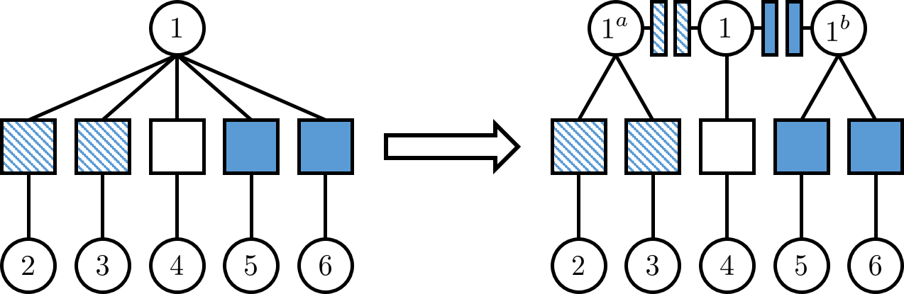
Figure 1: Renormalization process for mini-buckets $\mathcal{B}_{1}^{a}=\{\mathnormal{f}_{12},\mathnormal{f}_{13}\},\mathcal{B}_{1}^{b}=\{\mathnormal{f}_{15},\mathnormal{f}_{16}\}$ and $\mathcal{B}_{1}^{c}=\{\mathnormal{f}_{14}\}$.

3.1 Algorithm Description

For each variable $i$ in the elimination order $o$, MBR partitions a bucket $\mathcal{B}_{i}$ into $m_{i}$ distinct mini-buckets $\{\mathcal{B}_{i}^{\ell}\}_{\ell=1}^{m_{i}}$ with maximal size bounded by $ibound$. Then for $\ell=1,\cdots,m_{i}-1$, mini-bucket $\mathcal{B}_{i}^{\ell}$ is “renormalized” through replacing vertex $i$ by its replicate $i^{\ell}$ and then introducing local factors $r_{i}^{\ell},r_{i^{\ell}}$ for error compensation, i.e.,

$$\widetilde{\mathcal{B}}_{i}^{\ell}\leftarrow\{\mathnormal{f}_{\alpha\setminus\{i\}\cup\{i^{\ell}\}}|\mathnormal{f}_{\alpha}\in\mathcal{B}_{i}^{\ell}\}\cup\{r_{i}^{\ell},r_{i^{\ell}}\}.$$

Here, $r_{i}^{\ell},r_{i^{\ell}}$ are local “compensating/renormalizing factors”, chosen to approximate the factor $\mathnormal{f}_{\mathcal{B}_{i}^{\ell}}=\prod_{\mathnormal{f}_{\alpha}\in\mathcal{B}_{i}^{\ell}}\mathnormal{f}_{\alpha}$ well, where MBE approximates it using (2) and (3). See Figure 1 for illustration of the renormalization process. Specifically, the local compensating/renormalizing factors are chosen by solving the following optimization:

$$\operatornamewithlimits{\mbox{min}}_{r_{i}^{\ell},r_{i^{\ell}}}\qquad\sum_{\mathbf{x}_{\mathcal{B}^{\ell}_{i}}}\left(\mathnormal{f}_{\mathcal{B}_{i}^{\ell}}(\mathbf{x}_{\mathcal{B}_{i}^{\ell}})-\widetilde{\mathnormal{f}}_{\mathcal{B}_{i}^{\ell}}(\mathbf{x}_{\mathcal{B}_{i}^{\ell}})\right)^{2},$$ (4)

where $\widetilde{\mathnormal{f}}_{\mathcal{B}_{i}^{\ell}}$ is the factor induced on $\mathbf{x}_{\mathcal{B}_{i}^{\ell}}$ from the renormalized mini-bucket $\widetilde{\mathcal{B}}_{i}^{\ell}$:

$$\widetilde{\mathnormal{f}}_{\mathcal{B}_{i}^{\ell}}(\mathbf{x}_{\mathcal{B}_{i}^{\ell}}) =\sum_{x_{i}^{\ell}}\prod_{\mathnormal{f}_{\alpha}\in\widetilde{\mathcal{B}}_{i}^{\ell}}\mathnormal{f}_{\alpha}(\mathbf{x}_{\alpha})$$

$$=r_{i}^{\ell}(x_{i})\sum_{x_{i^{\ell}}}r_{i^{\ell}}(x_{i^{\ell}})\prod_{\mathnormal{f}_{\alpha}\in\mathcal{B}_{i}^{\ell}}\mathnormal{f}_{\alpha}(x_{i^{\ell}},\mathbf{x}_{\alpha\setminus\{i\}\cup\{i^{\ell}\}}).$$

We show that (4) can be solved efficiently in Section 3.2. After all mini-buckets are processed, factors can be summed over the variables $x_{i^{1}},\cdots,x_{i^{m_{i}-1}}$ and $x_{i}$ separately, i.e., introduce new factors as follows:

$$\mathnormal{f}_{\mathcal{B}_{i}^{\ell}\setminus\{i\}}(\mathbf{x}_{\mathcal{B}_{i}^{\ell}\setminus\{i\}}) =\sum_{x_{i^{\ell}}}\prod_{\mathnormal{f}_{\alpha}\in\widetilde{\mathcal{B}}_{i}^{\ell}\setminus\{r_{i}^{\ell}\}}\mathnormal{f}_{\alpha}(\mathbf{x}_{\alpha}),$$ (5)

$$=\sum_{x_{i^{\ell}}}r^{\ell}_{i}(x_{i^{\ell}})\prod_{\mathnormal{f}_{\alpha}\in\mathcal{B}_{i}^{\ell}}\mathnormal{f}_{\alpha}(x_{i^{\ell}},\mathbf{x}_{\alpha\setminus\{i\}\cup\{i^{\ell}\}}),$$

for $\ell=1,\cdots,m_{i}-1$ and

$$\mathnormal{f}_{\mathcal{B}_{i}^{m_{i}}\setminus\{i\}}(\mathbf{x}_{\mathcal{B}_{i}^{m_{i}}\setminus\{i\}})=\sum_{x_{i}}\prod_{\ell=1}^{m_{i}-1}r^{\ell}_{i}(x_{i^{\ell}})\prod_{\mathnormal{f}_{\alpha}\in\mathcal{B}_{i}^{m_{i}}}\mathnormal{f}_{\alpha}(\mathbf{x}_{\alpha}).$$ (6)

Resulting factors are then added to its corresponding mini-bucket and repeat until all buckets are processed, like BE and MBE. Here, one can check that

$$\prod_{\ell=1}^{m_{i}}\mathnormal{f}_{\mathcal{B}_{i}^{\ell}\setminus\{i\}}(\mathbf{x}_{\mathcal{B}_{i}^{\ell}\setminus\{i\}}) =\sum_{x_{i}}\mathnormal{f}_{\mathcal{B}_{i}^{m_{i}}}(\mathbf{x}_{\mathcal{B}_{i}^{m_{i}}})\prod_{\ell=1}^{m_{i}-1}\widetilde{\mathnormal{f}}_{\mathcal{B}_{i}^{\ell}}(\mathbf{x}_{\mathcal{B}_{i}^{\ell}}),$$

$$\approx\sum_{x_{i}}\prod_{\ell=1}^{m_{i}}\mathnormal{f}_{\mathcal{B}_{i}^{\ell}}(\mathbf{x}_{\mathcal{B}_{i}^{\ell}}),$$

from (4) and MBR indeed approximates BE. The formal description of MBR is given in Algorithm 2.

Algorithm 2 Mini-bucket renormalization (MBR)

1:  Input: GM $\mathcal{M}^{\dagger}=(\mathcal{G}^{\dagger},\mathcal{F}^{\dagger})$, elimination order $o$ and induced width bound $ibound$.  

2:  $\mathcal{F}\leftarrow\mathcal{F}^{\dagger}$

3:  for $i$ in $o$ do

4:     $\mathcal{B}_{i}\leftarrow\{\mathnormal{f}_{\alpha}|\mathnormal{f}_{\alpha}\in\mathcal{F},i\in\alpha\}$

5:     Divide $\mathcal{B}_{i}$ into $m_{i}$ subgroups $\{\mathcal{B}_{i}^{\ell}\}_{\ell=1}^{m_{i}}$ such that $|\mathcal{V}(\mathcal{B}_{i}^{\ell})|\leq ibound+1$ for $\ell=1,\cdots,m_{i}$.

6:     for $\ell=1,\cdots,m_{i}-1$ do

7:        Generate compensating factors $r_{i}^{\ell},r_{i^{\ell}}$ by (4).

8:        Generate new factor $\mathnormal{f}_{\mathcal{B}_{i}^{\ell}\setminus\{i\}}$ by (5).

9:     end for

10:     Generate new factor $\mathnormal{f}_{\mathcal{B}_{i}^{m_{i}}\setminus\{i\}}$ by (6).

11:     for $\ell=1,\cdots,m_{i}$ do

12:        $\mathcal{F}\leftarrow\mathcal{F}\cup\{\mathnormal{f}_{\mathcal{B}_{i}^{\ell}\setminus\{i\}}\}\setminus\mathcal{B}_{i}^{\ell}$

13:     end for

14:  end for  

15:  Output: $Z=\prod_{\mathnormal{f}_{\alpha}\in\mathcal{F}}\mathnormal{f}_{\alpha}$

3.2 Complexity

The optimization (4) is related to the rank-$1$ approximation on $\mathnormal{f}_{\mathcal{B}_{i}^{\ell}}$, which can be solved efficiently via (truncated) singular value decomposition (SVD). Specifically, let $\mathbf{M}$ be a $d\times d^{|\mathcal{V}(\mathcal{B}_{i}^{\ell})|-1}$ matrix representing $\mathnormal{f}_{\mathcal{B}_{i}^{\ell}}$ as follows:

$$\mathbf{M}\left(x_{i},\sum_{j\in\mathcal{V}(\mathcal{B}_{i}^{\ell}),j\neq i}x_{j}\prod_{k\in\mathcal{V}(\mathcal{B}_{i}^{\ell}),k>j}d\right)=\mathnormal{f}_{\mathcal{B}_{i}^{\ell}}(\mathbf{x}_{\mathcal{B}_{i}^{\ell}}).$$ (7)

Then rank-1 truncated SVD for $\mathbf{M}$ solves the following optimization:

$$\min_{\mathbf{r}_{1},\mathbf{r}_{2}}\lVert\mathbf{M}-\mathbf{r}_{1}\mathbf{r}_{2}^{\top}\mathbf{M}\rVert_{F},$$

where optimization is over $d$-dimensional vectors $\mathbf{r}_{1},\mathbf{r}_{2}$ and $\lVert\cdot\rVert_{F}$ denotes the Frobenious norm. Namely, the solution $\mathbf{r}_{1}=\mathbf{r}_{2}$ becomes the most significant (left) singular vector of $\mathbf{M}$, associated with the largest singular value. Especially, since $\mathbf{M}$ is a non-negative matrix, its most significant singular vector is always non-negative due to the Perron-Frobenius theorem (Perron, 1907). By letting $r_{i^{\ell}}(x)=\mathbf{r}_{1}(x)$ and $r_{i}^{\ell}(x)=\mathbf{r}_{2}(x)$, one can check that this optimization is equivalent to (4), where in fact, $r_{i^{\ell}}(x)=r_{i}^{\ell}(x)$, i.e., they share the same values. Due to the above observations, the complexity of (4) is $N_{\text{SVD}}(\mathbf{M})$ that denotes the complexity of SVD for matrix $\mathbf{M}$. Therefore, the overall complexity becomes

$$O\left(N_{SVD}(\mathbf{M})\cdot T\right)=O\left(N_{\text{SVD}}(\mathbf{M})\cdot|\mathcal{E}|\cdot\max_{\alpha\in\mathcal{E}}|\alpha|\right),$$

where $N_{\text{SVD}}(\mathbf{M})=O(d^{ibound+2})$ in general, but typically much faster in the existing SVD solver.

4 Global-Bucket Renormalization

In the previous section, MBR only considers the local neighborhood for renormalizing mini-buckets to approximate a single marginalization process of BE. Here we extend the approach and propose global-bucket renormalization (GBR), which incorporates a global perspective. The new scheme re-updates the choice of compensating local factors obtained in MBR by considering factors that were ignored during the original process. In particular, GBR directly minimizes the error in the partition function from each renormalization, aiming for improved accuracy compared to MBR.

4.1 Intuition and Key-Optimization

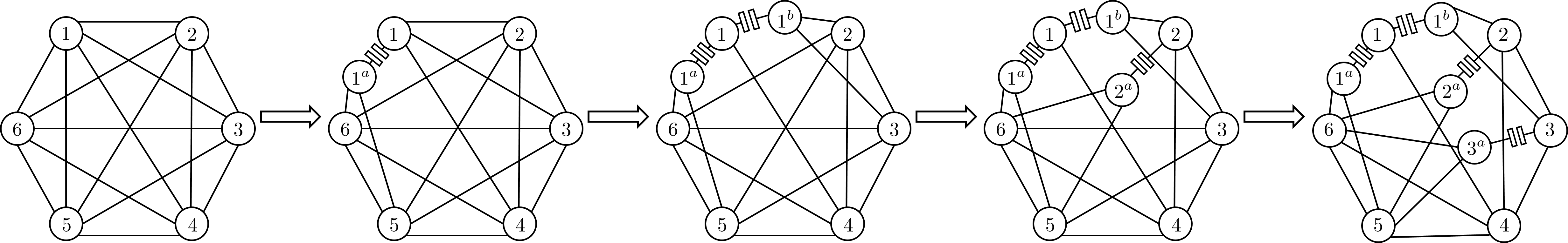
Figure 2: Example of GM renormalization on complete graph with size $|\mathcal{V}|=6$ corresponding to execution of MBR with elimination order $o=1,\cdots,6$ and $ibound=2$. Here, pairwise factors between variables are assumed to exist inside edges. Partition function of final GM is able to be computed from BE with induced width $2$ and elimination order $\widetilde{o}=[1^{a},1^{b},1,2^{a},2,3^{a},3,4,5,6]$.

Renormalized GMs in MBR. For providing the underlying design principles of GBR, we first track an intermediate estimation of the partition function made during MBR by characterizing the corresponding sequence of renormalized GMs. Specifically, we aim for constructing a sequence of $T+1$ GMs $\mathcal{M}^{(1)},\cdots,\mathcal{M}^{(T+1)}$ with $T=\sum_{i=1}^{n}(m_{i}-1)$ by breaking each $i$-th iteration of MBR into $m_{i}-1$ steps of GM renormalizations, $\mathcal{M}^{(1)}$ is the original GM, and each transition from $\mathcal{M}^{(t)}$ to $\mathcal{M}^{(t+1)}$ corresponds to renormalization of some mini-bucket $\mathcal{B}_{i}^{\ell}$ to $\widetilde{\mathcal{B}}_{i}^{\ell}$. Then, the intermediate estimation for the original partition function $Z$ at the $t$-th step is partition function $Z^{(t)}$ of $\mathcal{M}^{(t)}$ where the last one $Z^{(T+1)}$ is the output of MBR.

To this end, we introduce “scope” for each factor $\mathnormal{f}_{\alpha}$ appearing in MBR to indicate which parts of GM are renormalized at each step. In particular, the scope $\mathcal{S}_{\mathnormal{f}_{\alpha}}=(\mathcal{G}_{\mathnormal{f}_{\alpha}},\mathcal{F}_{\mathnormal{f}_{\alpha}})$ consists of a graph $\mathcal{G}_{\mathnormal{f}_{\alpha}}=(\mathcal{V}_{\mathnormal{f}_{\alpha}},\mathcal{E}_{\mathnormal{f}_{\alpha}})$ and set of factors $\mathcal{F}_{\mathnormal{f}_{\alpha}}$ that are associated to $\mathnormal{f}_{\alpha}$ as follows:

$$\mathnormal{f}_{\alpha}(\mathbf{x}_{\alpha})=\sum_{\mathbf{x}_{\mathcal{V}_{\mathnormal{f}_{\alpha}}\setminus\alpha}}\prod_{\mathnormal{f}_{\beta}\in\mathcal{F}_{\mathnormal{f}_{\alpha}}}\mathnormal{f}_{\beta}(\mathbf{x}_{\beta}).$$

Initially, scopes associated with initial factors are defined by themselves, i.e.,

$$\mathcal{S}_{\mathnormal{f}_{\alpha}}\leftarrow((\alpha,\{\alpha\}),\{\mathnormal{f}_{\alpha}\}),$$ (8)

for each factor $\mathnormal{f}_{\alpha}$ of $\mathcal{M}^{(1)}$, and others of $\mathcal{M}^{(t)}=((\mathcal{V}^{(t)},\mathcal{E}^{(t)}),\mathcal{F}^{(t)})$ with $t\geq 2$ are to be defined iteratively under the MBR process, as we describe in what follows.

Consider the $t$-th iteration of MBR, where mini-bucket $\mathcal{B}_{i}^{\ell}$ is being renormalized into $\widetilde{\mathcal{B}}_{i}^{\ell}$. Then scope $\mathcal{S}_{\mathnormal{f}}$ for all $\mathnormal{f}\in\mathcal{B}_{i}^{\ell}$ goes through renormalization by replacing every $i$ in the scope by $i^{\ell}$ as follows:

$$\widetilde{S}_{\mathnormal{f}}\leftarrow(\mathcal{V}_{\mathnormal{f}}\setminus\{i\}\cup\{i^{\ell}\},\{\bar{\alpha}|\alpha\in\mathcal{E}_{\mathnormal{f}}\},\{\mathnormal{f}_{\bar{\alpha}}|\mathnormal{f}_{\alpha}\in\mathcal{F}_{\mathnormal{f}}\}),$$ (9)

where $\bar{\alpha}=\begin{cases}\alpha\setminus\{i\}\cup\{i^{\ell}\}&\mbox{ if}~{}i\in\alpha\\ \qquad\alpha&\mbox{otherwise}\end{cases}$. Then, the respective GM is renormalized accordingly for the change of scopes, in addition to compensating factors $r_{i}^{\ell},r_{i^{\ell}}$:

$$\mathcal{V}^{(t+1)} \leftarrow\mathcal{V}^{(t)}\cup\{i^{\ell}\},$$

$$\mathcal{E}^{(t+1)} \leftarrow\mathcal{E}^{(t)}\setminus\mathcal{E}_{\mathcal{B}_{i}^{\ell}}\cup\widetilde{\mathcal{E}}_{\mathcal{B}_{i}^{\ell}}\cup\{\{i\},\{i^{\ell}\}\},$$ (10)

$$\mathcal{F}^{(t+1)} \leftarrow\mathcal{F}^{(t)}\setminus\mathcal{F}_{\mathcal{B}_{i}^{\ell}}\cup\widetilde{\mathcal{F}}_{\mathcal{B}_{i}^{\ell}}\cup\{r_{i}^{\ell},r_{i^{\ell}}\},$$

where $\mathcal{E}_{\mathcal{B}_{i}^{\ell}}=\cup_{\mathnormal{f}\in\mathcal{B}_{i}^{\ell}}\mathcal{E}_{\mathnormal{f}},$ and other union of scope components $\widetilde{\mathcal{E}}_{\mathcal{B}_{i}^{\ell}},\mathcal{V}_{\mathcal{B}_{i}^{\ell}},\widetilde{\mathcal{V}}_{\mathcal{B}_{i}^{\ell}},\mathcal{F}_{\mathcal{B}_{i}^{\ell}},\widetilde{\mathcal{F}}_{\mathcal{B}_{i}^{\ell}}$ are defined similarly. Finally, scope $\mathcal{S}_{\mathnormal{f}_{\mathcal{B}_{i}^{\ell}\setminus\{i\}}}$ for newly generated factors $\mathnormal{f}_{\mathcal{B}_{i}^{\ell}\setminus\{i\}}$ is

$$\mathcal{S}_{\mathnormal{f}_{\mathcal{B}_{i}^{\ell}\setminus\{i\}}}\leftarrow((\widetilde{\mathcal{V}}_{\mathcal{B}_{i}^{\ell}},\widetilde{\mathcal{E}}_{\mathcal{B}_{i}^{\ell}}\cup\{\{i^{\ell}\}\}),\widetilde{\mathcal{F}}_{\mathcal{B}_{i}^{\ell}}\cup\{r_{i^{\ell}}\}).$$ (11)

Furthermore, if $\ell=m_{i}-1$, we have

$$\mathcal{S}_{\mathnormal{f}_{\mathcal{B}_{i}^{m_{i}}\setminus\{i\}}}\leftarrow((\mathcal{V}_{\mathcal{B}_{i}^{m_{i}}},\mathcal{E}_{\mathcal{B}_{i}^{m_{i}}}\cup\{\{i\}\}),\mathcal{F}_{\mathcal{B}_{i}^{m_{i}}}\cup\{r_{i}^{\ell}\}_{\ell=1}^{m_{i}-1}).$$ (12)

This is repeated until the MBR process terminates, as formally described in Algorithm 3. By construction, the output of MBR is equal to the partition function of the last GM $\mathcal{M}^{(T+1)}$, which is computable via BE with induced width smaller than $ibound+1$ given elimination order

$$\widetilde{o}=[1^{1},\cdots,1^{m_{1}-1},1,\cdots,n^{1},\cdots,n^{m_{n}-1},n].$$ (13)

See Algorithm 3 for the formal description of this process, and Figure 2 for an example.

Optimizing intermediate approximations. Finally, we provide an explicit optimization formulation for minimizing the change of intermediate partition functions in terms of induced factors. Specifically, for each $t$-th renormalization, i.e., from $\mathcal{M}^{(t)}$ to $\mathcal{M}^{(t+1)}$, we consider change of the following factor $\mathnormal{f}_{i}$ induced from global-bucket $\mathcal{F}^{(t)}$ to variable $x_{i}$ in a “skewed” manner as follows:

$$\mathnormal{f}_{i}(x_{i}^{(1)},x_{i}^{(2)}):= \sum_{\mathbf{x}_{\mathcal{V}^{(t)}\setminus\{i\}}}\prod_{\mathnormal{f}_{\alpha}\in\mathcal{F}_{\mathcal{B}_{i}^{\ell}}}\mathnormal{f}_{\alpha}(x_{i}^{(1)},\mathbf{x}_{\alpha\setminus\{i\}})$$

$$\cdot\prod_{\mathnormal{f}_{\alpha}\in\mathcal{F}^{(t)}\setminus\mathcal{F}_{\mathcal{B}_{i}^{\ell}}}\mathnormal{f}_{\alpha}(x_{i}^{(2)},\mathbf{x}_{\alpha\setminus\{i\}}),$$

where $x_{i}^{(1)},x_{i}^{(2)}$ are the newly introduced “split variables” that are associated with the same vertex $i$, but allowed to have different values for our purpose. Next, the bucket $\mathcal{F}^{(t)}$ is renormalized into $\mathcal{F}^{(t+1)}$, leading to the induced factor of $\widetilde{\mathnormal{f}}_{i}$ defined as follows:

$$\widetilde{\mathnormal{f}}_{i}(x_{i}^{(1)},x_{i}^{(2)}):= \sum_{\mathbf{x}_{\mathcal{V}^{(t+1)}\setminus\{i\}}}\prod_{\mathnormal{f}_{\alpha}\in\widetilde{\mathcal{F}}_{\mathcal{B}_{i}^{\ell}}\cup\{r_{i}^{\ell},r_{i^{\ell}}\}}\mathnormal{f}_{\alpha}(x_{i}^{(1)},\mathbf{x}_{\alpha\setminus\{i\}})$$

$$\cdot\prod_{\mathnormal{f}_{\alpha}\in\mathcal{F}^{(t+1)}\setminus\widetilde{\mathcal{F}}_{\mathcal{B}_{i}^{\ell}}\setminus\{r_{i}^{\ell},r_{i^{\ell}}\}}\mathnormal{f}_{\alpha}(x_{i}^{(2)},\mathbf{x}_{\alpha\backslash\{i\}})$$

$$= r_{i}^{\ell}(x_{i}^{(1)})\sum_{x_{i^{\ell}}}r_{i^{\ell}}(x_{i^{\ell}})\mathnormal{f}_{i}(x_{i^{\ell}},x_{i}^{(2)}).$$

Then change in $\mathnormal{f}_{i}$ is directly related with change in partition function since $Z^{(t-1)}$ and $Z^{(t)}$ can be described as follows:

$$Z^{(t-1)}=\sum_{x_{i}}\mathnormal{f}_{i}(x_{i},x_{i}),\quad Z^{(t)}=\sum_{x_{i}}\widetilde{\mathnormal{f}}_{i}(x_{i},x_{i}).$$

Consequently, GBR chooses to minimize the change in $\mathnormal{f}_{i}$ by re-updating $r_{i}^{\ell},r_{i^{\ell}}$, i.e., it solves

$$\min_{r_{i}^{\ell},r_{i^{\ell}}}\sum_{x_{i}^{(1)},x_{i}^{(2)}}\bigg{(}\mathnormal{f}_{i}(x_{i}^{(1)},x_{i}^{(2)})-\widetilde{\mathnormal{f}}_{i}(x_{i}^{(1)},x_{i}^{(2)})\bigg{)}^{2}.$$ (14)

However, we remark that (14) is intractable since its objective is “global”, and requires summation over all variables except one, i.e., $\mathbf{x}_{\mathcal{V}^{(t)}\setminus\{i\}}$, and this is the key difference from (4) which seeks to minimize the error described by the local mini-bucket. GBR avoids this issue by substituting $\mathnormal{f}_{i}$ by its tractable approximation $\mathnormal{g}_{i}$, which is to be described in the following section.

Algorithm 3 GM renormalization

1:  Input: GM $\mathcal{M}^{\dagger}=(\mathcal{G}^{\dagger},\mathcal{F}^{\dagger})$, elimination order $o$ and induced width bound $ibound$.  

2:  $\mathcal{M}^{(1)}\leftarrow\mathcal{M}^{\dagger}$

3:  Run Algorithm 2 with input $\mathcal{M}^{(1)},o,ibound$ to obtain mini-buckets $\mathcal{B}_{i}^{\ell}$ and compensating factors $r_{i}^{\ell},r_{i^{\ell}}$ for $i=1,\cdots,n$ and $\ell=1,\cdots,m_{i}$.

4:  for $\mathnormal{f}\in\mathcal{F}^{(1)}$ do

5:     Assign scope $\mathcal{S}_{\mathnormal{f}}$ for $\mathnormal{f}$ by (8).

6:  end for

7:  for $i$ in $o$ do

8:     for $\ell=1,\cdots,m_{i}-1$ do

9:        for $\mathnormal{f}\in\mathcal{B}_{i}^{\ell}$ do

10:           Renormalize scope $\mathcal{S}_{\mathnormal{f}}$ for $\mathnormal{f}$ into $\widetilde{\mathcal{S}}_{\mathnormal{f}}$ by (9).

11:        end for

12:        Set $t=\sum_{j=1}^{i-1}(m_{i}-1)+\ell$.

13:        Renormalize GM $\mathcal{M}^{(t)}$ into $\mathcal{M}^{(t+1)}$ by (10).

14:        Assign scope $\mathcal{S}_{\mathnormal{f}_{\mathcal{B}_{i}^{\ell}\setminus\{i\}}}$ for factor $\mathnormal{f}_{\mathcal{B}_{i}^{\ell}\setminus\{i\}}$ by (11).

15:     end for

16:     Assign scope $\mathcal{S}_{\mathnormal{f}_{\mathcal{B}_{i}^{m_{i}}\setminus\{i\}}}$ for factor $\mathnormal{f}_{\mathcal{B}_{i}^{m_{i}}\setminus\{i\}}$ by (12).

17:  end for  

18:  Output: Final GM $\mathcal{M}^{(T+1)}$ with $T=\sum_{i=1}^{n}(m_{i}-1)$.

4.2 Algorithm Description

In this section, we provide a formal description of GBR. First, consider the sequence of GMs $\mathcal{M}^{(1)},\cdots,\mathcal{M}^{(T+1)}$ from interpreting MBR as GM renormalizations. One can observe that this corresponds to $T$ choices of compensating factors made at each renormalization, i.e., $r^{(1)},\cdots,r^{(T)}$ where $r^{(t)}(x)=r_{i}^{\ell}(x)=r_{i^{\ell}}(x)$ for the associated replicate vertex $i^{\ell}$. GBR modifies this sequence iteratively by replacing intermediate choice of compensation $r^{(t)}$ by another choice $s^{(t)}(x)=s_{i}^{\ell}(x)=s_{i^{\ell}}(x)$ in reversed order, approximately solving (14) until all compensating factors are updated. Then, GBR outputs partition function $Z^{(T+1)}$ for $\mathcal{M}^{(T+1)}$ as an approximation of the original partition function $Z$.

Now we describe the process of choosing new compensating factors $s_{i}^{\ell},s_{i^{\ell}}$ at $t^{\prime}$-th iteration of GBR by approximately solving (14). To this end, the $t^{\prime}$-th choice of compensating factors are expressed as follows:

$$r^{(1)},\cdots,r^{(t)},s^{(t+1)},\cdots,s^{(T)},$$ (15)

with $t=T-t^{\prime}+1$ and $s^{(t+1)},\cdots,s^{(T)}$ already chosen in the previous iteration of GBR. Next, consider sequence of GMs $\widehat{\mathcal{M}}^{(1)},\cdots,\widehat{\mathcal{M}}^{(T+1)}$ that were generated similarly with GM renormalization corresponding to MBR, but with compensating factors chosen by (15). Observe that the first $t$ renormalizations of GM correspond to those of MBR since the updates are done in reverse order, i.e., $\widehat{\mathcal{M}}^{(t^{\prime})}=\mathcal{M}^{(t^{\prime})}$ for $t^{\prime}<t+1$. Next, $\mathnormal{f}_{i}$ in (4) is expressed as summation over $\mathbf{x}_{\widehat{\mathcal{V}}^{(t+1)}\setminus\{i,i^{\ell}\}}^{\ell}$ in $\widehat{\mathcal{M}}^{(t+1)}$, defined as follows:

$$\mathnormal{f}_{i}(x_{i^{\ell}},x_{i})=\sum_{\mathbf{x}_{\widehat{\mathcal{V}}^{(t+1)}\setminus\{i,i^{\ell}\}}}\prod_{\mathnormal{f}_{\alpha}\in\widehat{\mathcal{F}}^{(t+1)}\setminus\{r_{i}^{\ell},r_{i^{\ell}}\}}\mathnormal{f}_{\alpha}(\mathbf{x}_{\alpha}).$$

Since $\mathnormal{f}_{i}$ resembles the partition function in a way that it is also a summation over GM with small change in a set of factors, i.e., excluding local factors $r_{i}^{\ell},r_{i^{\ell}}$, we expect $\mathnormal{f}_{i}$ to be approximated well by a summation $g_{i}$ over $\mathbf{x}_{\widehat{\mathcal{V}}^{(T+1)}\setminus\{i,i^{\ell}\}}$ in $\widehat{\mathcal{M}}^{(T+1)}$:

$$g_{i}(x_{i^{\ell}},x_{i}):=\sum_{\mathbf{x}_{\widehat{\mathcal{V}}^{(T+1)}\setminus\{i,i^{\ell}\}}}\prod_{\mathnormal{f}_{\alpha}\in\widehat{\mathcal{F}}^{(T+1)}\setminus\{r_{i}^{\ell},r_{i^{\ell}}\}}\mathnormal{f}_{\alpha}(\mathbf{x}_{\alpha}),$$

which can be computed in $O(|\mathcal{E}|d^{ibound+2})$ complexity via appying BE in $\widehat{\mathcal{M}}^{(T+1)}$ with elimination order $\widetilde{o}\setminus\{i,i^{\ell}\}$ as in (13). Then the following optimization is obtained as an approximation of (14):

$$\min_{s_{i}^{\ell},s_{i^{\ell}}}\sum_{x_{i}^{(1)},x_{i}^{(2)}}\bigg{(}g_{i}(x_{i}^{(1)},x_{i}^{(2)})-\widetilde{g}_{i}(x_{i}^{(1)},x_{i}^{(2)})\bigg{)}^{2},$$ (16)

where $\widetilde{g}_{i}$ corresponds to renormalized factor $\widetilde{\mathnormal{f}}_{i}$:

$$\widetilde{g}_{i}(x_{i^{\ell}},x_{i}):=s_{i}^{\ell}(x_{i^{\ell}})\sum_{x_{i^{\ell}}}s_{i^{\ell}}(x_{i^{\ell}})g_{i}(x_{i^{\ell}},x_{i}).$$

As a result, one can expect choosing compensating factors from (16) to improve over that of (4) as long as MBR provides reasonable approximation for $\mathnormal{f}_{i}$. The optimization is again solvable via rank-$1$ truncated SVD and the overall complexity of GBR is

$$O\left(d^{ibound+2}N_{\text{SVD}}(\mathbf{M}^{\text{global}})\cdot|\mathcal{E}|^{2}\cdot\max_{\alpha\in\mathcal{E}}|\alpha|^{2}\right),$$

where $N_{\text{SVD}}(\mathbf{M}^{\text{global}})=O(d^{3})$ is the complexity for performing SVD on $d\times d$ matrix $\mathbf{M}^{\text{global}}$ representing function $g$ as in (7). While the formal description of GBR is conceptually a bit complicated, one can implement it efficiently. Specifically, during the GBR process, it suffices to keep only the description of renormalized GM $\mathcal{M}^{(T+1)}$ with an ongoing set of compensating factors, e.g., (15), in order to update compensating factors iteratively by (16). The formal description of the GBR scheme is provided in Algorithm 4.

Algorithm 4 Global-Bucket Renormalization (GBR)

1:  Input: GM $\mathcal{M}^{\dagger}=(G^{\dagger},\mathcal{F}^{\dagger})$, elimination order $o$ and induced width bound $ibound$.  

2:  Run Algorithm 3 with input $\mathcal{M}^{\dagger},o,ibound$ to obtain renormalized GM $\mathcal{M}$ and compensating factors $r_{i}^{\ell}$ for $i=1,\cdots,n$ and $\ell=1,\cdots,m_{i}$.

3:  Set the renormalized elimination order as follows:

$$\widetilde{o}=[1^{1},\cdots,1^{m_{1}-1},1,\cdots,n^{1},\cdots,n^{m_{n}-1},n].$$

4:  for $i^{\ell}=n^{m_{n}-1},\cdots,n^{1},\cdots,1^{m_{1}-1},\cdots,1^{1}$ do

5:     Generate $s_{i}^{\ell},s_{i}^{\ell}$ by solving

$$\min_{s_{i}^{\ell},s_{i^{\ell}}} \sum_{x_{i}^{(1)},x_{i}^{(2)}}\bigg{(}g_{i}(x_{i}^{(1)},x_{i}^{(2)})-\widetilde{g}_{i}(x_{i}^{(1)},x_{i}^{(2)})\bigg{)}^{2},$$

6:     where $g_{i},\widetilde{g}_{i}$ is defined as follows:

$$g_{i}(x_{i^{\ell}},x_{i}) =\sum_{\mathbf{x}_{\mathcal{V}\setminus\{i,i^{\ell}\}}}\prod_{\mathnormal{f}_{\alpha}\in\mathcal{F}\setminus\{r_{i}^{\ell},r_{i^{\ell}}\}}\mathnormal{f}_{\alpha}(\mathbf{x}_{\alpha}),$$

$$\widetilde{g}_{i}(x_{i^{\ell}},x_{i}) =s_{i}^{\ell}(x_{i^{\ell}})\sum_{x_{i}^{\ell}}s_{i^{\ell}}(x_{i}^{\ell})g_{i}(x_{i}^{\ell},x_{i}),$$

with its computation done by BE with elimination order of $\widetilde{o}\setminus\{i,i^{\ell}\}$.

7:     Update GM $\mathcal{M}$ by $\mathcal{F}\leftarrow\mathcal{F}\setminus\{r_{i}^{\ell},r_{i^{\ell}}\}\cup\{s_{i}^{\ell},s_{i^{\ell}}\}$.

8:  end for

9:  Get $Z=\sum_{\mathbf{x}}\prod_{\mathnormal{f}_{\alpha}\in\mathcal{F}}\mathnormal{f}_{\alpha}(\mathbf{x}_{\alpha})$ via BE with elimination order $\widetilde{o}$.  

10:  Output: $Z$

5 Experimental Results

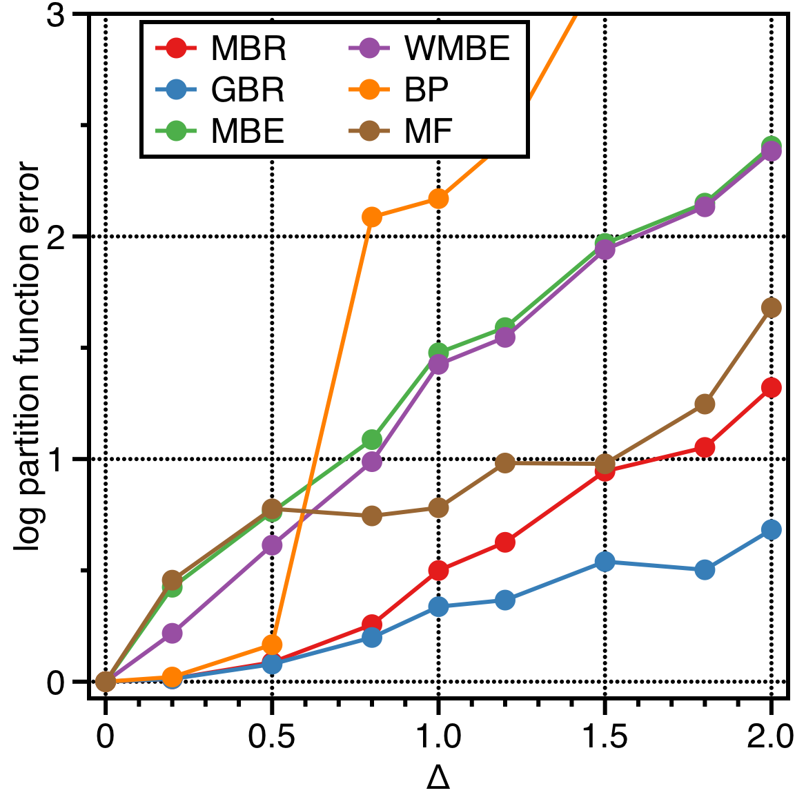
(a) Complete graph, $|\mathcal{V}|=15$

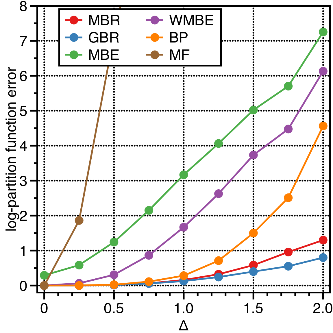
(b) Grid graph $15\times 15$

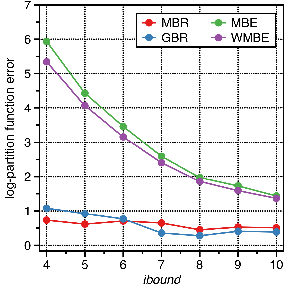
(c) Complete graph, $|\mathcal{V}|=15$

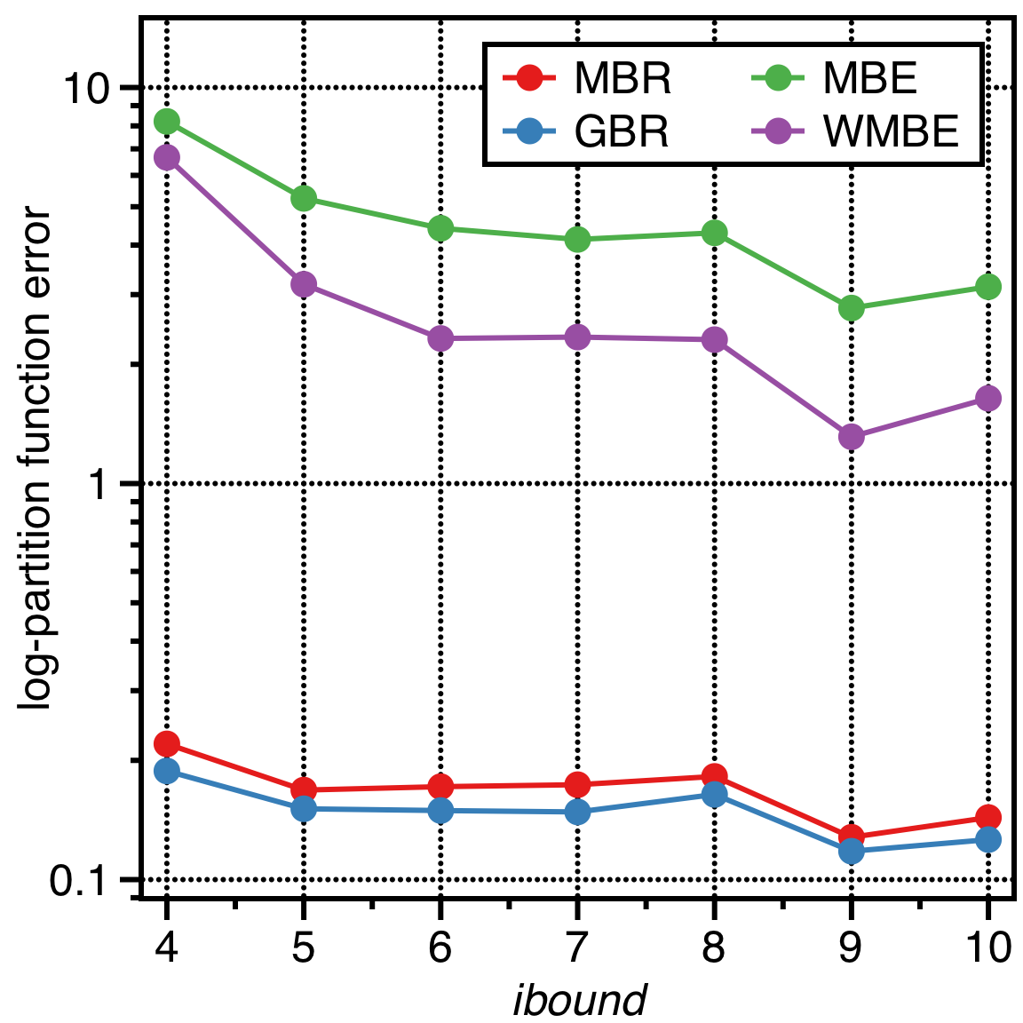
(d) Grid graph $15\times 15$

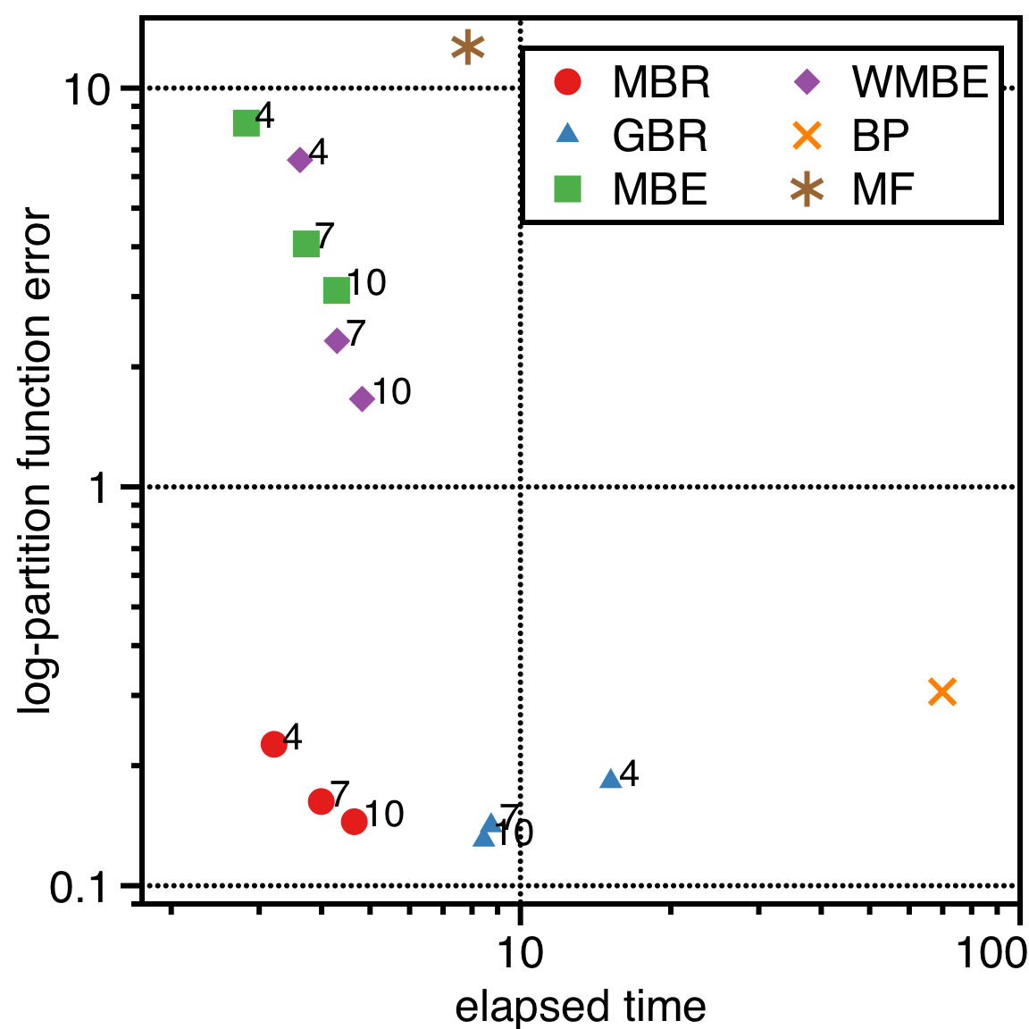
(e) Grid graph $15\times 15$

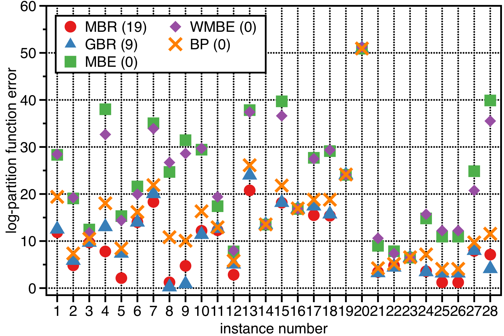
(f) Promedus dataset

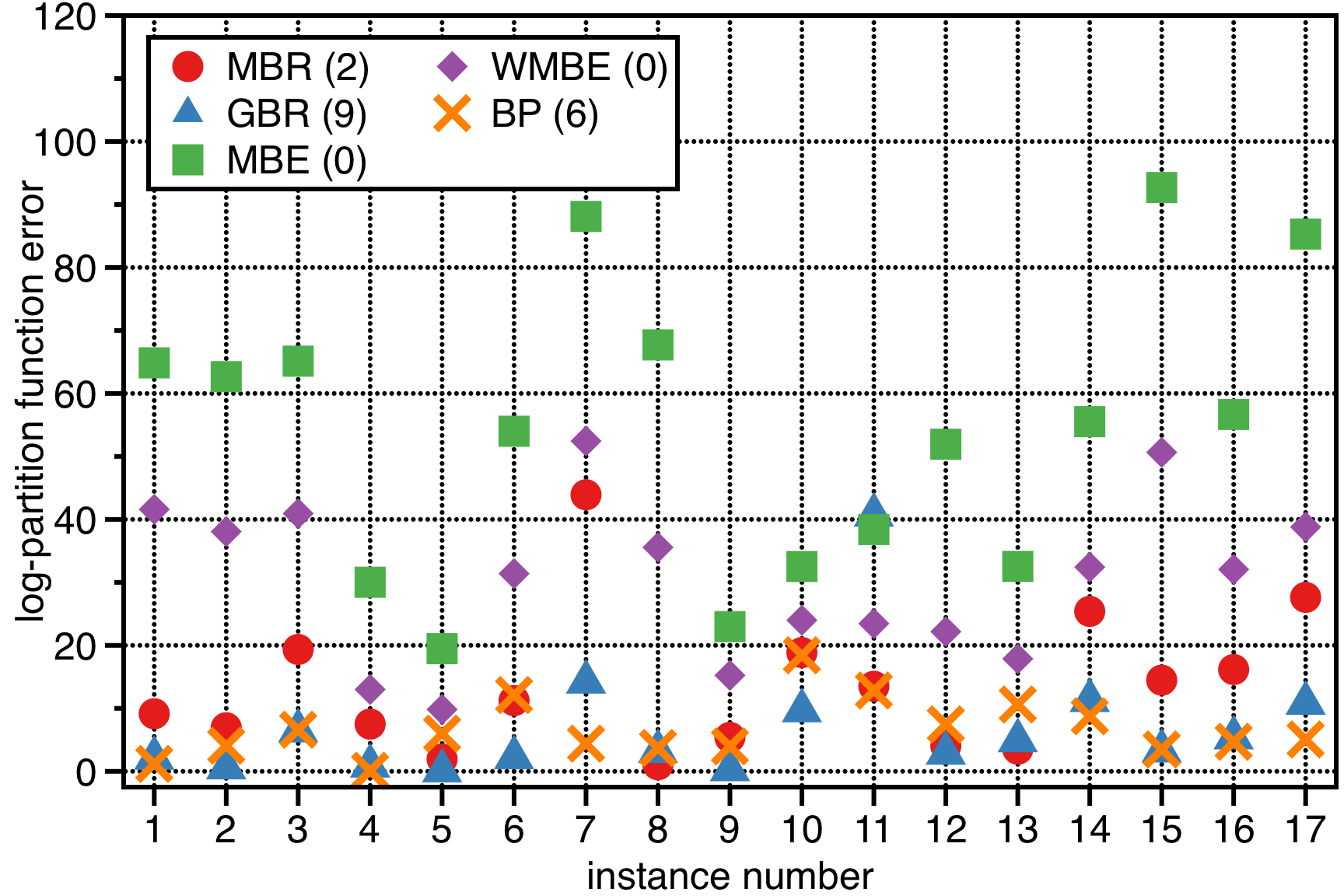
(g) Linkage dataset

Figure 3: Performance comparisons under (3(a), 3(b)) varying interaction strength parameter $\Delta$, and (3(c), 3(d)) induced width bound $ibound$. Ising models are either defined on (3(a), 3(c)) complete graphs with $|\mathcal{V}|=15$ or (3(b), 3(d)) grid graphs with $|\mathcal{V}|=225$. Each plot is averaged over $100$ models. (3(e)) reports the averaged error versus elapsed time while varying $ibound$ in the same setting as (3(d)), where number labels by points indicate the corresponding $ibound$ used. Numbers in brackets, e.g., MBR(19), count the instances of each algorithm to win in terms of approximation accuracy under (3(f)) Promedus and (3(g)) Linkage datasets.

In this section, we report experimental results on performance of our algorithms for approximating the partition function $Z$. Experiments were conducted for Ising models defined on grid-structured and complete graphs as well as two real-world datasets from the UAI 2014 Inference Competition (Gogate, 2014). We compare our mini-bucket renormalization (MBR) and global-bucket renormalization (GBR) scheme with other mini-bucket algorithms, i.e., mini-bucket elimination (MBE) by Dechter & Rish (2003) and weighted mini-bucket elimination (WMBE) by Liu & Ihler (2011). Here, WMBE used uniform Hölder weights, with additional fixed point reparameterization updates for improving its approximation, as proposed by Liu & Ihler, 2011. For all mini-bucket algorithms, we unified the choice of elimination order for each instance of GM by applying min-fill heuristics (Koller & Friedman, 2009). Further, we also run the popular variational inference algorithms: mean-field (MF) and loopy belief propagation (BP), For performance measure, we use the log-partition function error, i.e., $|\log_{10}Z-\log_{10}Z_{\text{approx}}|$ where $Z_{\text{approx}}$ is the approximated partition function from a respective algorithm.

Ising models. We first consider the most popular binary pairwise GMs, called Ising models (Onsager, 1944): $p(\mathbf{x})=\frac{1}{Z}\exp\left(\sum_{i\in\mathcal{V}}\phi_{i}x_{i}+\sum_{(i,j)\in\mathcal{E}}\phi_{ij}x_{i}x_{j}\right),$ where $x_{i}\in\{-1,1\}$. In our experiments, we draw $\phi_{ij}$ and $\phi_{i}$ uniformly from intervals of $[-\Delta,\Delta]$ and $[-0.1,0.1]$ respectively, where $\Delta$ is a parameter controlling the ‘interaction strength’ between variables. As $\Delta$ grows, the inference task is typically harder. Experiments were conducted in two settings: complete graphs with $15$ variables ($105$ pairwise factors), and $15\times 15$ non-toroidal grid graphs ($225$ variables, $420$ pairwise factors). Both settings have moderate tree-width, enabling exact computation of the partition function using BE with induced widths of 15 and 16, respectively. We vary the interaction strength $\Delta$ and the induced width bound $ibound$ (for mini-bucket algorithms), where $ibound=10$ and $\Delta=1.0$ are the default choices. For each choice of parameters, results are obtained by averaging over 100 random model instances.

As shown in Figure 3(a)-3(d), both MBR and GBR perform impressively compared to MF and BP. Notably, the relative outperformance of our methods compared to the earlier approaches increases with $\Delta$ (more difficult instances), and as the bound of induced width gets smaller. This suggests that our methods scale well with the size and difficulty of GM. In Figure 3(c), where $ibound$ is varied for complete graphs, we observe that GBR does not improve over MBR when $ibound$ is small, but does so after $ibound$ grows large. This is consistent with our expectation that in order for GBR to improve over MBR, the initial quality of MBR should be acceptable. Our experimental setup on Ising grid GMs with varying interaction strength is identical to that of Xue et al. (2016), where they approximate variable elimination in the Fourier domain. Comparing results, one can observe that our methods significantly outperform their prior algorithm.

Figure 3(e) reports the trade-off between accuracy and elapsed time with varying $ibound$. Here, we observe that MBR is much faster than MBE or WMBE to reach a desired accuracy, i.e., MBR with $ibound=4$ is faster and more accurate than MBE and WMBE with $ibound>4$. Further, we also note that increasing $ibound$ for GBR does not lead to slower running time, while the accuracy is improved. This is because smaller $ibound$ increases the numbers of mini-buckets and corresponding SVD calls.

UAI datasets. We further show results of real-world models from the UAI 2014 Inference Competition, namely the Promedus (medical diagnosis) and Linkage (genetic linkage) datasets. Specifically, there exist $35$ instances of Promedus GMs in with the average of $544.75$ binary variables and $305.85$ non-singleton hyper-edges with averaged maximum size $\max_{\alpha\in\mathcal{E}}|\alpha|=3$. In case of Linkage GMs, there exist $17$ instances with the average of $949.94$ variables with averaged maximum cardinality $\max_{i\in\mathcal{V}}|\mathcal{X}_{i}|=4.95$ and $727.35$ non-singleton hyper-edges with averaged maximum size $\max_{\alpha\in\mathcal{E}}|\alpha|=4.47$. Again, induced width bounds for mini-bucket algorithms are set to $ibound=10$.

The experimental results are summarized in Figure 3(f) and 3(g). Here, results for MF was omitted since it is not able to run on these instances by its construction. First, in Promedus dataset, i.e., Figure 3(f), MBR and GBR clearly dominates over all other algorithms. Even when GBR fails to improve MBR, it still outperforms other algorithms. Next, in Figure 3(g), one can observe that MBR and GBR outperform other algorithms in $11/17=64\%$ of the Linkage instances and are always as nearly good as the best, i.e., BP, in other instances. In particular, our algorithms outperform over all previous mini-bucket variants and expected to outperform BP more significantly by choosing a larger $ibound$.

Guide for implementation. Based on the experiments, we provide useful recommendations for application of MBR and GBR. First, we emphasize that choosing the right elimination order is important for performance. Especially, min-fill heuristic improved the performance of MBR and GBR significantly, as with other mini-bucket algorithms. Further, whenever memory is available, running MBR with increased $ibound$ typically leads to better trade-off between complexity and performance than running GBR. When memory is limited, GBR is recommended for improving the approximation quality while using the same-order of memory.

6 Conclusion and Future Work

We developed a new family of mini-bucket algorithms, MBR and GBR, inspired by the tensor network renormalization framework in statistical physics. The proposed schemes approximate the variable elimination process efficiently by repeating low-rank projections of mini-buckets. Extensions to higher-order low-rank projections (Xie et al., 2012; Evenbly, 2017) might improve performance. GBR calibrates MBR via minimization of renormalization error for the partition function explicitly. A similar optimization was considered in the so-called second-order renormalization groups (Xie et al., 2009, 2012). Hence, there is scope to explore potential variants of GBR. Finally, another direction to generalize MBR and GBR is to consider larger sizes of buckets to renormalize, e.g., see (Evenbly & Vidal, 2015; Hauru et al., 2018).

Acknowledgements

AW acknowledges support from the David MacKay Newton research fellowship at Darwin College, The Alan Turing Institute under EPSRC grant EP/N510129/1 & TU/B/000074, and the Leverhulme Trust via the CFI.

References

- Ahn et al. (2017) Ahn, Sungsoo, Chertkov, Michael, and Shin, Jinwoo. Gauging variational inference. In Advances in Neural Information Processing Systems (NIPS), pp. 2885–2894, 2017.
- Ahn et al. (2018 (accepted to appear) Ahn, Sungsoo, Chertkov, Michael, Shin, Jinwoo, and Weller, Adrian. Gauged mini-bucket elimination for approximate inference. Artificial Intelligence and Statistics (AISTATS), 2018 (accepted to appear).
- Alpaydin (2014) Alpaydin, Ethem. Introduction to machine learning. MIT press, 2014.
- Bilmes (2004) Bilmes, Jeffrey A. Graphical models and automatic speech recognition. In Mathematical foundations of speech and language processing, pp. 191–245. Springer, 2004.
- Clifford (1990) Clifford, Peter. Markov random fields in statistics. Disorder in physical systems: A volume in honour of John M. Hammersley, 19, 1990.
- Dechter (1999) Dechter, Rina. Bucket elimination: A unifying framework for reasoning. Artificial Intelligence, 113(1):41–85, 1999.
- Dechter & Rish (2003) Dechter, Rina and Rish, Irina. Mini-buckets: A general scheme for bounded inference. Journal of the ACM (JACM), 50(2):107–153, 2003.
- Evenbly (2017) Evenbly, Glen. Algorithms for tensor network renormalization. Physical Review B, 95(4):045117, 2017.
- Evenbly & Vidal (2015) Evenbly, Glen and Vidal, Guifre. Tensor network renormalization. Physical review letters, 115(18):180405, 2015.
- Forney (2001) Forney, G David. Codes on graphs: Normal realizations. IEEE Transactions on Information Theory, 47(2):520–548, 2001.
- Freeman et al. (2000) Freeman, William T, Pasztor, Egon C, and Carmichael, Owen T. Learning low-level vision. International journal of computer vision, 40(1):25–47, 2000.
- Gogate (2014) Gogate, Vibhav. UAI 2014 Inference Competition. http://www.hlt.utdallas.edu/~vgogate/uai14-competition/index.html, 2014.
- Hauru et al. (2018) Hauru, Markus, Delcamp, Clement, and Mizera, Sebastian. Renormalization of tensor networks using graph-independent local truncations. Physical Review B, 97(4):045111, 2018.
- Hinton & Salakhutdinov (2006) Hinton, Geoffrey E and Salakhutdinov, Ruslan R. Reducing the dimensionality of data with neural networks. science, 313(5786):504–507, 2006.
- Jerrum & Sinclair (1993) Jerrum, Mark and Sinclair, Alistair. Polynomial-time approximation algorithms for the Ising model. SIAM Journal on computing, 22(5):1087–1116, 1993.
- Koller & Friedman (2009) Koller, Daphne and Friedman, Nir. Probabilistic graphical models: principles and techniques. MIT press, 2009.
- Levin & Nave (2007) Levin, Michael and Nave, Cody P. Tensor renormalization group approach to two-dimensional classical lattice models. Physical review letters, 99(12):120601, 2007.
- Liu & Ihler (2011) Liu, Qiang and Ihler, Alexander T. Bounding the partition function using Hölder’s inequality. In Proceedings of the 28th International Conference on Machine Learning (ICML-11), pp. 849–856, 2011.
- Novikov et al. (2014) Novikov, Alexander, Rodomanov, Anton, Osokin, Anton, and Vetrov, Dmitry. Putting mrfs on a tensor train. In International Conference on Machine Learning, pp. 811–819, 2014.
- Onsager (1944) Onsager, Lars. Crystal statistics. i. a two-dimensional model with an order-disorder transition. Physical Review, 65(3-4):117, 1944.
- Parisi (1988) Parisi, Giorgio. Statistical field theory, 1988.
- Pearl (1982) Pearl, Judea. Reverend Bayes on inference engines: A distributed hierarchical approach. Cognitive Systems Laboratory, School of Engineering and Applied Science, University of California, Los Angeles, 1982.
- Perron (1907) Perron, Oskar. Zur theorie der matrices. Mathematische Annalen, 64(2):248–263, 1907.
- Scott (2017) Scott, John. Social network analysis. Sage, 2017.
- Shafer & Shenoy (1990) Shafer, Glenn R and Shenoy, Prakash P. Probability propagation. Annals of Mathematics and Artificial Intelligence, 2(1-4):327–351, 1990.
- Wainwright et al. (2005) Wainwright, Martin J, Jaakkola, Tommi S, and Willsky, Alan S. A new class of upper bounds on the log partition function. IEEE Transactions on Information Theory, 51(7):2313–2335, 2005.
- Wrigley et al. (2017) Wrigley, Andrew, Lee, Wee Sun, and Ye, Nan. Tensor belief propagation. In International Conference on Machine Learning, pp. 3771–3779, 2017.
- Xie et al. (2009) Xie, ZY, Jiang, HC, Chen, QN, Weng, ZY, and Xiang, T. Second renormalization of tensor-network states. Physical review letters, 103(16):160601, 2009.
- Xie et al. (2012) Xie, ZY, Chen, Jing, Qin, MP, Zhu, JW, Yang, LP, and Xiang, Tao. Coarse-graining renormalization by higher-order singular value decomposition. Physical Review B, 86(4):045139, 2012.
- Xue et al. (2016) Xue, Yexiang, Ermon, Stefano, Le Bras, Ronan, Selman, Bart, et al. Variable elimination in the fourier domain. In International Conference on Machine Learning, pp. 285–294, 2016.
- Yedidia et al. (2001) Yedidia, Jonathan S, Freeman, William T, and Weiss, Yair. Generalized belief propagation. In Advances in neural information processing systems, pp. 689–695, 2001.