Pechukas-Yukawa formalism for Landau-Zener transitions in the presence of external noise

Abstract

Quantum systems are prone to decoherence due to both intrinsic interactions as well as random fluctuations from the environment. Using the Pechukas-Yukawa formalism, we investigate the influence of noise on the dynamics of an adiabatically evolving Hamiltonian which can describe a quantum computer. Under this description, the level dynamics of a parametrically perturbed quantum Hamiltonian are mapped to the dynamics of 1D classical gas. We show that our framework coincides with the results of the classical Landau-Zener transitions upon linearisation. Furthermore, we determine the effects of external noise on the level dynamics and its impact on Landau-Zener transitions.

I Introduction

Adiabatic quantum computers (AQC) offer an alternative to the standard approach to quantum computing, well suited for optimisation problems. One major challenge to AQC is decoherence. A generic AQC is governed by the HamiltonianZagoskin1 ; Requist4 ; Fahri1 ; Gernot ; Ours ; Fahri2 ; Sarovar ; Candia ; Pechukas ; Yukawa3 ; Haake ; Requist :

$$\begin{gathered}H(\lambda(t))=H_{0}+\lambda(t)ZH_{b},\end{gathered}$$ (1)

where $H_{0}$ is an unperturbed Hamiltonian with an easily achievable nondegenerate ground state, $\lambda$ is an adiabatically evolving parameter and $ZH_{b}$ is a large bias perturbation term with $Z\gg 1$Berends ; Huyghebaert ; Zagoskin ; Wilson1 ; Ours . Due to the fragility of its quantum states with respect to external and internal sources of decoherence, the investigation of state transitions in adiabatically evolving systems are crucial to the development of AQCZagoskin ; Wilson1 .

The Pechukas-Yukawa formalism maps the level dynamics of Eq.(1) to a one-dimensional (1D) classical gas with long range repulsionZagoskin . It is especially convenient for AQC, taking $\lambda$ to be an adiabatically evolving parameter. An extension of the formalism describes the dynamics of the quantum states of the systemOurs ; Ours2 through the evolution of $C(t)$, a vector of the expansion coefficients of the quantum state over the orthonormal state of instantaneous eigenstates of the Hamiltonian. A wavefunction, expanded in the instantaneous eigenstates, is described by the following:

$$\begin{gathered}|\psi\rangle=\sum_{n}{C_{n}(t)|n\rangle}.\end{gathered}$$ (2)

The above expansion can be used to determine the density matrices,

$$\begin{gathered}\rho(t)=C(t)\bigotimes C^{*T}(t).\end{gathered}$$ (3)

This provides insight on both the dynamics of occupation numbers (the probability of remaining in a state after level “collisions”) and the coherences (inter-level correlations).

Using the Landau-Zener (LZ) model, one assumes that the level occupation numbers only change due to LZ tunnelings at avoided level crossings (anitcrossings)Zagoskin ; Kayanuma . The LZ probabilities detail the fundamental results of non-stationary quantum mechanicsPokSin e.g. the non-adiabatic population transfer at level crossings and anticrossings in perturbed Hamiltonian systems or quantum phase transitionsCejnar . The LZ model has been extended to stochastic systemsPokSin . This details the probabilities of state transitions under the influence of random environmental effects Kayanuma ; Leggett , which may lead to decoherence in the system. One source of decoherence is noise; the Landau-Zener model is suitable to describe analytically the decoherence from external noisePokSin .

We develop the LZ model in the Pechukas-Yukawa formalism to gain insight on the effects of random fluctuations on the evolution of quantum states. This approach can describe a non-equillibrium interacting system of highly entangled states, especially the dynamics of a system and its vulnerability to decoherence. We investigate the compatibility of the Pechukas-Yukawa formalism and the LZ model to determine the conditions necessary for the LZ model to be applicable. We further explore the impact of noise on these requirements and the behaviour of levels approaching the point of minimum separation under the influence of noise. This paper aims at developing basic elements of such an approach, which will be especially useful for, but not necessarily restricted to, modelling adiabatic quantum computers.

The structure of the paper is as follows: Sec. II gives a brief overview of the Pechukas equations and the evolution of the eigenstate coefficients, Sec. III provides the background of LZ transitions and its application to the Pechukas-Yukawa model. In Sec. IV, the conditions required for the applicability of the Landau-Zener model within the Pechukas-Yukawa formalism are investigated. We further outline the conditions required for the applicability of LZ approximation (isolated crossings). In Sec. V the study is extended to determine the influence of external noise on these conditions. Discussion and conclusions are presented in Sec. VII.

II The Pechukas Model and the Evolution of eigenstate coefficients

For completeness, we outline the approach, first developed by Pechukas, that maps the level dynamics of an externally perturbed quantum systems on that of a fictitious classical 1D gas. It is well suited though not restricted to adiabatic quantum systemsHaake ; Zagoskin ; Ours . The associated Hamiltonian for this gas is written as:

$$\begin{gathered}H=\frac{1}{2}\sum^{N}_{n=1}v^{2}_{n}+\frac{1}{2}\sum^{N}_{n\neq m}\frac{|l_{mn}|^{2}}{(x_{m}-x_{n})^{2}}.\end{gathered}$$ (4)

which is derived from the Pechukas equations,

$$\begin{gathered}\frac{dx_{m}}{d\lambda}=v_{m}\\ \frac{dv_{m}}{d\lambda}=2\sum_{m\neq n}{\frac{{{|l}_{mn}|}^{2}}{{(x_{m}-x_{n})}^{3}}}\\ \frac{d{l}_{mn}}{d\lambda}=\sum_{k\neq m,n}{l_{mk}l_{kn}\left(\frac{1}{{(x_{m}-x_{k})}^{2}}-\frac{1}{({x_{k}-x_{n})}^{2}}\right)}.\end{gathered}$$ (5)

These equations are derived directly from quantum equations of motion for Eq.(1) using Hamilton’s equations of motion, where $x_{m}\left(\lambda\right)=E_{m}(\lambda)=\left\langle m|H|m\right\rangle$, the instantaneous eigenvalues of the system, $v_{m}\left(\lambda\right)=\left\langle m|ZH_{b}|m\right\rangle$ and $l_{mn}\left(\lambda\right)=\left(E_{m}\left(\lambda\right)-E_{n}(\lambda)\right)\left\langle m|ZH_{b}|n\right\rangle$ which is skew-hermitian, satisifying $l_{mn}=-l^{*}_{nm}$. These represent the “positions”, “velocities” and particle-particle repulsion as determined by the “relative angular momenta”Pechukas ; Yukawa1 ; Zagoskin ; Ours . Unlike the well known integrable Calogero-Sutherland model, here the ”interparticle repulsion amplitudes”, $l_{mn}$, are not constant and have their own dynamics. Nevertheless the system described in Eq. (5) is also integrableHaake . In this model, all information for the Hamiltonian dynamics is encoded in its initial condition.

These equations have been extended to the stochastic sense accommodating noise from random fluctuations in the environment. Using the central limit theorem; noise arises from a number of independent identical sources, therefore it is reasonable to assume that the sum of its effect is Gaussian. The contribution of the noise in the Hamiltonian is denoted through the term $\delta h(\lambda(t))$Wilson1 , $H(\lambda(t))=H_{0}+\lambda(t)ZH_{b}+\delta h(\lambda(t))$Wilson1 . For real eigenvalues, $\delta h$ is Hermitian. As simplification, $\delta h(\lambda)$ is taken to be real. It is shown that with the added stochastic term, the Pechukas mapping still applies and we can extend Eq. (5) to the closed stochastic Pechukas equationsWilson1 , given by the following:

$$\begin{gathered}\dot{x}_{m}=v_{m}+\dot{\delta}h_{mm}\\ \dot{v}_{m}=2\sum_{m\neq n}{\frac{{{|l}_{mn}|}^{2}}{{(x_{m}-x_{n})}^{3}}}+\frac{l_{mn}\dot{\delta}h_{nm}-\dot{\delta}h_{mn}l_{nm}}{(x_{m}-x_{n})^{2}}\\ \dot{l}_{mn}=\sum_{k\neq m,n}{l_{mk}l_{kn}\left(\frac{1}{{(x_{m}-x_{k})}^{2}}-\frac{1}{({x_{k}-x_{n})}^{2}}\right)}\\ +\frac{(x_{m}-x_{n})(l_{mk}\dot{\delta}h_{km}-\dot{\delta}h_{mk}l_{km})}{(x_{m}-x_{k})(x_{n}-x_{k})}+\\ \dot{\delta}h_{mn}(v_{m}-v_{n})+\frac{l_{mn}(\delta h_{mm}-\delta h_{nn})}{(x_{m}-x_{n})}.\end{gathered}$$ (6)

The derivative, denoted by ‘.’ is taken with respect to $\lambda$. It is clear that the mapping retains its structure; whereby if ”$\delta h=0$” Eq.(6) reduces to Eq.(5). The stochastic Pechukas equations, Eq. (6) is independent of any assumptions on the nature of the noise, therefore applicable to a wide range of stochastic systemsWilson1 ; Wilson2 . Using this formalism, we investigate the conditions for the applicability of the Landau-Zener model We further extend this description to explore the impacts of external noise on these conditions.

III Landau-Zener Transition Probabilities

The Pechukas equations, Eq.(5) are well suited to describe level crossings and anticrossings in a system. Level crossings occur when $x_{m}(\lambda^{*})=x_{n}(\lambda^{*})$ describing degeneraciesVitanov ; Kleppner ; Wilkinson1 , as a result $l_{mn}(\lambda^{*})=0$ at some level crossing at $\lambda^{*}$ (converse is not necessarily trueZagoskin ; Ours ). Anticrossings arise when levels approach a minimum non-zero distance before repelling. The standard approach to model the interactions assumes all other level interactions are negligible reducing the system to 2 interacting levels about $\lambda^{*}$. Anticrossings are parameterised by the size of the gap at closest approach and the asymptotic slope of the curvesWilkinson1 ; Wilkinson2 ; Zakrezewski . For an isolated anticrossing, the energy levels take hyperbollic form: $x^{\pm}(\lambda)=x(\lambda^{*})+B(\lambda-\lambda^{*})\pm\frac{1}{2}(\Delta_{min}^{2}+A^{2}(\lambda-\lambda^{*}))^{\frac{1}{2}}$ with $\Delta_{min}$ denoting the minimum gap size, $B(\lambda-\lambda^{*})$ and $A(\lambda-\lambda^{*})$ respectively describing the mean and the difference in the assymptotic slopesWilkinson1 ; Wilkinson2 .

The LZ model is used to describe these interactions through a statistical distribution of gap sizes, governing the rate of excitation due to non-adiabatic population transfers. This gives the probability to remain in its initial state after a level crossing or anticrossing. For an adiabatic regime independent of external noise, this probability is given by the probability distributionZagoskin ; Amin2 :

$$\begin{gathered}P_{LZ}=e^{-\frac{\Delta^{2}_{min}}{4\pi|\langle m|ZH_{b}|n\rangle|\dot{\lambda}}},\end{gathered}$$ (7)

The transition time, $\tau_{LZ}=\Delta_{min}/\dot{\lambda}$ is defined by the time interval the levels interact in a neighbourhood $\gamma$ of each other (for a level crossing this interaction is instantaneous)Vitanov ; Wilkinson1 ; PokSin ; Kieselev ; Luo . Under the Pechukas-Yukawa formalism, one can determine from the initial conditions whether a system will exhibit quantum phase transitions and their impacts on the systemCejnar .

IV Landau-Zener conditions on the deterministic Pechukas-Yukawa formalism

The applicability of the LZ transition model requires that both the perturbation parameter $\lambda$ and level separation are traversed linearly in time, localised about $\lambda^{*}$. Furthermore, under the LZ model the $N$ level system collapses to a 2 level problem where only the interacting levelsWilkinson1 ; Zakrezewski play a significant role. This comes from the assumption that level crossings are locally more dominant than all other interactions during this period such that contributions from far away levels can be neglected.

In Pechukas-Yukawa formalism, this is a plausible assumption: due to the ”two-body” interactions fast decaying with distance, the collisions are practically independent, and the influence of other ”particles” is expected to be small. Our further analysis shows that this is actually the case. Furthermore, we find that the Pechukas-Yukawa formalism can indeed be simplified to linear level separations. We examine the behaviour of the level separations about $\lambda^{*}$ using a Taylor expansion. For a level crossing, we have shown the relative angular momenta terms are constantly $0$ and the acceleration terms independently tend to 0. This demonstrates linear evolution in level separations. See Appendix A for details.

On the other hand, anticrossings have constant relative angular momenta, $\beta$ between levels at the level crossing or anticrossing. In this case all other relative angular momenta $l_{mi}$ and $l_{ni}$, are constants where $Re(l_{mi}),Re(l_{ni})=0$ and $Im(l_{mi}),Im(l_{ni})$ are bounded in the interval $[-1,1]$. The difference between the accelaration terms of the interacting levels is constant, $\frac{4|\beta|^{2}}{\Delta_{min}^{3}}$ at $\lambda^{*}$. Choosing $\delta\lambda$ sufficiently small, these terms are negligible therefore linearising the level separations. Details are provided in Appendix B. Under these approximations, the Pechukas-Yukawa formalism is reduced to the Calogero-Sutherland model.

In the setting of bosonic systems, this compares with the works in [Gangardt, ] where the coupling constant in our system is given by the golden ratio. It was shown for coupling strengths in the interval $(1,2)$ the system can be described as a quasi-super-solid where the potential energies are of the same order as the kinetic energies.

IV.1 Isolated Crossings

To satisfy that the non-interacting levels can be ignored in a LZ transition, we must ensure that level crossings are isolated from each other. We compare the differences in the transition times between level crossings or anticrossings in a close vicinity of each other. Given that the transition times do not overlap, these level crossings and anticrossings can be regarded as independent of each other.

For level crossings, $\tau_{LZ}\rightarrow 0$. This reflects a strong repulsion between the levels such that the transition time is instantaneous. Given that multi-level crossings are statistically negligible and that no more than 2 levels in a close vicinity cross at a single point so the level crossings are independent of each other, we devote our attention to 2 level anticrossings occuring in a close vicinity with minimum level separations at $\lambda^{*}$ and $\lambda^{**}=\lambda^{*}+\delta$ and transition times $\tau_{LZ}$ and $\tau^{{}^{\prime}}_{LZ}$ respectively as in Fig. 1. We take symmetric anticrossings such that $\tau_{LZ}=2\xi$. Recall that in the adiabatic regime, $\tau_{LZ}=\Delta_{min}/\dot{\lambda}$. These anticrossings are considered isolated given that their respective transition times do not overlap such that $(\lambda^{**}-\xi^{`})-(\lambda^{*}+\xi)>0$. Then, the Landau-Zener transition model is applicable to describe the probabilities of population transitions.

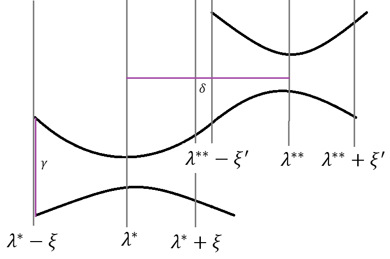
Figure 1: 2 anticrossings in a close vicinity of each other.

We denote the distance between levels $d(\lambda)=x_{m}-x_{n}$, where $x_{m}>x_{n}$, $m$ and $n$ label the levels involved at an anticrossing. Levels are considered to be in an anticrossing when they are in a $\gamma$ neighbourhood of each other about a local minimum denoted by $d(\lambda^{*})=\Delta_{min}$ where $\dot{d}(\lambda^{*})=0$. Expanding $d(\lambda)$ about $\lambda^{*}$ where $\delta\lambda=(\lambda-\lambda^{*})$, we obtain the following (details are provided in Appendix D):

$$\begin{gathered}d(\lambda)=\Delta_{min}+\delta\lambda^{2}\frac{4\beta^{2}}{\Delta_{min}^{3}}\end{gathered}$$ (8)

Let $d(\lambda^{*}+\xi)=\gamma$, then the minimum separation is expressed as $\Delta_{min}=\gamma-\xi^{2}\frac{4\beta^{2}}{\Delta_{min}^{3}}$. Given that levels are within a distance $\gamma$ of each other and $\delta>\frac{1}{2\dot{\lambda}}(\gamma-\frac{4\beta^{2}}{\Delta_{min}^{3}})+\xi^{{}^{\prime}}$, the anticrossings are considered isolated and one can apply the LZ model. Next, we extend this investigation of the impact of noise under these conditions. This enables further understanding of dissipative influences on the properties of level interactions.

V The impacts of noise on the Landau-Zener conditions in the Pechukas-Yukawa formalism

Depending on the nature of the noise, whether the source is longitudinal (with only diagonal elements) or transverse (with only off-diagonal elements), the system behaves differently. Longitudinal contributions result in decoherence in the system whereas transverse noise results in couplings to the environmentPokSin ; Wilson1 . Our analysis could be extended to various types of noise. For concreteness we consider a single composite source of longitudinal noise, $\delta h$ such that $\dot{\delta}h=\epsilon\eta M$. Here, $\eta$ is white noise, a random normal distributed stochastic processKieselev ; PokSin , $M$ represents a general diagonal matrix and $\epsilon$ denotes the noise amplitude. For white noise, which is the formal derivative of a Wiener process, $W(t)$, the expectation is zero and the autocorrelation function is given by:

$$\begin{gathered}\langle\eta_{mn}(\lambda),\eta_{mn}(\lambda^{{}^{\prime}})\rangle=\delta(\lambda-\lambda^{{}^{\prime}})\\ \langle\epsilon\eta_{mn}(\lambda),\epsilon\eta_{mn}(\lambda^{{}^{\prime}})\rangle=\epsilon^{2}\delta(\lambda-\lambda^{{}^{\prime}})\end{gathered}$$ (9)

The correlation time $\tau_{c}=0$.

Noise can break the degeneracy at level crossings, resulting in anticrossings. To ensure the applicability of the LZ model, we reduce the system from $N$ levels to 2. Again, under the assumption that levels outside the anticrossings are far away with weaker coupling interactions we show that the anticrossing is independent of all non-interacting level contributions. The Pechukas-Yukawa model is highly entangled, hence why it is important to verify that the conditions required for the LZ description are met.

Considering the stochastic Pechukas equations regarding the relative angular momenta, $l_{mn}$ described in Eq. (6), we obtain a driftless geometric Brownian motion for $\dot{l}_{mn}$ for levels $m$ and $n$ in an anticrossing. Then, in the region of the anticrossing $l_{mn}(\lambda)=l_{mn}(\lambda^{*}-\xi)e^{-\frac{\sigma^{2}}{2}(\lambda-(\lambda^{*}-\xi))+\sigma W(\lambda)}$, where $\sigma=\frac{\mu\epsilon}{\Delta_{min}}$. The start time of the levels approaching a minimum separation in a $\gamma$ neighbourhood of each other is taken as $(\lambda^{*}-\xi)$ as in Fig. 1, and $\mu$ denotes the difference in the noise components. The expectation of $l_{mn}$, $E(l_{mn})=l_{mn}(\lambda^{*}-\xi)$ and variance, $Var(l_{mn})=|l_{mn}(\lambda^{*}-\xi)|^{2}(e^{\frac{\sigma^{2}}{2}(\lambda-(\lambda^{*}-\xi))}-1)$. Here, $l_{mn}$ is a martignale, where in the long time limit, $l_{mn}\rightarrow 0$ with probability 1. Substituting these to determine the couplings between non-interacting levels we find that $l_{mi}$ and $l_{ni}$ are stochastic terms, where $Re(l_{mi})=0$ and $Re(l_{ni})=0$ with $Im(l_{mi}),Im(l_{ni})$ bound the interval $[-1,1]$. Taking $\delta\lambda$ sufficiently small, these terms are negligible in the anticrossing. Applying this to the acceleration terms, we find that the difference in acceleration terms is also a stochastic term $\frac{4|l_{mn}|^{2}}{\Delta_{min}^{3}}$. Given that $\tau_{LZ}$ is short, the expectation is strongly bounded in a small interval, choosing $\delta\lambda$ sufficiently small, these terms are also negligible therefore linearising the level separations. Details are provided in Appendix C.

In order for the LZ model to hold in the stochastic sense, it is necessary to consider anticrossings in a close vicinity of each other, such that they can be regarded as isolated crossings. The transition time of an anticrossing is changed under the influence of noise. Of particular interest are the influences of noise on the minimum separation. These in turn have an impact on both the probability of transitions and the transition times.

V.1 Isolated Crossings under the effects of noise

Under the influences of noise on the minimum level separation at $\lambda^{*}$, we investigate its impact on the transition time to determine the conditions required to treat 2 nearby anticrossings independently. We consider 2 neighbouring anticrossings with minimum level separations at $\lambda^{*}$ and $\lambda^{**}=\lambda^{*}+\delta$ and transition times $\tau_{LZ}$ and $\tau^{{}^{\prime}}_{LZ}$ respectively as in Fig. 1. The anticrossings are considered isolated given that the respective transition times do not overlap such that $(\lambda^{**}-\xi^{`})-(\lambda^{*}+\xi)>0$. Then, the Landau-Zener transition model is applicable to describe the probabilities of population transitions.

We denote the distance between levels $d(\lambda)=x_{m}-x_{n}$, where $x_{m}>x_{n}$, $m$ and $n$ label the levels involved at an anticrossing. Expanding $d(\lambda)$ about $\lambda^{*}$, where $f(\lambda)=-\frac{\sigma^{2}}{2}(\lambda-(\lambda^{*}-\xi))+\sigma\eta(\lambda-(\lambda^{*}-\xi))$, we obtain the following (details are provided in Appendix E):

$$\begin{gathered}d(\lambda)=\Delta_{min}\\ +\delta\lambda^{2}\left(\frac{4|l_{mn}(\lambda^{*}-\xi)|^{2}}{\Delta_{min}^{3}}e^{2f(\lambda^{*})}+\epsilon\mu\dot{\eta}(\lambda^{*})\right)\end{gathered}$$ (10)

Let $d(\lambda^{*}+\xi)=\gamma$, then one obtains an expression for the minimum separation:

$$\begin{gathered}\Delta_{min}=\gamma-\\ \xi^{2}\left(\frac{4|l_{mn}(\lambda^{*}-\xi)|^{2}}{\Delta_{min}^{3}}e^{2f(\lambda^{*})}+\epsilon\mu\dot{\eta}(\lambda^{*})\right)\end{gathered}$$ (11)

This describes the relationship between the minimum separation and the difference in noise terms, where $\Delta_{min}\geq 0$. These effects on the level separation affect $\tau_{LZ}$ in the same way. When $\mu=0$, $d(\lambda)=\Delta_{min}+\delta\lambda^{2}(\frac{4|l_{mn}(\lambda^{*}-\xi)|^{2}}{\Delta_{min}^{3}}e^{2f(\lambda^{*})})$. Then the conditions for an isolated anticrossing resemble that of the deterministic case.

Using Eq.(11) in the bound for the transition times, one obtains the following bound, dependent of the difference between the noise sources at a single anticrossing (all details provided in Appendix E):

$$\begin{gathered}\eta(\lambda^{*})>\frac{1}{\xi\epsilon\mu}(\gamma-2\dot{\lambda}(\delta-\xi^{`})-\\ \frac{\xi}{\epsilon\mu}\left(\frac{4|l_{mn}(\lambda^{*}-\xi)|^{2}}{\Delta_{min}^{3}}e^{2f(\lambda^{*})}\right).\end{gathered}$$ (12)

Given this bound is satisfied, the 2 anticrossings are independent of each other, as such the LZ model is applicable.

Therefore, we have shown from the analysis of the levels at a level crossing or anticrossing, the conditions the LZ model imposes on the Pechukas-Yukawa, under the influence of noise.

VI Discussion and Conclusions.

We investigated the compatibility of the LZ transition model in the Pechukas-Yukawa formalism. Taking as starting point all the assumptions that form the basis of the LZ model, we explored the conditions they impose on the Pechukas-Yukawa formalism to be applicable. This led to the development of the understanding of level crossings and anticrossings under this setting, identifying various properties of the level interaction. Particularly, we provided a detailed insight on the level repulsions extended to the influence of external noise and its impacts on the minimum separations characterising anticrossings.

The investigation of level repulsions at an anticrossing under the influence of longitudinal noise was not possible without a thorough description of the level dynamics given by the Pechukas-Yukawa formalism. From this, we built on prior works by [Zagoskin, ] and [Wilson1, ], to gain insight on the level interactions beyond the LZ probability. Under this description, one could investigate the differences in scaling properties observed between edge and intermediate state transitions, observed in [Zagoskin, ] and [Wilson1, ]. An attractive development to this investigation would be to apply the LZ transition probability to the Pechukas-Yukawa description of quantum states which could lead to the exploration of quantum phase transitions through the initial conditions of the eigenvalues of a quantum Hamiltonian system. The eigenstate coefficients have been expressed using the Pechukas equations such that one could extend this description to obtain both the occupation dynamics and the coherences of the system, crucial to the development of AQ-this leads us into our future works. An interesting extension to these works would be to consider the effects of different types of noise such as coloured noise and the impacts of transverse components.

Additionally, these results can be used as a a starting point, to gain insight on multistate LZ transitions. The standard LZ model deals only with the 2 interacting levels. Extending to the multistate problem could yield more interesting physics analytics. The Pechukas-Yukawa model concerns an interacting system of $N$ entangled levels. It is highly equipped to consider interacting systems with entangled states. In further works it would be useful to consider the detailed analytics of multiple level interactions and their influence on each other’s dynamics. One could extend this description to determine the impacts of noise using a master equation.

Appendix A: Reducing System Levels Down to 2-Level Crossings

It is shown below that when there is a level crossing, all non-interacting levels are considered far apart. Then, the Pechukas equations can be reduced to only the interacting levels.

Suppose $x_{m}=x_{n}$ are the interacting levels and all other levels are far apart i.e $x_{m}-x_{k}$ and $x_{n}-x_{k}$ large for $k\neq n,m$ and angular moment $l_{mk}l_{kn}$ are small. Then, the quotient is small and so one takes the folllowing approximation

$$\begin{gathered}\dot{l}_{mn}=\sum_{k\neq m,n}{l_{mk}l_{kn}\left(\frac{1}{{(x_{m}-x_{k})}^{2}}-\frac{1}{({x_{k}-x_{n})}^{2}}\right)}\approx 0\\ \end{gathered}$$ (13)

By the definition of the Pechukas equations when $x_{m}=x_{n}$, $l_{mn}=0$ hence $l_{mn}$ stays constantly zero throughout the transition time.

Similarly, the other non-interacting angular momenta can be paired into the following coupled differential equations. All other terms are negligible. These are approximated as follows: for $i\neq m,n$

$$\begin{gathered}\dot{l}_{mi}\approx{l_{mn}l_{ni}\left(\frac{1}{{(x_{m}-x_{n})}^{2}}\right)}\\ \dot{l}_{ni}\approx{l_{nm}l_{mi}\left(\frac{1}{{(x_{n}-x_{m})}^{2}}\right)}\\ \end{gathered}$$ (14)

Applying l’Hopital’s rule on this term twice, we have shown this term tends to 0 as $\lambda\rightarrow\lambda^{*}$ demonstrating the relative angular momenta terms can be reduced to only the interacting levels under this approximation. It follows that the acceleration terms are also independent of all other level interactions, determined by the following:

$$\begin{gathered}\dot{v}_{m}=2\sum_{i\neq n}{\frac{{{|l}_{mi}|}^{2}}{{(x_{m}-x_{i})}^{3}}}+{\frac{{{|l}_{mn}|}^{2}}{{(x_{m}-x_{n})}^{3}}}\\ \dot{v}_{i}=2\sum_{i,j\neq m,n}{\frac{{{|l}_{ij}|}^{2}}{{(x_{i}-x_{j})}^{3}}}+{\frac{{{|l}_{mj}|}^{2}}{{(x_{m}-x_{j})}^{3}}}\\ +{\frac{{{|l}_{nj}|}^{2}}{{(x_{n}-x_{j})}^{3}}}\\ \end{gathered}$$ (15)

Again the same argument holds for $\dot{v}_{n}$ as does $\dot{v}_{m}$. Using the expressions in Eq.(13), $l_{mi}$ is constant hence the terms under the sum in $\dot{v}_{m}$ are negligible. After performing l’Hopital 3 times, the expression ${\frac{{{|l}_{mn}|}^{2}}{{(x_{m}-x_{n})}^{3}}}$ was found to tend to 0 as $\lambda\rightarrow\lambda^{*}$. Expanding about $\lambda^{*}$, level separation is described by $x_{m}-x_{n}=\delta\lambda(v_{m}-v_{n})+\delta\lambda^{2}(\dot{v}_{m}-\dot{v}_{n})+{\cal O}(\delta\lambda^{3})$, where acceleration terms idependently tend to 0 at a level crossing. This linearises level separtions in this region during the Landau-Zener transition. For $v_{m}=v_{n}$, the numerator and denominator in the accelleration terms, identically go to 0, thus one can treat $\dot{v}_{m}$ as constant, such that for small $\delta\lambda$ level separation can be taken as linear. This argument holds identically for $\dot{v}_{n}$. For the $\dot{v}_{i}$ expression, all terms are negligible.

This demonstrates the applicability of the Pechukas-Yukawa formalism to the LZ model as one can indeed reduce and $N$ level system down to 2, neglecting all other interactions.

Appendix B: Reducing $N$ Levels Down to 2-Anticrossings Without Noise

Anticrossings occur when levels approaching each other, reach a local minimum before deflecting away. In such cases, $x_{m}-x_{n}=\Delta_{min}$ and $l_{mn}$ is not neccessarily 0. In the same way, Eq.(13) and Eq.(15) apply. Under the same approximation that all other levels are far away, again $\dot{l}_{mn}=0$ thus $l_{mn}=\beta$ where $\beta$ is a constant. Considering the equations for $l_{mi}$ and $l_{ni}$, the only surviving terms are:

$$\begin{gathered}\dot{l}_{mi}={l_{mn}l_{ni}\left(\frac{1}{{(x_{m}-x_{n})}^{2}}\right)}={l_{ni}\beta\left(\frac{1}{{\Delta_{min}}^{2}}\right)}\\ \dot{l}_{ni}={l_{mn}l_{mi}\left(\frac{1}{{(x_{n}-x_{m})}^{2}}\right)}=-{l_{mi}\beta^{*}\left(\frac{1}{{\Delta_{min}}^{2}}\right)}\end{gathered}$$ (16)

We obtain coupled differential equations. Rewritten as $\left(\begin{matrix}\dot{l}_{mi}\\ \dot{l}_{ni}\end{matrix}\right)=\frac{1}{\Delta_{min}^{2}}\left(\begin{matrix}0&&\beta\\ -\beta^{*}&&0\end{matrix}\right)\left(\begin{matrix}l_{mi}\\ l_{ni}\end{matrix}\right)$. The system is readily solved as:

$$\begin{gathered}l_{mi}=\frac{i\beta}{|\beta|}\frac{1}{2}\left(e^{\frac{i|\beta|}{\Delta_{min}^{2}}}+e^{\frac{-i|\beta|}{\Delta_{min}^{2}}}\right)=\frac{i\beta}{|\beta|}\cos\left(\frac{|\beta|}{\Delta_{min}^{2}}\right)\\ l_{ni}=\frac{-1}{2}(e^{\frac{i|\beta|}{\Delta_{min}^{2}}}-e^{-\frac{i|\beta|}{\Delta_{min}^{2}}})=-i\sin(\frac{|\beta|}{\Delta_{min}^{2}})\end{gathered}$$ (17)

Then about $\lambda^{*}$, the relative angular momenta $l_{mn}$ are constants independent of all other levels. We further showed, $l_{mi}$ and $l_{ni}$ are constants with $Re(l_{mi})=0$ and $Re(l_{ni})=0$ with $Im(l_{mi})$ and $Im(l_{ni})$, bounded between [-1, 1], hence the couplings between the levels involved in an anticrossing and those that are not, are weak . This allows for treating the anticrossing, independent of all other levels. Substituting these results into Eq.(15), $\dot{v}_{i}=0$, the only surviving terms in $\dot{v}_{m}$ and $\dot{v}_{n}$ are constants; $(\dot{v}_{m}-\dot{v}_{n})=\frac{{4|\beta|}^{2}}{{\Delta_{min}}^{3}}$. For sufficiently small $\delta\lambda$, one can linearise the level separations such that level evolutions are reduced to only the interacting levels. Then, it is justifiable in applying the Pechukas-Yukawa formalism to the Landau-Zener model for anticrossings.

Appendix C: Isolated Crossings for a Deterministic Case

We denote level separations as $d(\lambda)=x_{1}-x_{2}$, where $d(\lambda^{*})=\Delta_{min}$. Let $\delta\lambda=\lambda-\lambda^{*}$, then expanding about $\lambda^{*}$, $d(\lambda)=\Delta_{min}+\delta\lambda(v_{1}-v_{2}+\dot{\delta}h_{11}-\dot{\delta}h_{22})+\delta\lambda^{2}(\frac{4\beta^{2}}{\Delta_{min}^{3}}+\ddot{\delta}h_{11}-\ddot{\delta}h_{22})+{\cal O}(\delta\lambda^{3})$. Given that $d(\lambda)$ reaches a local minimum at $\lambda^{*}$, then $v_{1}-v_{2}+\dot{\delta}h_{11}-\dot{\delta}h_{22}=0$.

Take $d(\lambda^{*}+\xi)=\gamma$, such that one could rearrange the equation to obtain:

$$\begin{gathered}\Delta_{min}=\gamma-\xi^{2}\frac{4\beta^{2}}{\Delta_{min}^{3}}\end{gathered}$$ (18)

In order to ensure that anticrossings can be treated independently, $(\lambda^{**}-\xi^{{}^{\prime}})-(\lambda^{*}+\xi)>0$ where $\lambda^{**}=\lambda^{*}+\delta$. Recall $\tau_{LZ}=\frac{\Delta_{min}}{\dot{\lambda}}=2\xi$ for a symmetric anticrossing. Then it is essentially $\tau_{LZ}<2(\delta-\xi^{{}^{\prime}})$. One could rearrange this bound for $\Delta_{min}$,

$$\begin{gathered}\gamma-\xi^{2}\frac{4\beta^{2}}{\Delta_{min}^{3}}<2\dot{\lambda}(\delta-\xi^{{}^{\prime}})\end{gathered}$$ (19)

Given that $\delta>\frac{1}{2\dot{\lambda}}(\gamma-\frac{4\beta^{2}}{\Delta_{min}^{3}}\xi^{2})+\xi^{`}$, the conditions for anticrossings to be treated independently are satisfied.

Appendix D: Reducing $N$ Levels Down to 2-Anticrossings With Noise

When noise is present in a system, level interactions are always non-degenerate occuring with anticrossings. To determine the applicability of the Pechukas-Yukawa formalism under dissiptive influences, it is neccessary to ensure that level interactions in an anticrossing are independent of all other interactions. Again, $x_{m}-x_{n}=\Delta_{min}$ at some $\lambda^{*}$ (denoting the point of minimum separation) and $l_{mn}$ is not neccessarily 0. Similarly to Eq.(13), we have the following for the coupling between levels at an anticrossing.

$$\begin{gathered}\dot{l}_{mn}=\sum_{k\neq m,n}{l_{mk}l_{kn}\left(\frac{1}{{(x_{m}-x_{k})}^{2}}-\frac{1}{({x_{k}-x_{n})}^{2}}\right)}\\ +\frac{(x_{m}-x_{n})(l_{mk}\dot{\delta}h_{km}-\dot{\delta}h_{mk}l_{kn})}{(x_{m}-x_{k})(x_{n}-x_{k})}+\\ \dot{\delta}h_{mn}(v_{m}-v_{n})+\frac{l_{mn}(\dot{\delta}h_{mm}-\dot{\delta}h_{nn})}{(x_{m}-x_{n})}\\ \end{gathered}$$ (20)

We consider a single source of composite longitudinal noise. Again, we assume all non-interacting levels are far away with weak couplings such that $l_{mk}l_{kn}$ are small for $k\neq n,m$. This simplifies the relative angular momena dynamics to the following:

$$\begin{gathered}\dot{l}_{mn}\approx\frac{l_{mn}(\dot{\delta}h_{mm}-\dot{\delta}h_{nn})}{(x_{m}-x_{n})}\\ \approx\frac{l_{mn}}{\Delta_{min}}\epsilon\mu\eta\end{gathered}$$ (21)

where $\epsilon$ denotes the noise amplitude, $\mu$ is a constant giving the difference between the noise components and $\eta$ represents a white noise stochasti term. Let $\sigma=\frac{\epsilon\mu}{\Delta_{min}}$. We consider separately, real and imaginary components. In each component, we observe a driftless geometric Brownian motion.

$$\begin{gathered}\dot{R}e(l_{mn})=\sigma Re(l_{mn})\eta\\ \dot{I}m(l_{mn})=\sigma Im(l_{mn})\eta\\ \end{gathered}$$ (22)

Using the Euler-Maruyama method to solve these stochastic differential equations, we rewrite the expression for $Re(l_{mn})$ as $dRe(l_{mn})=\sigma Re(l_{mn})dW$. Integrating these terms, where we zero out noise at $\lambda^{*}-\xi$, we obtain the following:

$$\begin{gathered}\int_{\lambda^{*}-\xi}^{\lambda}\frac{dRe(l_{mn})}{l_{mn}}=\sigma dW\\ \end{gathered}$$ (23)

Applying Ito’s formula,

$$\begin{gathered}d(Ln(Re(l_{mn})))=\frac{dRe(l_{mn})}{l_{mn}}-\frac{1}{2}\frac{1}{Re(l_{mn})^{2}}dRe(l_{mn})dRe(l_{mn})\\ \end{gathered}$$ (24)

where $dRe(l_{mn})dRe(l_{mn})$ is the quadratic variation of the stochastic differential equation such that $dRe(l_{mn})dRe(l_{mn})=\sigma^{2}Re(l_{mn})^{2}d\lambda$. Substituting this into the integral, we have:

$$\begin{gathered}\int_{\lambda^{*}-\xi}^{\lambda}d(Ln(Re(l_{mn})))+\frac{\sigma^{2}}{2}=\sigma dW\\ \end{gathered}$$ (25)

Then,

$$\begin{gathered}Ln\left(\frac{Re(l_{mn}(\lambda))}{Re(l_{mn}(\lambda^{*}-\xi))}\right)\\ =-\frac{1}{2}\sigma^{2}(\lambda-(\lambda^{*}-\xi))+\sigma W(\lambda)\end{gathered}$$ (26)

Exponentiating the result, we find that $Re(l_{mn}(\lambda))=Re(l_{mn}(\lambda^{*}-\xi))e^{-\frac{\sigma^{2}}{2}(\lambda-(\lambda^{*}-\xi))+\sigma W(\lambda)}$. Using the same method to solve for the imaginary components, we have $Im(l_{mn}(\lambda))=Im(l_{mn}(\lambda^{*}-\xi))e^{-\frac{\sigma^{2}}{2}(\lambda-(\lambda^{*}-\xi))+\sigma W(\lambda)}$. Combining these terms, $l_{mn}(\lambda)=l_{mn}(\lambda^{*}-\xi)e^{-\frac{\sigma^{2}}{2}(\lambda-(\lambda^{*}-\xi))+\sigma\eta(\lambda)}$ in the region of the transition time. This term has expectation, $E(l_{mn})=l_{mn}(\lambda^{*}-\xi)$ and variance $Var(l_{mn})=|l_{mn}(\lambda^{*}-\xi)|^{2}(e^{\frac{\sigma^{2}}{2}(\lambda-(\lambda^{*}-\xi))}-1)$. Here, $(\lambda^{*}-\xi)$ represents the start time of levels approaching a minimum separation in a $\gamma$ neighbourhood of each other. This describes $l_{mn}$ as a martingale where for $\lambda\rightarrow\infty,l_{mn}\rightarrow 0$ with probability 1, which follows from the law of iterative logarithm.

The equations for $l_{mi}$ are given by the following:

$$\begin{gathered}\dot{l}_{mi}=\sum_{k\neq m,i;i\neq n}{l_{mk}l_{ki}\left(\frac{1}{{(x_{m}-x_{k})}^{2}}-\frac{1}{({x_{k}-x_{i})}^{2}}\right)}\\ +\frac{(x_{m}-x_{i})(l_{mk}\dot{\delta}h_{km}-\dot{\delta}h_{mk}l_{ki})}{(x_{m}-x_{k})(x_{i}-x_{k})}+\\ \dot{\delta}h_{mn}(v_{m}-v_{i})+\frac{l_{mi}(\delta h_{mm}-\delta h_{ii})}{(x_{m}-x_{i})}+\\ {l_{mk}l_{kn}\left(\frac{1}{{(x_{m}-x_{k})}^{2}}-\frac{1}{({x_{k}-x_{n})}^{2}}\right)}\\ +\frac{(x_{m}-x_{n})(l_{mk}\dot{\delta}h_{km}-\dot{\delta}h_{mk}l_{kn})}{(x_{m}-x_{k})(x_{n}-x_{k})}+\\ \dot{\delta}h_{mn}(v_{m}-v_{n})+\frac{l_{mn}(\delta h_{mm}-\delta h_{nn})}{(x_{m}-x_{n})}\\ \end{gathered}$$ (27)

The equations are identical for $l_{ni}$. Again, under the same assumptions used for $\dot{l}_{mn}$, we obtain the following pairs of coupled differential equations:

$$\begin{gathered}\dot{l}_{mi}\approx l_{mn}l_{ni}\left(\frac{1}{{(x_{m}-x_{n})}^{2}}\right)=l_{mn}l_{ni}\left(\frac{1}{{\Delta_{min}}^{2}}\right)\\ \dot{l}_{ni}\approx l_{nm}l_{mi}\left(\frac{1}{{(x_{n}-x_{m})}^{2}}\right)=-l_{mn}^{*}l_{mi}\left(\frac{1}{{\Delta_{min}}^{2}}\right)\\ \end{gathered}$$ (28)

Taking a matrix of ordinary differential equations, we have

$$\begin{gathered}\left(\begin{matrix}\dot{l}_{mi}\\ \dot{l}_{ni}\end{matrix}\right)=\frac{f(\lambda)}{\Delta_{min}^{2}}\left(\begin{matrix}0&&l_{mn}(\lambda^{*}-\xi)\\ -l_{mn}^{*}(\lambda^{*}-\xi)&&0\end{matrix}\right)\left(\begin{matrix}l_{mi}\\ l_{ni}\end{matrix}\right)\end{gathered}$$ (29)

Where $f(\lambda)=e^{\frac{\sigma^{2}}{2}(\lambda-(\lambda^{*}-\xi))+\sigma\eta(\lambda)}$, capturing the stochastic element. Diagonalising the matrix and changing bases to the eigenvectors, we can simply integrate the decoupled set of equations. We obtain the following:

$$\begin{gathered}l_{mi}=\frac{il_{mn}}{2|l_{mn}|}\left(e^{i\frac{f(\lambda)}{\Delta_{min}^{2}}|l_{mn}|}+e^{-i\frac{f(\lambda)}{\Delta_{min}^{2}}|l_{mn}|}\right)\\ =\frac{il_{mn}}{|l_{mn}|}cos\left(\frac{f(\lambda)}{\Delta_{min}^{2}}|l_{mn}|\right)\\ l_{ni}=-\frac{1}{2}\left(e^{i\frac{f(\lambda)}{\Delta_{min}^{2}}|l_{mn}|}-e^{-i\frac{f(\lambda)}{\Delta_{min}^{2}}|l_{mn}|}\right)\\ =-isin\left(\frac{f(\lambda)}{\Delta_{min}^{2}}|l_{mn}|\right)\\ \end{gathered}$$ (30)

Then, $l_{mi}$ and $l_{ni}$ are stochastic terms, where $Re(l_{mi})=0$ and $Re(l_{ni})=0$ with $Im(l_{mi}),Im(l_{ni})$ bounded in the interval $[-1,1]$. Taking $\delta\lambda$ sufficiently small, these terms are negligible in the anticrossing. Applying these relative angular momenta formulae to the acceleration terms (again modelling the noise to be a longitudinal composite source) we have the following:

$$\begin{gathered}\dot{v}_{m}=2\sum_{i\neq n}{\frac{{{|l}_{mi}|}^{2}}{{(x_{m}-x_{i})}^{3}}}+\frac{2\dot{\delta}h_{mi}Re(l_{mi})}{{(x_{m}-x_{i})}^{2}}\\ +{\frac{{{|l}_{mn}|}^{2}}{{(x_{m}-x_{n})}^{3}}}+\frac{2\dot{\delta}h_{mn}Re(l_{mn})}{{(x_{m}-x_{n})}^{2}}\\ \dot{v}_{i}=2\sum_{i,j\neq m,n}{\frac{{{|l}_{ij}|}^{2}}{{(x_{i}-x_{j})}^{3}}}+\frac{2\dot{\delta}h_{mi}Re(l_{mi})}{{(x_{m}-x_{i})}^{2}}\\ +{\frac{{{|l}_{mj}|}^{2}}{{(x_{m}-x_{j})}^{3}}}+\frac{2\dot{\delta}h_{mi}Re(l_{mi})}{{(x_{m}-x_{i})}^{2}}\\ +{\frac{{{|l}_{nj}|}^{2}}{{(x_{n}-x_{j})}^{3}}}+\frac{2\dot{\delta}h_{mi}Re(l_{mi})}{{(x_{m}-x_{i})}^{2}}\\ \end{gathered}$$ (31)

All terms are negligible for $v_{i}$ under the approximation on the level separation in this regions is negligible.

For the difference between $\dot{v}_{m}$ and $\dot{v}_{n}$, all terms under the sum are negligible except for ${\frac{4{|l_{mn}|}^{2}}{{\Delta_{min}}^{3}}}$, which is independent of all other levels. To determine the effects of the stochastic terms on the difference between accelerations, we consider the expectation during $\tau_{LZ}$. The expectation of $|l_{mn}|^{2}$, is given by:

$$\begin{gathered}|l_{mn}|^{2}=Re(l_{mn})^{2}+Im(l_{mn})^{2}\\ E|l_{mn}|^{2}=E(Re(l_{mn})^{2})+E(Im(l_{mn})^{2})\\ =Var(Re(l_{mn}))+Var(Im(l_{mn}))\\ +E^{2}(Re(l_{mn}))+E^{2}(Im(l_{mn}))\\ =|l_{mn}(\lambda^{*}+\xi)|^{2}e^{\frac{\sigma^{2}}{2}(\lambda-(\lambda^{*}-\xi))}\end{gathered}$$ (32)

Then the expectation of the difference between the acceleration terms are given by $\frac{4|l_{mn}(\lambda^{*}+\xi)|^{2}}{\Delta_{min}^{3}}e^{\frac{\sigma^{2}}{2}(\lambda-(\lambda^{*}-\xi))}$. These dynamics are bounded between $[\frac{4|l_{mn}(\lambda^{*}+\xi)|^{2}}{\Delta_{min}^{3}},\frac{4|l_{mn}(\lambda^{*}+\xi)|^{2}}{\Delta_{min}^{3}}e^{\xi\sigma^{2}}]$ where $\lambda\in[\lambda^{*}-\xi,\lambda^{*}+\xi]$. For $\tau_{LZ}$ being short time durations, this motion is under stricter bounds, near-constant. In taking $\delta\lambda$ small enough, the difference in accelaration terms are negligible, linearising the level separations. Then it is observed that indeed the Pechukas-Yukawa formalism under the influence of noise is applicable to the LZ model, reducing the system from N levels to 2.

Appendix E: Isolated Crossings for a Stochastic Case

Under the influences of noise, the level separations expanded about $\lambda^{*}$ are given by $d(\lambda)=\Delta_{min}+\delta\lambda^{2}\left(\frac{4|l_{mn}(\lambda^{*}-\xi)|^{2}}{\Delta_{min}^{3}}e^{2f(\lambda^{*})}+\epsilon\mu\dot{\eta}(\lambda^{*})\right)$. Let us denote the level separation at the final instant by $d(\lambda^{*}+\xi)=\gamma$, then one can once again rearrange for $\Delta_{min}$:

$$\begin{gathered}\Delta_{min}=\gamma-\\ \xi^{2}\left(\frac{4|l_{mn}(\lambda^{*}-\xi)|^{2}}{\Delta_{min}^{3}}e^{2f(\lambda^{*})}+\epsilon\mu\dot{\eta}(\lambda^{*})\right)\end{gathered}$$ (33)

Again, for symmetric anticrossings, one obtains the following bound:

$$\begin{gathered}\gamma-\xi^{2}\left(\frac{4|l_{mn}(\lambda^{*}-\xi)|^{2}}{\Delta_{min}^{3}}e^{2f(\lambda^{*})}+\epsilon\mu\dot{\eta}(\lambda^{*})\right)<2\dot{\lambda}(\delta-\xi^{`})\end{gathered}$$ (34)

Integrating over the transition time on both sides and rearranging for $\eta(\lambda^{*})$, we reduce the bound to the following:

$$\begin{gathered}\eta(\lambda^{*})>\frac{1}{\xi\epsilon\mu}(\gamma-2\dot{\lambda}(\delta-\xi^{`})-\\ \frac{\xi}{\epsilon\mu}\left(\frac{4|l_{mn}(\lambda^{*}-\xi)|^{2}}{\Delta_{min}^{3}}e^{2f(\lambda^{*})}\right)\\ \end{gathered}$$ (35)

This provides a bound on the system, accounting for noise. Given the noise at $\lambda^{*}$ satisfies this bound, the conditions for level crossings to be treated independently hold. Then, the LZ model is applicable. These equations detail a system with a single composite source of longitudinal noise and its impact on the probability of isolated level crossings. These can be explored for various cases under different types of noise.

References

- (1) A.M. Zagoskin, E. Il’ichev, M. Grajcar, J.J. Betouras, and F. Nori, Front. Physics 2, 33 (2014).
- (2) R Requist, J Schliemann, AG Abanov, D Loss, Phy. Rev. B 71, 115315 (2005).
- (3) E. Fahri et al., Science 292, 472 (2001).
- (4) A. M. Childs, E. Farhi, J. Preskill, Phys. Rev. A 65, 012322 (2001).
- (5) M. Sarovar, K. C. Young, New Journal of Physics, 15 125032 (2013).
- (6) R. Di Candia, B. Mejia, H. Castillo, J. S. Pedernales, J. Casanova and E. Solano, Phys. Rev. Lett. 111, 240502 (2013).
- (7) P. Pechukas, Phys. Rev. Lett. 51, 943 (1983)
- (8) T. Yukawa and T. Ishikawa, Prog. Theor. Phys. Suppl. 98, 157 (1989).
- (9) G. Schaller, S. Mostame, R. Schutzhold, Phys. Rev. A 73, 062307 (2006).
- (10) F. Haake, Quantum Signitures of Chaos, Ch. 6 (Springer, Berlin, 2001).
- (11) M. A. Qureshi, J. Zhong, J. J. Betouras, A. M. Zagoskin, Phys. Rev. A 95, 032126 (2017).
- (12) R. Requist, Phys. Rev. A 86 (2), 022117 (2012).
- (13) A. M. Zagoskin, S. Savel’ev and F. Nori, Phys. Rev. Lett. 98, 120503 (2007).
- (14) R. Barends, A. Shabani, L. Lamata, J. Kelly et al, Nature 534, 17658 (2016).
- (15) J. Huyghebaert and H. De Raedt, J. Phys. A 23, 5777-5793 (1990).
- (16) R. D. Wilson, A. M. Zagoskin and S. Savel’ev, Phys. Rev. A 82, 052328 (2010).
- (17) M. A. Qureshi, J. Zhong, Z. Qureshi, P. Mason, J. J. Betouras, A. M. Zagoskin, Phys. Rev. A 97, 032117 (2018).
- (18) Y. Kayanuma, H. Nakayama, Phys. Rev. B 57, 13099 (1998)
- (19) V. L. Pokrovsky, N. A. Sinitsyn, Phys. Rev. B 67, 144303 (2003)
- (20) P. Cejnar, J. Jolie, Prog. Part. Nucl. Phys. 62, 210-256 (2009)
- (21) A. J. Leggett, S. Chakravarty, A. T. Dorsey, M. P. A. Fisher, A. Garg and W. Zwerger, Rev. Mod. Phys. 59, 1 (1987)
- (22) T. Yukawa, Phys. Rev. Lett. 54, 1883 (1985).
- (23) R. D. Wilson, A. M. Zagoskin, S. Savel’ev, M. J. Everitt and F. Nori, Phys. Rev. A 86, 052306 (2012).
- (24) N. V. Vitanov and B. M. Garraway, Phys. Rev. A 53, 4288 (1996)
- (25) J. R. Rubbmark, M. M. Kash, M. G. Littman and D. Kleppner, Phys. Rev. A 23, (6) 3107 (1981)
- (26) M. Wilkinson, J. Phys. A: Math. Gen. 21, 4021-4037 (1988)
- (27) M. Wilkinson, J. Phys. A: Math. Gen. 22, 2795-2805 (1989)
- (28) J. Zakrzewski, D. Delande, M. Kus, Phys. Rev. E 47, (3) 1665 (1993)
- (29) M. H. S. Amin, D. V. Averin and J. A. Nesteroff, Phys. Rev. A 79, 022107 (2009)
- (30) M. B. Kenmoe, H. N. Phien, M. N. Kiselev and L. C. Fai, Phys. Rev. B 87, 224301 (2013)
- (31) Z. X. Luo and M. E. Raikh, Phys. Rev. B 95, 064305 (2017)
- (32) G. E. Astrakharchik, D. M. Gangardt, Yu. E. Lozovik, I. A. Sorokin, Phys. Rev. E 74, 021105 (2006)