Principal Component Analysis with Tensor Train Subspace

Abstract

Tensor train is a hierarchical tensor network structure that helps alleviate the curse of dimensionality by parameterizing large-scale multidimensional data via a set of network of low-rank tensors. Associated with such a construction is a notion of Tensor Train subspace and in this paper we propose a TT-PCA algorithm for estimating this structured subspace from the given data. By maintaining low rank tensor structure, TT-PCA is more robust to noise comparing with PCA or Tucker-PCA. This is borne out numerically by testing the proposed approach on the Extended YaleFace Dataset B.

I Introduction

Robust feature extraction and dimensionality reduction are among the most fundamental problems in machine learning and computer vision. Assuming that the data is embedded in a low dimensional subspace, popular and effective methods for feature extraction and dimensionality reduction are the Principal Component Analysis (PCA) [11, 3], and the Laplacian eigenmaps [2]. In this paper we consider structured subspace models, namely tensor subspaces to further refine these subspace based approaches, with significant gains on processing and handling multidimensional data.

Most of the real-world data is multidimensional, i.e. it is a function of several independent variables, and typically represented by a multidimensional array of numbers. These arrays are often referred to as tensors, terminology borrowed from multilinear algebra [7]. For example, a color image can be considered as a third-order tensor, two of the dimensions (rows and columns) being spatial, and the third being spectral (color), while a color video sequence can be considered as an four-order tensor, time being the fourth dimension besides spatial and spectral.

A very popular tensor representation format namely the Tucker format has shown to be useful for a variety of applications [7, 8, 13, 18, 23]. However, for large tensors, Tucker representation can still be exponential in storage requirements. In [10] it was shown that hierarchical Tucker representation, and in particular Tensor Train (TT) representation can alleviate this problem. Nevertheless, the statistical and computational tradeoffs of such reduced complexity formats, such as the TT, have not been studied so far.

In this paper, we begin by showing that TT decompositions are associated with a structured subspace model, namely the Tensor Train subspace. Based on this model, the problem of finding the Tensor Train subspace and the representation of the data is formulated as an extension of the Tucker and traditional PCA based technique. An algorithm to solve this non-convex problem is provided, and is referred to as TT-PCA. We show that if the data admits a TT representation, then TT-PCA significantly reduces storage and complexity as compared to the standard PCA and the Tucker-PCA (T-PCA). We use TT-PCA for classification on Extended YaleFace Dataset B [9, 12], where different images of 38 humans are classified. We see that TT-PCA is able to exploit the structure better than the standard PCA and the T-PCA approaches and achieves the lowest classification error at a lower amount of compressed data dimension.

The rest of the paper is organized as follows. The technical notations and definitions are introduced in Section II. The tensor train subspace (TT-subspace) model is described in Section III, and TT-PCA algorithm is proposed in Section IV. Section V provides the numerical results for the proposed algorithms on Yale Face and MNIST databases. Finally, Section VI concludes the paper.

II Notations and Preliminaries

In this section, we introduce the notations that will be extensively used in this paper. Vectors and matrices are represented by bold face lower letters (e.g. ${\bf x}$) and bold face capital letters (e.g. ${\bf X}$), respectively. An identity matrix of $r$ rows is denoted as ${\bf I}^{r}$. Transpose of matrix ${\bf X}$ is denoted by ${\bf X}^{T}$. An $n^{\text{th}}$ order tensor is denoted by calligraphic letter ${\mathscr{X}}\in\mathbb{R}^{I_{1}\times I_{2}\times...\times I_{n}}$, where $I_{i:i=1,2,...,n}$ is the dimension along the $i^{\text{th}}$ mode. An entry inside a tensor $\mathscr{X}$ is represented as $\mathscr{X}(i_{1},i_{2},\cdots,i_{n})$, where $i_{k:k=1,2,..,n}$ is the location index along the $k^{\text{th}}$ mode. A colon is applied to represent all the elements of a mode in a tensor, e.g. $\mathscr{X}(:,i_{2},\cdots,i_{n})$ represents the fiber along mode $1$ and $\mathscr{X}[:,:,i_{3},i_{4},\cdots,i_{n}]$ represents the slice along mode $1$ and mode $2$ and so forth. ${\bf V}(\cdot)$ is a tensor vectorization operator such that $\mathscr{X}\in\mathbb{R}^{I_{1}\times\cdots\times I_{n}}$ maps to a vector ${\bf V}({\mathscr{X}})\in\mathbb{R}^{I_{1}\cdots I_{n}}$.

Under tucker format [6], any entry insider a tensor is represented by the Tucker Decomposition

$$\begin{split}&\mathscr{X}(i_{1},\cdots,i_{n})\\ =&\sum_{j_{1}=1}^{r_{1}}\cdots\sum_{j_{n}=1}^{r_{n}}\mathscr{C}(j_{1},\cdots,j_{n}){\bf U}_{1}(i_{1},j_{1})\cdots{\bf U}_{n}(i_{n},j_{n}),\end{split}$$

where $\mathscr{C}\in\mathbb{R}^{r_{1}\times\cdots\times r_{n}}$ is the core tensor and ${\bf U}_{i}\in\mathbb{R}^{I_{i}\times r_{i}}$ are the set of orthonormal linear transformation that defines the tucker structure. The Tucker-Rank is denoted by the vector of ranks $(r_{1},\cdots,r_{n})$ in the Tucker Decomposition. The multilinear subspace is defined by the span of a given set of core tensors after the set of linear transformation given by ${\bf U}_{i}$. In this paper, we refer the method to recover the multilinear subspace, or the Tucker Subspace, as Tucker PCA (T-PCA).

Tensor train decomposition [16, 10] is a tensor factorization method that any elements inside a tensor $\mathscr{X}\in\mathbb{R}^{I_{1}\times\cdots\times I_{n}}$, denoted as $\mathscr{X}(i_{1},i_{2},\cdots,i_{n})$, is represented by

$$\begin{split}&\mathscr{X}(i_{1},\cdots,i_{n})\\ &={\bf U}_{1}(i_{1},:)\mathscr{U}_{2}(:,i_{2},:)\cdots\mathscr{U}_{n-1}(:,i_{n-1},:){\bf U}_{n}(:,i_{n}),\end{split}$$

where ${\bf U}_{1}\in\mathbb{R}^{I_{1}\times r_{1}}$, ${\bf U}_{n}\in\mathbb{R}^{r_{n-1}\times I_{n}}$ are the boundary matrices and $\mathscr{U}_{i}\in\mathbb{R}^{r_{i-1}\times I_{i}\times r_{i}},i=2,\cdots,n-1$ are middle decomposed tensors. Without loss of generality, we can define ${\mathscr{U}}_{1}\in\mathbb{R}^{1\times I_{1}\times r_{1}}$ as the tensor representing ${\bf U}_{1}$, and $\mathscr{U}_{n}\in\mathbb{R}^{r_{n-1}\times I_{n}\times 1}$ representing ${\bf U}_{n}$. The TT-Rank of a tensor is denoted by the vector of ranks $(r_{1},\cdots,r_{n-1})$ in the tensor train decomposition. We let $r_{0}=1$. We note that the representation of a tensor as the product of tensors is called the Matrix Product State Structure, and the different ${\mathscr{U}}_{i}$ are called Matrix Product States (MPS)[17].

We next define the mode-$i$ unfolding of a tensor as follows.

Definition 1.

(Mode-$i$ unfolding [5]) Let $\mathscr{X}\in\mathbb{R}^{I_{1}\times\cdots\times I_{n}}$ be a $n$-mode tensor. Mode-$i$ unfolding of $\mathscr{X}$, denoted as $\mathscr{X}_{[i]}$, matrized the tensor $\mathscr{X}$ by putting the $i^{\text{th}}$ mode in the matrix rows and remaining modes with the original order in the columns such that

$$\mathscr{X}_{[i]}\in\mathbb{R}^{I_{i}\times(I_{1}\cdots I_{i-1}I_{i+1}\cdots I_{n})}.$$ (1)

Next, we define the notion of left-unfolding for third order tensors.

Definition 2.

(Left Unfolding [10]) Let $\mathscr{X}\in\mathbb{R}^{r_{i-1}\times I_{i}\times r_{i}}$ be a third order tensor, the left unfolding is the matrix obtained by taking the first two modes indices as rows indices and the third mode indices as column indices such that ${\bf L}(\mathscr{X})\in\mathbb{R}^{(r_{i-1}I_{i})\times r_{i}}$, and is given as ${\bf L}(\mathscr{X})=(\mathscr{X}_{[3]})^{T}$.

(Left Refolding) Left refolding operator ${\bf L}^{-1}$ is the reverse operator of left unfolding ${\bf L}$, which reshapes a $\mathbb{R}^{(r_{i-1}I_{i})\times r_{i}}$ matrix to a $\mathbb{R}^{r_{i-1}\times I_{i}\times r_{i}}$ tensor.

Similar to left unfolding and refolding, right unfolding is ${\bf R}(\mathscr{X})=\mathscr{X}_{[1]}\in\mathbb{R}^{r_{i-1}\times(I_{i}r_{i})}$.

Definition 3.

(Tensor Connect Product [20]) Let $\mathscr{U}_{i}\in\mathbb{R}^{r_{i-1}\times I_{i}\times r_{i}},i=1,\cdots,n$ be $n$ third order tensors. The tensor connect product $\mathscr{U}_{1}\cdots\mathscr{U}_{n}$ is defined as

$$\mathscr{U}=\mathscr{U}_{1}\cdots\mathscr{U}_{n}\in\mathbb{R}^{r_{0}\times(I_{1}\cdots I_{n})\times r_{n}},\vspace{-.1in}$$ (2)

where for any two adjacent third-order tensor, the tensor connect product satisfies

$$\begin{split}\mathscr{U}_{j}\mathscr{U}_{j+1}&\in\mathbb{R}^{r_{j-1}\times(I_{j}I_{j+1})\times r_{j+1}}\\ &={\bf L}^{-1}\left({\bf I}^{(I_{j+1})}\otimes{\bf L}(\mathscr{U}_{j})\times{\bf L}(\mathscr{U}_{j+1})\right).\end{split}\vspace{-.1in}$$ (3)

Tensor connect product is the tensor product for third order tensors, and matrix product for second order tensors (matrices).

III Tensor Train Subspace (TTS)

A tensor train subspace, ${\bf S_{\text{TT}}}\subseteq\mathbb{R}^{I_{1}\cdots I_{n}}$, is defined as the span of a matrix that is generated by the left unfolding of a tensor, such that

$$\begin{split}{\bf S_{\text{TT}}}&\mathrel{\ensurestackMath{\stackon[1pt]{=}{\scriptstyle\Delta}}}\text{span}({\bf L}(\mathscr{U}_{1}\mathscr{U}_{2}...\mathscr{U}_{n}))\\ &=\{{\bf L}(\mathscr{U}_{1}\mathscr{U}_{2}...\mathscr{U}_{n}){\bf a}|\forall{{\bf a}\in\mathbb{R}^{r_{n}}}\}.\end{split}$$ (4)

We note that a tensor subspace is determined by $\mathscr{U}_{1},\mathscr{U}_{2},\cdots,\mathscr{U}_{n}$, where $\mathscr{U}_{i}\in\mathbb{R}^{r_{i-1}\times I_{i}\times r_{i}}$, $r_{0}=1$ [21]. In a special case when $n=1$, the proposed tensor train subspace is reduced to the linear subspace model under matrix case.

The next result shows that for the given $\mathscr{U}_{1},\mathscr{U}_{2},\cdots,\mathscr{U}_{n}$, ${\bf S_{\text{TT}}}$ is a subspace.

Lemma 1.

(Subspace Property [21]) ${\bf S_{\text{TT}}}$ is a subspace of $\mathbb{R}^{I_{1}\cdots I_{n}}$ for given $\mathscr{U}_{1},\mathscr{U}_{2},\cdots,\mathscr{U}_{n}$.

We next give some properties of the TT decomposition that will be used in this paper.

Lemma 2.

(Left-Orthogonality Property [10, Theorem 3.1]) For any tensor $\mathscr{X}$ of TT-rank ${\mathbf{r}}$, the TT decomposition can be chosen such that ${\bf L}(\mathscr{U}_{i})$ are left-orthogonal for all $i=1,\cdots n$, or ${\bf L}(\mathscr{U}_{i})^{T}{\bf L}(\mathscr{U}_{i})={\bf I}_{r_{i}}\in\mathbb{R}^{r_{i}\times r_{i}}$.

We next show that if ${\bf L}(\mathscr{U}_{i})$ is left-orthogonal for all $i=1,\cdots,n$, then ${\bf L}(\mathscr{U}_{1}\cdots\mathscr{U}_{n})$ is left-orthogonal.

Lemma 3.

(Left-Orthogonality of Tensor Connect Product [21]) If ${\bf L}(\mathscr{U}_{i})$ is left-orthogonal for all $i=1,\cdots,n$, then ${\bf L}(\mathscr{U}_{1}\cdots\mathscr{U}_{j})$ is left-orthogonal for all $1\leq j\leq n$.

Thus, we can without loss of generality, assume that ${\bf L}(\mathscr{U}_{i})$ are left-orthogonal for all $i$. Then, the projection of a data point ${\bf y}\in\mathbb{R}^{r_{n}}$ on the subspace ${\bf S_{\text{TT}}}=\text{span}({\bf L}(\mathscr{U}_{1}\mathscr{U}_{2}...\mathscr{U}_{n}))$ is given by ${\bf L}(\mathscr{U}_{1}\cdots\mathscr{U}_{n})^{T}{\bf y}$.

IV Tensor Train PCA

Given a set of tensor data $\mathscr{X}_{i}\in\mathbb{R}^{I_{1}\times\cdots\times I_{n}}$, $i=1,\cdots,N$, we intend to find $r_{n}$ principal vectors that convert a set of observations of possibly correlated variables into a set of values of linearly uncorrelated variables. The $r_{n}$ principal vectors can be stacked as a matrix ${\bf L}(\mathscr{U}_{1}\mathscr{U}_{2}\cdots\mathscr{U}_{n})\in\mathbb{R}^{I_{1}\cdots I_{n}\times r_{n}}$ such that $\mathscr{U}_{i}\in\mathbb{R}^{r_{i-1}\times I_{i}\times\times r_{i}}$, with $r_{0}=1$. The objective of Tensor Train PCA (TT-PCA) is to find such $\mathscr{U}_{1},\mathscr{U}_{2},\cdots,\mathscr{U}_{n}$ such that the distance of the points from the TTS formed by $\mathscr{U}_{1},\mathscr{U}_{2},\cdots,\mathscr{U}_{n}$ is minimized. We note that for $n=1$, this is the same objective as that for standard PCA [19].

Given $N$ data points $\mathscr{X}_{i}\in\mathbb{R}^{I_{1}\times\cdots\times I_{n}}$, $i=1,\cdots,N$, let ${\bf D}\in\mathbb{R}^{I_{1}\cdots I_{n}\times N}$ be the matrix that concatenates the $N$ vectorizations such that the $i^{\text{th}}$ column of ${\bf D}$ is ${\bf V}({\mathscr{X}}_{i})$. The goal then is to find $\mathscr{U}_{1},\mathscr{U}_{2},\cdots,\mathscr{U}_{n}$ such that the distance of points from the subspace is minimized. More formally, we wish to solve the following problem,

$$\min_{\mathscr{U}_{i},i=1,\cdots,n,{\bf A}}\|{\bf L}(\mathscr{U}_{1}\cdots\mathscr{U}_{n}){\bf A}-{\bf D}\|_{F}^{2}.$$ (5)

IV-A Algorithm

This optimization problem in (5) is a non-convex problem. We however note that the problem is convex w.r.t. each of the variables ($\mathscr{U}_{i},i=1,\cdots,n,{\bf A}$) when the rest are fixed. Thus, one approach to solve the problem is to alternatively minimize over the variables when the rest are fixed.

In this paper, we propose an alternate approach that is based on successive SVD-algorithm for computing TT Decomposition in [10]. The algorithm steps are given in Algorithm 1. The algorithm steps assume that rank vector is not known, and estimates the ranks based on thresholding singular values. However, if the ranks are known, the threshold will be at the $r_{i}$ number of singular values rather than at $\tau$ fraction of the maximum singular value. The proposed algorithm goes from left to right and find the different $\mathscr{U}_{i}$s. We note that this algorithm extends computing TT Decomposition in [10] by thresholding over the singular values, which tries to find the low rank approximation since the data is not exactly low rank. Such approaches for thresholding singular values for data approximation to low rank have been widely used for matrices [4, 8].

The advantage of the approach include the following: (i) There are no iterations like in Alternating Minimization based approach, and the complexity is low. (ii) The obtained ${\bf L}(\mathscr{U}_{i})$ is left-orthogonal for all $i=1,\cdots,N$. Due to this property, we have by Lemma 3 that ${\bf L}(\mathscr{U}_{1}\cdots\mathscr{U}_{n})$ is left-orthogonal. Thus, the projection of a data point ${\mathscr{D}}\in\mathbb{R}^{I_{1}\times\cdots\times I_{n}}$ onto the TT subspace formed is $({\bf L}(\mathscr{U}_{1}\cdots\mathscr{U}_{n}))^{T}{\bf V}(\mathscr{D})$ .

Algorithm 1 Tensor Train Principle Component Analysis (TT-PCA) Algorithm

1:$N$ tensors $\mathscr{X}_{i}\in\mathbb{R}^{I_{1}\times I_{2}\times\cdots\times I_{n}}$, $i=1,\cdots,N$, threshold parameter $\tau$

2:Decomposition for tensor train subspace $\mathscr{U}_{1},\mathscr{U}_{2},\cdots,\mathscr{U}_{n}$ and the representation ${\bf A}$

3:Form $\mathscr{Y}$ as an order $n+1$ tensor s.t. $\mathscr{Y}\in\mathbb{R}^{I_{1}\times I_{2}\times\cdots\times I_{n}\times N}$, which is formed by concatenating all data points $\mathscr{X}_{i}$ in the last mode.

4:Set ${\bf X}_{1}$ to be the $\mathscr{Y}_{[1]}\in\mathbb{R}^{I_{1}\times(I_{2}\cdots I_{n}N)}$ and apply SVD to ${\bf Y}_{1}$ such that ${\bf Y}_{1}={\bf U}_{1}{\bf S}_{1}{\bf V}_{1}^{\top}$. Threshold singular values in ${\bf S}_{1}$ by maintaining the singular value larger than $\tau\sigma_{\max_{1}}$, where $\sigma_{\max_{1}}$ is the largest singular value of ${\bf S}_{1}$, to get $\tilde{{\bf S}}_{1}$ and the number of non-zero singular values in $\tilde{{\bf S}}_{1}$ as $r_{1}$, calculate ${\bf X}_{2}={\tilde{\bf S}}_{1}{\bf V}^{\top}$ and set $\mathscr{U}_{1}={\bf L}^{-1}({\bf U}_{1})\in\mathbb{R}^{1\times I_{1}\times r_{1}}$.

5:for  $i=2$ to $n$ do

6:   Reshape ${\bf X}_{i}\in\mathbb{R}^{r_{i-1}\times(I_{i}\cdots I_{n}N)}$ to ${\bf Y}_{i}\in\mathbb{R}^{(r_{i-1}I_{i})\times(I_{i}\cdots I_{n}N)}$ and apply SVD to ${\bf Y}_{i}$ such that ${\bf Y}_{i}={\bf U}_{i}{\bf S}_{i}{\bf V}_{i}^{\top}$

7:   Threshold singular values in ${\bf S}_{i}$ by maintaining the singular value larger than $\tau\sigma_{\max_{i}}$ to get ${\tilde{\bf S}}_{i}$ and the number of non-zero singular values in ${\tilde{\bf S}}_{i}$ as $r_{i}$.

8:   Set $\mathscr{U}_{i}={\bf L}^{-1}({\bf U}_{i})\in\mathbb{R}^{r_{i-1}\times I_{i}\times r_{i}}$ and ${\bf X}_{i+1}={\tilde{\bf S}_{i}}{\bf V}_{i}^{\top}$

9:end for

10:Set ${\bf A}={\bf X}_{n+1}$

IV-B Classification Using TT-PCA

In order to use TT-PCA for classification, we assume that we have $N_{\text{tr}}$ data points $\mathscr{X}_{i}\in\mathbb{R}^{I_{1}\times I_{2}\times\cdots\times I_{n}}$, $i=1,\cdots,N_{\text{tr}}$ for training, each having label $l_{i}\in\{1,\cdots,C\}$ that identify the association of the data points to the $C$ classes, and let $N_{\text{te}}$ data points as test data points that we wish to classify into the $C$ classes. The first step is to perform TT-PCA for each of the $C$ classes based on the data points that have that particular label among the $N$ training data points. Let the corresponding $\mathscr{U}_{i:i=1,\cdots,n}$ for class $j$ be denoted as $\mathscr{U}_{i:i=1,\cdots,n}^{(j)}$. Further, let ${\bf U}^{(j)}={\bf L}(\mathscr{U}^{(j)}_{1}\cdots\mathscr{U}^{(j)}_{n})$. For a data point in the testing set $\mathscr{Y}\in\mathbb{R}^{I_{1}\times\cdots I_{n}}$, we wish to decide its label based on its distance to the subspace. Thus, the assigned label is given by

$$\text{Label}(\mathscr{Y})={\text{argmin}}_{j=1,\cdots,C}\|{\bf U}^{(j)}{{\bf U}^{(j)}}^{\top}{\bf V}(\mathscr{Y})-{\bf V}(\mathscr{Y})\|_{2}^{2}.\vspace{-.1in}$$ (6)

IV-C Storage and Computation Complexity

In this subsection, we will give the amount of storage needed to store the subspace, and complexity for doing TT-PCA and classification based on TT-PCA. For comparisons, we consider the standard PCA and Tucker based PCA (T-PCA) algorithm [7]. We let $d=I_{1}\cdots I_{n}$ be the dimension of each vectorized $n^{\text{th}}$ order tensor data. Suppose we have $N$ data points. We assume that $I_{1}=\cdots=I_{n}$. Further, rank for PCA is chosen to be $r$, rank in each unfold for T-PCA is assumed to be $r$, and the ranks $r_{i}=r$ for $i\geq 1$ are chosen for TT-PCA. We note that ranks in each decomposition have a different interpretation and not directly comparable.

Storage of subspace: Under PCA model, the storage needed is for a $d\times r$ matrix which is left-orthogonal, and thus

$$\text{dim(PCA)}=dr-r(1+r)/2,\vspace{-.05in}$$ (7)

where the $r(1+r)/2$ component is saved in storage as a result of orthonormal property of the PCA bases.

Under T-PCA model, $n$ linear transformations and $r$ core tensors need to be stored, and thus

$$\text{dim(T-PCA)}=r^{n+1}+n\left(d^{\frac{1}{n}}r-r(1+r)/2\right),\vspace{-.05in}$$ (8)

where $r^{n+1}$ is the storage for $r$ cores, each $\in\mathbb{R}^{r\times\cdots\times r}$, and $n(d^{\frac{1}{n}}r-r(1+r)/2)$ is the storage for $n$ linear transformations. $nr(1+r)/2$ amount of storage is saved due to the orthonormal property of the linear transformation matrices.

Under TT-PCA model, we need to store $\mathscr{U}_{1},\cdots,\mathscr{U}_{n}$ which are all left-orthogonal, and thus

$$\text{dim(TT-PCA)}=d^{\frac{1}{n}}r(r(n-1)+1)-r(1+r)n/2,\vspace{-.05in}$$ (9)

where $\mathscr{U}_{1}$ takes $d^{\frac{1}{n}}r-r(1+r)/2$ and the remain $n-1$ MPS takes $(n-1)(d^{\frac{1}{n}}r^{2}-r(1+r)/2)$.

We also consider a metric of normalized storage, compression ratio, which is the ratio of subspace storage to the entire $Nd$ amount of data storage, or equivalently $\rho_{\text{ST}}=\frac{\text{dim(ST)}}{N_{\text{tr}}d},$ where ST can be any of PCA, T-PCA, or TT-PCA.

Computation Complexity of finding reduced subspace: We will now find the complexity of the three PCA algorithms (standard PCA, T-PCA, and TT-PCA). We assume that there are $C$ classes, $N_{\text{tr}}$ is the total number of training data points, and $N_{\text{te}}$ be the total number of test data points. To compute standard PCA, we first compute the covariance matrix of the data, whose complexity is $O(d^{2}N_{\text{tr}})$. This is followed by eigenvalue decomposition of the covariance matrix, whose complexity is $O(d^{3})$. Thus, the overall complexity is $O(d^{2}\max(N_{\text{tr}},d))$. To compute the subspace corresponding to T-PCA, we first compute $n$ orthonormal linear transformations using SVD, which takes $O(nd^{\frac{1}{n}}r^{2})$ [16] time. This is followed by finding the subspace basis for the dimensional reduced tensor by PCA, which takes $O(r^{2n}\max(N_{\text{tr}},r^{n}))$ time. Thus, the total computation complexity is $O(r^{2n}\max(N_{\text{tr}},r^{n})+nd^{\frac{1}{n}}r^{2})$. The computation complexity for finding the tensor train subspace needs the recovery of the $n$ components ($\mathscr{U}_{1},\cdots,\mathscr{U}_{n}$), which takes $O(nd^{\frac{1}{n}}r^{3})$ time for calculation based on Algorithm 1.

Classification Complexity: Prediction under standard PCA model is equivalent to solving (6), whose computation complexity is $O(N_{\text{te}}Cdr)$. For T-PCA, we need additional step to make ${\bf U}$ for each class, which required an additional complexity of $O(dCr^{2})$. Thus, the overall complexity for prediction based on T-PCA is $O(Cdr\max(N_{\text{te}},r))$. TT-PCA needs the same steps as T-PCA where first a conversion to ${\bf U}$ is needed which has a complexity of $O(dCr^{2})$ for each class giving an overall complexity of $O(Cdr\max({N}_{\text{te}},r))$.

These results for PCA, T-PCA and TT-PCA are summarized in Table I, where the lowest complexity entries in each column are bold-faced. We can see that TT-PCA has advantages in both storage and subspace computation. Although TT-PCA degrades in computation complexity compared with PCA in making prediction, the extra complexity is dependent on amount of testing data and is negligible for $N_{\text{te}}>r$.

	Storage	Subspace Computation	Classification
PCA	$dr-\frac{r(1+r)}{2}$	$O(d^{2}\max(N_{\text{tr}},d))$	${\bf O(CdrN_{\text{te}})}$
T-PCA	$r^{n+1}+n(d^{\frac{1}{n}}r-\frac{r(r+1)}{2})$	$O(r^{2n}\max(N_{\text{tr}}+r^{n})+nd^{\frac{1}{n}}r^{2})$	$O(Cdr\max({N}_{\text{te}},r))$
TT-PCA	${\bf d^{\frac{1}{n}}r(r(n-1)+1)-\frac{r(r+1)n}{2}}$	${\bf O(nd^{\frac{1}{n}}r^{3})}$	$O(Cdr\max({N}_{\text{te}},r))$

TABLE I: Storage and computation complexity for PCA algorithm. The bold entry in each column depicts the lowest order.

V Experimental Results

In this section, we compare the proposed TT-PCA algorithm with the T-PCA [15, 22, 14], and the standard PCA algorithms. T-PCA is a Tucker decomposition based PCA that has been shown to be effective in face recognition. The evaluation is conducted in the Extended YaleFace Dateset B [9, 12], which consists of 38 persons with 64 faces each that are taken under different illumination, where each face is represented by a matrix of size $48\times 42$. Each element of the face is the grayscale intensity of the pixel which can have value from 0 to 255. Extended YaleFace Dateset B has been shown to satisfy subspace structure [1], which motivates our choice for exploring multi-dimensional subspace structures in this dataset. For the experiments each image of a person is reshaped as $\mathscr{X}_{i}\in\mathbb{R}^{6\times 8\times 6\times 7}$ to validate the approach using tensor subspaces.

Data representation via tensor subspaces- We first compare the first dominant eigen-face for PCA and the first dominant tensor-face for T-PCA and TT-PCA by sampling $N_{\text{tr}}=20$ images from one randomly selected person, and reshape each of the images into a $4^{\text{th}}$ order tensor for tensor PCA analysis. We add a Gaussian noise $\mathcal{N}(0,900)$ to each pixel of the image. TT-PCA and T-PCA have the flexibility in controlling compression ratio by switching $\tau$, where larger $\tau$ gives high compression ratio and less accuracy in approximation and vice versa. Figure 1 shows the tensor-face for T-PCA and TT-PCA under different compression ratio, and the eigen-face for PCA, where the compression ratio (marked on top) is decreasing from left-right (implying increasing data compression) for the tensor PCA algorithms. TT-PCA shows a better performance in constructing tensor-face than both the T-PCA and PCA algorithms since the dominant eigen-face pictorially takes more features of the noiseless image of the person. As $\tau$ increases (which changes compression, from left to right), tensor rank becomes lower and tensor-face degrades to more blurry images. Under similar compression ratio, such as $6.86\%$ for TT-PCA and $9.72\%$ for T-PCA, TT-PCA performs better than T-PCA since the tensor face is less affected by noise.

We further illustrate one image sampled from the $20$ noisy images and its projection onto (a) the linear subspace given by PCA with ranks being $16,14,12,10,8,6,4,2$ (from left-to-right), which gives compression ratios of $0.8,0.7,0.6,0.5,0.4,0.3,0.2,0.1$, (b) the multi-linear subspace given by T-PCA with compression ratio $1,0.638.0.228,0.972,0.038,0.021,0.011,0.005$, and (c) tensor train subspace given by TT-PCA with compression ratio $1,0.901,0.293,0.142,0.069,0.041,0.028,0.003$. The reconstruction error, defined as the distance between the original image (without noise) and the projection of the noisy image to the subspace, is depicted at the top of images in Figure 2. As seen from the figure the reconstruction errors of T-PCA and TT-PCA are significantly lower than that of PCA, and TT-PCA gives the lowest $15.31\%$ reconstruction error under $0.069$ compression ratio.

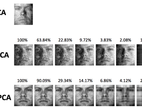
Figure 1: First Eigen Face for PCA and First Tensor Face for T-PCA and TT-PCA under different compression ratios. The number at top are the compression ratios.

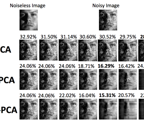
Figure 2: Face denoising under PCA, T-PCA and TT-PCA. The reconstruction errors are marked on top of each image. Different images in each row correspond to decreasing compression ratios (increasing compression, increasing $\tau$) from left to right. The compression ratios for T-PCA and TT-PCA are the same (left-right) as that in Fig. 1.

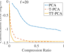
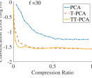
Figure 3: Clustering Error in $\log 10$ scale versus Compressed Ratio for Extended YaleFace Dataset B Dataset. 38 faces with noise are selected from the data set and the training sample size is 5, 10, 20, 30 (from left to right, top to bottom) respectively.

TABLE II: Compression ratio and classification error at the lowest classification error

Classification using TT-PCA - Next, we test the performance of the three approaches for classification. For classification, we choose $f$ training data points (at random) from each of the $38$ people, and thus the amount of training data points is $N_{\text{tr}}=38f$. The remaining data of each person is used for testing, and thus $N_{\text{te}}=38(64-f)$. We add a Gaussian noise $\mathcal{N}(0,100)$ to each pixel of the data. For training sizes $f=5,10,20,30$, Figure 3 compares the classification error of the different algorithms as a function of compression ratio for each $f$. We note that as $f$ increases, the classification performance becomes better for all algorithms. We further see that TT-PCA performs better at low compression ratios, and the classification error increases after first decreasing. This is because with higher compression ratios (low compression), the approaches will try to over-fit noise leading to lower classification accuracy.

Table II highlights the data from Figure 3 to illustrate the improved performance of TT-PCA. This table shows the compression ratio at which the best classification performance is achieved, and the classification error at this compression ratio. We note that the point at which best compression ratio is achieved is lowest for TT-PCA, and so is the best classification error thus demonstrating that TT-PCA is able to extract the data structure well at high data compressions. This indicates that human face data under different illumination conditions lies not only close to the subspace models, but are better approximated by tensor train subspace models. Further we note that TT-PCA requires far less training sample size compared to other approaches.

VI Conclusion

This paper outlines novel algorithms and methods for tensor train subspaces for data representation. A PCA like algorithm namely TT-PCA is proposed. This algorithm is validated on vision dataset and exhibit improved classification performance, better dimensionality reduction, and lower computational complexity as compared to the considered baseline approaches.

References

- [1] R. Basri and D. W. Jacobs. Lambertian reflectance and linear subspaces. IEEE transactions on pattern analysis and machine intelligence, 25(2):218–233, 2003.
- [2] M. Belkin and P. Niyogi. Laplacian eigenmaps for dimensionality reduction and data representation. Neural computation, 15(6):1373–1396, 2003.
- [3] C. M. Bishop. Pattern recognition. Machine Learning, 128, 2006.
- [4] J.-F. Cai, E. J. Candès, and Z. Shen. A singular value thresholding algorithm for matrix completion. SIAM Journal on Optimization, 20(4):1956–1982, 2010.
- [5] A. Cichocki. Era of big data processing: A new approach via tensor networks and tensor decompositions. arXiv preprint arXiv:1403.2048, 2014.
- [6] A. Cichocki, N. Lee, I. Oseledets, A. Phan, Q. Zhao, and D. Mandic. Low-rank tensor networks for dimensionality reduction and large-scale optimization problems: Perspectives and challenges part 1. arXiv preprint arXiv:1609.00893, 2016.
- [7] L. De Lathauwer, B. De Moor, and J. Vandewalle. A multilinear singular value decomposition. SIAM journal on Matrix Analysis and Applications, 21(4):1253–1278, 2000.
- [8] D. L. Donoho. De-noising by soft-thresholding. IEEE transactions on information theory, 41(3):613–627, 1995.
- [9] A. S. Georghiades, P. N. Belhumeur, and D. J. Kriegman. From few to many: Illumination cone models for face recognition under variable lighting and pose. IEEE transactions on pattern analysis and machine intelligence, 23(6):643–660, 2001.
- [10] S. Holtz, T. Rohwedder, and R. Schneider. On manifolds of tensors of fixed tt-rank. Numerische Mathematik, 120(4):701–731, 2012.
- [11] I. Jolliffe. Principal component analysis. Wiley Online Library, 2002.
- [12] K.-C. Lee, J. Ho, and D. J. Kriegman. Acquiring linear subspaces for face recognition under variable lighting. IEEE Transactions on pattern analysis and machine intelligence, 27(5):684–698, 2005.
- [13] H. Lu, K. N. Plataniotis, and A. N. Venetsanopoulos. Multilinear principal component analysis of tensor objects for recognition. In 18th International Conference on Pattern Recognition (ICPR’06), volume 2, pages 776–779. IEEE, 2006.
- [14] H. Lu, K. N. Plataniotis, and A. N. Venetsanopoulos. Uncorrelated multilinear principal component analysis for unsupervised multilinear subspace learning. IEEE Transactions on Neural Networks, 20(11):1820–1836, 2009.
- [15] H. Lu, K. N. Plataniotis, and A. N. Venetsanopoulos. A survey of multilinear subspace learning for tensor data. Pattern Recognition, 44(7):1540–1551, 2011.
- [16] I. V. Oseledets. Tensor-train decomposition. SIAM Journal on Scientific Computing, 33(5):2295–2317, 2011.
- [17] D. Perez-Garcia, F. Verstraete, M. M. Wolf, and J. I. Cirac. Matrix product state representations. arXiv preprint quant-ph/0608197, 2006.
- [18] M. A. O. Vasilescu and D. Terzopoulos. Multilinear subspace analysis of image ensembles. In Computer Vision and Pattern Recognition, 2003. Proceedings. 2003 IEEE Computer Society Conference on, volume 2, pages II–93. IEEE, 2003.
- [19] R. Vidal, Y. Ma, and S. Sastry. Generalized principal component analysis (gpca). IEEE Transactions on Pattern Analysis and Machine Intelligence, 27(12):1945–1959, 2005.
- [20] W. Wang, V. Aggarwal, and S. Aeron. Tensor completion by alternating minimization under the tensor train (tt) model. arXiv preprint arXiv:1609.05587, 2016.
- [21] W. Wang, V. Aggarwal, and S. Aeron. Tensor train neighborhood preserving embedding. arXiv preprint arXiv:1712.00828, 2017.
- [22] S. Yan, D. Xu, Q. Yang, L. Zhang, X. Tang, and H.-J. Zhang. Multilinear discriminant analysis for face recognition. IEEE Transactions on Image Processing, 16(1):212–220, 2007.
- [23] R. Zeng, J. Wu, Z. Shao, L. Senhadji, and H. Shu. Multilinear principal component analysis network for tensor object classification. arXiv preprint arXiv:1411.1171, 2014.