On Computing Jacobi’s Elliptic Function sn

Abstract

The paper presents a method to compute the Jacobi’s elliptic function sn on the period parallelogram. For fixed $m$ it requires first to compute the complete elliptic integrals $K=K(m)$ and $K^{\prime}=K(1-m).$ The Newton method is used to compute $\mathrm{sn}(z,m),$ when $z\in[0,K]\cup[0,iK^{\prime}).$ The computation in any other point does not require the usage of any numerical procedure, it is done only with the help of the properties of $\mathrm{sn}.$

2010 Mathematics Subject Classification: 65D20, 33F05.

Key words: elliptic functions, elliptic integrals, arithmetic-geometric mean,

1 Introduction

The paper presents a method to compute the Jacobi’s elliptic function sn on the period parallelogram. For fixed $m\in(0,1)$ it requires first to compute the complete elliptic integrals $K=K(m)$ and $K^{\prime}=K(1-m).$ The function to compute the first complete elliptic integral uses the arithmetic-geometric mean, as a consequence of Gauss’s theorem.

The Newton method to solve a nonlinear algebraic equation is used to compute $\mathrm{sn}(z,m),$ when $z\in[0,K]\cup[0,iK^{\prime}).$ The computation in any other point does not require the usage of any numerical procedure, it is done only with the help of the properties of $\mathrm{sn}$ and its values on some points from $[0,K]\cup i[0,K^{\prime}).$

The validity of the method is exemplified with the help of a Scilab application. The obtained results are very good approximations of the values given by the corresponding functions from Scilab and Mathematica.

The computation of the elliptic integrals and of the elliptic functions were studied in many papers, e.g. [2], [3], [5], as well as the included bibliography.

2 Incomplete elliptic integral of first kind

The following incomplete and complete elliptic integrals of first kind are defined respectively by, [9],

$$F(\phi,m)=\int_{0}^{\sin{\phi}}\frac{\mathrm{d}t}{\sqrt{(1-t^{2})(1-mt^{2})}}=\int_{0}^{\phi}\frac{\mathrm{d}\theta}{\sqrt{1-m\sin^{2}\theta}}$$

and

$$K(m)=\int_{0}^{1}\frac{\mathrm{d}t}{\sqrt{(1-t^{2})(1-mt^{2})}}=F(\frac{\pi}{2},m).$$

In order to compute $F(\phi,m)$ we recall a result established by Carl Friedrich GAUSS (1777-1855) in 1799, [7], [1]:

Theorem 2.1

If $a$ and $b$ are positive reals and $M(a,b)$ is their the arithmetic-geometric mean then

$$\frac{1}{M(a,b)}=\frac{2}{\pi}\int_{0}^{\frac{\pi}{2}}\frac{\mathrm{d}x}{\sqrt{a^{2}\cos^{2}{x}+b^{2}\sin^{2}{x}}}.$$ (1)

For $a>b>0$ and $0\leq\phi\leq\frac{\pi}{2}$ we shall take care of the integral

$$I(a,b,\phi)=\int_{0}^{\phi}\frac{\mathrm{d}x}{\sqrt{a^{2}\cos^{2}{x}+b^{2}\sin^{2}{x}}}=\frac{1}{a}\int_{0}^{\phi}\frac{\mathrm{d}x}{\sqrt{1-\left(1-\frac{b^{2}}{a^{2}}\right)\sin^{2}{x}}}=$$ (2)

$$=\frac{1}{a}F\left(\phi,1-\frac{b^{2}}{a^{2}}\right)$$

and

$$I(a,b,\frac{\pi}{2})=\frac{1}{a}K\left(1-\frac{b^{2}}{a^{2}}\right).$$

Thus, the equality (2) may be rewritten as $\frac{1}{M(a,b)}=\frac{2}{a\pi}K\left(1-\frac{b^{2}}{a^{2}}\right)$ or

$$K\left(1-\frac{b^{2}}{a^{2}}\right)=\frac{\pi}{2}\frac{1}{\frac{1}{a}M(a,b)}=\frac{\pi}{2}\frac{1}{M(1,\frac{b}{a})}.$$

As in [7], for $I(a,b,\phi)$ the changing of variables

$$\sin{x}=\frac{2a\sin{\varphi}}{a+b+(a-b)\sin^{2}{\varphi}}$$

leads to the sequence

$$I(a,b,\phi)\stackrel{{\scriptstyle def}}{{=}}I_{0}(a_{0},b_{0},\phi_{0})=I_{1}(a_{1},b_{1},\phi_{1})=I_{2}(a_{2},b_{2},\phi_{2})=\ldots$$ (3)

where

$$I_{k}(a_{k},b_{k},\phi_{k})=\int_{0}^{\phi_{k}}\frac{\mathrm{d}\varphi}{\sqrt{a_{k}^{2}\cos^{2}{\varphi}+b_{k}^{2}\sin^{2}{\varphi}}}$$

and the upper integration limits are generated by the sequence

$$\sin{\phi_{k-1}}=\frac{2a_{k-1}\sin{\phi_{k}}}{a_{k-1}+b_{k-1}+(a_{k-1}-b_{k-1})\sin^{2}{\phi_{k}}}.$$

The sequence $(\sin{\phi_{k}})_{k\in\mathbb{N}}$ is decreasing and consequently the sequence $(\phi_{k})_{k\in\mathbb{N}}$ is convergent. It results that

$$\sin{\phi_{k}} = a_{k-1}-\frac{\sqrt{a_{k-1}^{2}\cos^{2}{\phi_{k-1}}+b_{k-1}^{2}\sin^{2}{\phi_{k-1}}}}{(a_{k-1}-b_{k-1})\sin{\phi_{k-1}}}=y_{k}$$ (4)

$$\phi_{k} = \arcsin{y_{k}}.$$

From (3) it results

$$I(a,b,\phi)=\lim_{k\rightarrow\infty}I_{k}(a_{k},b_{k},\phi_{k})=\frac{\phi_{\infty}}{M(a,b)},$$

with $\phi_{\infty}=\lim_{k\rightarrow\infty}\phi_{k}.$ Using (2) we get

$$I(a,b,\phi)=\frac{1}{a}F\left(\phi,1-\frac{b^{2}}{a^{2}}\right)=\frac{\phi_{\infty}}{M(a,b)}$$

and consequently

$$F\left(\phi,1-\frac{b^{2}}{a^{2}}\right)=\frac{a\phi_{\infty}}{M(a,b)}=\frac{\phi_{\infty}}{\frac{1}{a}M(a,b)}=\frac{\phi_{\infty}}{M(1,\frac{b}{a})}.$$

Denoting $m=1-\frac{b^{2}}{a^{2}},(a>b>0\ \Leftrightarrow\ 0<m<1),$ the above equation becomes

$$F(\phi,m)=\frac{\phi_{\infty}}{M(1,\sqrt{1-m})}.$$ (5)

Therefore the computation of $F(\phi,m)$ returns to generate iteratively the sequences $(a_{k})_{k},\ (b_{k})_{k},\ (\phi_{k})_{k}$ until a stopping condition is fulfilled. The initial values are $a_{0}=1,\ b_{0}=\sqrt{1-m}$ and $\phi_{0}=\phi.$ For $a_{0}=1,$ instead of the sequences $(a_{k})_{k},\ (b_{k})_{k}$ we may compute the sequences, [8],

$$\begin{array}[]{l}s_{0}=b_{0}\\ s_{k+1}=\frac{2\sqrt{s_{k}}}{1+s_{k}}\end{array}\qquad\begin{array}[]{l}p_{0}=\frac{1}{2}(1+s_{0})\\ p_{k+1}=\frac{1}{2}(1+s_{k})p_{k}\end{array}.$$

Then $\lim_{k\rightarrow\infty}p_{k}=M(1,b_{0}).$

If $\phi=\frac{\pi}{2}$ then $\phi_{\infty}=\frac{\pi}{2}$ and we retrieve

$$K(m)=\frac{\pi}{2M(1,\sqrt{1-m})}.$$ (6)

From a practical point of view and as a drawback the method is not applicable when $\phi$ is small, e.g. $0<\phi<10^{-5}.$ The cause is the presence of the factor $\sin{\phi_{k-1}}$ in the denominator in (4). In this case, from the Maclaurin series expansion of $F(\phi,m)$ we get $F(\phi,m)\approx\phi-\frac{m}{6}\phi^{3}.$

3 The Jacobi elliptic function sn

The Jacobi elliptic function $\mathrm{sn}(z,m)$ may be defined by the equation, [1],

$$z=\int_{0}^{\mathrm{sn}(z,m)}\frac{\mathrm{d}t}{\sqrt{(1-t^{2})(1-mt^{2})}}.$$ (7)

Throughout this paper the variable $m$ is fixed and we use the shorter notation $\mathrm{sn}(z),$ omitting $m.$

We shall use the following Jacobi elliptic functions, too

$$\mathrm{cn}^{2}(z)=1-\mathrm{sn}^{2}(z),\qquad\mathrm{dn}^{2}(z,m)=1-m\ \mathrm{sn}^{2}(z).$$

Again we shall use the shorter notation $\mathrm{dn}(z).$

If

$$K=K(m)\qquad\mbox{and}\qquad K^{\prime}=K(1-m)$$

then the parallelogram period is the rectangle $D=[0,4K)+i[0,2K^{\prime})$ and the points $K^{\prime}i$ and $2K+iK^{\prime}$ are poles of first order, [8].

The following properties of the function $\mathrm{sn}$ will be used, [8], [6]:

• $$\mathrm{sn}(-z)=-\mathrm{sn}(z)$$ (8)

• $$\mathrm{sn}(x+y) = \frac{\mathrm{sn}(x)\mathrm{cn}(y)\mathrm{dn}(y)+\mathrm{sn}(y)\mathrm{cn}(x)\mathrm{dn}(x)}{1-m\ \mathrm{sn}^{2}(x)\mathrm{sn}^{2}(y)}$$ (9)

  $$\mathrm{cn}(x+y) = \frac{\mathrm{cn}(x)\mathrm{cn}(y)-\mathrm{sn}(x)\mathrm{sn}(y)\mathrm{dn}(x)\mathrm{dn}(y)}{1-m\ \mathrm{sn}^{2}(x)\mathrm{sn}^{2}(y)}$$ (10)

  $$\mathrm{dn}(x+y) = \frac{\mathrm{dn}(x)\mathrm{dn}(y)-m\ \mathrm{sn}(x)\mathrm{sn}(y)\mathrm{cn}(x)\mathrm{cn}(y)}{1-m\ \mathrm{sn}^{2}(x)\mathrm{sn}^{2}(y)}$$ (11)

• Because $\mathrm{sn}(K)=1,\ \mathrm{cn}(K)=0,\ \mathrm{dn}(K)=\sqrt{1-m}$ from the above equalities it results

  $$\mathrm{sn}(K\pm z) = \frac{\mathrm{cn}(z)}{\mathrm{dn}(z)}$$ (12)

  $$\mathrm{cn}(K+z) = -\sqrt{1-m}\frac{\mathrm{sn}(z)}{\mathrm{dn}(z)}$$ (13)

  $$\mathrm{dn}(K+z) = \frac{\sqrt{1-m}}{\mathrm{dn}(z)}$$ (14)

• Knowing that $\mathrm{sn}(2K)=0,\mathrm{cn}(2K)=-1,\mathrm{dn}(2K)=1$, from (9) it results

  $$\mathrm{sn}(2K\pm z)=\mp\mathrm{sn}(z)$$ (15)

• Knowing that $\mathrm{sn}(K+iK^{\prime})=\frac{1}{\sqrt{m}},\mathrm{dn}(K+iK^{\prime})=0$ from (9) it results

  $$\mathrm{sn}(z+K+iK^{\prime})=\frac{1}{\sqrt{m}}\ \frac{\mathrm{dn}(z)}{\mathrm{cn}(z)}.$$ (16)

The computation of $\mathrm{sn}(z)$ depends on the position of $z$ in $D$ and we suppose that we know $K$ and $K^{\prime}.$

• If $z\in[0,K]$ or $z\in i[0,K^{\prime})$ then $\mathrm{sn}(z)$ will be the solution $u$ of the equation

  $$\Phi(u)=\int_{0}^{u}\frac{\mathrm{d}t}{\sqrt{(1-t^{2})(1-mt^{2})}}-z=0.$$ (17)

• Otherwise and excepting the poles the value of $\mathrm{cn}(z)$ will be computed using the properties of the function $\mathrm{sn}$ and its values on some points from $[0,K]\cup i[0,K^{\prime}),$ without any other additional numerical procedure.

Computing $\mathrm{sn}(z)$ in the segment $[0,4K)$

The following cases arise:

1. $z\in[0,K].$ Equation (17) may be solved using the Newton method with the iterations

   $$u_{k+1}=u_{k}-\frac{\Phi(u_{k})}{\Phi^{\prime}(u_{k})}=u_{k}-\left(F(\arcsin{u_{k}},m)-z\right)\sqrt{(1-u_{k}^{2})(1-mu_{k}^{2})}$$

   The linear interpolation between $\mathrm{sn}(z,0)$ and $\mathrm{sn}(z,1)$ gives the initial approximation $u_{0}=(1-m)\sin{z}+m\tanh{z}.$

   If $z$ is small enough the method is rapidly converging and for $z$ near $K$ we set $z^{\prime}=K-z$ and after computing $\mathrm{sn}(z^{\prime})=w^{\prime}$ as was described above, using (12) we have

   $$\mathrm{sn}(z)=\mathrm{sn}(K-z^{\prime})=\frac{\mathrm{cn}(z^{\prime})}{\mathrm{dn}(z^{\prime})}=\sqrt{\frac{1-w^{\prime 2}}{1-m\ w^{\prime 2}}}.$$

2. $z\in(K,4K).$ Let be

   $$z^{\prime}=\left\{\begin{array}[]{lcl}2K-z&\mbox{if}&z\in(K,2K]\\ z-2K&\mbox{if}&z\in(2K,3K]\\ 4K-z&\mbox{if}&z\in(3K,4K)\end{array}\right..$$

   After computing $\mathrm{sn}(z^{\prime})=w^{\prime},\ z^{\prime}\in[0,K],$ we have

   $$\mathrm{sn}(z)=\left\{\begin{array}[]{lcl}w^{\prime}&\mbox{if}&z\in(K,2K]\\ -w^{\prime}&\mbox{if}&z\in(2K,4K)\end{array}\right..$$

   Indeed, if $z\in(K,2K]$ then

   $$\mathrm{sn}(z)=\mathrm{sn}(2K-z^{\prime})=\mathrm{sn}(z^{\prime})=w^{\prime};$$

   if $z\in(2K,3K]$ then

   $$\mathrm{sn}(z)=\mathrm{sn}(2K+z^{\prime})=-\mathrm{sn}(z^{\prime})=-w^{\prime}$$

   and if $z\in(3K,4K)$ then

   $$\mathrm{sn}(z)=\mathrm{sn}(4K-z^{\prime})=\mathrm{sn}(-z^{\prime})=-\mathrm{sn}(z^{\prime})=-w^{\prime}.$$

Computing $\mathrm{sn}(z)$ for $z\in i(0,2K^{\prime})\setminus\{iK^{\prime}\}.$

The following cases arise:

1. $z\in i[0,K^{\prime}).$ Writing $z=iy,\ y\in[0,K^{\prime}),$ we are looking for the solution of the equation (17) in the form $u=iv,v\in\mathbb{R}.$ After the change of variable $t=is$ there is obtained the equation

   $$\Psi(v)=\int_{0}^{v}\frac{\mathrm{d}s}{\sqrt{(1+s^{2})(1+m\ s^{2})}}-y=0.$$ (18)

   According to the Newton method, the iterations are

   $$v_{k+1}=v_{k}-\frac{\Psi(v_{k})}{\Psi^{\prime}(v_{k})}=$$

   $$=v_{k}-\left(\int_{0}^{v_{k}}\frac{\mathrm{d}s}{\sqrt{(1+s^{2})(1+m\ s^{2})}}-y\right)\sqrt{(1+v_{k}^{2})(1+m\ v_{k}^{2})}$$

   starting with $v_{0}=y.$ The above integral is computed using a quatrature procedure.

2. $z\in i(K^{\prime},2K^{\prime}].$ Let be $z^{\prime}=z-iK^{\prime}=iy^{\prime}$ with $y^{\prime}\in(0,K^{\prime}).$ From (16) we have

   $$\mathrm{sn}(z)=\mathrm{sn}(iK^{\prime}+iy^{\prime})=\frac{1}{\sqrt{m}}\ \frac{\mathrm{dn}(iy^{\prime}-K)}{\mathrm{cn}(iy^{\prime}-K)}.$$

   After using (13) and (14) it results

   $$\mathrm{sn}(z)=\frac{1}{\sqrt{m}\ \mathrm{sn}(z^{\prime})}.$$

Computing $\mathrm{sn}(z)$ in the rectangle period

We describe here how to compute $\mathrm{sn}(z)$ when $z$ belongs to the rectangle period excepting the poles and the lower and the left sides.

Let $z=x+iy$ such that $x\in(0,4K)$ and $y\in(0,2K^{\prime}).$

The following cases arise:

1. $y\not=K^{\prime}.$ Using (9) we have

   $$\mathrm{sn}(z)=\mathrm{sn}(x+iy)=\frac{\mathrm{sn}(x)\mathrm{cn}(iy)\mathrm{dn}(iy)+\mathrm{sn}(iy)\mathrm{cn}(x)\mathrm{dn}(x)}{1-m\ \mathrm{sn}^{2}(x)\mathrm{sn}^{2}(iy)}.$$

   $\mathrm{sn}(x),\mathrm{sn}(iy)$ are computed as was presented above and then compute $\mathrm{cn}(x),\mathrm{cn}(iy),\mathrm{dn}(x),\mathrm{dn}(iy).$ It must be taken into account that if $x\in(K,3K)$ then $\mathrm{cn}(x)=-\sqrt{1-\mathrm{sn}^{2}(x)}.$

2. $y=K^{\prime}.$ We deduce through (14)

   $$\mathrm{sn}(z)=\mathrm{sn}(K+iK^{\prime}+x-K)=\frac{1}{\sqrt{m}}\ \frac{\mathrm{dn}(x-K)}{\mathrm{cn}(x-K)}.$$

   As above, applying (13) and (14) we obtain

   $$\mathrm{sn}(z)=\frac{1}{\sqrt{m}\ \mathrm{sn}(x)}.$$

On poles, $z\in\{iK^{\prime},2K+iK^{\prime}\},$ we set $\mathrm{sn}(z)=\infty.$

In his way we have computed the value of $\mathrm{sn}(z)$ for any $z\in D.$

4 Numerical results

Numeric computing softwares contains functions to compute elliptical integrals and elliptical functions. We recall some methods in Mathematica and Scilab in Table 1.

Meaning	Function signature
Mathematica
$F(\phi,m)$	EllipticF[$\phi,m$]
$K(m)$	EllipticK[$m$]
$\mathrm{sn}(z,m)$	JacobiSN[$z,m$]
$\mathrm{cn}(z,m)$	JacobiCN[$z,m$]
$\mathrm{dn}(z,m)$	JacobiDN[$z,m$]
Scilab
$F(\phi,m)$	delip($\phi,\sqrt{m}$)
$\mathrm{sn}(z,m)$	%$\mathrm{sn}(z,m)$

Table 1: Elliptical function in Mathematica and Scilab.

We developed a Scilab program based on the method presented in this paper. The values $K$ and $K^{\prime}$ were computed using (6). Because the numbers have a floating point representation two numbers are considered to be equal if their distance is less than a tolerance.

Some results are given in Table 2. The function JacobiSN from Mathematica gives similar values (excepting the poles).

$z$	$\mathrm{sn}(z)$ computed	%$\mathrm{sn}(z,m)$	Error
			$|\mathrm{sn}(z)-\%\mathrm{sn}(z,m)|$
$m=0.81$
K=2.2805491	delip$(1,0.9)=2.2805491$		$4.441D-16$
K’=1.6546167	delip$(1,\sqrt{0.19})=1.6546167$		$2.220D-16$
$0.5K$	0.8345252	0.8345252	1.024D-09
$1.4K$	0.9038225	0.9038225	6.602D-10
$2.7K$	-0.9501563	-0.9501563	7.363D-10
$3.3K$	-0.9501563	-0.9501563	7.363D-10
$i0.6K^{\prime}$	1.4511449i	1.4511449i	1.554D-15
$i1.3K^{\prime}$	-2.0696167i	-2.0696167i	1.332D-15
$0.8K+i0.3K^{\prime}$	1.0085488 + 0.0420829i	1.0085488 + 0.0420829i	5.812D-10
$0.5K+i1.7K^{\prime}$	0.9048397 - 0.1679796i	0.9048397 - 0.1679796i	1.129D-09
$1.3K+i1.7K^{\prime}$	0.9892195 + 0.071665i	0.9892195 + 0.071665i	2.701D-10
$2.5K+i0.4K^{\prime}$	-0.9592212 - 0.2093038i	-0.9592212 - 0.2093038i	8.724D-10
$3.6K+i0.4K;$	-0.8951883 + 0.3091877i	-0.8951883 + 0.3091877i	1.656D-09
$3.6K+i1.7K^{\prime}$	-0.8233279 - 0.2419397i	-0.8233279 - 0.2419397i	1.519D-09
$0.5K+iK^{\prime}$	1.3314291	1.3314291	1.634D-09
$2.5K+iK^{\prime}$	-1.3314291	-1.3314291	1.183D-09
$K+iK^{\prime}$	1.1111111	1.1111111	2.220D-16
$K$	1.	1.	2.220D-16
$iK^{\prime}$	Nan + Infi	1.633D+16i	Nan
$2K+iK^{\prime}$	Nan + Infi	-4.211D+15 + 1.170D+15i	Nan

Table 2: Results obtained using the presented method.

The 3D image of the modules of the function $\mathrm{sn}(z,0.81)$ computed on $D$ is given in Figure 1.

Finally we show the visualization of the complex function, using the method presented in [4]. In a point the value of the function is represented by a color obtained projecting that value into the colors cube. The procedure is based on the stereographic projection.

The Figure 2 is given for calibration, representing the visualization of the identity function.

The Figure 3 contains the visualization of $\mathrm{sn}(z,0.81),\ z\in D.$ The zeros are colored in black while the poles are colored in white.

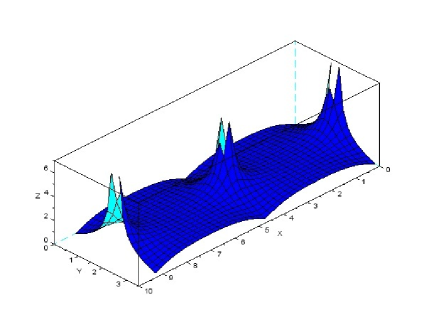
Figure 1: For $m=0.81$ the 3D image of the modules of $\mathrm{sn}$.

Figure 2: Function $w\mapsto w,w\in[-5,5]+i[-5,5]$

Figure 3: Function $w=\mathrm{sn}(z,0.81),z\in D$.

References

• [1] BORWEIN J.M., BORWEIN P.B., Pi and the AGM. John Wiley & Sons, New York, 1986.
• [2] FUKUSHIMA T., Numerical computation of inverse complete elliptic integrals of first and second kinds. J. Computation and Applied Mathematics, 249 (2013), 37-50.
• [3] FUKUSHIMA T. Fast computation of complete elliptic integrals and Jacobian elliptic functions. Celest Mech Dyn Astr (2009) 105: 305. https://doi.org/10.1007/s10569-009-9228-z.
• [4] RICHARDSON J.L., Visualizing Complex Functions. 2003, http://web.archive.org/web/20030802162645/http://physics.hallym.ac.kr/education/.
• [5] R$\ddot{\mathrm{O}}$SCH N., The derivation of algorithms to compute elliptic integrals of the first and second kind by Landen transformation. Boletin de Ciências Geodésicas (Online), 17 (2011), no.1, http://dx.doi.org/10.1590/S1982-21702011000100001.
• [6] SNAPE J., Applications of Elliptic Functions in Classical and Algebraic Geometry. Collingwood College, University of Durham, Master thesis, 2000. https://wwwx.cs.unc.edu/~snape/publications/mmath/.
• [7] TKACHEV V.G., Elliptic functions: Introduction course. http://users.mai.liu.se/vlatk48/teaching/lect2-agm.pdf.
• [8] WHITTAKER E.T., WATSON G.,N., A Course of Modern Analysis. Cambridge University Press, 1920.
• [9] * * *, NIST Digital Library of Mathematical Functions. http://dlmf.nist.gov/, Release 1.0.17 of 2017-12-22. F. W. J. Olver, A. B. Olde Daalhuis, D. W. Lozier, B. I. Schneider, R. F. Boisvert, C. W. Clark, B. R. Miller, and B. V. Saunders, eds.