Stellar obliquities and magnetic activities of Planet-Hosting Stars and Eclipsing Binaries based on Transit Chord Correlation

Abstract

The light curve of an eclipsing system shows anomalies whenever the eclipsing body passes in front of active regions on the eclipsed star. In some cases, the pattern of anomalies can be used to determine the obliquity $\Psi$ of the eclipsed star. Here we present a method for detecting and analyzing these patterns, based on a statistical test for correlations between the anomalies observed in a sequence of eclipses. Compared to previous methods, ours makes fewer assumptions and is easier to automate. We apply it to a sample of 64 stars with transiting planets and 24 eclipsing binaries for which precise space-based data are available, and for which there was either some indication of flux anomalies or a previously reported obliquity measurement. We were able to determine obliquities for ten stars with hot Jupiters. In particular we found $\Psi\lesssim$10^∘ for Kepler-45, which is only the second M dwarf with a measured obliquity. The other 8 cases are G and K stars with low obliquities. Among the eclipsing binaries, we were able to determine obliquities in 8 cases, all of which are consistent with zero. Our results also reveal some common patterns of stellar activity for magnetically active G and K stars, including persistently active longitudes.

1. Introduction

The Solar System is nearly coplanar, with the Sun’s equator and the planetary orbits aligned to within a few degrees. This makes sense because the Sun and the planets likely formed from a flattened disk of material with a well-defined sense of rotation. However, the discovery of planets with orbits nearly perpendicular to the star’s equator (e.g., HAT-P-11b, Winn et al., 2010b), or nearly retrograde (e.g., WASP-17b, Triaud et al., 2010) show that planet formation and evolution can be more complicated than in this simple picture. There is hope that the distribution of obliquities, and its dependence on stellar and planetary properties, will help to elucidate the formation history and orbital evolution of planets (as recently reviewed by Winn & Fabrycky, 2015; Triaud, 2017). Many methods are available for measuring stellar obliquities: the Rossiter-McLaughlin effect (Queloz et al., 2000); the $v\rm{sin}i_{\star}$ method (Schlaufman, 2010; Winn et al., 2017); the photometric variability method (Mazeh et al., 2015b); the gravity-darkening method (Barnes, 2009; Masuda, 2015); the asteroseismic method (Chaplin et al., 2013; Huber et al., 2013; Van Eylen et al., 2014); and the method based on spot-crossing anomalies (Sanchis-Ojeda et al., 2011; Désert et al., 2011; Mazeh et al., 2015a; Holczer et al., 2015), the subject of this paper.

When a transiting planet is blocking a dark starspot, the loss of light is smaller than when it is blocking an unspotted portion of the photosphere. This produces a positive glitch in the light curve. Similarly, transits over bright regions (plages and faculae) produce negative glitches. In some cases the stellar obliquity can be deduced from the pattern of recurrence of spot-crossing anomalies in a sequence of transits. As a simple example, consider a low-obliquity star with long-lived starspots and a rotation period $P_{\rm rot}$ much longer than the planet’s orbital period $P_{\rm orb}$. In such a case, the anomalies that are seen during one transit will recur in the next transit, but shifted forward in time because the active regions have advanced across the the visible hemisphere of the star due to stellar rotation. Conversely, if the stellar obliquity is high, the rotation of the star carries the active regions outside of the “transit chord”, the narrow strip on the stellar disk that is traversed by the transiting planet. In this case, the anomalies produced by a given spot will not recur in subsequent transits.

Unlike some of the other methods for measuring obliquities, the spot-crossing method does not require high-resolution spectroscopy, and can therefore be applied to relatively faint stars. However, the spot-crossing method does require a large number of consecutive light curves with a high signal-to-noise ratio (SNR) to allow spot-crossing events and their recurrence to be detected. As a result, it has only been applied to about a dozen systems. Most of these were discovered by the space missions CoRoT and Kepler. The method of analysis has generally relied on the identification of discrete anomalies, often through visual inspection, a laborious and somewhat subjective procedure. Most of the modeling has been performed with idealized assumptions such as circular spots of uniform intensity.

The motivation for our work was to develop a more objective method that does not rely on explicit spot modeling, and can be more easily applied to a large sample of systems. Instead of assuming that the active regions are discrete dark and bright spots, we treat the transit light curve as a measure of the intensity distribution of the stellar photosphere along the transit chord. We do not model the intensity distribution with discrete spots, although we still must hope that the active regions persist and are nearly stationary in the rotating frame of the star for at least a few orbital periods. Given the values of $P_{\rm rot}$ and $P_{\rm orb}$, we can calculate the angle by which the active regions should advance in between transits if the obliquity is low. Then we can seek evidence for correlations — with the appropriate lag — between the anomalies observed in a series of transits. A significant correlation implies a low obliquity. We can search for evidence of retrograde rotation in a similar way.

For convenience we call this the Transit Chord Correlation (TCC) method, although we do not claim it is a completely new concept. It is closely related to eclipse mapping (Horne, 1985), which has long been used to probe the brightness distribution of stars and accretion disks. Eclipse mapping has also been applied to a couple of stars with transiting planets (Huber et al., 2010; Scandariato et al., 2017). The main difference is that the previous investigators assumed zero obliquity and sought to determine the brightness distribution across the transit chord, while we use the method to try and determine the obliquity.

Similar in spirit to our method is the one described by Mazeh et al. (2015a) and Holczer et al. (2015). They were able to distinguish prograde and retrograde motion in a few Kepler systems by searching for a significant correlation between the observed transit timing variations (TTV) and the time derivative of the stellar flux immediately before and after transits. Stars with prograde rotation should show a correlation if a single active region is responsible for both the apparent TTV and the out-of-transit variation, while retrograde stars should show an anti-correlation. Two advantages of this method are its simplicity and the freedom from the requirement that the active regions have a lifetime of a few orbital periods. One problem is that the out-of-transit variations are the net effect of all the active regions on the star, and are not necessarily dominated by the region that is responsible for the transit anomalies. Our TCC method does not rely on the out-of-transit variations, and is also able to provide higher precision in the obliquity determination.

In this paper, we explain the TCC method, validate it through application to systems for which the stellar obliquity has been measured by independent methods, and apply it to all the transiting planets for which the method is currently feasible. We also apply the TCC method to a sample of eclipsing binaries drawn from the Kepler survey. Section 2 describes the TCC method in greater detail. Section 3 describes the target selection and light curve preparation and analysis. Section 4 presents the results for the obliquities, as well as some interesting features we noticed in the pattern and time evolution of active regions. Section 5 discusses these results in the context of what was previously known about both stellar obliquities and stellar activity.

2. Method

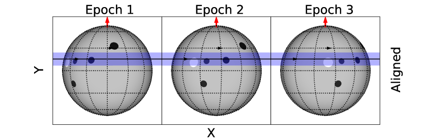
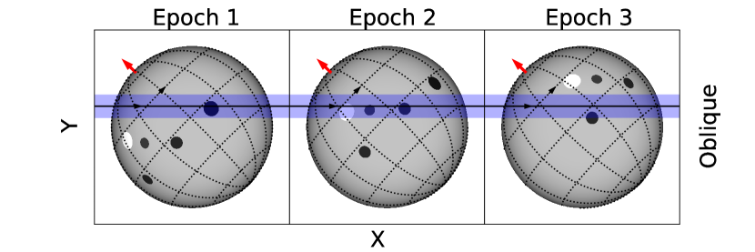
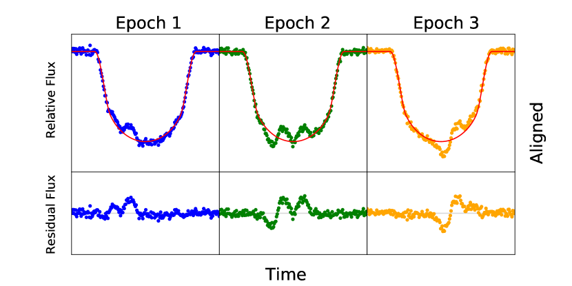
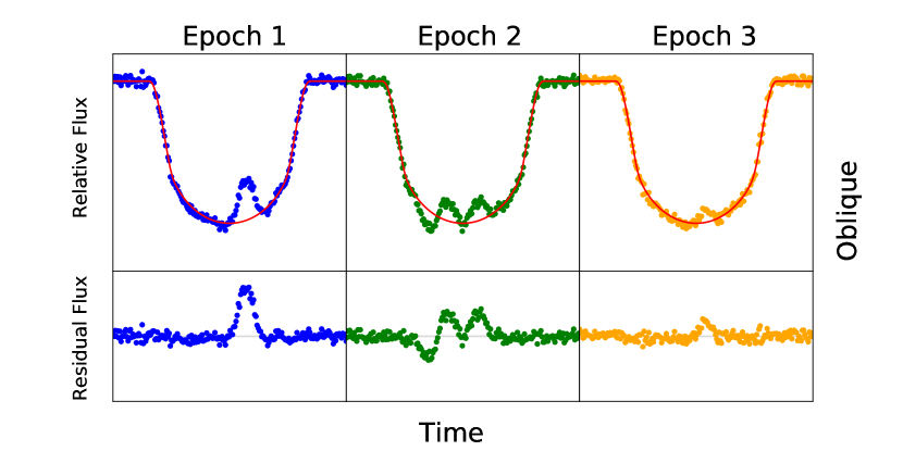
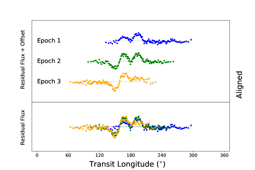
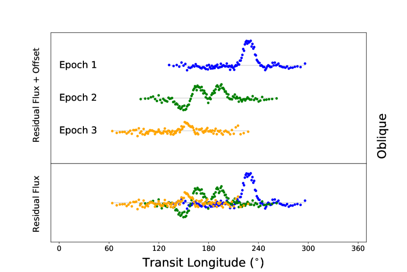
Figure 1.— Top: Transits of a planet across a star with active regions. The red arrows and dotted lines convey the orientation of the rotating host star. The solid line is the trajectory of the transiting planet and the blue bar is the transit chord. The black and white circles are active regions (spots and faculae) on the host star. Three consecutive transits are shown, for each of two different geometries: “Aligned” with stellar obliquity $\Psi\approx 0^{\circ}$, and “Oblique” with $\Psi\approx 45^{\circ}$. The two cases are initialized such that the light curves are identical in Epoch 2.
Middle: Corresponding light curves. A glitch occurs when the planet transits across an active region. The red solid curves are the best-fitting transit models, which do not account for the active regions. When $\Psi\approx 0^{\circ}$, the anomalies advance in time from one transit to the next, due to stellar rotation.
Bottom: Residual flux as a function of transit longitude. Knowing the stellar rotation period, we transform the time stamps of the data into the transit longitude (see Equation 1). In the Aligned case, the planet repeatedly eclipses the same set of active regions, leading to recurring glitches in the residual flux at the same transit longitudes. In the Oblique case, the active regions rotate outside of the transit chord. No recurring patterns are observed. The Transit Chord Correlation method looks for statistically significant correlations in the residuals as a function of transit longitude.

2.1. Conceptual illustration

Figure 1 illustrates the concept of the TCC method. This figure shows the face of a star and the corresponding light curves of three consecutive transits. On the left are the light curves for a well-aligned star ($\Psi\approx 0^{\circ}$) with a random pattern of active regions that slowly rotates across the visible hemisphere. The anomalies are seen to move progressively to the right along the time axis. We isolate the anomalies by subtracting the best-fitting transit model. Then we transform the time coordinate into the longitude $\Phi$ of the star that is being crossed by the planet, using the equation

$$\Phi(t)=\sin^{-1}\left[\frac{x(t)}{\sqrt{1-y(t)^{2}}}\right]-\frac{2\pi(t-t_{\rm ref})}{P_{\text{rot}}}$$ (1)

where $x(t)$ and $y(t)$ are the sky-plane coordinates of the planet in the system defined by Winn (2010), in which the origin is at the center of the stellar disk and the $x$ direction is aligned with the planet’s trajectory. The reference time $t_{\rm ref}$ is arbitrary; we adopt the usual Kepler convention of BJD 2454833. Note that $\Phi$ is the longitude of the star in its own rotating frame. Thus, active regions maintain a constant value of $\Phi$ even as they rotate across the star’s visible hemisphere, as long as they do not evolve or migrate significantly on the timescale of the orbital period of the planet (typically 1–10 days, for the planets considered in this work). We also note that this transformation assumes that $P_{\rm rot}$ is a constant and thereby neglects the effects of latitudinal differential rotation. When the star has a low obliquity, $P_{\rm rot}$ should be understood as the rotation period at the latitude of the transit chord.

Now that we have calculated the stellar longitude that is being blocked by the planet as a function of time, we can plot the light-curve residuals as a function of stellar longitude. This is shown in the bottom panels of Figure 1. The three patterns of residuals are seen to be very similar, as expected, since we have assumed that the active regions are stationary in the star’s reference frame. The slight change of the observed pattern between transits are caused by geometric foreshortening and limb darkening of the active regions. In this well-aligned case, we would observe strong correlations between the residuals of successive transits.

The right side of Figure 1 shows similar illustrations for a star that has an obliquity $\Psi$ of 45^∘. In this case, the active regions rotate across the transit chord, rather than along the chord. When a naive observer transforms time into stellar longitude under the assumption $\Psi\approx 0^{\circ}$, the residuals show no correlation. This is because the anomalies that are seen in successive transits are produced by different active regions. In this case $\Phi$, as calculated by Equation 1, is not really the stellar longitude. To be more general we will refer to $\Phi$ as the transit longitude rather than the stellar longitude; it corresponds to the stellar longitude only when the star has a low obliquity.

The TCC (defined below) is a statistic that quantifies the degree of correlation between the residuals of successive transits as a function of transit longitude. If the obliquity is low and the SNR is high enough, the TCC should be high when the correct stellar rotation period $P_{\rm rot}$ is used to calculated $\Phi$ in Equation 1. The high TCC indicates there is a pattern of active regions beneath the transit chord that is stationary in stellar longitude, which can only happen for a low obliquity. A similar test for perfectly retrograde obliquities can be performed by switching the sign of the second term in Equation 1.

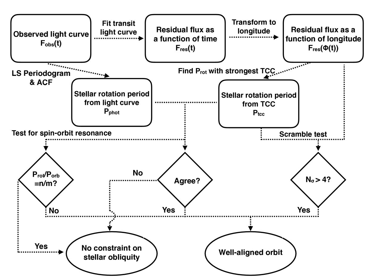
Figure 2.— A flow chart illustrating the major steps in the TCC method.

2.2. Light curve fitting

Figure 2 summarizes the TCC method with a flow chart. We begin with the observed light curve. We isolate the individual transits, retaining only the segments of data spanning twice the transit duration and centered on each transit midpoint. The transit data are used for the TCC computation. The rest of the data are used only to estimate the stellar rotation period. For this purpose we look for the strongest peak in the Lomb-Scargle periodogram of the light curve, and designate this as $P_{\rm phot}$, the photometric rotation period, with an uncertainty equal to the full width at half maximum of the peak. We also estimate the stellar rotation period based on the auto-correlation function (McQuillan et al., 2013, 2014), and consider $P_{\rm phot}$ to be securely measured when the results from the periodogram and the auto-correlation function are in agreement.

We then fit a simple transit model assuming no active regions, and compute the residuals between the data and the best-fitting model. For the model we use the Batman code (Kreidberg, 2015), with the following parameters: the orbital period $P_{\rm orb}$; the planet-to-star radius ratio ($R_{p}/R_{\star}$); the scaled orbital distance ($a/R_{\star}$); the impact parameter ($b\equiv a\cos i/R_{\star}$); the quadratic limb-darkening coefficients ($u_{1}$ and $u_{2}$), the transit midpoint ($t_{0}$); and two coefficients of a quadratic function of time to account for the longer-timescale stellar flux variation near the time of the transit. We adopt the usual $\chi^{2}$ likelihood function and obtained the maximum-likelihood solution using the Levenberg-Marquardt algorithm as implemented in the Python package lmfit (Newville et al., 2014).

After each transit is fitted individually we “rectify” the light curves, dividing the data by the best-fitting quadratic function of time. Then we fit all the rectified light curves together with a reduced set of parameters: $P_{\rm orb}$, $R_{p}/R_{\star}$, $a/R_{\star}$, $b$, $t_{0}$, $u_{1}$ and $u_{2}$.

Next we allow for the possibility of TTVs, and for transit depth variations caused by untransited active regions. When the untransited portions of the star are relatively faint, the loss of light due to the planet increases, and vice versa. We account for these effects by fitting the individual light curves again but with only two adjustable parameters: the time of transit ($t_{0}$), and an additive constant ($\Delta F$) to account for the overall changes in flux of the star. We hold the other parameters fixed at the values determined in the preceding joint fit of all the light curves. The model for the observed transit light curve is then

$$F_{\text{calc}}=\frac{F_{\text{tra}}+\Delta F}{1+\Delta F},$$ (2)

where $F_{\text{tra}}$ is the transit model calculated by Batman and the denominator sets $F_{\text{calc}}=1$ outside of transits, the same normalization that was adopted for the data. To prevent overfitting we require $|\Delta F|$ to be smaller than the observed peak-to-peak variation of the relative flux across the entire light curve. After this final fit to each light curve, we record the residual flux $F_{\text{res}}\equiv F_{\text{obs}}-F_{\text{calc}}$, and transform the time stamps into transit longitude $\Phi$ using Equation 1.

2.3. Searching for Transit Chord Correlations

We are now in the position to seek statistical evidence for the recurring pattern in the residuals that one would expect for a low-obliquity system. First we group together the residuals from a certain number $N_{\rm tra}$ of consecutive transits. The reason for grouping is two-fold: (1) each transit only probes the visible side of the photosphere, and we need at least a few transits to obtain complete longitude coverage; (2) grouping transits together enhances the SNR. The case $N_{\rm tra}$ = 1 corresponds to no grouping. To illustrate the method, Figure 3 shows the data for Kepler-17, a young and active G star with a 1.5-day hot Jupiter. The system was found to have a low obliquity through an earlier application of the spot-crossing method (Désert et al., 2011). Shown are the residuals for five neighboring groups of transits, each of which is composed of five consecutive transits. All five of these groups show a very similar pattern as a function of longitude, as we would expect for a low-obliquity star.

To quantify the significance of the correlations, we perform the following steps. First we bin the residual flux uniformly in transit longitude. We compute normalized residuals,

$$r_{i,j}\equiv\frac{F_{\text{res}}(i,j)}{\sigma_{\text{res}}(j)},$$ (3)

where $F_{\text{res}}(i,j)$ is the median of the residual fluxes in the $i$th group of transits and $j$th bin in transit longitude, and $\sigma_{\text{res}}(i,j)$ is the standard deviation of the residuals of all the data in the $i$th group that contribute to the $j$th bin. Finally, we define the transit chord correlation (TCC) as the average of the dot products of the residuals between neighboring groups:

$${\rm TCC}\equiv\frac{1}{N_{\text{gr}}-1}\sum_{i}^{N_{\text{gr}}-1}\frac{1}{N_{\Phi}}\sum_{j}^{N_{\Phi}}{r_{i,j}\times r_{i+1,j}}$$ (4)

where $N_{\text{gr}}$ is the total number of groups observed, and $N_{\Phi}$ is the number of longitude bins. We selected $N_{\Phi}$ such that each bin contains at least five data points; typically $N_{\Phi}\approx 100$. In some cases, gaps in the data resulted in an empty bin, in which case we set $F_{\text{res}}(i,j)=0$.

Note that the dot products of the residuals are only computed between neighboring groups. This is because each neighboring pair is only separated by a relatively short timescale (a few orbital periods). On longer timescales, we expect the correlation between different groups to dwindle because there might have been enough time for the active regions to undergo substantial evolution or migration. We will see later that Kepler-17 and many other systems do show evidence for evolution of the active regions.

We compute the TCC on a 2-d grid of possible choices for the stellar rotation period $P_{\rm rot}$ and the number $N_{\rm tra}$ of neighboring transits that are included in each group. The stellar rotation period that gives rise to the strongest correlation is denoted as $P_{\text{tcc}}$. For a star with a low obliquity, the strongest TCC should be observed when we calculate the transit longitude using the independently measured stellar rotation period, i.e., for $P_{\rm tcc}=P_{\rm phot}$, within the uncertainties in the observations and the degree of differential rotation. Figure 4 shows the TCC grid for Kepler-17. In this case, $P_{\text{tcc}}=11.8\pm 0.7$ days agrees very well with $P_{\text{phot}}=11.9\pm 1.1$ days, which is good evidence that this star has a low obliquity.

We also need to establish the threshold value of TCC to be considered statistically significant. We do so with a Monte Carlo procedure. In each of $10^{3}$ trials, we scramble the transit epochs, i.e., we randomize the order of the individual transits without affecting the individual light curves. In this way, we remove any correlations between neighboring transits due to spot-crossing events, while preserving the structure of the residuals (the “red noise”) within each transit light curve. For each trial we recalculate the TCC using the values of $P_{\rm tcc}$ and $N_{\rm tra}$ that produced the strongest correlation in the real dataset. We find the resulting distribution of TCC to be nearly Gaussian with a well defined standard deviation, as one would expect from the central limit theorem. The TCC distribution for Kepler-17 is shown in Figure 5. The statistical significance of the TCC of the real data is quantified by the number of standard deviations ($N_{\sigma}$) away from the median of the Monte Carlo distribution.

The final question is, what threshold should be set on $N_{\sigma}$ for a statistically robust detection of correlation? We found that statistical fluctuations alone sometimes produce a TCC with $\text{N}_{\sigma}=$ 2–3 for a random value of $P_{tcc}$ (not necessarily close to $P_{phot}$). This is because when searching for the strongest TCC, we step through a grid of different stellar rotation periods. At each grid point, the transit longitudes and hence the TCC is recomputed with the new rotation period. Typically, we test a rotation period grid with about 200 different periods. It is often the case that a random rotation period among the 200 periods tested produce a 2 or 3-$\sigma$ outlier just by chance. We therefore set a threshold of low-obliquity detection at $\text{N}_{\sigma}>4$. Even more importantly, we guard against spurious detections by requiring that $P_{\rm tcc}$ must agree with $P_{\text{phot}}$.

2.4. The problem of spin-orbit commensurabilities

When the ratio of the stellar rotation period and the planetary orbital period is close to the ratio of small integers, i.e., $P_{\rm rot}/P_{\rm orb}=n/m$, then the planet and the star return to the same sky-projected configuration every $n$ orbital periods or $m$ rotation periods. Such a spin-orbit commensurability may be the result of a physical process that drove a system into a spin-orbit resonance, or may simply occur by chance. Upon returning to the same sky-projected configuration, the planet will occult the same set of active regions. The TCC will therefore be strong regardless of the stellar obliquity. Fortunately, these cases for which the TCC is blind to obliquity can be easily recognized because $P_{\rm phot}$ and $P_{\rm orb}$ are both known in advance. Moreover, in such cases, the TCC will usually be strongest at $P_{\rm tcc}=mP_{\rm rot}=nP_{\rm orb}$, rather than $P_{\rm rot}$.

In practice, our code raises an alarm whenever $P_{\rm phot}/P_{\rm orb}$ falls within 5% of a ratio of small numbers and $P_{\text{tcc}}$ also falls within 5% of $nP_{\rm orb}$. In these cases, we carry out a visual inspection of the light curve, which can easily distinguish the low-obliquity from the high-obliquity cases: in the low-obliquity case spot/faculae crossing events recur in all neighboring transits; whereas in the high-obliquity case spot/faculae crossing events only recur after $nP_{\rm orb}$.

In summary, we declare a statistically significant detection of low stellar obliquity if the system satisfies: (1) $P_{\text{tcc}}$ agrees with $P_{\text{phot}}$ to within the uncertainties; (2) $N_{\sigma}>4$; and (3) the orbital and rotation periods are not in the ratio of small integers. For such systems we can place an upper bound on the allowed obliquity using a simple geometric argument. Between consecutive transits, the active regions move through an angle of $2\pi/P_{\text{rot}}\times P_{\text{orb}}$. The angular displacement of the active region between consecutive transits is therefore

$$\Delta\theta=~{}{\rm mod}(\frac{2\pi P_{\text{orb}}}{P_{\text{rot}}},2\pi).$$ (5)

In a well-aligned system, the active regions move along the transit chord, along the $x$ direction. However a non-zero obliquity introduces a vertical motion, in the $y$ direction. In order to observe a recurring pattern, the active regions must remain within the transit chord for at least two transits. For this to happen the vertical motion of the active regions must be smaller than the width of the transit chord,

$$\Delta\theta\times\text{sin}(\Psi)\lesssim\frac{R_{p}}{R_{\star}}.$$ (6)

For giant planets around Sun-like stars this leads to a typical upper limit of 10^∘, though it is only approximate because we have neglected the effects of the stellar inclination toward or away from the observer. Also, in cases where the active regions are larger than the planet radius, we should replace $R_{p}/R_{\star}$ by the size of the active regions relative to the star.

To allow a visual inspection of all the data we introduce the “transit tapestry”, shown in the left panel of Figure 6 for Kepler-17. This is a heat map in which the color scale represents the residual flux, the horizontal dimension is transit longitude, and the vertical dimension is the transit group number (essentially, the time). If a star has a low obliquity, then long-lived and stationary active regions will appear as vertical features in the image. Evolution of the active regions will cause the features to vary slowly in the vertical direction, and migration in longitude will cause them to vary in the horizontal direction. These effects produce a tapestry-like pattern of coherent features, which displays the properties of the active regions such as their sizes, relative intensities, lifetimes and migration patterns. If the obliquity is large or the active regions are weaker then the image will lose its artistic appeal and look like random static, as in the right panel of Figure 6, which was generated after scrambling the transit epochs.

2.5. Retrograde Orbits

Although our emphasis in this description has been on the detection of low-obliquity orbits, it is worth noting that the same method can just as easily be used to identify planets on nearly perfectly retrograde orbits ($\Psi=180^{\circ}$). This is because the transit chord of a retrograde-orbiting planet is also parallel to the lines of latitude on the stellar photosphere. In such a geometry, active regions on the star can be occulted multiple times in neighboring transits and produce strong correlations in the residual flux. To search for retrograde systems, we simply flip the sign of the second term in Equation 1 and proceed again with all the other steps in the analysis.

In fact it is not strictly necessary to perform two completely different analyses, one for prograde and the other for retrograde systems. Even if the positive sign is always retained in Equation 1, a retrograde system will distinguish itself by producing a strong TCC for a value of $P_{\rm tcc}$ that is not equal to the stellar rotation period, but rather at the period given by

$$\frac{1}{P^{\prime}_{\rm tcc}}=\frac{1}{P_{\rm orb}}-\frac{1}{P_{\rm rot}}.$$ (7)

This is because in between two transits, the active regions on a retrograde star with rotation period $P^{\prime}_{\rm tcc}$ will rotate through the same angle as a prograde star with rotation period $P_{\rm rot}$. In general $P^{\prime}_{\rm tcc}$ differs significantly from $P_{\rm rot}$. The only exception is the case $P_{\rm rot}$ = 2$P_{\rm orb}$, which is already handled in the test for spin-orbit commensurabilities.

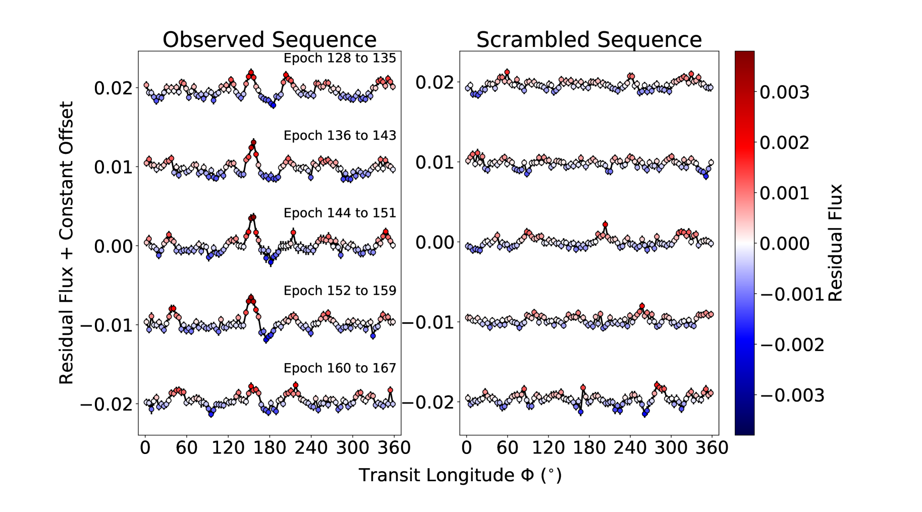
Figure 3.— Residual fluxes for Kepler-17b. The colored circles show the binned residual flux as a function of transit longitude. As in Figure 6, positive residuals are red and negative residuals are blue. The left panel shows data from five consecutive groups of transits. Each group consists of eight transits, which together provide complete longitude coverage from 0 to 360^∘. A coherent pattern recurs from one group to the next. This is indicative of a low-obliquity orbit, as illustrated in Figure 1. The right panel shows the same dataset after scrambling the epoch numbers of the transits. No recurring pattern is seen.

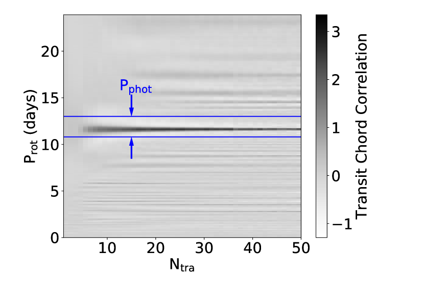
Figure 4.— Transit Chord Correlation (TCC) for Kepler-17b, as a function of $P_{\text{rot}}$, the rotation period that is assumed when computing transit longitudes, and $N_{\rm tra}$, the number of transits per group. The blue lines show the 1-$\sigma$ confidence interval in the measurement of $P_{\text{phot}}$, the stellar rotation period based on the photometric periodicity in the out-of-transit light curve. The strongest TCC occurs at $P_{\text{tcc}}=11.8\pm 0.7$ days which agrees well with $P_{\text{phot}}=11.9\pm 1.1$ days. This agreement is strong support for the claim that the recurring pattern we see in Figure 3 is due to active regions on a low-obliquity host star.

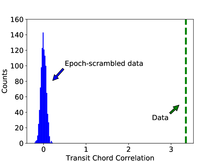
Figure 5.— Statistical significance of the TCC for Kepler-17b. To quantify the statistical significance of the recurring pattern seen in Figure 3 and 6, a scrambling test is conducted. We recompute the TCC after randomizing the epoch numbers of the individual transits. The resultant distribution is plotted as the blue histogram. The TCC computed with the correct epoch sequence (shown in green) is much stronger than when computed for the scrambled sequences.

3. Sample Selection

We tried to assemble a collection of all the transit datasets for which there seemed to be a reasonable chance of success for the TCC method. The requirement for high SNR and a large number of consecutive transits restricts us to data from the space missions CoRoT, Kepler, and K2.

We included all 29 confirmed CoRoT systems in our sample. We downloaded the light curves from the CoRoT N2 public archive. We used the monochromatic flux labelled “whiteflux” in the FITS header. We only retained data points with a Quality Flag of 0, i.e., those not affected by various known problems.

Analyzing all of the thousands of Kepler Objects of Interest (KOIs) would have required too much computation time. Instead, we selected a sample of confirmed planets, planetary candidates, and eclipsing binaries with high SNR and for which there was some indication of spot-crossing anomalies. The SNR was calculated as the ratio between the transit or eclipse depth and the tabulated 6-hour CDPP (combined differential photometric precision). We identified the 360 KOIs with a single-transit SNR $>$ 20. Evidence for anomalies is based on the ratio of the standard deviation of the photometric residuals during the transit $\sigma_{\rm in}$, and the standard deviation of the out-of-transit data $\sigma_{\rm out}$. Stellar activity should cause this ratio to be significantly larger than unity. We retained the high SNR systems that also have $\sigma_{\rm in}/\sigma_{\rm out}>1.7$. A list of such systems had been compiled by Sanchis-Ojeda (2014). We also included any Kepler systems for which the stellar obliquity had been previously measured using spot-crossing anomalies or any other method. We downloaded the light curves from the MAST website using the Python package kplr . Whenever possible we used the short-cadence light curves, with one-minute time sampling. We used the light curves based on SAP (simple aperture photometry), and we only kept data points with a Quality Flag of 0.

Our sample also includes nine stars with confirmed planets that were observed in the short-cadence mode during the K2 mission (Howell et al., 2014). These systems are HATS-9, HATS-11, Qatar-2, WASP-47, WASP-55, WASP-75, WASP-85, WASP-107 and WASP-118. To produce the light curves, we downloaded the pixel files from the Mikulski Archive for Space Telescopes website (MAST). To remove the spurious intensity fluctuations caused by the uncontrolled rolling motion of the Kepler spacecraft, we used the photometry pipeline described by Dai et al. (2017), which decorrelates the flux variations against the measured coordinates of the center of light on the detector.

The resultant sample consists mainly of FGK dwarf stars, except for Kepler-13A (an A star) and Kepler-45 (an M dwarf). Because of the SNR requirement, the planets in our sample are almost all hot Jupiters. Three-quarters of the planets are larger than $8~{}R_{\oplus}$ and have orbital periods shorter than 10 days. We believe the resulting sample is fairly exhaustive, in the sense that it includes all of the data currently available for which the TCC method has a significant chance of revealing the obliquity. However, the sample is strongly biased toward close-in giant planets around active stars. It is not “complete” in any other sense, i.e., it is not amenable to any simple astrophysical description. Caution is therefore needed when trying to interpret the fraction of systems that are found to be aligned, retrograde, or indeterminate.

4. Results

Tables 1 and LABEL:tab:eb summarize the results for the transiting planets and eclipsing binaries respectively. For each system we report the orbital period ($P_{\text{orb}}$); the scaled semi-major axis ($a/R_{\star}$); the mass and radius of the planet and the host star ($M_{p}$, $R_{p}$, $M_{\star}$, and $R_{\star}$); the effective temperature of the host star ($T_{\text{eff}}$); the rotation period measured from the quasiperiodic modulation in the light curve ($P_{\text{phot}}$); the rotation period that gives the strongest TCC ($P_{\text{tcc}}$); the statistical significance of the correlation based on the scrambling test ($N_{\sigma}$); the ratio between the rotation and orbital periods ($P_{\text{tcc}}/P_{\text{orb}}$); and any previous measurement of the sky-projected obliquity that has appeared in the literature $\lambda_{\text{lit}}$. We have arranged the table such that systems that show statistically significant TCC (those with a low stellar obliquity) appear in front. For those systems we report an upper limit on the true obliquity using Equation 6. The other systems are arranged in descending order of $N_{\sigma}$.

To check on the validity of the TCC method, we examined the results for all the systems for which stellar obliquities had been measured with other methods. For the low-obliquity systems (those that satisfy Equation 6), we may detect a strong TCC with $P_{\text{tcc}}=P_{\text{phot}}$. However, a null result could also be obtained, if the host star is not sufficiently active, the planet’s transit chord misses the active latitudes, or the active regions undergo rapid evolution. Therefore we began by focusing on the low-obliquity systems where previous studies had revealed strong stellar activity through the clear identification of individual spot-crossing events: Kepler-17 (Désert et al., 2011), CoRoT-2 (Nutzman et al., 2011) and Qatar-2 (Močnik et al., 2016b; Dai et al., 2017). These are hot Jupiters around active G or K stars, with orbital periods less than two days. For all of these systems, individual spot-crossing anomalies could be visually identified in the light curves. The recurrence of the spot-crossing events led previous authors to conclude that all three systems are aligned to within $\approx$$10^{\circ}$. Additionally, for the case of Qatar-2b, Esposito et al. (2017) found $\lambda=0\pm 10^{\circ}$ based on the Rossiter-McLaughlin effect. Unsurprisingly, these three systems show the strongest TCC among all the systems in our sample, and $P_{\rm tcc}$ agrees well with $P_{\rm phot}$. Thus the TCC method easily confirms the low stellar obliquities for these systems.

Holczer et al. (2015) reported five systems with prograde obliquities (Kepler-17b, Kepler-71b, KOI-883.01, KIC 7767559b and Kepler-762b), based on the observed correlation between the apparent TTV and the local time derivative of the out-of-transit flux. This method was described in the Section 1. The TCC method shows that the orbits of all five systems are not only prograde ($\Psi<90^{\circ}$) but also aligned to within about $\Psi\lesssim 10^{\circ}$.

We now turn to the eight systems for which other methods unveiled a high stellar obliquity (see Table 1 for the measured obliquities and references). For CoRoT-3b, CoRoT-19b, Kepler-13Ab, Kepler-420b, HAT-P-7b, and WASP-107b, we did not detect a statistically significant TCC. For those cases in which the stellar rotation period could be measured from the light curve, $P_{\text{phot}}$ did not agree with $P_{\text{tcc}}$. This is as expected, for high-obliquity systems. However, our method did return a statistically significant TCC for the HAT-P-11b and Kepler-63b systems, which are known to be misaligned (Sanchis-Ojeda & Winn, 2011; Sanchis-Ojeda et al., 2013). We found $N_{\sigma}=6.0$ for HAT-P-11b and 5.8 for Kepler-63b. These “false positives” are examples of the problem of spin-orbit commensurability described in the previous section. Béky et al. (2014a) reported a 6:1 spin-orbit period ratio for HAT-P-11b, and Sanchis-Ojeda et al. (2013) reported a nearly 4:7 ratio for Kepler-63b. The strongest TCC for Kepler-63 was detected at $P_{\text{tcc}}=37.7$ days (4$\times P_{\text{orb}}$) rather than $P_{\rm phot}$ = 5.401$\pm 0.014$ days.

After completing the search for well-aligned systems, we used the same sample to search for perfectly retrograde systems. We flipped the sign of the second term in Equation 1 before repeating the TCC analysis. We did not find any cases of a statistically significant TCC. Hence, although we could have detected perfectly retrograde orbits just as easily as we detected prograde orbits, we did not find any evidence for perfectly retrograde orbits in our sample. In the following sections we discuss some of the individual systems in greater detail.

4.1. Kepler-17

Kepler-17b is a hot Jupiter orbiting a G star every 1.5 days. Désert et al. (2011) identified and modeled a sequence of spot-crossing events in neighboring transits. The recurrence of the spot-crossing events led Désert et al. (2011) to conclude that the Kepler-17b has an obliquity ¡ 15^∘. Our analysis revealed a strong TCC ($N_{\sigma}$ = 59.6) at $P_{\text{tcc}}=11.8\pm 0.7$ days. The Kepler light curve shows rotational modulation in the out-of-transit light curve which offers an independent check on the stellar rotation period: $P_{\text{phot}}=11.9\pm 1.1$ days. These observations together suggest a low stellar obliquity of Kepler-17b; and we place an upper bound $\Psi\lesssim$ 10^∘ with Equation 6.

Figure 6 shows the transit tapestry for Kepler-17. It displays clear clusterings of positive and negative residuals in transit longitude. We interpret the observed clustering as photometric signatures of active regions along the transit chord. These patterns can be used to infer the properties of the host star’s magnetic activity. At any particular time there are 1–4 active regions present on the transit chord. Each of these regions in the tapestry spans 20–30^∘ in transit longitude. However, the nonzero size of the the planet (about 16^∘ in longitude) acts to widen the apparent size of the active regions. After accounting for the size of the planet, the active regions span 5–20^∘ in true longitude on the star. The active regions lasted for a 100–200 days before either disappearing or leaving the latitudes probed by the planet. The intensity of the active regions changed gradually over time; they did not burst into existence with maximum intensity.

One point of interest is whether the active regions remain stationary in longitude or undergo longitudinal migration. However, there is a degeneracy between any constant rate of longitudinal migration, and the rotation period used to calculate transit longitudes. Specifically, if $P_{\rm tcc}$ is smaller than the actual stellar rotation period, all the photometric features in the transit tapestry would appear to undergo prograde longitudinal migration in the transit tapestry. The TCC method, by design, maximizes the correlation of residual flux. As a result, it always selects the stellar rotation period such that most photometric features remain fixed in stellar longitude. Therefore, the transit tapestry can only reveal relative migration rates between different active regions but not the absolute rate of migration. In the case of Kepler-17, there is indeed some indication of relative migration. The pattern enclosed by the green ellipse in Figure 6 suggests that an active region split apart into two smaller regions which separated longitudinally over time. This is reminiscent of the emerging magnetic flux tubes on the Sun which produce bipolar magnetic regions (Spruit & Roberts, 1983). A flux tube initially gives rise to one footpoint on the host star when it just reaches the stellar surface. As the flux tube emerges further, it gives rise to two footprints that spread apart in longitude.

From now on, we will define the contrast of an active region as the relative ratio between the brightness of the active regions to the average photosphere, in the observing bandpass. Specifically for Kepler-17, the photometric features of the active regions had amplitudes of about 0.002–0.004 in relative flux. By comparing this to the transit depth of about 0.02, the active regions on average are seen to be roughly 10-20% fainter than the average photosphere in the broad optical Kepler bandpass (approximately 420–900 nm). We note that the finite size of the transiting planet introduces a convolution effect that not only broadens the photometric signature of the active regions, but also reduces the contrast. The contrast calculated here and subsequently is the product of the relative brightness of individual magnetic features that constitute the active regions and the area filling factor within the shadow of the planet. Because of this degeneracy, we refrain from converting the contrast into an effective temperature (which would have allowed for more direct comparisons with sunspots).

Figure 6 shows that the number, size, and relative intensity of active regions decreased towards the latter part of the Kepler mission. This decline might have been part of a magnetic activity cycle, or it might represent the latitudinal migration of the active regions away from the transit chord. In principle, the degree of differential rotation could be studied by comparing the rotation period on the transit chord $P_{\text{tcc}}$ with the photometrically-derived rotation period $P_{\rm phot}$, which is based on active regions across the entire star. However, this is difficult in practice because there is little information on how the active regions are distributed latitudinally outside the transit chord. Given the impact parameter of the transit $b=0.27$ (Désert et al., 2011) and the size of the planet $R_{p}/R_{\star}\approx$0.13, the stellar latitude probed by the planet is $16\pm 8^{\circ}$ north or south of the stellar equator. At least, our analysis can show that this latitudinal range is magnetically active.

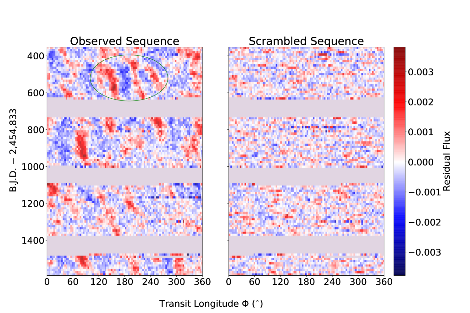
Figure 6.— Transit Tapestry of Kepler-17b. The residual flux of Kepler-17b as a function of transit longitude and time. Red indicates positive residuals, and blue indicates negative residuals. A portion of these data (BJD 540–600) are shown in Figure 3. The coherent and generally vertical patterns imply a low stellar obliquity. These patterns allow for estimates of some key properties of the active regions, including size (5–20^∘ in longitude), lifetime (100–200 days), and relative intensity (10–20% dimmer than average photosphere). Some active regions are observed to split into two smaller active regions (see, e.g., the green ellipse). We interpret this as the result of emerging magnetic flux tubes. For comparison, the right panel shows the transit tapestry for a scrambled dataset, in which the transit epochs were randomized.

4.2. CoRoT-2

CoRoT-2b is a hot Jupiter orbiting a G star every 1.7 days (Alonso et al., 2008). The star rotates rapidly, with a period of about 4.5 days, and has strong magnetic activity which manifested as clear spot-crossing events in the CoRoT light curve. By modeling the recurrence of spot-crossing events, Nutzman et al. (2011) found the sky-projected obliquity to be $\lambda=4.7\pm 12.3^{\circ}$. Our TCC method tells a consistent story. We find a strong TCC $N_{\sigma}$ = 22.6 at $P_{\text{tcc}}=4.5\pm 0.3$ days consistent with $P_{\text{phot}}$ of $4.530\pm 0.068$ days. We conclude that CoRoT-2 has a low stellar obliquity

Figure 7 shows the transit tapestry. The clustering of residual flux indicates that there were two active regions present on the stellar latitude probed by the planet. They had similar sizes and intensities and were separated by about $180^{\circ}$ in longitude. These two regions span about 30–40^∘ in the transit tapestry. After accounting for the blurring effect of the planet, which extends about 20^∘ in longitude, we conclude the active regions are about 10-20^∘ wide. Both active regions persisted throughout the $\approx$150 days of CoRoT observations, remaining nearly stationary in longitude. With Figure 7, we can estimate that active regions produce flux variation of about 0.002–0.005 in relative flux. Taking the ratio with the transit depth (about 3%), we find the active regions to be roughly 7-17% dimmer than the rest of the photosphere in the CoRoT bandpass. Again, using the impact parameter of the transit $b\approx 0.22$ (Gillon et al., 2010a) and the size of the planet $R_{p}/R_{\star}\approx 0.13$, the stellar latitude probed by the planet is likely $13\pm 10^{\circ}$ in either the northern or southern hemisphere.

Lanza et al. (2009) and Huber et al. (2010) also studied the magnetic activity of CoRoT-2. Lanza et al. (2009) used a maximum entropy method to determine the longitudinal distribution of active regions using the rotational modulation in the out-of-transit light curve, while Huber et al. (2010) modeled the transit light curve by dividing the eclipsed and noneclipsed parts of photosphere into a number of longitudinal intervals with different intensities. Both of these works confirmed the presence of active regions on CoRoT-2.

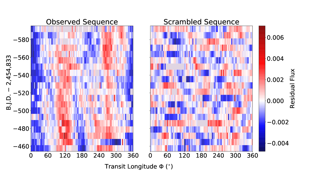
Figure 7.— Transit Tapestry of CoRoT-2b. Same as Figure 6 but for CoRoT-2. The TCC method makes a strong case for a low stellar obliquity. In contrast to Kepler-17, there appear to be two active regions along the stellar latitude probed by the planet. They have similar intensity (7-17% dimmer than average photosphere) and size (10-20^∘ in longitude); and are located rather symmetrically on opposite hemispheres. The active regions persisted throughout the $\approx$150 days of CoRoT observations. The transit chord of CoRoT-2b correspond to a stellar latitude of $13\pm 10^{\circ}$.

4.3. Qatar-2

Qatar-2b is a hot Jupiter discovered by the Qatar Exoplanet Survey (Bryan et al., 2012). The planet orbits a K dwarf every 1.3 days. Recent K2 observations in the short-cadence mode unveiled dozens of spot-crossing anomalies. By modeling the spot-crossing anomalies, both Močnik et al. (2016b) and Dai et al. (2017) showed that the system has a low stellar obliquity. Esposito et al. (2017) independently confirmed the low stellar obliquity $\lambda=0\pm 10^{\circ}$ by observing the Rossiter-McLaughlin effect. As expected, we detect a strong TCC $N_{\sigma}$ = 18.0 in the K2 light curve at $P_{\text{tcc}}=18.2\pm 0.4$ days which agrees with $P_{\text{phot}}$ = $18.5\pm 1.5$ days. We place an upper bound $\Psi\lesssim 11^{\circ}$.

Figure 8 shows the tapestry plot for Qatar-2. Although K2 observations only spanned 80 days, the transit tapestry still reveals two active regions along the transit chord. One of them was located at 300^∘ in longitude and was about 15–25^∘ wide (after accounting for the broadening due to the nonzero size of the planet). Its intensity remained relatively constant throughout the 80 days of K2 observations. The other active region was located near 20^∘ in longitude. Its size and intensity underwent a significant increase during the K2 observation. This might have been caused by the emergence of a magnetic flux tube, or latitudinal migration of an active region into the transit chord. These active regions maintained a constant separation in longitude. The active regions on average are roughly 3-7% dimmer than the photosphere. Given the impact parameter of the transit $b\approx 0.03$ (Dai et al., 2017) and $R_{p}/R_{\star}=0.15$, the transits probe the region close to the stellar equator ($2\pm 9^{\circ}$).

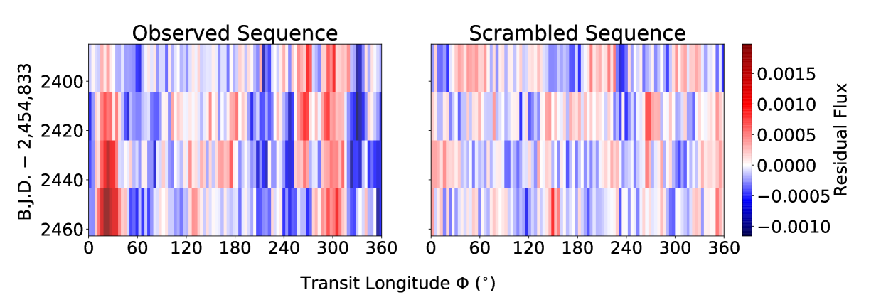
Figure 8.— Transit Tapestry of Qatar-2b. Same as Figure 6 but for Qatar-2. TCC analysis reveals a low stellar obliquity. One of the active regions was located at 300^∘ in longitude. Its intensity remained relatively constant during the 80 days of K2 observation. The other active region was located near 20^∘ in longitude. Its size and intensity underwent significant increase during the K2 campaign.

4.4. Kepler-71

Kepler-71b is a 3.9-day hot Jupiter around a G star (Howell et al., 2010). With a V magnitude of 15.4, Kepler-71 is too faint for precise radial-velocity follow-up. Holczer et al. (2015) detected a strong correlation between the detected TTV and the time derivative of the stellar flux, which suggested a prograde orbit and the presence of starspots. Our TCC analysis shows that the orbit of Kepler-71b is not only prograde but also well-aligned. We detect a strong TCC ($N_{\sigma}$ = 10.7; $P_{\text{tcc}}=19.7\pm 0.8$ days; $P_{\text{phot}}$ = $19.87\pm 0.18$ days). The upper bound on the obliquity is $\Psi$ $\lesssim$ 6^∘.

We made a transit tapestry for Kepler-71 (Figure 9). Two active regions are most discernible in the later part of the Kepler mission (BJD-2454833 ¿ 1200). These two active regions were separated by about 180^∘. They each spanned about 5-15^∘ in longitude after accounting for the convolution effect of the planet (16^∘ in longitude). They lasted for about 150 days; and on average were roughly 10-20% dimmer than the photosphere. We estimate the latitude probed by the planet using the impact parameter of the transit (0.04, Howell et al., 2010) and the size of the planet ($R_{p}/R_{\star}\approx$ 0.14). The result shows that the equatorial region of the photosphere ($2\pm 8^{\circ}$) is magnetically active.

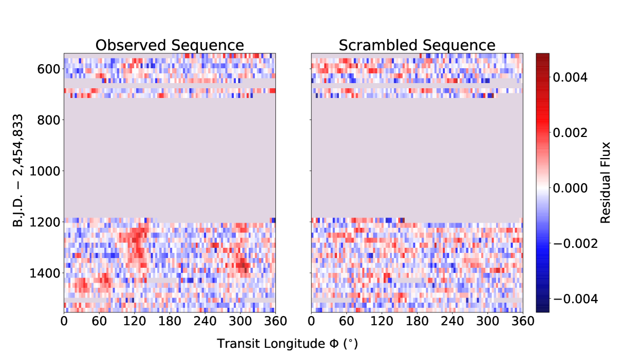
Figure 9.— Transit Tapestry of Kepler-71b. Same as Figure 6 but for Kepler-71. TCC detects a strong correlation consistent with a low stellar obliquity. Two large-scale active regions emerged in the later part of the Kepler mission. The active regions were separated by about 180^∘. They each spanned about 5-15^∘in longitude. They have similar lifetime ($\sim$ 150 days) and relative intensity (10-20% dimmer than average photosphere). Given its impact parameter, the planet probes the equatorial region ($2\pm 8^{\circ}$ in latitude).

4.5. KOI-883.01

KOI-883.01 is a planetary candidate discovered by the Kepler mission. The transit light curve is consistent with a hot Jupiter orbiting a K star every 2.7 days. As was the case with Kepler-71, Holczer et al. (2015) detected a strong correlation between TTV and local flux variation and inferred a prograde orbit for the system. We show that the system is not only prograde but also well-aligned. The $N_{\sigma}$ is as high as 9.2 while $P_{\text{tcc}}=9.1\pm 0.2$ days and $P_{\text{phot}}=9.11\pm 0.11$ days agree well. We place an upper bound $\Psi$ $\lesssim$ 4^∘.

The transit tapestry is shown in Figure 10. The photometric signatures of active regions are more diffuse than for the systems described earlier. In the first $\approx$100 days of Kepler observations, an active region was located near 240^∘ in longitude and was 20–30^∘ wide (after accounting for the 18^∘ angular size of the planet). After a gap in the data, another active region emerged at 120^∘ in longitude with a similar size and intensity (10-20% dimmer than the average photosphere). Both active regions lasted for at least 100–200 days, and perhaps even longer if the active region near 240^∘ persisted through the data gap. The impact parameter of the transit is about 0.01 and $R_{p}/R_{\star}$ is about 0.18 (ExoFoP ). The transit chord overlaps with the equatorial region ($0\pm 10^{\circ}$) which appears to be magnetically active.

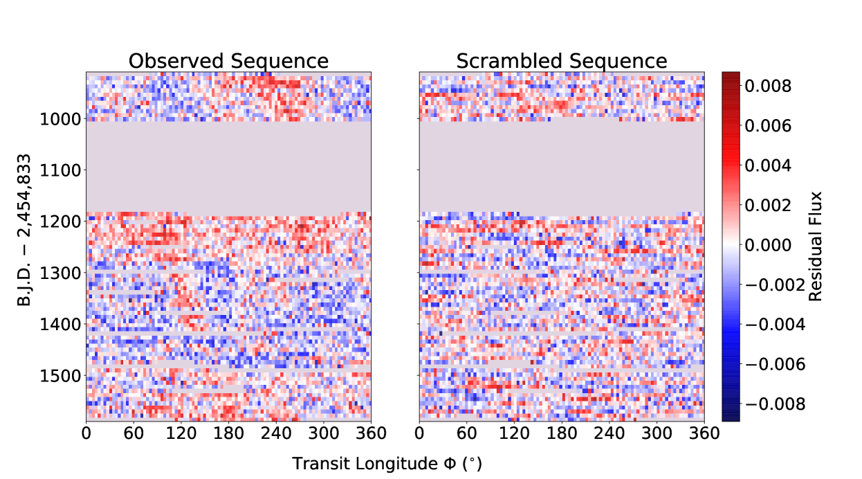
Figure 10.— Transit Tapestry of KOI-883.01 Same as Figure 6 but for KOI-883. TCC analysis revealed a low stellar obliquity. An active region was located at 240^∘ in longitude during the first 100 days of Kepler observation. The second active region emerged near 120^∘ in longitude with similar width (20-30^∘ in longitude) and intensity (10-20% dimmer than the average photosphere) after the data gap of about 200 days.

4.6. Kepler-45

Kepler-45b is a 2.5-day hot Jupiter orbiting a M dwarf. The system was confirmed by a combination of radial velocity monitoring, adaptive optics imaging, and near-infrared spectroscopy (Johnson et al., 2012). It is one of the three hot Jupiters around M dwarfs that have been reported to date. The other two are HATS-6b (Hartman et al., 2015) and NGTS-1b (Bayliss et al., 2017). No constraint on the stellar obliquity of Kepler-45b has been published yet.

Application of the TCC method gave $N_{\sigma}$ = 6.3 at $P_{\text{tcc}}=16.7\pm 0.8$ days. The $P_{\text{tcc}}$ coincides with the measured $P_{\text{phot}}$ = $15.8\pm 0.2$ days, to within the uncertainties. We conclude that Kepler-45b is very likely on a well-aligned orbit, with an upper bound on $\Psi$ $\lesssim$ 11^∘. To our knowledge, this is only the second case of a stellar obliquity measured for an M dwarf. The first such report was for GJ 436b, a 2.6-day Neptune-mass planet (Bourrier et al., 2017, $\lambda=72^{+33}_{-24}~{}^{\circ}$). Enlarging the number of such measurements would be interesting. Being fully convective, some M-dwarfs are structurally very different from solar-type stars for which most of the obliquity measurements have been obtained. The excitation and damping of stellar obliquities may operate in different ways for M dwarfs than for solar-type stars. Given that other, more traditional obliquity measurements tend to fail for M dwarfs, the TCC method may be particularly promising for constraining the stellar obliquities of M-dwarf planet hosts. We will return to this point in Section 5.

Kepler-45b has an impact parameter of about 0.6 (Johnson et al., 2012) and a $R_{p}/R_{\star}$ of 0.18. Together this suggests that the transit chord probes the stellar latitude of $37\pm 16^{\circ}$. The transit tapestry, shown in Figure 11, does not show any visually compelling patterns. This is because we have organized this section in order of decreasing correlation strength. At this point, the correlations may not be visually obvious, even though our Monte Carlo procedure shows that they are statistically significant when summed over the entire dataset. Alternatively, it may be the case that active regions on M-dwarfs preferentially take the form of broad chromospheric plages and networks rather than dark photospheric spots on sun-like stars. The resultant photometric features in the transit light curves would be more spread out, more rapidly evolving and hence harder to discern visually, compared to the sun-like stars described earlier. The increased chromospheric activity of M dwarfs was observed in Ca II H and K lines (Isaacson & Fischer, 2010). Moreover, the difference in magnetic behavior between M dwarfs and solar-type stars is also theoretically motivated: fully convective M dwarfs lack the tachocline, the strong shearing zone between the radiative and convective layer of the sun, which is thought to be important for the operation of sun-like dynamos and the formation of sunspots (Charbonneau, 2014).

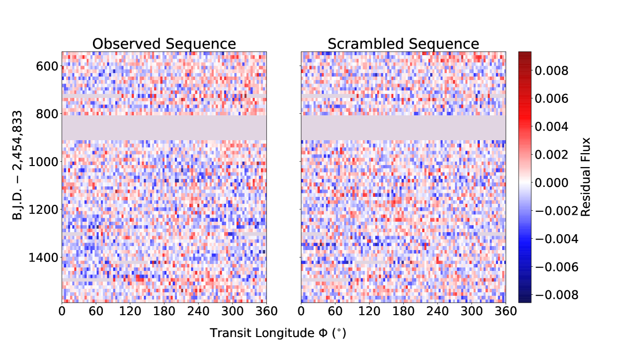
Figure 11.— Transit Tapestry of Kepler-45b Same as Figure 6 but for Kepler-45. Our TCC analysis suggests a low stellar obliquity. However, any presence of magnetically active regions is not visually obvious. This may be attributed to the low SNR of the light curve. Another possibility is that magnetically activity of the M dwarfs is dominated by bright chromospheric plages/networks instead of dark photospheric spots. The chromospheric features may have much larger areas, less well-defined shapes and shorter lifetimes than the spots. As a result, their photometric features in the transit light curves are harder to discern visually.

4.7. TrES-2

TrES-2 is a G star hosting a 2.5-day hot Jupiter (O’Donovan et al., 2006). Rossiter-McLaughlin observations have shown that TrES-2b has a low stellar obliquity $\lambda=-9\pm 12^{\circ}$ (Winn et al., 2008), although the confidence in that measurement was lower than usual because of the star’s relatively low rotation velocity. We find a strong TCC $N_{\sigma}$ = 5.8 in the residual flux at $P_{\text{tcc}}=29.9\pm 1.4$ days. This period is in agreement with the independently measured photometric period, $P_{\text{phot}}=28.35\pm 0.34$ days. We conclude that TrES-2 likely has a low stellar obliquity with an upper bound $\Psi$ $\lesssim$ 10^∘.

We show the transit tapestry in Figure 12. We can see correlations between neighboring groups, but not any distinct, long-lasting features of the type that appeared in some of the systems described earlier. According to Montet et al. (2017), the photometric activity of solar-type stars with rotation periods greater than 25 days are more likely to be dominated by bright patches (faculae) than by dark spots. These bright patches and the active network, at least those on the Sun, are more extended and evolve more quickly than spots (Foukal, 1998; De Pontieu et al., 2006; Shapiro et al., 2016). Given the slow stellar rotation period of TrES-2, we may be seeing the more extended and less persistent photometric features of the faculae or active networks. In particular, the blue patch spanning about $180^{\circ}$ near BJD-2454833 = 1000 may be associated with a bright, more extended active region.

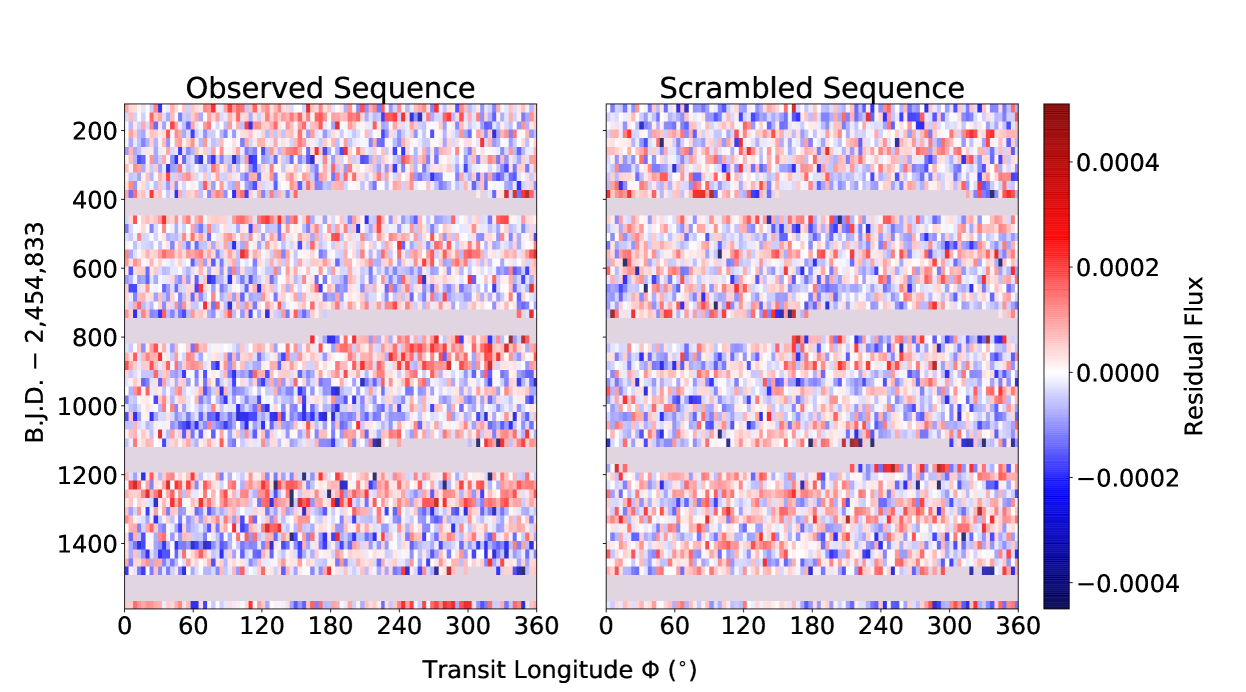
Figure 12.— Transit Tapestry of TrES-2b Same as Figure 6 but for TrES-2. TCC makes a good case for a low stellar obliquity of TrES-2. With a slow stellar rotation of about 29 days, TrES-2 may be dominated by faculae and active networks. The blue patch with transit latitude between 60 and 240^∘ near BJD-2454833 = 1000 may be caused by a bright, extended active region on TrES-2.

4.8. Kepler-762

Kepler-762b is a 3.8-day hot Jupiter around a G star. The planet went from being a “candidate” to being “validated” through the statistical analysis of Morton et al. (2016). Holczer et al. (2015) reported a prograde orbit for this system given the observed strong correlation between TTV and local flux variation. Our TCC analysis shows a good agreement between $P_{\text{tcc}}=4.0\pm 0.1$ days and $P_{\text{phot}}$ = $4.045\pm 0.025$ days. The statistical strength of the correlation is $N_{\sigma}$ = 5.2. We thus argue that the orbit of Kepler-762 is not only prograde but also well-aligned ($\Psi$ $\lesssim$16^∘). The transit tapestry, Figure 13, is not impressive to the eye, even though the TCC is strong enough for a confident conclusion. Given the impact parameter of the transit of about 0.05 (ExoFop) and $R_{p}/R_{\star}$ of 0.10, the transit chord probes the stellar latitude of $3\pm 7^{\circ}$.

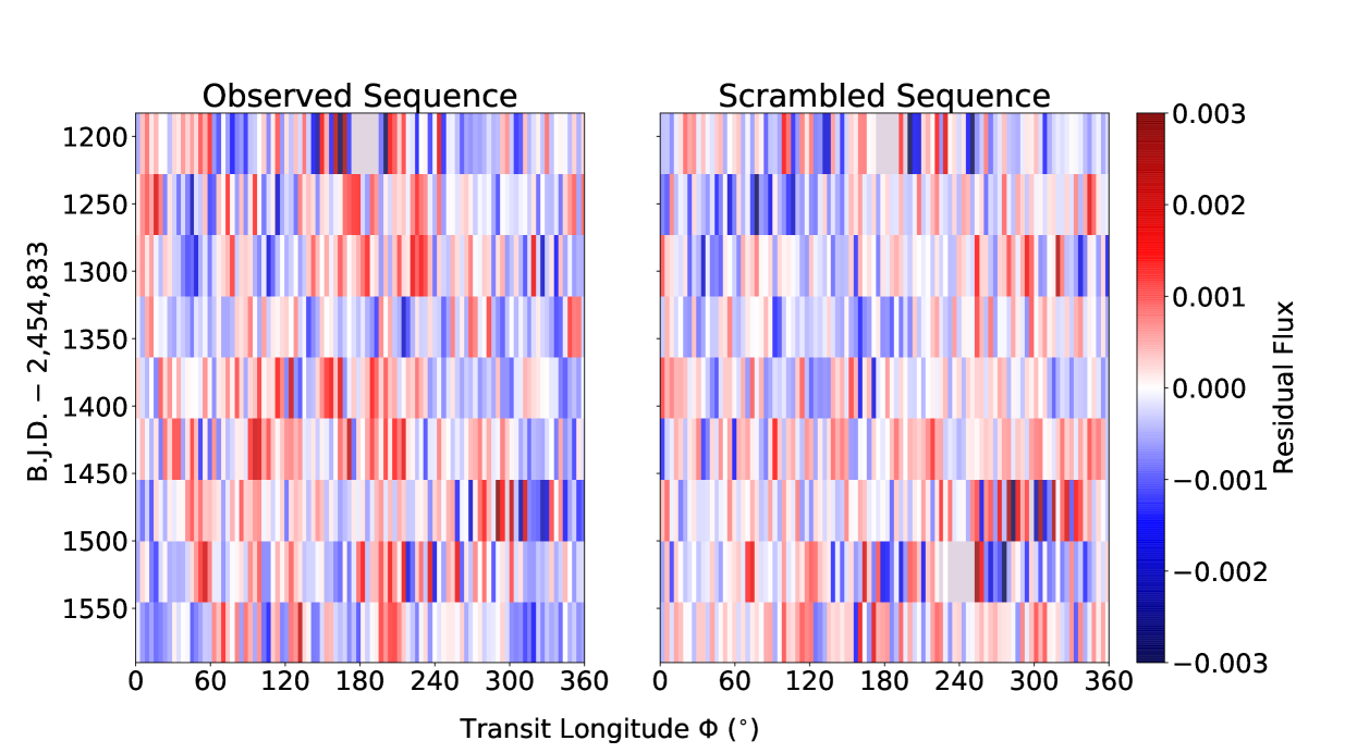
Figure 13.— Transit Tapestry of Kepler-762b Same as Figure 6 but for Kepler-762. A strong correlation was detected by the TCC method suggesting a low stellar obliquity. The presence of active regions is not visually obvious.

4.9. Kepler-423

Kepler-423b is a 2.7-day hot Jupiter orbiting a G star (Gandolfi et al., 2015). The maximum TCC has $N_{\sigma}=4.7$ at $P_{\text{tcc}}=23.0\pm 0.9$ days. The stellar rotation period was also independently measured to be $P_{\text{phot}}$ = $22.047\pm 0.121$ days based on the out-of-transit light curve. Therefore Kepler-762 likely has a low stellar obliquity ($\Psi$ $\lesssim$ 10^∘). In the transit tapestry (Figure 14), there are hints of group-group correlations, however no large-scale, long-lasting active regions can be discerned by eye. As we said with regard to TrES-2, Kepler-423 may be also faculae-dominated given its slow stellar rotation period.

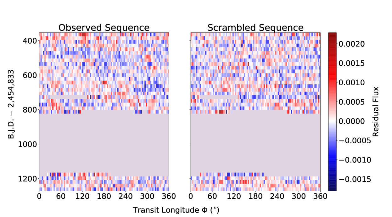
Figure 14.— Transit Tapestry of Kepler-423b Same as Figure 6 but for Kepler-423b. TCC analysis suggests a low stellar obliquity. Although there are hints of group-group correlation, we do not see prominent, long-lasting active regions. Similar to TrES-2, Kepler-423 may be faculae-dominated given its slow stellar rotation period (22 days). In contrast to the spot-dominated stars, Kepler-423 may not have persistent, localized features in the transit light curves.

4.10. WASP-85

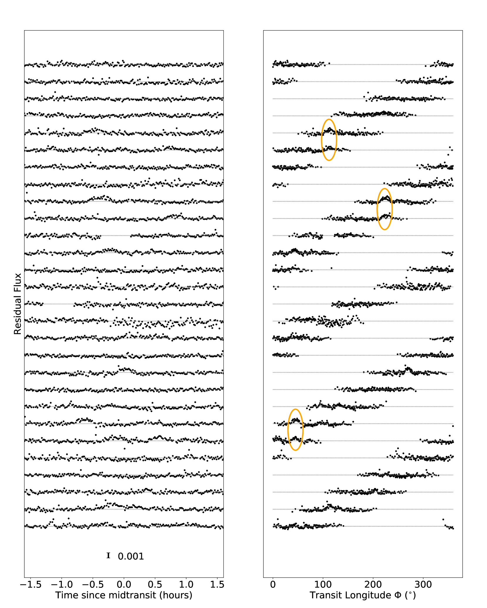
Figure 15.— K2 light curve of WASP-85 —Left: the residual flux (the observed transit light curve minus the best-fitting transit mode) as a function of time. —Right: the residual flux as a function of transit longitude $\Phi$ calculated with $P_{\text{tcc}}=15.2$ days. As shown with the orange ellipses, spot-crossing anomalies recur at fixed transit longitudes from one transit to the next unless the spot-crossing anomalies happen close to the ingress/egress of the transits. During the ingress/egress, geometrical foreshortening and limb darkening both weaken the signal of spot-crossing anomalies.

WASP-85Ab is a 2.7-day hot Jupiter around a G star in a visual binary system (Brown, 2015). The companion is a K star at an angular separation of about 1.5 arcseconds ($\sim$190 AU). Močnik et al. (2016a) analyzed the spot-crossing anomalies identified in the K2 short-cadence data for WASP-85A. They concluded that the recurrence of the spot-crossing events not only suggests a low stellar obliquity ($\lambda$ $\lesssim$ 14^∘), but also constrains the stellar rotation period to be $15.1\pm 0.6$ days. On the other hand, they measured the stellar rotation period to be $13.6\pm 1.6$ days based on the rotational modulation seen in the out-of-transit light curve.

We detect a TCC of $N_{\sigma}=4.5$ at $P_{\text{tcc}}=15.2\pm 0.3$ days. This is consistent with the value of $15.1\pm 0.6$ days reported by Močnik et al. (2016a). We measure a $P_{\text{phot}}$ = $13.28\pm 0.41$ days which was also consistent with the $13.6\pm 1.6$ days reported by Močnik et al. (2016a). Since the $N_{\sigma}$ of 4.5 is not as strong as the previous cases and the $P_{\text{tcc}}$ differ substantially from $P_{\text{phot}}$, we examined WASP-85 more closely.

The left panel of Figure 15 shows the residual flux of K2 short-cadence observation of WASP-85. After transforming time into transit longitude using $P_{\text{tcc}}=15.2$ days, the spot-crossing anomalies clearly recur at fixed transit longitude from one transit to the next, except in cases where spot-crossing events happened near the ingress or egress. Geometrical foreshortening and limb darkening effect are most severe during the ingress/egress; and both effects tend to weaken the signal of spot-crossing anomalies. Therefore the spot-crossing anomalies are expected to be suppressed here. The recurrence of spot-crossing events are compelling enough that we agree with Močnik et al. (2016a) that WASP-85Ab likely has a low stellar obliquity. The fact that $P_{\text{tcc}}=15.2\pm 0.3$ days disagrees with $P_{\text{phot}}$ = $13.28\pm 0.41$ days may be a sign differential rotation. Alternatively, this may be the result of the short lifetime of starspots. The rotational modulation in the K2 light curve underwent significant evolution during the $\approx$80 days of K2 observation suggesting a short spot lifetime. Furthermore, Figure 15 shows that many of crossed spots only persisted for days before disappearing.

The spot-crossing anomalies are about 0.0004-0.0008 in relative flux while the transit depth is about 2%. If the active regions uniformly fills the shadow of the planet, their relative intensity is hence 2-4% dimmer than the averaged photosphere. The spot-crossing events last about $\sim 15$ min or $\sim 20^{\circ}$ in longitude. After accounting for the blurring effect of the planet ($R_{p}/R_{\star}$ of 0.13), the spots are smaller than $5^{\circ}$. For WASP-85, we are likely seeing smaller, shorter-lived, individual starspots rather than the more stable and extended active regions on Kepler-17. Curiously, on the Sun, the lifetime of a sunspot is proportional to its size (Gnevyshev, 1938; Waldmeier, 1955). With this “GW rule” in mind, it is not surprising that the spots on WASP-85 have shorter lifetimes compared to the extended active regions on Kepler-17. We estimate the latitude probed by the transit chord as $3\pm 7^{\circ}$ using the the impact parameter of the transit of about 0.05 (Močnik et al., 2016a) and $R_{p}/R_{\star}$ of 0.13.

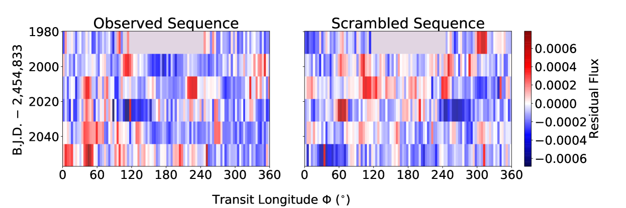
Figure 16.— Transit Tapestry of WASP-85b. Same as Figure 6 but for WASP-85. TCC of $N_{\sigma}$ = 4.5 is suggestive of a low obliquity. Close examination of Figure 15 showed that spot-crossing events did recur in neighboring transits. We agree with Močnik et al. (2016a) that WASP-85Ab likely has a low stellar obliquity. We are likely seeing the crossing of individual spots instead of extended active regions. This would explain the shorter lifetimes ($\sim 10$ days), weaker photometric signal and smaller size ($\sim 5^{\circ}$) of the anomalies seen in the transit light curves.

4.11. HAT-P-11

HAT-P-11b is a 4.9-day super-Neptune around a K dwarf. With a relatively large scaled orbital distance of $a/R_{\star}$ = 15.6, it is more akin to the “warm Jupiters” than hot Jupiters. Rossiter-McLaughlin observations revealed $\lambda=103^{+23}_{-10}$ degrees. Sanchis-Ojeda & Winn (2011) confirmed that the orbit is nearly perpendicular to the stellar equator by analyzing the spot-crossing anomalies seen in the Kepler light curve. They showed that spot-crossing anomalies cluster near two specific phases of the transit. They attributed this phenomenon to the presence of two active latitudes on the photosphere. As the planet transits the host star on a perpendicular orbit, the two symmetric active latitudes on both hemisphere will be occulted sequentially. The photometric signatures of the active regions are two persistent brightening features in the residual flux that remain fixed relative to the mid-transit time. Recent work by Morris et al. (2017a) mapped out the distribution of starspots on HAT-P-11 by explicitly modeling individual spot-crossing events. They drew attention to many similarities between sunspots and the starspots on HAT-P-11 such as size and latitudinal distribution. Morris et al. (2017b) showed that HAT-P-11 is chromospherically more active than other planet hosts with similar properties.

Béky et al. (2014a) reported that the ratio of spin period to orbital period is very nearly 6 to 1. Because of this commensurability, every six transits the planet and star return to the same configuration. As a result, the transiting planet can revisit the same active regions despite the high stellar obliquity. This results in a repeating pattern in the residual flux. Consequently, our TCC method detects a strong correlation ($N_{\sigma}$ = 6.0) even though the system is known to have a high obliquity. Visual inspection of the Kepler light curve shows that spot-crossing events only recur at fixed transit longitude after 6 consecutive transits. The close spin-orbit commensurability distinguishes HAT-P-11 from the low-obliquity systems discussed earlier.

4.12. Kepler-63

Kepler-63b is a sub-Saturn orbiting a G dwarf every 9.4 days. Sanchis-Ojeda et al. (2013) showed that the system has a high stellar obliquity ($\Psi$ = 104${}^{+22}_{-14}~{}^{\circ}$) using both Rossiter-McLaughlin observations and spot-crossing events in the Kepler light curve. Similar to HAT-P-11, Kepler-63 displays an apparent spin-orbit resonance (4:7 in this case). Similar to HAT-P-11, our TCC method finds a relatively strong signal ($N_{\sigma}$ = 5.8) even though the system has a high stellar obliquity. The strongest TCC is detected at $P_{\text{tcc}}$ = 37.7 $\pm$ 0.8 days (c.f. $P_{\text{phot}}$ = 5.041 $\pm$ 0.014 days) which coincide with the least common multiple between the stellar rotation period and the orbital period ($4P_{\text{orb}}$ or $7P_{\text{phot}}$) i.e. the period at which the system return to the same configuration. This is indicative of a spin-orbit commensurability rather than a low-obliquity orbit as we explained earlier.

4.13. Kepler-25

The two transiting planets b and c of Kepler-25, an F star, were confirmed by Steffen et al. (2012) via transit timing variations. Albrecht et al. (2013) performed Rossiter-McLaughlin measurement during the transits of planet c which is a sub-Saturn on a 12.7-day orbit. The Keck/HIRES data they obtained showed that Kepler-25c has a low stellar obliquity of $\lambda=-0.5\pm 5.7^{\circ}$. We applied the TCC method to the short-cadence Kepler light curve of Kepler-25. No statistically significant correlation was detected. The strongest TCC has $N_{\sigma}=3.2$ at $P_{\text{tcc}}=31\pm 1$ days. We could not measure the stellar rotation period independently in the out-of-transit light curve. Here and elsewhere in similar cases, we use the measured rotational broadening $v\rm{sin}i_{\star}$ and the stellar radius to estimate the stellar rotation period. For Kepler-25, Albrecht et al. (2013) reported $v\rm{sin}i_{\star}=9.5\pm 0.5$ km s^-1 and a stellar radius of $1.36\pm 0.13R_{\odot}$. Assuming an edge-on geometry ($i_{\star}$ = 90^∘), the stellar rotation period should be close to 7 days. The non-detection of correlation in the residual flux may be attributed to several possibilities. The SNR of any photometric signature of active regions is expected to be smaller since the transit depth is only about 0.1% (compared to the 1-4% for the strong TCC cases described earlier). The lack of rotational modulation in the out-of-transit light curve suggests that the host star ($T_{\text{eff}}\approx 6200\,K$) may not be magnetically active. Finally, the impact parameter of the planet is high ($b=0.881\pm 0.004$); the transit chord might have missed any active latitudes that are closer to the stellar equator.

4.14. CoRoT-11

CoRoT-11b is a 3.0-day hot Jupiter orbiting an F star, first reported by (Gandolfi et al., 2010). Later, Gandolfi et al. (2012) showed that the system has a low stellar obliquity ($\lambda=0.1\pm 2.6^{\circ}$) based on the Rossiter-McLaughlin effect. Our TCC analysis could not detect a statistically significant correlation ($N_{\sigma}=3.0$; $P_{\text{tcc}}=30\pm 4$ days; $P_{\text{phot}}$ unconstrained). Assuming an edge-on geometry ($i_{\star}=90^{\circ}$), the stellar rotation period should be close to 2 days ($v\rm{sin}i_{\star}=40\pm 5$ km s^-1 and $R_{\star}=1.37\pm 0.03R_{\odot}$, from Gandolfi et al., 2012). Similar to Kepler-25, the CoRoT-11 star may be too massive and hot ($T_{\text{eff}}\approx 6400\,K$) to be magnetically active. In addition the impact parameter is high ($b=0.8108\pm 0.0077$) and the transit chord might miss the active latitudes.

4.15. CoRoT-19

First reported by Guenther et al. (2012), CoRoT-19b is a hot Jupiter orbiting a F star every 3.9 days. Guenther et al. (2012) also measured the Rossiter-McLaughlin effect and found the sky-projected stellar obliquity to be $\lambda=-52^{+27}_{-22}~{}^{\circ}$. Our TCC analysis did not detect a statistically significant correlation ($N_{\sigma}=3.0$; $P_{\text{tcc}}=10\pm 1$ days; $P_{\text{phot}}$ unconstrained). The $v\rm{sin}i_{\star}$ argument gives a stellar rotation period close to 14 days ($v\rm{sin}i_{\star}=6\pm 1$ km s^-1 and $R_{\star}=1.65\pm 0.04R_{\odot}$, from Guenther et al., 2012). The non-detection of correlation is consistent with the high obliquity reported by Guenther et al. (2012). However, it might also be because the host star is too massive and hot ($T_{\text{eff}}\approx 6100\,K$) to be magnetically active.

4.16. WASP-47

WASP-47b is 4.2-day hot Jupiter around a G star (Hellier et al., 2012). Observations by K2 revealed two additional transiting planets in the system, thus making WASP-47b the first hot Jupiter known to have close-in planetary companions (Becker et al., 2015). Sanchis-Ojeda et al. (2015) measured the Rossiter-McLaughlin effect induced by the hot Jupiter WASP-47b, finding $\lambda=0\pm 24^{\circ}$.

We do not find a statistically significant correlation ($N_{\sigma}=3.0$; $P_{\text{tcc}}=6.3\pm 0.4$ days; $P_{\text{phot}}$ unconstrained). The stellar rotation period may be close to 37 days based on the combination of $v\rm{sin}i_{\star}=1.80^{+0.24}_{-0.16}$ km s^-1 and $R_{\star}=1.16\pm 0.26~{}R_{\odot}$ (Hellier et al., 2012; Sanchis-Ojeda et al., 2015). WASP-47 may be magnetically quiet, which is consistent with the lack of rotational modulation in the K2 light curve.

4.17. Kepler-13

Kepler-13Ab is 1.8-day hot Jupiter around an A star. Barnes et al. (2011) reported a misaligned orbit based on the asymmetric transit profile induced by gravity darkening. Later Doppler tomography (Johnson et al., 2014) and further analysis of gravity darkening (Masuda, 2015) showed that the system has a high obliquity ($\lambda=58.6\pm 2.0^{\circ}$).

Before applying our TCC method, we removed the best-fitting gravity darkening model (Masuda, 2015), rather than the usual transit model, in order to obtain the residual flux time series. No statistically significant correlation was detected. The strongest TCC has $N_{\sigma}=2.7$ at $P_{\text{tcc}}=3.12\pm 0.10$ days. However, Masuda (2015) reported a stellar rotation period close to one day. The lack of correlation is expected, given the high obliquity and the spectral type of the host star. Szabó et al. (2014) reported the detection of a 3:5 spin-orbit resonance based on a pattern seen in the residual flux. We did not detect a correlation at the stellar rotation period implied by the 3:5 spin-orbit resonance using the best-fitting gravity-darkened model from (Masuda, 2015).

4.18. CoRoT-3

CoRoT-3b is a 4.3-day brown dwarf ($21.66\pm 1.00~{}M_{\text{Jup}}$) transiting an F star (Deleuil et al., 2008). Triaud et al. (2009) performed Rossiter-McLaughlin observations which gave a constraint on the obliquity ($\lambda=37.6^{+10.0}_{-22.3}~{}^{\circ}$). We did not find a strong TCC; the maximum correlation has $N_{\sigma}=2.7$ and $P_{\text{tcc}}=24.3\pm 0.5$ days. The photometric rotation period is unconstrained. The $v\rm{sin}i_{\star}$ argument gives a stellar rotation period close to 3.0 days ($v\rm{sin}i_{\star}=17\pm 1$ km s^-1 and $R_{\star}=1.56\pm 0.09R_{\odot}$, from Deleuil et al., 2008). The non-detection of correlation is consistent with a mildly oblique orbit. Alternatively, it may be due to the magnetically inactive host star as indicated by the lack of rotational modulation in the CoRoT light curve.

4.19. CoRoT-18

CoRoT-18b is a 1.9-day hot Jupiter around a G star (Hébrard et al., 2011). Previous Rossiter-McLaughlin observations revealed a low stellar obliquity ($\lambda=-10\pm 20^{\circ}$). We find the strongest TCC of $N_{\sigma}=2.6$ at $P_{\text{tcc}}=15.7\pm 0.7$ days. On the other hand, the rotational modulation in the out-of-transit light curve suggests a rotation period of $P_{\text{phot}}=5.4\pm 0.4$ days. We cannot confirm the low stellar obliquity using our correlation method due to the lack of significant correlation and the disagreement between $P_{\text{tcc}}$ and $P_{\text{phot}}$. This may partly be attributed to the low SNR light curve of this 15th mag star.

4.20. Kepler-448

Kepler-448b is a 17.9-day warm Jupiter around a rapidly rotating F star ($v\rm{sin}i_{\star}=60.0\pm 0.9$ km s^-1 Bourrier et al., 2015). The Kepler light curve shows a 7.5-hour periodic modulation, presumably the stellar rotation period. The sky-projected obliquity has been determined through Doppler tomography to be $\lambda=12.6^{+3.0}_{-2.9}~{}^{\circ}$. We do not detect any statistically significant correlation ($N_{\sigma}=2.7$; $P_{\text{tcc}}=21.0\pm 0.6$ days; $P_{\text{tcc}}$ unconstrained). If the stellar rotation period is indeed 7.5 hours, the fast rotation has a similar timescale as the transit duration. Any photometric anomalies caused by active regions would likely be smeared out by the fast rotation.

4.21. Kepler-420

Kepler-420b is a 86.6-day warm Jupiter around a G dwarf. Santerne et al. (2014) used radial velocity data to show that the orbit has a high eccentricity of $0.772\pm 0.045$ and possibly a high stellar obliquity $\lambda=75^{+32}_{-46}~{}^{\circ}$. There is no strong TCC ($N_{\sigma}=2.5$; $P_{\text{tcc}}=11.7\pm 0.7$ days; $P_{\text{phot}}$ unconstrained). If the obliquity is low then the rotation period is close to 13.5 days, based on the reported values of $v\rm{sin}i_{\star}=4.6\pm 0.2$ km s^-1 and $R_{\star}=1.13\pm 0.14R_{\odot}$ (Santerne et al., 2014). The non-detection of correlations in the residual flux is consistent with an oblique orbit, although the host star may simply lack strong surface magnetic activity.

4.22. WASP-107

WASP-107b is a warm Jupiter ($a/R_{\star}=18.2$) around a K dwarf star (Anderson et al., 2017). Dai & Winn (2017) analyzed the short-cadence K2 light curve of WASP-107. They inferred that WASP-107 has a high stellar obliquity, with $\Psi=40-140^{\circ}$, because the observed spot-crossing anomalies did not recur in neighboring transits. The lack of recurrence also implied that the stellar rotation period and the planet’s orbital period cannot be in an exact spin-orbit resonance as previously suggested by Anderson et al. (2017). If the period ratio were exactly commensurate, spot-crossing anomalies would recur regardless of the stellar obliquity. The high obliquity of this system has now been confirmed by Rossiter-McLaughlin measurement which indicates a nearly perpendicular orbit (A. Triaud, private communication).

We applied the TCC method to the K2 light curve of WASP-107. The results show a weak signal, with $N_{\sigma}=2.5$ at $P_{\text{tcc}}=10.0\pm 0.5$ days. On the other hand, the rotational modulation in the out-of-transit light curve suggests a rotation period of $P_{\text{phot}}=17.1\pm 1.0$ days. The lack of significant correlation and the disagreement between $P_{\text{tcc}}$ and $P_{\text{phot}}$ are consistent with the oblique orbit.

4.23. Kepler-8

Kepler-8b is a 3.5-day hot Jupiter around an F star Jenkins et al. (2010). Albrecht et al. (2012) found $\lambda=5\pm 7^{\circ}$ based on observations of the Rossiter-McLaughlin effect. The strongest TCC analysis has $N_{\sigma}=2.2$ at $P_{\text{tcc}}=27.1\pm 0.3$ days. The rotational modulation in the out-of-transit light curve suggests a rotation period of $P_{\text{phot}}=28.64\pm 0.32$ days. The weak correlation in the residual flux may be attributed to the magnetically inactive host star ($T_{\text{eff}}$ = 6200 K). Moreover, the impact parameter of the planet is high $b=0.724\pm 0.020$.

4.24. HAT-P-7

HAT-P-7b is a hot Jupiter with an orbital period of 2.2 days and an F-type host star (Pál et al., 2008). Albrecht et al. (2012) observed the Rossiter-McLaughlin effect and found a high obliquity, with $\lambda=155\pm 37~{}^{\circ}$. Masuda (2015) measured the true obliquity, $\Psi=101\pm 2~{}^{\circ}$, based on the observable manifestations of gravity darkening effects in the Kepler transit light curves. As we did with Kepler-13, we removed the best-fitting gravity-darkening model to isolate any anomalies in the residual flux time series. No statistically significant TCC was detected. The strongest signal has $N_{\sigma}=2.0$ and $P_{\text{tcc}}=0.8\pm 0.2$ days, which conflicts with the rotation period of 1.5–2.1 days estimated by (Masuda, 2015).

4.25. WASP-75

WASP-75b is another hot Jupiter around an F star. The orbital period is 2.5 days. The system is distinguished by an unusually large transit impact parameter, $b=0.887\pm 0.008$. The K2 light curve reveals a stellar rotation period of $P_{\rm phot}=13.7\pm 1.1$ days. Gómez Maqueo Chew et al. (2013a) reported the projected rotation velocity ($v~{}sini_{\star}=4.3\pm 0.8$ km s^-1) and stellar radius ($1.26\pm 0.04~{}R_{\odot}$), leading to a weak constraint on the stellar inclination: $\sin i_{\star}>0.36$ with 95% confidence. We do not see a strong correlation in our TCC analysis. The strongest TCC has $N_{\sigma}=1.9$ at $P_{\text{tcc}}=22\pm 3$ days.

4.26. KIC 6307537

KIC 6307537 is an eclipsing binary system discovered with Kepler data. The star listed in the Kepler Eclipsing Binary Catalogue is a K dwarf. It eclipses the companion star every 29.7 days, causing the system brightness to fade by 7% for about 23 hours. When the companion occults the catalogued star, the system fades by 17%. This indicates that the companion is likely an evolved star, with a larger radius and lower effective temperature than the K dwarf. Prša et al. (2011) classified this system as an eclipsing binary of the Algol type (detached). The Kepler light curve also shows a clear rotational modulation of $78\pm 3$ days which we attribute to the slower rotation of the evolved star. From the separation between the primary and secondary eclipse, Van Eylen et al. (2016) obtained a constraint of the eccentricity: $e\cos\omega=0.0042\pm 0.0008$.

We apply the TCC method to the 7% eclipses of KIC 6307537, i.e., when the evolved star is being eclipsed. We detect a strong correlation ($N_{\sigma}=11.4$) in the residual flux at $P_{\text{tcc}}=80.4\pm 1.6$ days. This is consistent with the $P_{\text{phot}}=78\pm 3$ days. We interpret the strong TCC as evidence for a low obliquity of the evolved star. We place an upper bound of $\Psi\lesssim 6^{\circ}$. The agreement between $P_{\text{tcc}}$ and $P_{\text{phot}}$ not only supports the low-obliquity interpretation but also suggests that the rotational modulation in the out-of-eclipse light curve originates from the evolved star.

Figure 17 shows the eclipse tapestry. The tapestry suggests there are two active regions near longitudes of 40^∘ and 120^∘ each spanning about 5-10^∘ in longitude. The active regions appear wider in Figure 17 because of the finite radius ratio. With $R_{1}/R_{2}\approx 0.24$, the photometric features due to the active regions are broadened by about 30^∘ in longitude. These photometric features in the residual flux had amplitudes of about 1-2% in relative flux. Comparing with the eclipse depth of about 7%, the active regions on average were roughly 15-30% dimmer than the photosphere. The active regions seem to have lasted the entire Kepler campaign indicating a lifetime of at least $10^{3}$ days.

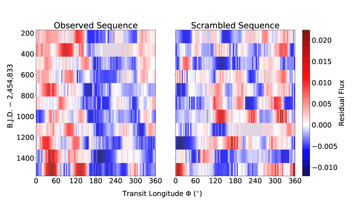
Figure 17.— Eclipse Tapestry of KIC 6307537. Same as Figure 6 but for the eclipsing binary system KIC 6307537. We find a strong TCC consistent with a low stellar obliquity for the larger star in the system. There are two active regions near transit longitudes of 40^∘ and 120^∘. The lifetime of these active regions are at least $10^{3}$ days, longer than those inferrred for the dwarf stars described earlier.

4.27. KIC 5193386

KIC 5193386 is another Kepler eclipsing binary system. One set of eclipses occurs every 21.4 days, during which the total light decreases by 8% for about 22 hours. The other set of eclipses is deeper (24%) and flat-bottomed. The secondary star (the star being eclipsed during the 8% fading events) is likely evolved, with a larger radius and lower effective temperature than its companion. We measure a rotational modulation of $26.0\pm 0.8$ days in the Kepler light curve. From the separation between the primary and secondary eclipse, Van Eylen et al. (2016) constrained the eccentricity: $e\cos\omega=-0.0022\pm 0.0015$.

By analyzing the 8% eclipses we find a strong TCC, with $N_{\sigma}=9.5$ and $P_{\text{tcc}}=25.8\pm 0.3$ days, indicating a low obliquity ($\Psi\lesssim 14^{\circ}$). Figure 18 shows the tapestry. During the early stages of Kepler observations, one prominent active region was located at a transit longitude of 30^∘. It gradually split into two distinct active regions that separated longitudinally from each other. Again, we interpret this phenomenon as the emergence of a magnetic flux tube and the subsequent separation of the two footprints of the tube on the stellar photosphere. The active regions are consistent of being about 10^∘ wide and are 10–25% fainter than the photosphere.

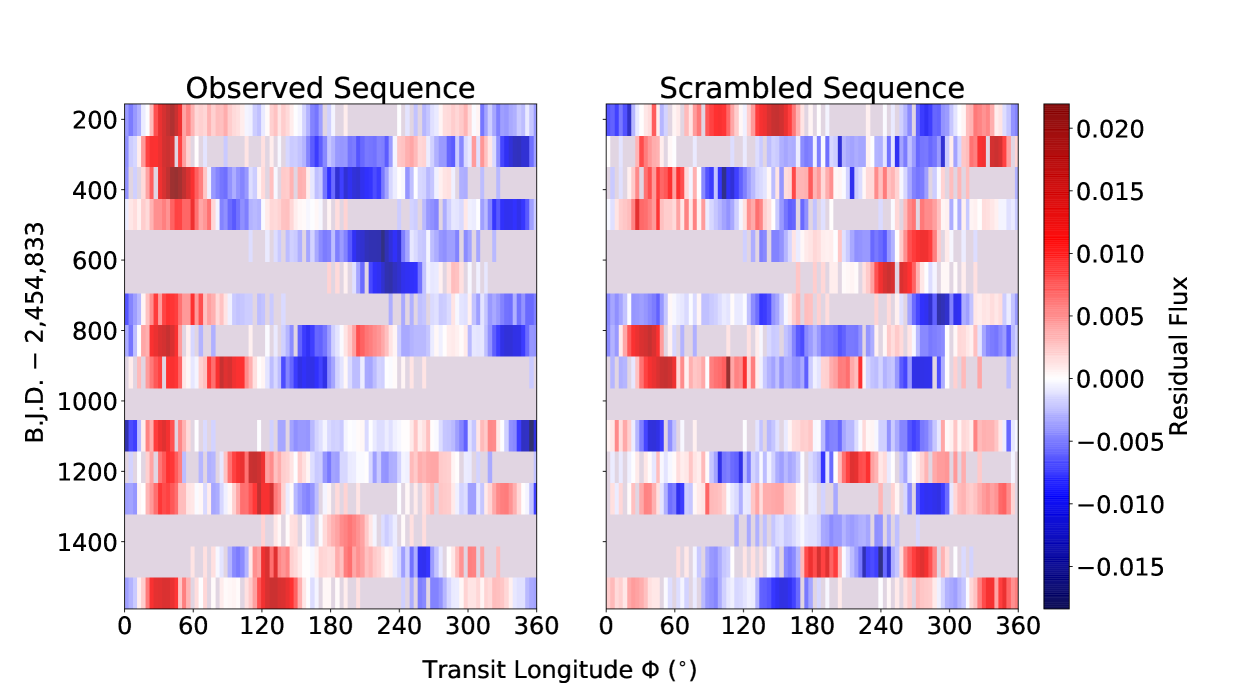
Figure 18.— Eclipse Tapestry of KIC 5193386. Same as Figure 6 but for the eclipsing binary system KIC 5193386. The strong TCC detected suggests a low obliquity for the larger, likely evolved star of the system. One prominent active region was located at transit longitude $30^{\circ}$ at the start of the Kepler observation. It then split into two distinct regions that separated longitudinally from each other. This may be the result of an emerging magnetic flux tube.

4.28. KIC 6603756

KIC 6603756 is an eclipsing binary system in the Kepler catalog of Prša et al. (2011), who classified this system as an eclipsing binary of the Algol type (detached). Only one set of eclipses was detected. These 4% eclipses last for about 6 hours and repeat every 5.2 days. The Kepler light curve shows a clear rotational modulation of 6.128 $\pm$ 0.054 days.

Our TCC analysis gives a strong correlation, $N_{\sigma}=9.2$, at $P_{\text{tcc}}=6.0\pm 0.1$ days. We interpret the strong TCC as a sign of a low obliquity for eclipsed star and place an upper bound of $\Psi\lesssim 12^{\circ}$. Figure 19 shows the eclipse tapestry. Active regions seemed to occur preferentially near a transit longitude of 230^∘ throughout the 300 days of Kepler observations. These photometric features in the residual flux had amplitudes of about 0.002–0.006 in relative flux which, when compared to the eclipse depth of 4%, implies that the implying that the active regions were on average 5–15% dimmer than the photosphere.

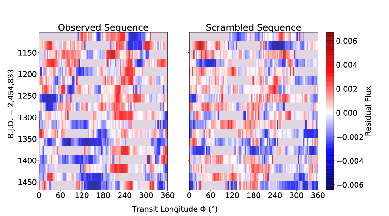
Figure 19.— Eclipse Tapestry of KIC 6603756. Same as Figure 6 but for the eclipsing binary system KIC 6603756. TCC analysis revealed a low-obliquity for this system. Active regions seem to occur preferentially near transit longitude of 230^∘ throughout the 300 days of Kepler observations.

4.29. KIC 5098444

KIC 5098444 is a Kepler eclipsing binary with 2% primary eclipses and 0.4% secondary eclipses (occultations), and an orbital period of 26.9 days. The Kepler light curve shows a clear rotational modulation of 23.49 $\pm$ 0.19 days. The primary eclipses, analyzed here, have a duration of about 11 hours. The TCC is strong, with $N_{\sigma}=7.9$ and $P_{\text{tcc}}=23.40\pm 0.24$ days. We conclude the primary star has a low obliquity, with $\Psi\lesssim 8^{\circ}$. The agreement between $P_{\text{tcc}}$ and $P_{\text{phot}}$ also shows that the rotational modulation in the out-of-eclipse light curve originates from the primary.

Figure 20 is the eclipse tapestry. An active region near transit longitude of 90^∘ persisted throughout the 800 days of Kepler observations. The flux anomalies have amplitudes of 0.5–1%. Comparing with the eclipse depth of about 2%, the active regions on average were roughly 20-50% dimmer than the photosphere. The active regions span about 40^∘ in longitude after accounting for the finite size of the secondary.

Figure 20.— Eclipse Tapestry of KIC 5098444. Same as Figure 3, but for the eclipsing binary system KIC 5098444. TCC analysis suggests a low stellar obliquity for the primary. An active region (40^∘ wide, 20-50% dimmer than average photosphere) near transit longitude of 90^∘ persisted throughout the 800 days of Kepler observations.

4.30. KIC 7767559

KIC 7767559 was originally listed as a planetary candidate, KOI-895. This system was later classified as an eclipsing binary due to the detection of significant secondary eclipses. The primary eclipse occurs every 4.4 days with a depth of 1% and a duration of 3.9 hours. The Kepler light curve shows a clear rotational modulation of $P_{\text{phot}}$ = 5.02 $\pm$ 0.20 days. Holczer et al. (2015) detected a strong correlation between TTV and local flux variation, indicating a prograde orbit.

The 1% primary eclipses show a strong TCC with $N_{\sigma}=7.7$ at $P_{\text{tcc}}=5.1\pm 0.1$ days. We place an upper bound on the obliquity, $\Psi\lesssim 7^{\circ}$. Figure 21 shows the Eclipse Tapestry. Although there are signs of group-group correlation, any large-scale, long-lasting active regions are not visually obvious.

Figure 21.— Eclipse Tapestry of KIC 7767559. Same as Figure 6 but for the eclipsing binary system KIC 7767559. A strong TCC signal indicates a low obliquity for the primary star.

4.31. KIC 5376836, 3128793, 5282049, 5282049

KIC 5376836, 3128793, 5282049, 5282049 are all eclipsing binary systems discovered by Kepler. In all cases our analysis revealed strong TCC signals, with $N_{\sigma}$ = 5–7, and TCC periods that agree with the independently measured photometric periods. We put an upper bounds on the obliquity $\Psi\lesssim$ 3 to 20^∘ (See Table LABEL:tab:eb). Figure 22 shows the eclipse tapestries for each system, all of which lack high-contrast, long-lasting active regions.

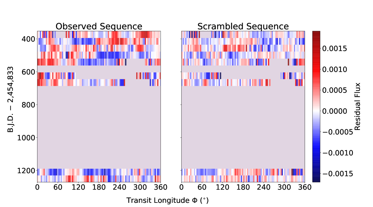
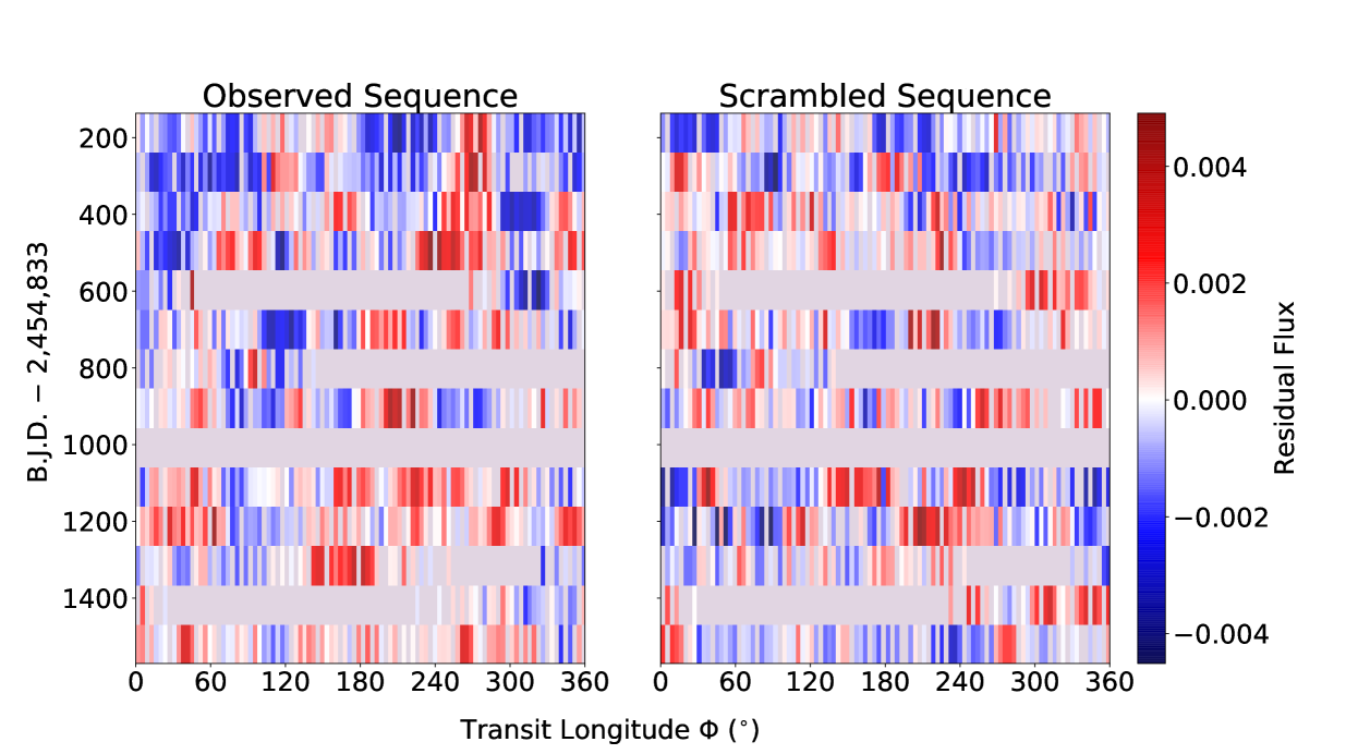
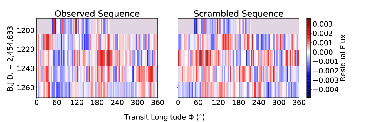
Figure 22.— Eclipse Tapestry of KIC 5376836, 3128793, 5282049, 5282049. Same as Figure 6 but for these four eclipsing binary system from top to bottom. The strong TCC and the agreement between $P_{\text{tcc}}$ and $P_{\text{phot}}$ suggest low stellar obliquity for all four systems. However, the correlations are not obvious to the eye.

5. Discussion and Conclusion

5.1. The TCC method

As any other method to obtain information on stellar obliquities, the TCC method has strengths and weaknesses. One of the advantages of the TCC method is that it does not make any assumption about the size, shape and intensity distribution of the active regions. In contrast, the traditional spot-tracking methods (e.g. Sanchis-Ojeda et al., 2011; Tregloan-Reed et al., 2013; Béky et al., 2014b) often assume circular and uniform starspots for ease of modeling. The TCC method looks for recurrence in the residual flux regardless of the shape of the recurring pattern. Therefore it can handle spots of arbitrary shape and intensity distribution and even bright active regions such as plages and faculae.

We have created transit tapestries to allow the properties of the active regions on transit chord to be tracked and visualized in a model-independent manner. The TCC statistic combines all the data together, and can therefore be effective even in systems with lower SNR for which no features can be discerned in the transit tapestry. In contrast, the traditional spot-tracking method is based on the visual identification of individual spot-crossing events. This is more subjective and is only possible in the systems for which the data have the highest SNR. The TCC method is largely automated and does not require additional follow-up observations, facilitating the application to a large sample of systems.

One of the limitations of the TCC method is that it requires light curves with a high temporal sampling rate. This is because the durations of spot-crossing events are similar to the brief durations of the ingress and egress phases of the transit. Continuous monitoring of the system is also very important for the TCC method. Continuous monitoring enables an independent check on the stellar rotation period $P_{\text{phot}}$ from the rotational modulation in the out-of-transit light curve. Moreover, active regions have a limited lifetime, and may drift in longitude and latitude. The recurring pattern in residual flux caused by active regions may quickly change or disappear after a few transits. This is why it is important to observe many pairs of neighboring transits, separated by a relatively short amount of time.

In the TCC method, the detection of a strong correlation requires a confluence of factors. The host star must be magnetically active, with stable active regions. Unless the system is close to a spin-orbit commensurability, the stellar obliquity $\Psi$ must be nearly 0^∘ or 180^∘, such that the planet repeatedly transits the same active regions. In addition, the impact parameter of a transiting planet must be such that the transit chord overlaps with the active latitudes on the host star. On the other hand, when no strong TCC is observed, the system is not guaranteed to have a high obliquity, as the failure of any of the preceding conditions could explain the lack of correlation. Therefore the TCC method is best at picking out stars with obliquities that are very low or are close to exactly retrograde. In contrast, the Rossiter-McLaughlin effect can lead to tight constraints for just about any angle, although it is only sensitive to the sky-projected obliquity $\lambda$.

5.2. Detected low-obliquity systems

We applied the TCC method to selected CoRoT, Kepler and K2 transiting planets and planetary candidates. We found 10 cases in which the star has a low obliquity (see Table 1). Among these, five were not previously known to have a low obliquity: Kepler-71b, KOI-883.01, Kepler-45b, Kepler-762b and Kepler-423b. For the other five systems, we confirmed the low stellar obliquities reported previously. Notably, all of these low-obliquity detections are for stars with giant planets ($R_{p}>0.9~{}R_{\text{Jup}}$), with scaled semi-major axis $a/R_{\star}<12$. This is not too surprising; the requirements for a relatively high SNR and many consecutive transits are most easily met for close-in giant planets.

All of these low-obliquity stars are G and K dwarfs, with the sole exception of Kepler-45, which is an M dwarf. The low obliquities of the G and K dwarfs are consistent with the general trend that hot Jupiters around relatively low-mass stars below the Kraft break tend to have low obliquities (Winn et al., 2010a). The presence of a convective outer layer in these low-mass stars may be also crucial for the generation of stellar magnetic activity. In contrast, several previously reported low-obliquity systems (Kepler-25c, CoRoT-11b and Kepler-8b) with more massive host stars did not show strong TCC. This may be ascribed to the lack of magnetic activity; these stars have effective temperatures exceeding the Kraft break, and do not have thick outer convective zones.

Kepler-45 is only the second M dwarf for which the stellar obliquity has been measured, the other one being GJ 436 (Bourrier et al., 2017). As noted in the introduction, the distribution of stellar obliquities has been observed to depend on the properties of the host star. Winn et al. (2010a) found that the stars above and below the Kraft (1967) break have different obliquity distributions. Stars cooler than about 6250 K have thick convective envelopes, while hotter stars have radiative envelopes. The differing obliquity distributions may be related to the differing magnetic fields, tidal dissipation rates, or rotational histories of the stars on either side of this boundary. Performing obliquity measurements on a wider range of stellar types may help to clarify the situation. This is especially true for M dwarfs which may be completely convective and for which obliquity measurements have been very limited. Rossiter-McLaughlin observations have not been very successful for M dwarfs, because of their higher stellar variability, slower stellar rotation, and faint optical magnitudes, all of which hinder the acquisition and interpretation of high-resolution spectra. The TCC method may be particularly useful for M dwarfs because high levels of activity and slow rotation are actually favorable for the technique, and because high-resolution spectroscopy is not needed.

As we mentioned previously, the TCC method is capable of identifying both well-aligned and perfectly retrograde systems. However, among the 64 planetary systems and 24 eclipsing binaries in our sample, none were found with a strong TCC corresponding to a retrograde orbit. In particular, all 10 of the planetary systems that had a strong TCC were found to have very well-aligned orbits, even though retrograde orbits would have been equally easy to detect. All 10 of the systems feature cool stars, below the Kraft break. Thus the results for these 10 systems is further evidence that cool stars with hot Jupiters mainly have prograde orbits rather than retrograde orbits.

5.3. Constraints on stellar magnetic activity

The properties of sunspots have been tracked since the 18th century. It is well known that sunspots preferentially emerge at latitudes of about $30^{\circ}$ north or south of the equator at the start of a magnetic cycle (Hathaway, 2015). These active latitudes gradually drift towards the equator as the magnetic cycle continues, giving rise to the “butterfly diagram” when spot latitudes are plotted against time. It has also been noted that sunspots tend to cluster at certain active longitudes (see e.g. Bumba & Howard, 1965). Other solar magnetic phenomena such as flares, coronal mass ejections, and X-ray emission are also associated with active longitudes (Zhang et al., 2008; Gyenge et al., 2017; Zhang et al., 2007). Typically there are two active longitudes on the Sun separated by 180^∘, each of which has a width of order 20^∘ (Berdyugina & Usoskin, 2003). At solar maximum there can be as many as four active longitudes, and at solar minimum active longitudes may disappear (de Toma et al., 2000). The lifetime of active longitudes has been found to be seven rotation cycles (de Toma et al., 2000) and perhaps even as long as a century (Berdyugina & Usoskin, 2003). While the exact physical mechanism responsible for persistently active longitudes is still unknown, they do not seem to be a unique property of our Sun. Lanza et al. (2009) and García-Alvarez et al. (2011) found evidence for active longitudes on other stars too.

The transit tapestries of several low-obliquity systems with high SNR and strong magnetic activity — Kepler-17b, CoRoT-2b, Qatar-2b, Kepler-71b and KOI-883.01 — allow us to track the size, contrast, lifetime and latitudinal distribution of the active regions along the transit chords of these planet-hosting stars. These are the most magnetically active among the systems we have studied. We summarize the properties of the active regions of these systems in Table 3.

We note the following trends. In all cases the Rossby number — the ratio between the rotation period and the convective overturn time — is smaller than that of the Sun. The Rossby number is routinely used for expressing thresholds and scaling relations in the study of stellar magnetic activity and magnetic braking (see, e.g., van Saders et al., 2016). The strong magnetic activity that is characteristic of our sample is linked to their fast rotation. All five stars are below the Kraft break. The typical contrast of the active regions is on the order of 10% in the wide optical bandpasses of the Kepler and CoRoT data. The typical lifetime of the active regions is on the order of 100 days, although we note that the inferred lifetime of the active longitudes is degenerate with the rate of latitudinal migration. If the active regions migrate away from the transit chord, the active regions will no longer cause photometric signatures in the transit light curve.

For all of the systems in Table 3, there are typically two active longitudes that are present on the same stellar latitude simultaneously. At a given time there may be no active longitudes or as many as four, similar to the Sun. Interestingly, the size, contrast, and the lifetime of the different active regions on the same stars are very similar to each other. The latitude probed by the planet is $\lesssim$20^∘ in all cases, suggesting that active regions tend to occur at these low latitudes, which is also similar to the situation on the Sun. If active regions had no preferred latitudes, the systems in Table 3 might have shown a broader distribution of transit impact parameters.

Montet et al. (2017) noted a pattern in the origin of photometric variability of Sun-like stars observed by Kepler ($T_{\rm eff}$ within 150 K of the solar value and $\log g>4.2$). The brightness variations of stars with rotation periods shorter then 25 days are consistent with those produced by dark spots, while slower rotators are more consistent with bright spots (plages and faculae). The most magnetically active systems in our sample (Table 3) are all consistent with being spot-dominated. This is inferred from the prevalence of positive residuals seen in the transit tapestries. For the slower rotators in our sample, TrES-2 and Kepler-423, we did not observe strong features in the transit tapestries, perhaps because the active regions are faculae spanning a larger angular size.

5.4. Eclipsing binaries

We now turn to the eclipsing binaries in our sample. We found eight Kepler eclipsing binaries that show strong correlation and good agreement between $P_{\text{phot}}$ and $P_{\text{tcc}}$ (see Table LABEL:tab:eb). It is more difficult to detect and interpret the TCC signals for these systems. Due to the lack of follow-up observations, little is known about the properties of the stars in these binaries. The stellar parameters in Table LABEL:tab:eb were estimated from fitting stellar models and evolutionary tracks to archival broadband photometry (Prša et al., 2011). Moreover, only the properties of the primary stars were reported. Second, because of the larger radius ratio in these binaries, the TCC method provides poor angular resolution for probing the active regions. Furthermore, some of the eclipsing binaries were only observed in the long-cadence mode. The 30-minute time averaging smears out the photometric patterns of active regions. Finally the orbital periods of some binaries are longer than 20 days. This means we have a smaller number of eclipses to analyze, and leaves the active regions more time in between eclipses for their properties to change, weakening the TCC signal.

Nonetheless, we do see good evidence of active regions in the eclipse tapestries of KIC 6307537, KIC 5193386 and KIC 5098444. Given the shallow eclipse depths and long eclipse durations, one of the stars in each of these binaries is likely evolved. This is further supported by the deeper and flat-bottomed eclipse seen in KIC 6307537 and KIC 5193386 which indicates the eclipsed star has a larger radius and lower effective temperature than the eclipsing star. The active regions extend by about $10^{\circ}$ in longitude and are on the order of 10% fainter than the rest of the photosphere. We did not detect significant longitudinal migration except for KIC 5193386, where one active region gradually split into two regions that drifted apart in longitude. These regions may be the two footprints of an emerging magnetic flux tube. The active regions on these evolved stars persisted for longer than those on the planet-hosting dwarf stars, up to at least a thousand days.

The low obliquities of these binaries could be a consequence of tidal evolution, which tends to bring stars into a double-synchronous aligned configuration. However we note that the all eight of the low-obliquity binary systems have not achieved a state of synchronized rotation: $P_{\rm{orb}}\neq P_{\rm{rot}}$ (see Table LABEL:tab:eb). Thus the low-obliquity state may reflect the initial conditions of formation, rather than the outcome of tidal evolution.

5.5. Future prospects

Crucial to the success of the TCC methods are light curves with high SNR, high cadence, and continuous time coverage for many orbital and rotation periods. New opportunities for applying TCC will be provided by the existing and upcoming space-based missions TESS (Ricker et al., 2014), CHEOPS (Broeg et al., 2013), and PLATO. The TESS mission, scheduled for launch in 2018, will provide a fresh sample of transiting planets which will be suitable targets for the TCC analysis. The plan for the mission is to obtain data with 2-minute cadence for several hundred thousand preselected target stars. This will be ideal for resolving the photometric signatures of active regions. Most TESS stars will only be observed for one month during the two-year primary mission, but a small fraction of the stars (near the ecliptic poles) will be observed for as long as a year. Our best hopes are for TESS targets that are observed for at least a few months, similar in duration to the 80-day K2 campaigns that have already yielded some strong detections with the TCC method. Using the TESS mission simulations of Sullivan et al. (2015) and Bouma et al. (2017), we have made a rough estimate that there will be a few dozen TESS planets with single-transit SNR $>50$, amenable to TCC analysis.

Table 1List of Planetary Systems of Searched

	Status	$P_{\text{orb}}$ (days)	$a/R_{\star}$	$M_{p}$ ($M_{\text{Jup}}$)	$R_{p}$ ($R_{\text{Jup}}$)	$M_{\star}$ ($M_{\odot}$)	$R_{\star}$ ($R_{\odot}$)	$T_{\text{eff}}$ (K)	$P_{\text{phot}}$ (days)	$P_{\text{tcc}}$ (days)	$N_{\sigma}$	$P_{\text{tcc}}$/$P_{\text{orb}}$	$\Psi_{\text{Upper}}$ (∘)	$\lambda_{\text{lit}}$(∘)	Ref.
Kepler-17b	Confirmed	1.4857108(2)	5.48(2)	2.450(14)	1.312(18)	1.16(6)	1.05(3)	5781(85)	11.9$\pm$1.1	11.8(7)	59.6	7.94	¡10	¡ 15	Désert et al. (2011)
CoRoT-2b	Confirmed	1.7429964(17)	6.70(3)	3.31(16)	1.465(29)	0.97(6)	0.902(18)	5575(66)	4.530(68)	4.5(3)	22.6	2.58	¡4	4.7$\pm$12.3	Alonso et al. (2008); Nutzman et al. (2011)
Qatar-2b	Confirmed	1.3371182 (37)	6.52(10)	2.487(86)	1.144(35)	0.740(37)	0.713(18)	4645(50)	18.5 $\pm$1.9	18.2(4)	18.0	13.61	¡11	0$\pm$10	Esposito et al. (2017)
Kepler-71b	Confirmed	3.905081(72)	11.92(15)		1.11(2)	0.95(5)	0.86(2)	5591(105)	19.87(18)	19.7(8)	10.7	5.04	¡6	Prograde	Howell et al. (2010); Holczer et al. (2015)
KOI-883.01	Candidate	2.688899317(109)	10.40		1.05(13)	0.702(63)	0.643(81)	4809(151)	9.11(11)	9.1(2)	9.2	3.38	¡4	Prograde	ExoFOP; Holczer et al. (2015)
Kepler-45b	Confirmed	2.455239(5)	10.6 $\pm$ 1.0	0.51(9)	0.96(11)	0.59(6)	0.55(11)	3820(90)	15.8(2)	16.7(8)	6.3	6.80	¡11		Johnson et al. (2012)
TrES-2b	Confirmed	2.4706133738(187)	7.98(17)	1.253(52)	1.189(25)	0.98(62)	1.000(36)	5850(50)	28.35(34)	29.9$\pm$1.4	5.8	12.10	¡10	9$\pm$12	Winn et al. (2008)
Kepler-762b	Confirmed	3.7705521(94)	8.16		1.10(56)	1.06(7)	1.08(23)	5944(124)	4.045(25)	4.0(1)	5.2	1.06	¡16	Prograde	ExoFOP; Holczer et al. (2015)
Kepler-423b	Confirmed	2.68432850(7)	8.106${}^{+0.117}_{-0.259}$	0.595(81)	1.192(52)	0.85(4)	0.95(4)	5560(80)	22.047(121)	23.0(9)	4.7	8.57	¡10		Gandolfi et al. (2015)
WASP-85b	Confirmed	2.6556777(44)	8.79(23)	1.265(65)	1.24(3)	1.04(7)	0.96(13)	5685(65)	13.28(41)	15.2(3)	4.5	5.69	¡7	¡ 14	Močnik et al. (2016a)
HAT-P-11b	Confirmed	4.887802443(30)	15.58${}^{+0.17}_{-0.82}$	0.08243(90)	0.42(13)	0.81(3)	0.75(2)	4780(50)	29.472(134)	29.34(30)	6.0	6.00		$103^{+26}_{-10}$	Winn et al. (2010c)
Kepler-63b	Confirmed	9.4341505(10)	19.12(8)	¡120	0.545(20)	0.984(40)	0.901(27)	5576(50)	5.401(14)	37.7(8)	5.8	4.00		$-110^{+22}_{-14}$	Sanchis-Ojeda et al. (2013)
CoRoT-16b	Confirmed	5.35227(20)	11.20${}^{+1.21}_{-1.09}$	0.535(85)	1.17(14)	1.098(78)	1.19(14)	5650(100)		4.0(4)	3.9	0.75			Ollivier et al. (2012)
WASP-55b	Confirmed	4.465633(4)	10.81(14)	0.57(4)	1.30(5)	1.013(37)	1.011(36)	5900(100)		27(2)	3.5	6.05			Hellier et al. (2012)
CoRoT-17b	Confirmed	3.7681(3)	6.23(24)	2.43(30)	1.02(7)	1.04(1)	1.59(7)	5740(80)		17(2)	3.5	4.51			Csizmadia et al. (2011)
CoRoT-22b	Confirmed	9.75598(11)	17.30${}^{+1.3}_{-0.57}$	12.2${}^{+14}_{-8.8}$	0.435${}_{-0.035}^{+0.015}$	1.099(49)	1.136(90)	5939(120)		25(2)	3.2	2.56			Moutou et al. (2014)
CoRoT-24b	Confirmed	5.1134(6)	10.9 $\pm$ 2.8	¡0.018	0.33(4)	0.91(9)	0.86(9)	4950(150)		14(1)	3.2	2.74			Alonso et al. (2014)
Kepler-25c	Confirmed	12.7203678(35)	18.52(24)	0.045(8)	0.4598(54)	1.22(6)	1.36(13)	6190(80)	23.21(27)	29.2(7)	3.2	2.30		0.5$\pm$5.7	Albrecht et al. (2013)
CoRoT-13b	Confirmed	4.03519(3)	10.81(32)	1.308(66)	0.885(14)	1.09(2)	1.01(3)	5945(90)		20.6(6)	3.1	5.11			Cabrera et al. (2010)
CoRoT-11b${}^{\rm\ref{note1}}$	Confirmed	2.994330(11)	6.890(80)	2.33(34)	1.430(33)	1.27(5)	1.36(13)	6440(120)		30(4)	3.0	10.02		0.1$\pm$2.6	Gandolfi et al. (2012)
CoRoT-19b	Confirmed	3.89713(2)	6.7(1)	1.11(6)	1.29(5)	1.21(6)	1.65(4)	6090(70)		10(1)	3.0	2.57		-52${}^{+27}_{-22}$	Guenther et al. (2012)
WASP-47b${}^{\rm\ref{note1}}$	Confirmed	4.1591287(49)	9.715(50)	1.123(510)	1.17(79)	1.11(49)	1.16(26)	5576(67)		6.3(4)	3.0	1.51		0$\pm$24	Sanchis-Ojeda et al. (2015)
CoRoT-14b	Confirmed	1.51214(13)	4.78(28)	7.6(6)	1.09(7)	1.13(9)	1.21(8)	6035(100)		5.4(8)	2.9	3.57			Tingley et al. (2011)
CoRoT-8b	Confirmed	6.21229(3)	17.6(4)	0.22(3)	0.569(20)	0.88(4)	0.77(2)	5080(80)		25.3(0.3)	2.8	4.07			Bordé et al. (2010)
CoRoT-25b	Confirmed	4.86069(6)	10.2${}^{+1.1}_{-0.5}$	0.27(4)	1.08 ${}_{-0.1}^{+0.3}$	1.09${}_{-0.05}^{+0.11}$	1.19 ${}_{-0.03}^{+0.14}$	6040(90)		31(1)	2.8	6.38			Almenara et al. (2013)
KOI-212.01	Candidate	5.6959023(15)	12.2		0.58(23)	1.013(135)	0.94(38)	6106(156)	16.295(336)	33(1)	2.8	5.79			ExoFOP
CoRoT-6b	Confirmed	8.886593(4)	17.94(33)	2.96(34)	1.166(35)	1.055(55)	1.025(26)	6006(73)	6.35(13)	5.4(2)	2.8	0.61			Fridlund et al. (2010)
Kepler-13Ab	Confirmed	1.7633587(20)	3.16(8)	6.6$\pm$1.5	1.335${}_{-0.264}^{+0.484}$	1.49${}_{-0.18}^{+0.22}$	1.80${}_{-0.36}^{+0.65}$	8500(400)		3.12(10)	2.7	1.77		58.6$\pm$2.0	Masuda (2015)
CoRoT-3b	Brown Dwarf	4.256800(5)	7.8(4)	21.7 $\pm$ 1.0	1.01(7)	1.41(8)	1.44(8)	6740(140)		24.3(5)	2.7	5.71		-37.6${}^{+22.3}_{-10.0}$	Deleuil et al. (2008); Triaud et al. (2009)
HATS-9b	Confirmed	1.9153073(52)	4.36${}^{+0.10}_{-0.25}$	0.837(29)	1.40(6)	1.28(13)	1.32(7)	5366(70)		13.6$\pm$1.1	2.7	7.10			Brahm et al. (2015)
Kepler-471b	Confirmed	5.01423457(59)	8.3		0.94(69)	1.314(257)	1.271(927)	6475(169)	26.51(57)	20.5(8)	2.7	4.09			ExoFOP
Kepler-494b	Confirmed	8.0251182(23)	11.5		0.637(118)	1.10(7)	1.26(23)	5513(184)	8.985(186)	30.1(4)	2.6	3.75			ExoFOP
CoRoT-12b	Confirmed	2.828042(13)	7.74(18)	0.917(70)	1.44(13)	1.078(72)	1.116(92)	5675(80)		9.8(8)	2.6	3.47			Gillon et al. (2010b)
CoRoT-18b${}^{\rm\ref{note1}}$	Confirmed	1.9000693(28)	6.35(40)	3.47(38)	1.31(18)	0.95(15)	1.00(13)	5440(100)	5.4(4)	15.7(7)	2.6	8.26		-10$\pm$20	Hébrard et al. (2011)
CoRoT-28b	Confirmed	5.20851(38)	7.29(16)	0.484(87)	0.955(66)	1.01(14)	1.78(11)	5150(100)		41(3)	2.6	7.87			Cabrera et al. (2015)
Kepler-448b${}^{\rm\ref{note1}}$	Confirmed	17.8552333(9)	18.8(4)	¡ 10	1.43(13)	1.452(93)	1.63(15)	6820(120)	1.245(124)	21.0(6)	2.6	1.18		12.6${}^{+3.0}_{-2.9}$	Bourrier et al. (2015)
CoRoT-21b	Confirmed	2.72474(14)	4.60(26)	2.26(31)	1.30(14)	1.29(9)	1.95(21)	6200(100)		16.7(5)	2.5	6.13			Pätzold et al. (2012)
Kepler-420b	Confirmed	86.647661(34)	155.4$\pm$2.4	1.45(35)	0.94(12)	0.99(5)	1.13(14)	5520(80)		11.7(7)	2.5	0.14		75${}^{+32}_{-46}$	Santerne et al. (2014)
Kepler-74b	Confirmed	7.340718(1)	11.8${}^{+1.4}_{-0.8}$	0.68(9)	1.32(14)	1.4${}_{-0.11}^{+0.14}$	1.51(14)	6050(110)	26.7(8)	36$\pm$1.2	2.4	4.90			Hébrard et al. (2013)
Kepler-96b	Confirmed	16.2385	21.2	0.027(11)	0.238(20)	1.00(6)	1.02(9)	5690(73)	14.922(83)	42.7$\pm$1.7	2.3	2.63			Marcy et al. (2014)
Kepler-485b	Confirmed	3.2432598(18)	8.2		1.286${}^{+0.302}_{-0.145}$	1.07(8)	1.09(26)	5958(153)	30.72(45)	22.8$\pm$1.1	2.3	7.03			ExoFOP
CoRoT-7b	Confirmed	0.85353(2)	4.27(20)	0.0149(30)	0.149(8)	0.93(3)	0.87(4)	5275(75)	22.4$\pm$3.6	2.5(2)	2.3	2.93			Léger et al. (2009)
CoRoT-29b	Confirmed	2.850570(6)	9.22(19)	0.85(20)	0.90(16)	0.98(14)	0.90(12)	5260(100)		16.1$\pm$1.5	2.3	5.65			Cabrera et al. (2015)
WASP-107b	Confirmed	5.7214742(43)	18.164(37)	0.12(1)	0.948(30)	0.69(5)	0.66(2)	4430(120)	17.1$\pm$1.0	10.0(5)	2.3	1.75		40-140	Anderson et al. (2017); Dai & Winn (2017)
Kepler-7b	Confirmed	4.885525(40)	6.623(49)	0.443(42)	1.614(15)	1.36(3)	2.02(2)	5933(44)	15.02(21)	54.1(9)	2.2	11.07			Demory et al. (2011)
Kepler-8b${}^{\rm\ref{note1}}$	Confirmed	3.52254(5)	6.97(24)	0.60(19)	1.419(58)	1.213(63)	1.486(62)	6213(150)	28.64(32)	27.1(3)	2.2	7.69		5$\pm$7	Jenkins et al. (2010); Albrecht et al. (2012)
CoRoT-23b	Confirmed	3.6313(1)	6.85(60)	2.8(3)	1.08(13)	1.14(8)	1.61(18)	5900(100)		7.3$\pm$1.5	2.2	2.01			Rouan et al. (2012)
Kepler-522b	Confirmed	38.58422(46)	28.4		0.616(134)	1.54(14)	1.98(43)	6267(109)	4.895(34)	27.7(5)	2.2	0.72			ExoFOP
CoRoT-26b	Confirmed	4.20474(5)	6.28${}^{+0.01}_{-0.52}$	0.52(5)	1.26(13)	1.09(6)	1.79(18)	5590(100)		15.1(9)	2.2	3.59			Almenara et al. (2013)
CoRoT-27b	Confirmed	3.57532(6)	9.48(95)	10.39(55)	1.007(44)	1.05(11)	1.08(18)	5900(120)		35.5(5)	2.2	9.93			Parviainen et al. (2014)
HATS-11b	Confirmed	3.6191613(99)	6.88(27)	0.85(12)	1.510(78)	1.00(6)	1.44(6)	6060(150)		14(3)	2.1	3.87			Rabus et al. (2016)
Kepler-539b	Confirmed	125.63243(71)	103.3$\pm$1.1	0.97(29)	0.747(16)	1.048(45)	0.952(20)	5820(80)	11.769(16)	16.0(2)	2.0	0.13			Mancini et al. (2016)
CoRoT-4b	Confirmed	9.20205(37)	16.54(18)	0.72(8)	1.19(5)	1.10(2)	1.15(3)	6190(60)	8.7$\pm$1.1	31(2)	2.0	3.37			Moutou et al. (2008)
HAT-P-7b	Confirmed	2.204737(17)	4.1502(39)	1.741(28)	1.431(11)	1.51(5)	2.00(2)	6259(32)	28.10(36)	0.8(2)	2.0	0.36		155$\pm$37	Albrecht et al. (2012); Masuda (2015)
WASP-75b	Confirmed	2.484193(3)	6.40(14)	1.07(5)	1.270(48)	1.14(7)	1.26(4)	6100(100)	13.7$\pm$1.1	22$\pm$3	1.9	8.87			Gómez Maqueo Chew et al. (2013b)
Kepler-548b	Confirmed	4.45419434(38)	14.7		1.070(195 )	0.93(9)	0.90(16)	5359(178)	31.6(3.1)	115(2)	1.9	25.82			ExoFOP
CoRoT-10b	Confirmed	13.2406(2)	31.33 $\pm$ 2.15	2.75(16)	0.97(5)	0.89(5)	0.79(5)	5075(75)		30(2)	1.9	2.27			Bonomo et al. (2010)
CoRoT-1b	Confirmed	1.5089557(64)	4.92(8)	1.03(12)	1.49(8)	0.95(15)	1.11(5)	5950(150)		14(3)	1.8	9.28			Barge et al. (2008)
CoRoT-15b	Brown Dwarf	3.06036(3)	6.68${}^{+0.49}_{-1.04}$	63.3 $\pm$ 4.1	1.12(30)	1.32(12)	1.46(31)	6350(200)		19.7(6)	1.7	6.44			Bouchy et al. (2011)
KOI-425.01	Candidate	5.42834472(49)	22.1		1.23(53)	1.075(187)	0.965(419)	5936(166)	5.301(177)	11.2(8)	1.7	2.06			ExoFOP
WASP-118b	Confirmed	4.0460435(44)	6.92(11)	0.514(20)	1.440(36)	1.320(35)	1.696(29)	6410(125)		7.8(6)	1.6	1.93			Hay et al. (2016)
CoRoT-5b	Confirmed	4.0378962(19)	8.970(47)	0.467(47)	1.330(47)	1.00(2)	1.186(40)	6100(65)		2.5(2)	1.5	0.62			Rauer et al. (2009)
CoRoT-20b	Confirmed	9.24285(30)	18.95(73)	4.24(23)	0.84(4)	1.14(8)	1.02(5)	5880(90)		12(4)	1.1	1.30			Deleuil et al. (2012)
CoRoT-9b	Confirmed	95.2738(14 )	93(3)	0.84(7)	0.94(4)	0.99(4)	0.94(4)	5625(80)		26(1)	0.7	0.27			Deeg et al. (2010)

Table 2List of Eclipsing Binary Systems Searched

KIC	Status	$P_{\text{orb}}$ (days)	ecos($\omega$)	$a/R_{\star}$	$R_{1}/R_{2}$	$M_{\star}$ ($M_{\odot}$)	$R_{\star}$ ($R_{\odot}$)	$T_{\text{eff}}$ (K)	$P_{\text{phot}}$ (days)	$P_{\text{tcc}}$ (days)	$N_{\sigma}$	$P_{\text{tcc}}$/$P_{\text{orb}}$	$\Psi_{\text{Upper}}$ (∘)	Ref.
6307537	EB (Algol Detached)	29.74455(33)	0.0042 (8)	11.54	0.23861(45)	0.839(73)	0.788(94)	4892(192)	78(3)	80.4 $\pm$1.6	11.4	2.70	¡6	ExoFOP
5193386	EB	21.378308(138)	-0.0022(15)	9.31	0.261272(288)	0.883(115)	3.484(909)	4905(66)	26.0(8)	25.8(3)	9.5	1.21	¡14	ExoFOP
6603756	EB (Algol Detached)	5.204283146(797)		7.09	0.177941(42)	0.798(134)	0.86(34)	5332(188)	6.128(54)	6.0(1)	9.2	1.15	¡12	ExoFOP
5098444	EB	26.94923943(977)		19.24	0.131908(196)	0.526(30)	0.512(26)	4723(135)	23.49(19)	23.40(24)	7.9	0.87	¡8	ExoFOP
7767559	EB	4.409409352(787)		9.15	0.106974(96)	0.811(144)	0.975(405)	5600(186)	5.02(20)	5.1(1)	7.7	1.16	¡7	ExoFOP
5376836	EB	3.479425021(583)		7.0	0.136233(295)	0.929(108)	0.878(248)	5907(158)	3.63(21)	3.69(16)	7.0	1.06	¡22	ExoFOP
3128793	EB	24.68637(57)		12.24	0.0909(5)	0.950(201)	5.132(1.336)	4648(69)	67.1 $\pm$2.2	67.8 $\pm$2.0	5.4	2.75	¡3	ExoFOP
5282049	EB	5.91037138(84)		12.48	0.12539(85)	1.029(134)	0.958(291)	6200(200)	17.5 $\pm$1.0	16.9(5)	5.0	2.86	¡4	ExoFOP
4737267	EB	9.52407775(158)		8.71	0.416822(283)	1.112(189)	3.371(0.641)	5180(62)	9.52(7)	9.25(10)	12.6	0.97		ExoFOP
5270698	EB (Algol Detached)	3.964333792(178)		7.01	0.15095(64)	1.258(106)	2.318(380)	5758(77)	4.004(33)	15.38(25)	10.8	3.88		ExoFOP
8081482	EB (Algol Detached)	2.819454482(498)		5.42	0.254718(261)	1.074(305)	1.074(370)	5767(161)	2.762(86)	2.8(2)	9.0	0.99		ExoFOP
6548447	EB	10.76838965(176)	-0.0873(48)	6.55	0.297635(114)	0.921(101)	1.643 (851)	5226(173)	5.380(39)	9.6(1)	7.5	0.89		ExoFOP
7940533	EB	3.905532661(473)	0.0070(36)	5.04	0.242875(1)	0.812(100)	0.798(152)	5495(169)	3.842(96)	7.5(2)	5.9	1.92		ExoFOP
3955867	EB	33.6575(83)		6.54	0.110724(28)	0.871(151)	6.447(1.781)	4774(71)	33.26(39)	33.4 $\pm$1.1	5.2	0.99		ExoFOP
8180020	EB	5.803127542(553)		8.93	0.231357(76)	0.876(092)	0.795(188)	5533(182)	6.54(10)	16.2(2)	5.1	2.79		ExoFOP
8230809	EB (Algol Detached)	4.078353619(475)	0.0108(113)	5.7	0.182022(95)	0.83(105)	0.867(221)	5872(177)	3.989(81)	7.8(4)	5.1	1.91		ExoFOP
5370302	EB	3.904344085(366)	0.0114(118)	7.812	0.127552(175)	0.989(116)	0.898(260)	5810(157)	3.63(21)	7.8(6)	4.3	2.00		ExoFOP
6613006	EB (Algol Detached)	7.388833197(504)		10.04	0.117062(64)	0.926(99)	0.838(241)	5845(139)		34.2(2)	4.3	4.63		ExoFOP
5306862	EB	2.025580507(270)	-0.0052(27)	4.44	0.197412(202)	1.431(201)	1.990(578)	6348(170)	ELV	1.0(5)	4.0	0.49		ExoFOP
6205460	EB	3.7228051(92)	0.0155(0.0018)	1.96	0.324154(195)	1.166(177)	2.59(1.10)	5425(296)	2.47(1)	0.6(2)	3.3	0.16		ExoFOP
5700330	EB	53.2204218(52)		22.96	0.25037(46)	1.240(96)	2.057(292)	5653(84)	26.18(27)	17.5 $\pm$1.2	3.0	0.33		ExoFOP
6694186	EB	5.554226627(175)	0.0142(12)	10.98	0.349048(83)	0.756(119)	0.843(181)	5433(145)	5.472(83)	7.24(20)	2.9	1.30		ExoFOP
5014753	EB	3.17062650(50)	0.0057(111)	8.96	0.12876(30)	1.042(159)	1.034(330)	6068(190)	3.66(11)	21(4)	2.6	6.62		ExoFOP
2438502	EB (Variable of RS CVn)	8.36061289(25)		7.45	0.16632(162)	1.343(144)	2.445(420)	5463(87)	8.31(28)	8.4(5)	1.9	1.00		ExoFOP

Table 3Properties of Active Regions inferred from TCC

System	$T_{\rm eff}$ (K)	$P_{\rm rot}$ (days)	Ro	Longitudinal Size(∘)	Contrast	Lifetime (days)	$N_{\rm AL}$	Active Latitude (∘)
Sun	5777	25.05	2.3	$\lesssim$20	$\approx$3-33% (spots)	$\approx$200	2 (0-4)	30-10
Kepler-17	5800	11.9	0.81	5-20	10-20%	100-200	1-4	16$\pm$8
CoRoT-2	5600	4.5	0.22	10-20	7-17%	¿150	2	13$\pm$10
Qatar-2	4600	18.5	0.76	15-25	3-7%	¿80	2	2$\pm$9
Kepler-71	5600	19.9	1.04	5-15	10-20%	100-200	2	2$\pm$8
KOI-883	4800	9.11	0.40	10-40	10-20%	$\approx$100	0-2	0$\pm$10

References

- Albrecht et al. (2013) Albrecht, S., Winn, J. N., Marcy, G. W., et al. 2013, ApJ, 771, 11
- Albrecht et al. (2012) Albrecht, S., Winn, J. N., Johnson, J. A., et al. 2012, ApJ, 757, 18
- Almenara et al. (2013) Almenara, J. M., Bouchy, F., Gaulme, P., et al. 2013, A&A, 555, A118
- Alonso et al. (2008) Alonso, R., Auvergne, M., Baglin, A., et al. 2008, A&A, 482, L21
- Alonso et al. (2014) Alonso, R., Moutou, C., Endl, M., et al. 2014, A&A, 567, A112
- Anderson et al. (2017) Anderson, D. R., Collier Cameron, A., Delrez, L., et al. 2017, ArXiv e-prints, arXiv:1701.03776
- Barge et al. (2008) Barge, P., Baglin, A., Auvergne, M., et al. 2008, A&A, 482, L17
- Barnes (2009) Barnes, J. W. 2009, ApJ, 705, 683
- Barnes et al. (2011) Barnes, J. W., Linscott, E., & Shporer, A. 2011, ApJS, 197, 10
- Bayliss et al. (2017) Bayliss, D., Gillen, E., Eigmuller, P., et al. 2017, ArXiv e-prints, arXiv:1710.11099
- Becker et al. (2015) Becker, J. C., Vanderburg, A., Adams, F. C., Rappaport, S. A., & Schwengeler, H. M. 2015, ApJ, 812, L18
- Béky et al. (2014a) Béky, B., Holman, M. J., Kipping, D. M., & Noyes, R. W. 2014a, ApJ, 788, 1
- Béky et al. (2014b) Béky, B., Kipping, D. M., & Holman, M. J. 2014b, MNRAS, 442, 3686
- Berdyugina & Usoskin (2003) Berdyugina, S. V., & Usoskin, I. G. 2003, A&A, 405, 1121
- Bonomo et al. (2010) Bonomo, A. S., Santerne, A., Alonso, R., et al. 2010, A&A, 520, A65
- Bordé et al. (2010) Bordé, P., Bouchy, F., Deleuil, M., et al. 2010, A&A, 520, A66
- Bouchy et al. (2011) Bouchy, F., Deleuil, M., Guillot, T., et al. 2011, A&A, 525, A68
- Bouma et al. (2017) Bouma, L. G., Winn, J. N., Kosiarek, J., & McCullough, P. R. 2017, ArXiv e-prints, arXiv:1705.08891
- Bourrier et al. (2015) Bourrier, V., Lecavelier des Etangs, A., Hébrard, G., et al. 2015, A&A, 579, A55
- Bourrier et al. (2017) Bourrier, V., Lovis, C., Beust, H., et al. 2017, ArXiv e-prints, arXiv:1712.06638
- Brahm et al. (2015) Brahm, R., Jordán, A., Hartman, J. D., et al. 2015, AJ, 150, 33
- Broeg et al. (2013) Broeg, C., Fortier, A., Ehrenreich, D., et al. 2013, in European Physical Journal Web of Conferences, Vol. 47, European Physical Journal Web of Conferences, 03005
- Brown (2015) Brown, D. J. A. 2015, European Planetary Science Congress 2015, held 27 September - 2 October, 2015 in Nantes, France, Online at ¡A href=“http://meetingorganizer.copernicus.org/EPSC2015/EPSC2015”¿ http://meetingorganizer.copernicus.org/EPSC2015¡/A¿, id.EPSC2015-603, 10, EPSC2015
- Bryan et al. (2012) Bryan, M. L., Alsubai, K. A., Latham, D. W., et al. 2012, ApJ, 750, 84
- Bumba & Howard (1965) Bumba, V., & Howard, R. 1965, ApJ, 141, 1492
- Cabrera et al. (2010) Cabrera, J., Bruntt, H., Ollivier, M., et al. 2010, A&A, 522, A110
- Cabrera et al. (2015) Cabrera, J., Csizmadia, S., Montagnier, G., et al. 2015, A&A, 579, A36
- Chaplin et al. (2013) Chaplin, W. J., Sanchis-Ojeda, R., Campante, T. L., et al. 2013, ApJ, 766, 101
- Charbonneau (2014) Charbonneau, P. 2014, ARA&A, 52, 251
- Csizmadia et al. (2011) Csizmadia, S., Moutou, C., Deleuil, M., et al. 2011, A&A, 531, A41
- Dai & Winn (2017) Dai, F., & Winn, J. N. 2017, ArXiv e-prints, arXiv:1702.04734
- Dai et al. (2017) Dai, F., Winn, J. N., Yu, L., & Albrecht, S. 2017, AJ, 153, 40
- De Pontieu et al. (2006) De Pontieu, B., Carlsson, M., Stein, R., et al. 2006, ApJ, 646, 1405
- de Toma et al. (2000) de Toma, G., White, O. R., & Harvey, K. L. 2000, ApJ, 529, 1101
- Deeg et al. (2010) Deeg, H. J., Moutou, C., Erikson, A., et al. 2010, Nature, 464, 384
- Deleuil et al. (2008) Deleuil, M., Deeg, H. J., Alonso, R., et al. 2008, A&A, 491, 889
- Deleuil et al. (2012) Deleuil, M., Bonomo, A. S., Ferraz-Mello, S., et al. 2012, A&A, 538, A145
- Demory et al. (2011) Demory, B.-O., Seager, S., Madhusudhan, N., et al. 2011, ApJ, 735, L12
- Désert et al. (2011) Désert, J.-M., Charbonneau, D., Demory, B.-O., et al. 2011, ApJS, 197, 14
- Esposito et al. (2017) Esposito, M., Covino, E., Desidera, S., et al. 2017, ArXiv e-prints, arXiv:1702.03136
- Foukal (1998) Foukal, P. 1998, ApJ, 500, 958
- Fridlund et al. (2010) Fridlund, M., Hébrard, G., Alonso, R., et al. 2010, A&A, 512, A14
- Gandolfi et al. (2010) Gandolfi, D., Hébrard, G., Alonso, R., et al. 2010, A&A, 524, A55
- Gandolfi et al. (2012) Gandolfi, D., Collier Cameron, A., Endl, M., et al. 2012, A&A, 543, L5
- Gandolfi et al. (2015) Gandolfi, D., Parviainen, H., Deeg, H. J., et al. 2015, A&A, 576, A11
- García-Alvarez et al. (2011) García-Alvarez, D., Lanza, A. F., Messina, S., et al. 2011, A&A, 533, A30
- Gillon et al. (2010a) Gillon, M., Lanotte, A. A., Barman, T., et al. 2010a, A&A, 511, A3
- Gillon et al. (2010b) Gillon, M., Hatzes, A., Csizmadia, S., et al. 2010b, A&A, 520, A97
- Gnevyshev (1938) Gnevyshev, M. N. 1938, Izvestiya Glavnoj Astronomicheskoj Observatorii v Pulkove, 16
- Gómez Maqueo Chew et al. (2013a) Gómez Maqueo Chew, Y., Faedi, F., Pollacco, D., et al. 2013a, A&A, 559, A36
- Gómez Maqueo Chew et al. (2013b) —. 2013b, A&A, 559, A36
- Guenther et al. (2012) Guenther, E. W., Díaz, R. F., Gazzano, J.-C., et al. 2012, A&A, 537, A136
- Gyenge et al. (2017) Gyenge, N., Singh, T., Kiss, T. S., Srivastava, A. K., & Erdélyi, R. 2017, ApJ, 838, 18
- Hartman et al. (2015) Hartman, J. D., Bayliss, D., Brahm, R., et al. 2015, AJ, 149, 166
- Hathaway (2015) Hathaway, D. H. 2015, Living Reviews in Solar Physics, 12, 4
- Hay et al. (2016) Hay, K. L., Collier-Cameron, A., Doyle, A. P., et al. 2016, MNRAS, 463, 3276
- Hébrard et al. (2011) Hébrard, G., Evans, T. M., Alonso, R., et al. 2011, A&A, 533, A130
- Hébrard et al. (2013) Hébrard, G., Almenara, J.-M., Santerne, A., et al. 2013, A&A, 554, A114
- Hellier et al. (2012) Hellier, C., Anderson, D. R., Collier Cameron, A., et al. 2012, MNRAS, 426, 739
- Holczer et al. (2015) Holczer, T., Shporer, A., Mazeh, T., et al. 2015, ApJ, 807, 170
- Horne (1985) Horne, K. 1985, MNRAS, 213, 129
- Howell et al. (2010) Howell, S. B., Rowe, J. F., Sherry, W., et al. 2010, ApJ, 725, 1633
- Howell et al. (2014) Howell, S. B., Sobeck, C., Haas, M., et al. 2014, PASP, 126, 398
- Huber et al. (2013) Huber, D., Carter, J. A., Barbieri, M., et al. 2013, Science, 342, 331
- Huber et al. (2010) Huber, K. F., Czesla, S., Wolter, U., & Schmitt, J. H. M. M. 2010, A&A, 514, A39
- Isaacson & Fischer (2010) Isaacson, H., & Fischer, D. 2010, ApJ, 725, 875
- Jenkins et al. (2010) Jenkins, J. M., Borucki, W. J., Koch, D. G., et al. 2010, ApJ, 724, 1108
- Johnson et al. (2012) Johnson, J. A., Gazak, J. Z., Apps, K., et al. 2012, AJ, 143, 111
- Johnson et al. (2014) Johnson, M. C., Cochran, W. D., Albrecht, S., et al. 2014, ApJ, 790, 30
- Kilcik et al. (2016) Kilcik, A., Yurchyshyn, V., Clette, F., Ozguc, A., & Rozelot, J.-P. 2016, Sol. Phys., 291, 1077
- Kraft (1967) Kraft, R. P. 1967, ApJ, 150, 551
- Kreidberg (2015) Kreidberg, L. 2015, PASP, 127, 1161
- Lanza et al. (2009) Lanza, A. F., Pagano, I., Leto, G., et al. 2009, A&A, 493, 193
- Léger et al. (2009) Léger, A., Rouan, D., Schneider, J., et al. 2009, A&A, 506, 287
- Mancini et al. (2016) Mancini, L., Lillo-Box, J., Southworth, J., et al. 2016, A&A, 590, A112
- Marcy et al. (2014) Marcy, G. W., Isaacson, H., Howard, A. W., et al. 2014, ApJS, 210, 20
- Masuda (2015) Masuda, K. 2015, ApJ, 805, 28
- Mazeh et al. (2015a) Mazeh, T., Holczer, T., & Shporer, A. 2015a, ApJ, 800, 142
- Mazeh et al. (2015b) Mazeh, T., Perets, H. B., McQuillan, A., & Goldstein, E. S. 2015b, ApJ, 801, 3
- McQuillan et al. (2013) McQuillan, A., Mazeh, T., & Aigrain, S. 2013, ApJ, 775, L11
- McQuillan et al. (2014) —. 2014, ApJS, 211, 24
- Montet et al. (2017) Montet, B. T., Tovar, G., & Foreman-Mackey, D. 2017, ArXiv e-prints, arXiv:1705.07928
- Morris et al. (2017a) Morris, B. M., Hebb, L., Davenport, J. R. A., Rohn, G., & Hawley, S. L. 2017a, ApJ, 846, 99
- Morris et al. (2017b) Morris, B. M., Hawley, S. L., Hebb, L., et al. 2017b, ApJ, 848, 58
- Morton et al. (2016) Morton, T. D., Bryson, S. T., Coughlin, J. L., et al. 2016, ApJ, 822, 86
- Moutou et al. (2008) Moutou, C., Bruntt, H., Guillot, T., et al. 2008, A&A, 488, L47
- Moutou et al. (2014) Moutou, C., Almenara, J. M., Díaz, R. F., et al. 2014, MNRAS, 444, 2783
- Močnik et al. (2016a) Močnik, T., Clark, B. J. M., Anderson, D. R., Hellier, C., & Brown, D. J. A. 2016a, AJ, 151, 150
- Močnik et al. (2016b) Močnik, T., Southworth, J., & Hellier, C. 2016b, ArXiv e-prints, arXiv:1608.07524
- Newville et al. (2014) Newville, M., Stensitzki, T., Allen, D. B., & Ingargiola, A. 2014, LMFIT: Non-Linear Least-Square Minimization and Curve-Fitting for Python , doi:10.5281/zenodo.11813
- Noyes et al. (1984) Noyes, R. W., Hartmann, L. W., Baliunas, S. L., Duncan, D. K., & Vaughan, A. H. 1984, ApJ, 279, 763
- Nutzman et al. (2011) Nutzman, P. A., Fabrycky, D. C., & Fortney, J. J. 2011, ApJ, 740, L10
- O’Donovan et al. (2006) O’Donovan, F. T., Charbonneau, D., Mandushev, G., et al. 2006, ApJ, 651, L61
- Ollivier et al. (2012) Ollivier, M., Gillon, M., Santerne, A., et al. 2012, A&A, 541, A149
- Pál et al. (2008) Pál, A., Bakos, G. Á., Torres, G., et al. 2008, ApJ, 680, 1450
- Parviainen et al. (2014) Parviainen, H., Gandolfi, D., Deleuil, M., et al. 2014, A&A, 562, A140
- Pätzold et al. (2012) Pätzold, M., Endl, M., Csizmadia, S., et al. 2012, A&A, 545, A6
- Prša et al. (2011) Prša, A., Batalha, N., Slawson, R. W., et al. 2011, AJ, 141, 83
- Queloz et al. (2000) Queloz, D., Mayor, M., Weber, L., et al. 2000, A&A, 354, 99
- Rabus et al. (2016) Rabus, M., Jordán, A., Hartman, J. D., et al. 2016, AJ, 152, 88
- Rauer et al. (2009) Rauer, H., Queloz, D., Csizmadia, S., et al. 2009, A&A, 506, 281
- Ricker et al. (2014) Ricker, G. R., Winn, J. N., Vanderspek, R., et al. 2014, in Proc. SPIE, Vol. 9143, Space Telescopes and Instrumentation 2014: Optical, Infrared, and Millimeter Wave, 914320
- Rouan et al. (2012) Rouan, D., Parviainen, H., Moutou, C., et al. 2012, A&A, 537, A54
- Sanchis-Ojeda (2014) Sanchis-Ojeda, R. 2014, Thesis
- Sanchis-Ojeda & Winn (2011) Sanchis-Ojeda, R., & Winn, J. N. 2011, ApJ, 743, 61
- Sanchis-Ojeda et al. (2011) Sanchis-Ojeda, R., Winn, J. N., Holman, M. J., et al. 2011, ApJ, 733, 127
- Sanchis-Ojeda et al. (2013) Sanchis-Ojeda, R., Winn, J. N., Marcy, G. W., et al. 2013, ApJ, 775, 54
- Sanchis-Ojeda et al. (2015) Sanchis-Ojeda, R., Winn, J. N., Dai, F., et al. 2015, ApJ, 812, L11
- Santerne et al. (2014) Santerne, A., Hébrard, G., Deleuil, M., et al. 2014, A&A, 571, A37
- Scandariato et al. (2017) Scandariato, G., Nascimbeni, V., Lanza, A. F., et al. 2017, ArXiv e-prints, arXiv:1707.01153
- Schlaufman (2010) Schlaufman, K. C. 2010, ApJ, 719, 602
- Shapiro et al. (2016) Shapiro, A. I., Solanki, S. K., Krivova, N. A., Yeo, K. L., & Schmutz, W. K. 2016, A&A, 589, A46
- Spruit & Roberts (1983) Spruit, H. C., & Roberts, B. 1983, Nature, 304, 401
- Steffen et al. (2012) Steffen, J. H., Fabrycky, D. C., Ford, E. B., et al. 2012, MNRAS, 421, 2342
- Sullivan et al. (2015) Sullivan, P. W., Winn, J. N., Berta-Thompson, Z. K., et al. 2015, ApJ, 809, 77
- Szabó et al. (2014) Szabó, G. M., Simon, A., & Kiss, L. L. 2014, MNRAS, 437, 1045
- Tingley et al. (2011) Tingley, B., Endl, M., Gazzano, J.-C., et al. 2011, A&A, 528, A97
- Tregloan-Reed et al. (2013) Tregloan-Reed, J., Southworth, J., & Tappert, C. 2013, MNRAS, 428, 3671
- Triaud (2017) Triaud, A. H. M. J. 2017, ArXiv e-prints, arXiv:1709.06376
- Triaud et al. (2009) Triaud, A. H. M. J., Queloz, D., Bouchy, F., et al. 2009, A&A, 506, 377
- Triaud et al. (2010) Triaud, A. H. M. J., Collier Cameron, A., Queloz, D., et al. 2010, A&A, 524, A25
- Van Eylen et al. (2016) Van Eylen, V., Winn, J. N., & Albrecht, S. 2016, ApJ, 824, 15
- Van Eylen et al. (2014) Van Eylen, V., Lund, M. N., Silva Aguirre, V., et al. 2014, ApJ, 782, 14
- van Saders et al. (2016) van Saders, J. L., Ceillier, T., Metcalfe, T. S., et al. 2016, Nature, 529, 181
- Waldmeier (1955) Waldmeier, M. 1955, Ergebnisse und Probleme der Sonnenforschung.
- Winn (2010) Winn, J. N. 2010, ArXiv e-prints, arXiv:1001.2010
- Winn et al. (2010a) Winn, J. N., Fabrycky, D., Albrecht, S., & Johnson, J. A. 2010a, ApJ, 718, L145
- Winn & Fabrycky (2015) Winn, J. N., & Fabrycky, D. C. 2015, ARA&A, 53, 409
- Winn et al. (2008) Winn, J. N., Johnson, J. A., Narita, N., et al. 2008, ApJ, 682, 1283
- Winn et al. (2010b) Winn, J. N., Johnson, J. A., Howard, A. W., et al. 2010b, ApJ, 723, L223
- Winn et al. (2010c) —. 2010c, ApJ, 723, L223
- Winn et al. (2017) Winn, J. N., Petigura, E. A., Morton, T. D., et al. 2017, AJ, 154, 270
- Zhang et al. (2008) Zhang, L. Y., Wang, H. N., & Du, Z. L. 2008, A&A, 484, 523
- Zhang et al. (2007) Zhang, L. Y., Wang, H. N., Du, Z. L., Cui, Y. M., & He, H. 2007, A&A, 471, 711