Structural Agnostic Modeling: Adversarial Learning of
Causal Graphs
Abstract
A new causal discovery method, Structural Agnostic Modeling (SAM), is presented in this paper. Leveraging both conditional independencies and distributional asymmetries, SAM aims to find the underlying causal structure from observational data. The approach is based on a game between different players estimating each variable distribution conditionally to the others as a neural net, and an adversary aimed at discriminating the generated data against the original data. A learning criterion combining distribution estimation, sparsity and acyclicity constraints is used to enforce the optimization of the graph structure and parameters through stochastic gradient descent. SAM is extensively experimentally validated on synthetic and real data.
1 Introduction
This paper addresses the problem of uncovering causal structure from multivariate observational data. This problem is receiving more and more attention with the increasing emphasis on model interpretability and fairness (Doshi-Velez and Kim, 2017). While the gold standard to establish causal relationships remains randomized controlled experiments (Pearl, 2003; Imbens and Rubin, 2015), in practice these often happen to be costly, unethical, or simply infeasible. Therefore, hypothesizing causal relations from observational data, often referred to as observational causal discovery, has attracted much attention from the machine learning community (Lopez-Paz et al., 2015; Mooij et al., 2016; Peters et al., 2017). Observational causal discovery has found many applications, e.g. in economics to understand and model the impact of monetary policies (Chen et al., 2007), or in bio-informatics to infer network structures from gene expression data (Sachs et al., 2005) and prioritize exploratory experiments.
Observational causal discovery aims to learn the causal graph from samples of the joint probability distribution of observational data. Four main approaches have been proposed in the literature (more in Section 2.4).
A first approach refers to score based methods, using local search operators to navigate in the space of Directed Acyclic Graphs (DAGs) in order to find the Markov equivalence class of the graph optimizing the considered score (Chickering, 2002; Ramsey, 2015). A second approach includes constraint-based methods leveraging conditional independence tests to identify the skeleton of the graph and the v-structures (Spirtes et al., 1993; Colombo et al., 2012). A third approach embodies hybrid algorithms, combining ideas from constraint-based and score-based algorithms (Tsamardinos et al., 2006; Ogarrio et al., 2016). The fourth approach goes beyond the Markov equivalence class limitations by exploiting asymmetries in the joint distribution, e.g. based on the assumption that is simpler than (for some appropriate notion of simplicity) when causes (Hoyer et al., 2009; Zhang and Hyvärinen, 2010; Mooij et al., 2010). Another stream of work closely related to causal discovery is the causal feature selection, aiming at recovering the Markov Blanket of target variables (Yu et al., 2018). It leverages the estimation of mutual information among variables (Bell and Wang, 2000; Brown et al., 2012; Vergara and Estévez, 2014) or uses classification or regression models to support variable selection (Aliferis et al., 2003, 2010).
The contribution of this paper is a new causal discovery algorithm called Structural Agnostic Modeling (SAM),111Available at https://github.com/Diviyan-Kalainathan/SAM. restricted to continuous variables, which aims to exploit both conditional independence relations and distributional asymmetries from observational data. SAM searches for an acyclic Functional Causal Model (FCM) (Pearl, 2003).
SAM proceeds as follows: i) the distribution of each variable conditionally to its parents, referred to as Markov kernel (Janzing and Scholkopf, 2010), is learned from the observational data as a neural net; ii) sparsity and acyclicity constraints are defined on the graph derived from these Markov kernels, inspired from Leray and Gallinari (1999); Yu et al. (2018); Zheng et al. (2018); iii) all Markov kernels are learned in parallel, subject to the above constraints, through an adversarial mechanism, discriminating the true data distribution from the partial distributions generated after the Markov kernels (Goodfellow et al., 2014; Mirza and Osindero, 2014). The critical combinatorial optimization problem at the core of (causal) graph learning thus is tackled through a single continuous optimization problem.
Overall, SAM relies on Occam’s razor principle to infer the causal graph, using compound structural and functional complexity scores to assess the complexity of each candidate graph.
This paper is organized as follows: Section 2 introduces the problem of learning an FCM, presents the main underlying assumptions and briefly describes the state of the art in causal modelling. Section 3 presents the principle of the proposed approach and its loss function. Section 4 describes the SAM algorithm devised to optimize this loss function. Section 5 presents the experimental setting used for the empirical validation of SAM and provides illustrative examples on causal graph learning. Section 6 reports on SAM empirical results compared to the state of the art. Section 7 discusses the contribution and presents some perspectives for future work.
2 Observational Causal modeling: Formal Background
Let denote a vector of continuous random variables, with unknown joint probability distribution and joint density . The observational causal discovery setting considers iid samples drawn from , noted , with and the -th sample of .
2.1 Functional Causal Models
The underlying generative model of the data is assumed to be a Functional Causal Model (FCM) (Pearl, 2003), defined as a pair , with a directed acyclic graph and a set of causal mechanisms. Formally, we assume that each variable follows a distribution described as:
| (1) |
For notational simplicity, denotes both a variable and the associated node in graph . is the set of parents of in , is a function from and is a random noise variable modelling the effects of non-observed variables.
A 5-variable FCM is depicted on Figure 1.
2.2 Notations and Definitions
All notations used in the paper are listed in Appendix A.
denotes the set of all variables but .
Conditional independence: means that variables and are independent conditionally to , i.e. .
Markov blanket: a Markov blanket of a variable is a minimal subset of variables in such that any disjoint set of variables in the network is independent of conditioned on .
V-structure: Variables form a v-structure iff their causal structure, in the induced subgraph of with these three variables, is : .
Skeleton of the DAG: the skeleton of the DAG is the undirected graph obtained by replacing all edges by undirected edges.
Markov equivalent DAG: two DAGs with same skeleton and same v-structures are said to be Markov equivalent (Pearl and Verma, 1991). A Markov equivalence class is represented by a Completed Partially Directed Acyclic Graph (CPDAG) having both directed and undirected edges.
Variables and are said to be adjacent according to a CPDAG iff there exists an edge between both nodes. If directed, this edge models causal relationship or . If undirected, it models a causal relationship in either direction.
2.3 Causal Assumptions and Properties
In this paper, we make the following assumptions:
Acyclicity:
The causal graph (Equation (1)) is assumed to be a Directed Acyclic Graph (DAG).
Causal Markov Assumption (CMA):
Noise variables (Equation (1)) are assumed to be independent from each other. This assumption together with the above DAG assumption yields the classical causal Markov property, stating that all variables are independent of their non-effects (non descendants in the causal graph) conditionally to their direct causes (parents) (Spirtes et al., 2000). Under the causal Markov assumption, the distribution described by the FCM satisfies all conditional independence relations222It must be noted however that the data might satisfy additional independence relations beyond those in the graph; see the faithfulness assumption. among variables in via the notion of d-separation (Pearl, 2009). Accordingly the joint density can be factorized as the product of the densities of each variable conditionally on its parents in the graph:
| (2) |
Causal Faithfulness Assumption (CFA):
The joint density is assumed to be faithful to graph , that is, every conditional independence relation that holds true according to is entailed by (Spirtes and Zhang, 2016). It follows from causal Markov and faithfulness assumptions that every causal path in the graph corresponds to a dependency between variables, and vice versa.
Causal Sufficiency assumption (CSA):
is assumed to be causally sufficient, that is, a pair of variables in has no common cause external to . In other words, we assume that there is no hidden confounder. This corresponds to making the assumption that the noise variables for entering in Equation (1) are independent of each other.
2.4 Background
This section briefly presents a formal background of observational causal discovery, referring the reader to (Spirtes et al., 2000; Peters et al., 2017) for a comprehensive survey.
Observational causal discovery algorithms are structured along four categories:
-
I
A first category of methods are score-based methods which aim to find the best CPDAG in the sense of some global score: using search heuristics, graph candidates are iteratively evaluated using a scoring criterion such as the AIC score or the BIC score and compared with the best graph obtained so far. One of the most popular score-based method is the Greedy Equivalent Search (GES) algorithm (Chickering, 2002). GES aims to find the best CPDAG in the sense of the Bayesian Information Criterion (BIC). The CPDAG space is navigated using local search operators, e.g. add edge, remove edge, and reverse edge. GES starts with an empty graph. In a first forward phase, edges are iteratively added to greedily improve the global score. In a second backward phase, edges are iteratively removed to greedily improve the score. Under CSA, CMA and CFA assumptions, GES identifies the true CPDAG in the large sample limit, if the score used is decomposable, score-equivalent and consistent (Chickering, 2002). More recently, Ramsey et al. (2017) proposed a GES extension called Fast Greedy Equivalence Search (FGES) algorithm aimed to alleviate the computational cost of GES. It leverages the decomposable structure of the graph to optimize all the subgraphs in parallel. This optimization greatly increases the computational efficiency of the algorithms, enabling score-based methods to run on millions of variables.
-
II
A second category of approaches are constraint-based methods leveraging conditional independence tests to identify a skeleton of the graph and v-structures, in order to output the CPDAG of the graph. One of the most famous constraint-based algorithm is the celebrated PC algorithm (Spirtes et al., 1993): under CSA, CMA and CFA, and assuming that all conditional independences have been identified, PC returns the CPDAG of the functional causal model, respecting all v-structures. It has notably been shown that for graphs with bounded degree, the PC algorithm has a running time that is polynomial in the number of variables. When very fast independence tests such as partial correlation tests are employed, the PC algorithm can handle high dimensional graphs (Kalisch and Bühlmann, 2007). For non Gaussian data generated with non-linear mechanisms and complex interactions between the variables, more powerful but also more time consuming tests have been proposed such has the Kernel Conditional Independence test (KCI) (Zhang et al., 2012) leveraging the kernel-based Hilbert-Schmidt Independence Criterion (HSIC) (Gretton et al., 2005).
-
III
The third category of approaches are hybrid algorithms which combine ideas from constraint-based and score-based algorithms. According to Nandy et al. (2015), such methods often use a greedy search like the GES method on a restricted search space for the sake of computational efficiency. This restricted space is defined using conditional independence tests. The Max-Min Hill climbing algorithm (MMHC) (Tsamardinos et al., 2006) firstly builds the skeleton of a Bayesian network using conditional independence tests (using constraint-based approaches) and then performs a Bayesian-scoring hill-climbing search to orient the edges (using score-based approaches). The skeleton recovery phase, called Max-Min Parents and Children (MMPC) selects for each variable its parents and children in the variable set. Note that this task is different from recovering the Markov blanket of variables as the spouses are not selected. The orientation phase is a hill-climbing greedy search involving 3 operators: add, delete and reverse edge.
-
IV
The above-mentioned three categories of methods can learn at best the Markov equivalence class of the DAG which can be a significant limitation in some cases333In the case where the sought graph does not include v-structures (e.g., due to its being star-shaped), the cited methods are unable to orient the edges (see section 6.5).. Therefore, new methods exploiting asymmetries or causal footprints in the data generative process have been proposed to uniquely identify the causal DAG. According to Quinn et al. (2011), the first approach in this direction is LiNGAM (Shimizu et al., 2006). LiNGAM handles linear structural equation models on continuous variables, where each variable is modeled as the weighted sum of its parents and noise. Assuming further that all noise variables are non-Gaussian, Shimizu et al. (2006) show that the causal structure is fully identifiable (all edges can be oriented).
Such methods, taking into account the full information from the observational data (Spirtes and Zhang, 2016) such as data asymmetries induced by the causal directions, have been proposed and primarily applied to the bivariate DAG case444Note that in the bivariate case, both and DAGs are Markov equivalent; methods in categories I, II and III do not apply., referred to as cause-effect pair problem (Hoyer et al., 2009; Daniusis et al., 2012; Mooij et al., 2016; Zhang and Hyvärinen, 2010). The reader is referred to Statnikov et al. (2012); Mooij et al. (2016); Guyon et al. (2019) for a thorough presentation of the bivariate problem. The extension of the bivariate approaches to the multivariate setting has been tackled by Friedman and Nachman (2000); Bühlmann et al. (2014) assuming additive noise, and identifiability results have been obtained for the causal additive models (CAM) (Bühlmann et al., 2014).
As noted by Mooij et al. (2010), identifiability results (see e.g. (Hoyer et al., 2009; Zhang and Hyvärinen, 2010; Bühlmann et al., 2014) most often rely on restrictions on the class of admissible causal mechanisms; however, such restrictions might be too strong for real-world data.
In order to overcome such a limitation and build more expressive models, Mooij et al. (2010) have proposed the fully non-parametric GPI approach. The key idea is to define appropriate priors on marginal distributions of the causes and on causal mechanisms in order to favor a model of low complexity. This method, designed for the bivariate setting, has shown very good results on a wide variety of data as it is not restricted to a specific class of mechanisms.
Extending this complexity-based search to the multivariate case, the Causal Generative Neural Networks (CGNN) (Goudet et al., 2018) uses generative neural networks to model the causal mechanisms. CGNN starts from a given skeleton and explores the space of DAGs using a hill climbing algorithm aimed to optimize the global score of the network computed as the Maximum Mean Discrepancy (MMD) (Gretton et al., 2007) between the true empirical distribution and the generated distribution .
The proposed SAM approach ambitions to combine the best of all the above: exploiting conditional independence relations as methods in the first three categories, and exploiting distributional asymmetries, achieving some trade-off between model complexity and data fitting in the line of the GPI method (Mooij et al., 2010).
SAM aims at addressing the limitations of CGNN. The first limitation of CGNN is a quadratic computational complexity w.r.t. the size of the dataset, as its learning criterion is based on the Maximum Mean Discrepancy between the generated and the observed data. In contrast, SAM uses an adversarial learning approach (GAN) (Goodfellow et al., 2014) that scales linearly with the data size. Moreover as opposed to non-parametric methods such as kernel density estimates and nearest neighbor methods, adversarial learning suffers less from the curse of dimensionality, being able to model complex high-dimensional distributions (Lopez-Paz and Oquab, 2016; Karras et al., 2017).
The second limitation of CGNN is a scalability issue w.r.t. the number of variables, due to the greedy search exploration in the space of DAGs, as all generative networks modeling the causal mechanisms in the causal graph must be retrained when a new graph structure is evaluated. SAM tackles this second issue by using an unified framework for structure optimization, inspired by (Zheng et al., 2018), where the mechanisms and the structure are simultaneously learned within a DAG learning framework.
3 Problem settings
As said, this paper focuses on causal discovery, that is, finding the DAG involved in the Functional Causal Model generating the data (section 2.1). The SAM approach is based on simultaneously learning Markov kernels, where the -th Markov kernel expresses the conditional density of given its parents in a candidate graph (Janzing and Scholkopf, 2010) for ranging in .
More precisely, these learning problems are jointly tackled through optimizing the likelihood of the data according to the conditional distributions , with denoting the estimated causes of , while enforcing the sparsity and acyclicity of the graph defined from all edges for ranging in .
3.1 Markov Kernels as functional causal mechanisms
Let denote the observational dataset, including iid samples (with for ranging in ), sampled from the unknown joint distribution corresponding to the sought FCM.
Each Markov kernel is sought as a functional causal mechanism :
| (3) |
where
-
•
is a binary vector referred to as -th structural gate. Coefficient is 1 iff variable is used to generate , that is, edge belongs to graph . Otherwise, is set to 0. Coefficient is set to 0 to avoid self-loops.
, defined as the set of indices such that , corresponds to the set of causes of according to ; -
•
is a set of parameters (e.g. neural weights) used to compute ;
-
•
is a noise variable modelling all non observed causes of .
In summary, function takes as input all variables such that , augmented with the noise variable , and it is parameterized by .
For each sample , let be defined as . Model thus defines a generative model of conditionally to its estimated causes, noted , or for simplicity , as the set is fully characterized by the binary vector .
As all noise variables for in are independent, all Markov kernels are independent models, making it possible to learn them all in parallel from the observational dataset .
3.2 Learning independent Markov kernels
Learning consists of learning and selecting a (minimal) subset of parents . The solution and is obtained by minimizing the conditional log-likelihood of the data, given by:
| (4) |
Following (Brown et al., 2012), each conditional log-likelihood term is decomposed into three terms as follows, where is the data distribution:
| (5) |
Note that the sum converges toward the constant as goes to infinity; it is thus discarded in the following.
Let denote the complementary set of and its parent nodes in . Then, after Brown et al. (2012), is equal to the empirical conditional mutual information term between and , conditioned on the parent variables :
| (6) |
Eventually, the negative conditional log-likelihood score (Eq. (4)) can be rewritten as:
| (7) |
The term is used to identify the Markov equivalence class of the true , while the term is used to disambiguate graphs within the Markov equivalence class of . Both terms are discussed in the following two subsections.
3.3 Structural loss
For each Markov kernel, the minimization of (Eq. (7)) corresponds to a feature selection problem, the selection of . As shown by (Yu et al., 2018),555Note that converges in probability toward , the mutual information term between and , conditioned on the parent variables , as goes to infinity. the solution of this feature selection problem converges toward the Markov Blanket of in the true causal graph in the large sample limit.
This feature selection problem is classically tackled by optimizing the log-likelihood of the data augmented with a regularization term of the form , with the number of parents of in and hyper-parameter controlling the sparsity of selection in the Markov Blanket.666By construction, corresponds to the norm of vector .
Therefore, without acyclicity constraint, the optimization of the following structural loss enables to identify the moral graph associated with the true causal graph :
| (8) |
A first contribution of the proposed approach is to establish that, searching a DAG minimizing Eq. (8), leads to identify the Markov equivalence class of (CPDAG) in the large sample limit. The intuition is that the acyclicity constraint prevents the children nodes from being selected as parents, hence the spouse nodes do not need be selected either.777Note that algorithms such as GENIE3 (Irrthum et al., 2010), winner of the DREAM4 and DREAM5 challenges, also rely on solving independent feature selection problems in parallel, but without any acyclicity constraint. They might thus incur some false discovery rate (selecting edges that are not in ). We shall return to this point in section 5.
Theorem 1 (CPDAG identification by structural loss minimization)
Under CMA, CFA and CSA assumptions, two results of convergence in probability, hold:
i) For every DAG in the equivalence class of ,
ii) For every DAG not in the equivalence class of , there exists such that:
Proof
in Appendix B
Experimental and analytical illustrations of this result on the toy 3-variable skeleton are presented in Appendix B.
The limitation of the structural loss is that it does not allow one to disambiguate among equivalent DAGs. Typically in the bivariate case, both graphs ( and ) get the same structural loss in the large sample limit (). We shall see that the parametric loss addresses this limitation.
3.4 Parametric loss
The second term in Eq. (7), , measures the ability of to fit the conditional distribution of based on its parents .
Note that in the large sample limit, this term converges towards , and it goes to 0 when considering sufficiently powerful causal mechanisms, irrespective of whether : As shown by Hyvärinen and Pajunen (1999), it is always possible to find a function such that , with , corresponding to a probabilistic conditional model such that .
In order to support model identification within the Markov equivalence class of the true DAG, a principled approach is to restrict the hypothesis space (Hoyer et al., 2009; Zhang and Hyvärinen, 2010). In counterpart, such restrictions limit the generality of the approach and may cause practical problems, particularly so when there is no information available about the true generative mechanisms of the data. Therefore, taking inspiration from GPI pioneering approach (Mooij et al., 2010), we propose to restrict the capacity of the causal mechanisms through a regularization term. Algorithmically, the complexity of the causal mechanisms is controlled through using the Frobenius norm of the parameters in as regularization term (Neyshabur et al., 2017), with regularization weight . Considering other regularization terms is left for further work.
Eventually, the parametric loss is defined as the sum of the data fitting terms and the regularization term:
| (9) |
How this parametric loss can disambiguate among the different models in the CPDAG is illustrated in Appendix C.
3.5 Discussion
Eventually, the proposed approach aims to search a DAG optimizing a trade-off between the data fitting loss, the structural and parametric regularization terms:
| (10) |
As said, the model complexity of the causal mechanisms is decomposed into the structural complexity (the norm of the structural gates, that is the number of edges in ) and the functional complexity (the Frobenius norm of the parameters involved in each ). Seen differently, the proposed approach aims to search a DAG that simultaneously minimizes the structural loss (section 3.3) and the parametric loss (section 3.4).
The structural loss akin category I, II and III approaches (Spirtes et al., 2000; Chickering, 2002) (section 2.4) aims to identify the Markov equivalence class of the true , while the parametric loss akin cause effect pair methods (Mooij et al., 2010), exploits distribution asymmetries to disambiguate models in the CPDAG equivalence class of .
Note that this approach can accommodate any available prior knowledge about the generative mechanisms of the data, regarding either the type and complexity of the causal mechanisms (e.g. linear or polynomial functions) or the noise distributions (e.g. Gaussian or uniform noise).
In order to demonstrate the applicability of the approach in the general case (where there exists little or no information about the generative mechanisms of the data), the Structural Agnostic Modelling algorithm uses neural networks to model the causal mechanisms , and relies on adversarial learning to optimize the data fitting (conditional likelihood) terms. Note that the minimisation of Eq. (10) does not guarantee to obtain a DAG. Therefore, a global acyclicity constraint will be introduced in section 4.3. It will serve to couple the learning of the Markov kernels in parallel.
4 Structural Agnostic model
As said, the Structural Agnostic Model (SAM) implements the above proposed settings, minimizing the global score (Eq. (10)). It addresses its optimization challenges using three original algorithmic choices:
-
1.
Firstly, the space of admissible causal mechanism is not explicitly restricted, and each Markov kernel is modelled as a conditional generative neural network (Mirza and Osindero, 2014). All Markov kernels are learned in parallel, enforcing the scalability of the approach up to thousands of variables (see section 6).
-
2.
Secondly, the conditional likelihood scores attached with each Markov kernel are approximated and optimized using an adversarial neural network. This approach does not require any assumption about the true distribution of the data (such as the Gaussianity of noise).
-
3.
Lastly, the combinatorial optimization issues related with finding a DAG are avoided as follows. On one hand, an acyclicity constraint inspired from Zheng et al. (2018) is added to the learning criterion (Eq. (10)), to learn a DAG by solving a continuous optimization problem (section 4.3). On the other hand, a Bernoulli reparametrization trick (Maddison et al., 2016; Jang et al., 2016) is used to simultaneously optimize the structure of the model (i.e. the ’s) and the causal mechanisms (i.e. parameters ), using stochastic gradient descent.
These algorithmic choices are presented in the next three subsections.
4.1 Modeling each Markov kernel with a conditional generative neural network
In order to model each Markov kernel , each causal mechanism is implemented as a H-hidden layer neural network, with nodes at the -th hidden layer for . The input is of dimension , the output is of dimension . The mathematical expression of each deep neural network is given by:
| (11) | ||||
where corresponds to the element wise product between the two vectors and , and is a Gaussian noise variable with zero mean and unit variance. is an affine linear map defined by for given dimensional weight matrix (with coefficients ), dimensional bias vector (with coefficients ) and the element-wise nonlinear activation map defined by . We denote by , the set of all weight matrices and bias vector of the neural network modeling the -th causal mechanism : .
At every evaluation of noise variable , a value is drawn anew from distribution . All the noise variables for are drawn from independent distributions.
Parallel computation with three dimensional tensor operations
For a better computational efficiency on GPU devices, the causal mechanisms for (Equation (11)) are computed in parallel with three dimensional tensor operations by stacking all the generative neural networks along a third dimension. The generation of each is independent from the generations of the other variables , with . As these variable generations are independent calculation, they can be done in parallel.
Specifically, the output vector is computed from as:
| (12) |
where denote the structural gate matrix of size (the adjacency matrix of the graph) formed by the vectors for , and corresponds to a matrix formed by replications of the vector .
We denote by the matrix of size and resulting from the concatenation between the matrix and the dimensional noise vector . is the affine linear map defined by with the dimensional weight tensor (corresponding to the aggregation of the matrices for ) and the dimensional bias matrix (aggregation of the vectors for ).
4.2 SAM learning criterion
This section describes how SAM tackles the optimization problem defined in Eq. (10), assessing each candidate DAG as:
Model complexity
The complexity of each causal mechanism is the sum of two terms, with respectively regularization weights and :
-
•
the structural complexity measured by the norm of the structural gate , representing the number of parents of .
-
•
the functional complexity of the causal mechanism, measured as the Frobenius norm of the weight matrix, providing a good measure of the functional complexity of a deep neural network (Neyshabur et al., 2017). More precisely,
(13) with and
Data fitting loss
When the number of samples goes to infinity, the data fitting term goes to data log-likelihood expectation under the sought generative distribution. With same notations as in section 3:
| (14) |
Let us denote , the vector of variables, where the only variable is generated from model , all other variables being the observed variables. We denote (or simply ) its joint distribution and its joint density. By construction, .
Therefore, we have:
| (15) | ||||
| (16) | ||||
| (17) | ||||
| (18) |
with the Kullback-Leibler divergence between the distributions and , and the constant, domain-dependent entropy of conditionally to (neglected in the following).
Therefore, the optimization task needs to estimate the quantity for .
As the estimation of each is intractable in practice for continuous data, we estimate instead its variational dual representation as -divergence. Let be an arbitrary class of functions . For two distributions and defined over , Nguyen et al. (2010) establish the following lower bound (tight for sufficiently large families ):
| (19) |
The f-gan approach proposed by Nowozin et al. (2016) relies on defining as the family of functions parameterized by a deep neural network with parameter , and minimizing the lower bound on defined as:
| (20) |
Taking inspiration from the f-gan, SAM simultaneously trains the neural networks , as follows. For , let be defined from by taking all its coordinates but the -th, let be drawn from Gaussian , and let scalar be computed from (Eq. (11)) as:
Let the pseudo-sample be defined from by setting its -th coordinate to , and let the dataset include all pseudo-samples for . For , let be trained to discriminate between the dataset drawn from the original distribution, and the dataset drawn from . After Eq. (20),
| (21) |
One could indeed use different adversarial neural networks to estimate each . However, the use of a single discriminator to achieve the discrimination tasks is both more computationally efficient, and more stable: it empirically avoids the gradient vanishing phenomena that were observed when solving separately the min-max optimization problems with different discriminators.
By using a single shared discriminator , it comes:
| (22) | ||||
| (23) |
Accordingly, SAM tackles the minimization of the empirical approximation of the above lower bound on , defined as:
| (24) |
Evaluation of the global penalized min-max loss optimization problem.
Eventually, SAM is trained to solve the min-max penalized optimization problem defined as:888Generator is written with superscripts and to indicate that it depends on both parameters and .
| (25) |
where the minimization is carried over the parameters of the and over the matrix representing the structural gates.
Figure 3 illustrates a 4-variable SAM: on the left are the four generators corresponding to the causal mechanisms , for . On the right is the shared neural network discriminator evaluating the global fit loss corresponding to the sum of the estimated fit terms for .
4.3 Enforcing the acyclicity of the causal graph
Note that Equation (25) does not ensure that the optimal be a DAG: the sparsity constraint on through the model complexity term (minimizing ) leads to independently identify the Markov blanket of each variable , selecting all causes, effects and spouses thereof (Yu et al., 2018).
In order to ensure that the solution is a DAG and avoid the associated combinatorial optimization issues (section 2.4), it is proposed to augment the learning criterion with an acyclicity term inspired from Zheng et al. (2018). Letting denote the structural gate matrix (the adjacency matrix of the graph), is a DAG iff
Accordingly, the learning criterion is augmented with an acyclicity term, with:
| (26) | ||||
with a penalization weight.999In practice, is small at the initialization and increases along time; in this way, the structural penalization term can operate and prune the less relevant edges before considering the DAG constraint.
This acyclicity constraint creates a coupling among the feature selection problems, implying that at most one arrow between pairs of variables can be selected, and more generally leading to remove effect variables from the set of parents of any ; the removal of effect variables in turn leads to removing spouse variables as well (section 3.3).
As the use of the norms of the vectors , if naively done, could entail computational issues (retraining the network from scratch for every new graph structure or neural architecture), an approach based on the Bernoulli reparameterization trick is proposed to end-to-end train the SAM architecture and weights using stochastic gradient descent (Srivastava et al., 2014; Louizos et al., 2017) and the Binary Concrete relaxation approach (Maddison et al., 2016; Jang et al., 2016). This solution corresponds to a learned dropout of edges of the neural network.
Overall, the optimization of the learning criterion in Equation (26) with the acyclicity and sparsity constraints defines the Structural Agnostic Model SAM (Alg. 1, Figure 3).
5 First experimental analysis
This section first describes the synthetic datasets considered and the hyper-parameter configurations used in the experiments. We also present a sensitivity analysis of the main hyper-parameters and in order to show the importance of the structural and regularization terms in the global loss function used by the algorithm. Then we present an illustrative toy example in order to give insights of the sensitivity of SAM to the random initialization of the neural nets and to highlight the usefulness of the DAG penalization term. Finally, we present an analysis of the sensitivity of SAM results to graph density.
5.1 Synthetic dataset generation
The synthetic datasets involved in a first experimental analysis are DAGs with 20 or 100 variables. Six categories of causal mechanisms have been considered: besides those considered for the experimental validation of the CAM algorithm (Peters et al., 2014), a more complex one is considered, leveraging the non-linearity of neural nets.
-
1.
The DAG structure is such that the number of parents for each variable is uniformly drawn in ;
-
2.
For the -th DAG, the mean and variance of the noise variables are drawn as and and the distribution of the noise variables is set to ;
-
3.
For each graph, a 500 sample-dataset is iid generated following the topological order of the graph, with for to 500:
All variables are then normalized to zero-mean and unit-variance.
Six categories of causal mechanisms are considered:
-
I.
Linear: , where
-
II.
Sigmoid AM: , where with , and .
-
III.
Sigmoid Mix: , where is as in the previous bullet-point.
-
IV.
GP AM: where is an univariate Gaussian process with a Gaussian kernel of unit bandwidth.
-
V.
GP Mix: , where is a multivariate Gaussian process with a Gaussian kernel of unit bandwidth.
-
VI.
NN: , with a 1-hidden layer neural network with 20 tanh units, with all neural weights sampled from .
The generators Sigmoid AM, GP AM and GP Mix used for the validation of the CAM algorithm (Peters et al., 2014) can be found at https://github.com/cran/CAM.
5.2 Experimental settings
The SAM algorithm is implemented in Python 3.5 with Pytorch 1.4 library for tensor calculation with Cuda 10.0. The datasets and the SAM algorithm used in these experiments are available at https://github.com/Diviyan-Kalainathan/SAM. It is specifically designed to run on GPU devices. In this work we use an Nvidia RTX 2080Ti graphics card with 12 GB memory.
Each causal mechanism is sought as a 2-hidden layer NN with neurons, using tanh activation. Note that this activation function enables to represent linear mechanisms when deemed appropriate.
The discriminator is a 2-hidden layer NN with LeakyReLU units on each layer and batch normalization (Ioffe and Szegedy, 2015). Structural gates are initialized to 0 with probability 1/2, except for the self-loop terms set to 0. SAM is trained for epochs using Adam (Kingma and Ba, 2014) with initial learning rate 0.01 for the generators and 0.001 for the discriminator.
In all experiments, we set the acyclicity penalization weight to
| (27) |
with the number of epochs: the first half of the training does not take into account the acyclicity constraint and focuses on the identification of the Markov blankets for each variable; the acyclicity constraint intervenes in the second half of the run and its weight increases along time. At the end of the learning, the value of takes a sufficiently high value such that all resulting graphs presented in the experiments of this section are acyclic graphs.
To identify appropriate values for the main sensitive SAM parameters (respectively ), we applied a grid search on domain (resp. ) while keeping the other parameters with their default values ; each candidate is assessed over the problem set involving 20 variables synthetic graphs in each of the above-mentioned six categories.
The performance indicator is the area under the Precision-Recall curve (AUPR, see section 6.3). The AUPR curves for each set of parameters are displayed on Figure 4, the greener the better.
First we observe that the most sensitive parameter is , which controls the sparsity of the graph. The best values of are between 0.002 and 0.02 depending on the graph. The parameter controlling the complexity of the causal mechanisms is less sensitive. Still, it is observed that a low value is preferable on datasets involving complex mechanisms and complex interactions between the parent variables such as the datasets Sigmoid Mix or NN, enabling SAM to flexibly reproduce the data. For simple datasets generated with simpler mechanisms such as Sigmoid AM, better results are obtained with higher values of which imposes more constraints on the mechanisms of the model thus avoiding overfitting. The hyper-parameter configuration is set to in the comparative benchmark evaluation presented in next section.

5.3 Sensitivity to SAM weights initialization
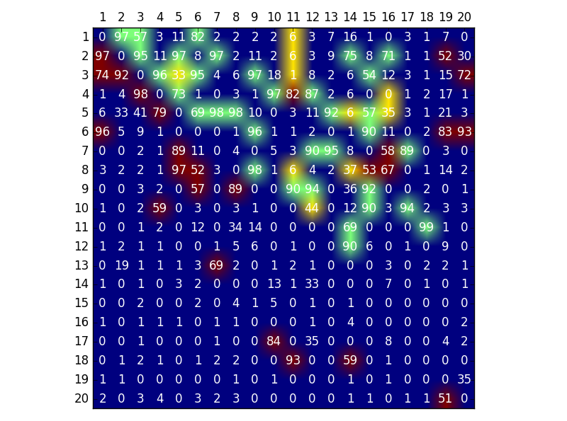
The variability of the results w.r.t. the initialization of both generator and adversarial networks is assessed by considering 100 independent SAM runs on a 20 variable graph with 500 data points generated with multivariate Gaussian process as causal mechanisms (FCM category V, section 5.1).101010The computational training time is 113 seconds on a Nvidia RTX 2080Ti graphic card, with iterations.
Figure 6 displays the confidence scores: the 30 green dots correspond to true positives where over 50% runs rightly select the edge; blue dots correspond to true negatives (less than 50% runs select a wrong edge); the 9 red dots correspond to false positive (more than 50% runs select a wrong edge) and 14 yellow dots correspond to false negative (50% runs fail to select a true edge).
By inspecting a low confidence case (54% runs select the true direction vs 35% for the wrong direction ), the mistakes can be explained as variable has a single parent (Figure 5). As there is no v-structure, SAM can uniquely rely on the functional fit score to orient this edge (like in pairwise methods), which makes the decision more uncertain. Note that due to the DAG penalization constraint, the algorithm cannot choose at the same time and in a same run.


In a word, the algorithm is sensitive to the initialization of the weights. This sensitivity and the variance of the results is addressed by averaging: running SAM multiple times and retaining the edges selected in a majority of runs.
5.4 Impact of the DAG constraint
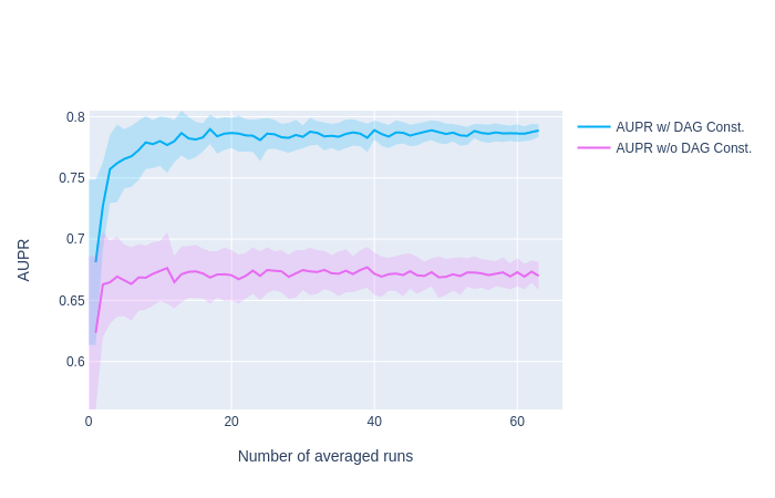
The impact of the DAG constraint is assessed by running SAM with and without the acyclicity penalization constraint (with in the latter case). The experiments consider the same setting as above (section 5.3), and the results are displayed on Figure 9. The average score increases with the number of runs and reaches a plateau, while the variance of the results decreases.
While SAM retrieves almost the same true and false positive edges (respectively in green and yellow), it retrieves a lot more false negative edges (particularly so under the diagonal). This is explained as SAM tends to retrieves the Markov blanket of each node; when there is no DAG constraint, it tends to retrieve edges in both directions, e.g. both and edges are selected almost 100% of the time. Additionally, it tends to retrieve the spouse nodes, e.g. retaining the edge as both nodes have a common child in the true graph (Figure 8).

This edge is not in the true DAG skeleton, but it is in the moralized graph of the true DAG. Therefore, removing the acyclicity constraint (pink curve in Figure 7) increases the number of false positives and degrades the global score.
5.5 Sensitivity to graph density
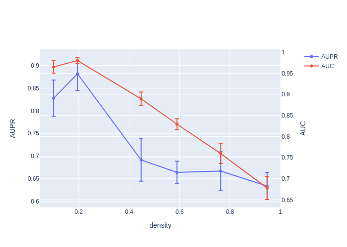
The variability of the results w.r.t. the graph density is assessed by considering 20 variables graphs of different densities with 500 data points and generated with Gaussian process as causal mechanisms (FCM category V, section 5.1).
Figure 10 displays the area under the precision-recall curve and area under the ROC curve (AUPR and AUC, see section 6.3) for different densities of graphs from 0.1 to 0.95.
The best result is obtained for a density of 0.2. It corresponds to an average of almost 2 parents per variable. We observe that this score is better than for a density of 0.1 (with almost 1 parent per variables). It is explained by the fact that with 2 parents per variables there are v-structures which appear, which facilitates the orientation of the edges. Otherwise when the density is greater than 0.2, we observe that the results slightly decrease with the density. There are indeed more edges to recover and it becomes more difficult to find them all.
6 Experimental validation on causal discovery benchmarks
The goal of the validation is to experimentally answer two questions. The first one regards SAM performance compared to the state of the art, depending on whether the underlying joint distribution complies with the usual assumptions (Gaussian distributions for the variables and the noise, linear causal mechanisms). The second question regards the merits and drawbacks of SAM strategy of learning non-linear causal mechanisms, and relying on adversarial learning.
This section first describes different SAM variants used in the experiments, followed by the baseline algorithms and their hyper-parameter settings. Then we describe the performance indicators used in the benchmarks.
Subsection 6.4 reports on the experimental results obtained on synthetic datasets of 20 and 100 variables. Realistic biological data coming from the SynTREN simulator (Van den Bulcke et al., 2006) on 20- and 100-node graphs, and from GeneNetWeaver (Schaffter et al., 2011) on the DREAM4 and DREAM5 challenges are thereafter considered (section 6.5), and we last consider the extensively studied flow cytometry dataset (Sachs et al., 2005) (section 6.6). A t-test is used to assess whether the score difference between any two methods is statistically significant with a p-value 0.001. The detail of all results is given in Appendix D, reporting the average performance indicators, standard deviation, and computational cost of all considered algorithms. A sensitivity analysis to the sample size is given in Appendix E. Appendix F reports a comparison of the SAM algorithm with pairwise methods for the task of Markov equivalence class disambiguation. Finally, an analysis of the robustness of the various methods to non-Gaussian noise is presented in appendix G.
For convenience and reproducibility, all considered algorithms have been integrated in the publicly available CausalDiscovery Toolbox,111111https://github.com/diviyan-kalainathan/causaldiscoverytoolbox. including the most recent baseline versions at the time of the experiments.
6.1 Different SAM variants
In the benchmarks, four variants have been considered: the full SAM (Alg. 1) and three lesioned variants designed to assess the benefits of non-linear mechanisms and adversarial training. Specifically, SAM-lin desactivates the non-linear option and only implements linear causal mechanisms, replacing Equation (11) with:
| (28) |
A second variant, SAM-mse, replaces the adversarial loss with a standard mean-square error loss, replacing the f-gan term in Equation (21) with .
A third variant, SAM-lin-mse, involves both linear mechanisms and mean square error losses.
6.2 Baseline algorithms
The following algorithms have been used, with their default parameters: the score-based methods GES (Chickering, 2002) and GIES (Hauser and Bühlmann, 2012) with Gaussian scores; the hybrid method MMHC (Tsamardinos et al., 2006), the penalized method for causal discovery CCDr (Aragam and Zhou, 2015), the LiNGAM algorithm (Shimizu et al., 2006) and the causal additive model CAM (Peters et al., 2014). Lastly, the PC algorithm (Spirtes et al., 2000) has been considered with four conditional independence tests in the Gaussian and non-parametric settings:
PC,121212The more efficient order-independent version of the PC algorithm proposed by Colombo and Maathuis (2014) is used. GES and LINGAM versions are those of the pcalg package (Kalisch et al., 2012). MMHC is implemented with the bnlearn package (Scutari, 2009). CCDr is implemented with the sparsebn package (Aragam et al., 2017).
The GENIE3 algorithm (Irrthum et al., 2010) is also considered, though it does not focus on DAG discovery per se as it achieves feature selection, retains the Markov Blanket of each variable using random forest algorithms. Nevertheless, this method won the DREAM4 In Silico Multifactorial challenge (Marbach et al., 2009), and is therefore included among the baseline algorithms (using the GENIE3 R package).
6.3 Performance indicators
For the sake of robustness, 16 independent runs have been launched for each dataset-algorithm pair with a bootstrap ratio of 0.8 on the observational samples. The average causation score for each edge is measured as the fraction of runs where this edge belongs to . When an edge is left undirected, e.g with PC algorithm, it is counted as appearing with both orientations with weight .
Area under the Precision Recall Curve (AUPR) and Area under the Receiver Operating Characteristic Curve (AUC)
A true positive is an edge of the true DAG which is correctly recovered by the algorithm; is the number of true positive. A false negative is an edge of which is missing in ; is the number of false negatives. A false positive is an edge in which is not in (reversed edges and edges which are not in the skeleton of ); is the number of false positives. The precision-recall curve, showing the tradeoff between precision () and recall () for different causation thresholds (Figure 14), is summarized by the Area under the Precision Recall Curve (AUPR), ranging in [0,1], with 1 being the optimum. The Receiver Operating Characteristic Curve show the the relationship between the sensitivity () and the specificity (). It can be summarized by the Area under the Receiver Operating Characteristic Curve (AUC) ranging in [0,1], with 1 being the optimum.131313For AUPR and AUC evaluations, we use the scikit-learn v0.20.1 library (Pedregosa et al., 2011).
Structural Hamming Distance
Another performance indicator used in the causal graph discovery framework is the Structural Hamming Distance (SHD) (Tsamardinos et al., 2006), set to the number of missing edges and redundant edges in the found structure. This SHD score is computed in the following by considering all edges with . Note that a reversal error (retaining while includes edge ) is counted as a single mistake.
| (29) |
with (respectively ) the adjacency matrix of (resp. the found causal graph ).
6.4 Experiments on synthetic datasets
We first consider the 6 types of datasets with different causal mechanisms presented in section 5.1.141414The datasets GP AM, GP MIX and Sigmoid AM were considered for the experimental validation of the CAM algorithm (Peters et al., 2014). The synthetic datasets include 10 DAGs with 20 variables and 10 DAGs with 100 variables.
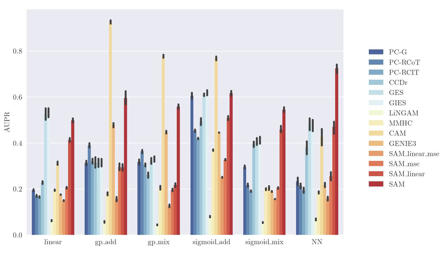
20 variable-graphs
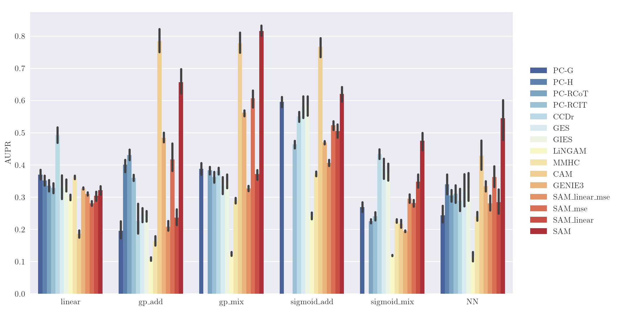
The comparative results (Figure 11) demonstrate SAM robustness in term of Area under the Precision Recall Curve (AUPR) on all categories of 20-node graphs. Specifically, SAM is dominated by PC-G, GES and CCDr on linear mechanisms and by CAM for datasets with additive noise, reminding that PC-G, GES and CCDr (resp. CAM) specifically focuses on linear (resp. additive noise) mechanisms. Note that, while the whole ranking of the algorithms may depend on the considered performance indicator, the best performing algorithm is most often the same regardless of whether the AUPR, the AUC or the Structural Hamming distance is considered. For non-linear cases with complex interactions (the Sigmoid Mix and NN cases), SAM significantly outperforms other non-parametric methods such as PC-HSIC, PC-RCOT and PC-RCIT. In the linear Gaussian setting, SAM aims to the Markov equivalence class of the true graph (under causal Markov and faithfulness assumptions) and performs less well than for e.g. the GP mix where SAM can exploit both conditional independence relations and distribution asymmetries. Though seemingly counter-intuitive, a graph with more complex interactions between noise and variables may be actually easier to recover than a graph generated with simple mechanisms (see also Wang and Blei (2018)).
The SAM computational cost is bigger than for simple linear methods such as GES or PC-Gauss, but often lower than the other non-linear methods such as CAM or PC-HSIC (Table 3 in Appendix D).
The lesioned versions, SAM-lin, SAM-mse and SAM-line-mse have significantly worse performances than SAM (except for the linear mechanism and additive Gaussian noise cases), demonstrating the merits of the NN-based and adversarial learning approach in the general case.
100-variable graphs
The comparative results on the 100-node graphs (Figure 12) confirm the good overall robustness of SAM. As could have been expected, SAM is dominated by CAM on the GP AM, GP Mix and Sigmoid AM settings; indeed, focusing on the proper causal mechanism space yields a significant advantage, all the more so as the number of variables increases. Nevertheless, SAM does never face a catastrophic failure, and it even performs quite well on linear datasets. A tentative explanation is based on the fact that the tanh activation function enables to capture linear mechanisms; another explanation is based on the adversarial loss, empirically more robust than the MSE loss in high-dimensional problems.
In terms of computational cost, SAM scales well at variables even when using a CPU, particularly so when compared to its best competitor CAM, that uses a combinatorial graph search. The PC-HSIC algorithm had to be stopped after 50 hours; more generally, constraint-based methods based on the PC algorithm do not scale well w.r.t. the number of variables, when using costly non-linear conditional independence tests.
6.5 Simulated biological datasets
The SynTREN (Van den Bulcke et al., 2006) and GeneNetWeaver (GNW) (Schaffter et al., 2011) simulators of genetic regulatory networks have been used to generate observational data reflecting realistic complex regulatory mechanisms, high-order conditional dependencies between expression patterns and potential feedback cycles, based on an available causal model.
SynTREN simulator
.
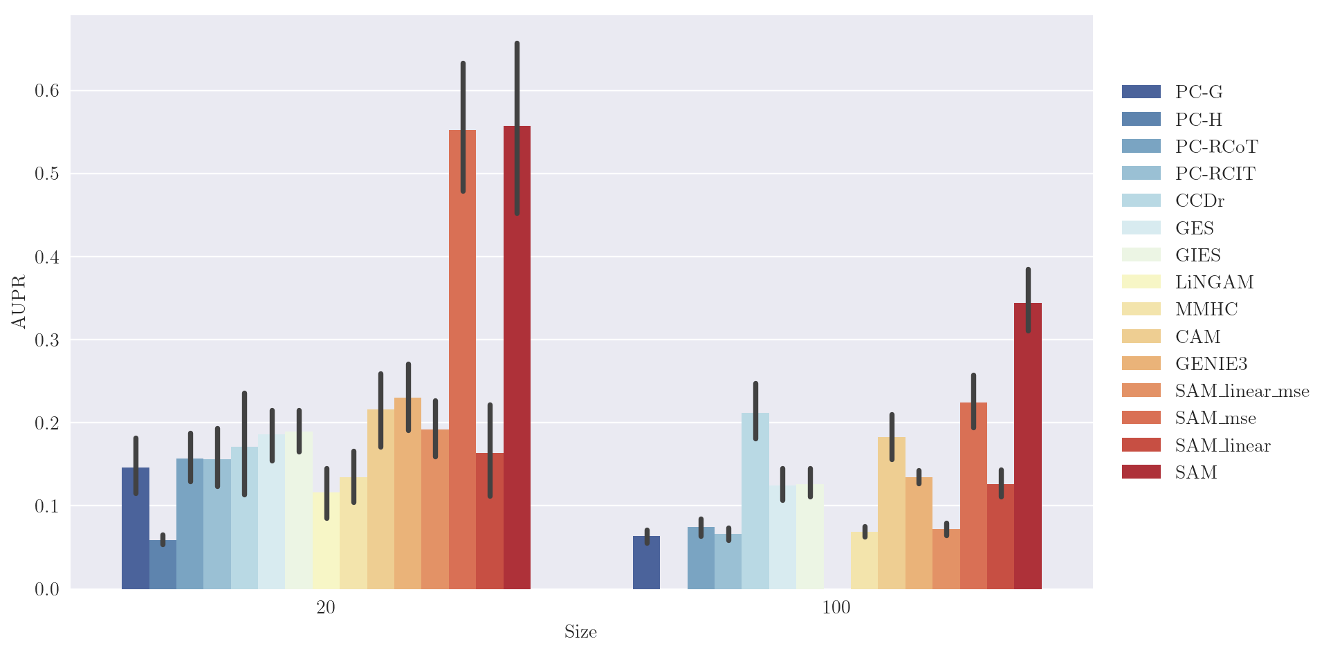
Sub-networks of E. coli (Shen-Orr et al., 2002) have been considered, where interaction kinetics are based on Michaelis-Menten and Hill kinetics (Mendes et al., 2003). Overall, ten 10-nodes and ten 100-nodes graphs have been considered.151515Random seeds set to 110 are used for the sake of reproducibility. SynTREN hyper-parameters include a probability of 1.0 (resp. 0.1) for complex 2-regulator interactions (resp. for biological noise, experimental noise and noise on correlated inputs). For each graph, 500-sample datasets are generated by SynTREN.
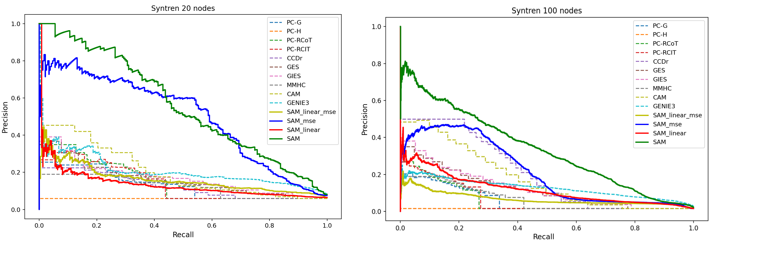
Likewise, the comparative results on all SynTREN graphs (Figure 13) demonstrate the good performances of SAM. Overall, the best performing methods take into account both distribution asymmetry and multivariate interactions. Constraint-based methods are hampered by the lack of v-structures, preventing the orientation of many edges to be based on CI tests only (PC-HSIC algorithm was stopped after 50 hours and LiNGAM did not converge on any of the datasets). The benefits of using non-linear mechanisms on such problems are evidenced by the difference between SAM-lin-mse and SAM-mse (Appendix D). The Precision-Recall curve is displayed on Figure 14 for representative 20-node and 100-node graphs, confirming that SAM can be used to infer networks having complex distributions, complex causal mechanisms and interactions.
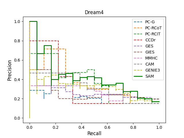
GeneNetWeaver simulator - DREAM4
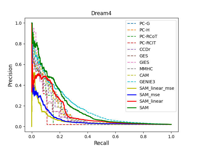
Five 100-nodes graphs generated using the GeneNetWeaver simulator define the In Silico Size 100 Multifactorial challenge track of the Dialogue for Reverse Engineering Assessments and Methods (DREAM) initiative. These graphs are sub-networks of transcriptional regulatory networks of E. coli and S. cerevisiae; their dynamics are simulated using a kinetic gene regulation model, with noise added to both the dynamics of the networks and the measurement of expression data. Multifactorial perturbations are simulated by slightly increasing or decreasing the basal activation of all genes of the network simultaneously by different random amounts. In total, the number of expression conditions for each network is set to 100. As the DREAM 4 graphs contain feedback loops, SAM is launched without the DAG constraint on these instances.
The comparative results on these five graphs (Figure 15) show that GENIE3 outperforms all other methods on networks 1, 2 and 5, while SAM is better on network 3. The Precision/Recall curves (Figure 16) show that SAM is slightly better than GENIE3 in the low recall region, but worst in the high recall region. Overall, on such complex problem domains, it seems preferable to make few assumptions on the underlying generative model (like GENIE3 and SAM), while being able to capture high-order conditional dependencies between variables. Note that LiNGAM did not converge on this Dream4 dataset.
GeneNetWeaver simulator - DREAM5
The largest three networks of the DREAM5 challenge (Marbach et al., 2012) are considered to assess the scalability of SAM. Network 1 is a simulated network with simulated expression data (GeneNetWeaver software), while both other expression datasets are real expression data collected for E. coli (Network 3) and S. cerevisiae (Network 4).161616Note that we do not use in our experiments Network 2 of DREAM5, because no verified interaction is provided for this dataset.
On these datasets, the set of potential causes (Transcription Factors or TF) is known and constitutes a subset of the genes (). The task is to infer all directed edges with and . The ground truth graph is cyclical but self-regulatory relationships are excluded. The number of available transcription factors, genes and observations is displayed on Table 1.
| Network | # TF | # Genes | # Observations | # Verified interactions |
|---|---|---|---|---|
| DREAM5 Network 1 (in-silico) | 195 | 1643 | 805 | 4012 |
| DREAM5 Network 3 (E.coli) | 334 | 4511 | 805 | 2066 |
| DREAM5 Network 4 (S.cerevisiae) | 333 | 5950 | 536 | 3940 |
SAM is adapted to the specifics of the DREAM5 problems by removing the acyclicity constraint (); all other hyperparameters are set to their values used in this section; the edge scores are averaged on 32 runs. SAM is compared with the best results reported by the organizers of the challenge: the Trustful Inference of Gene REgulation using Stability Selection (TIGRESS) (Haury et al., 2012), the Context likelihood of relatedness (CLR) (Faith et al., 2007), the Algorithm for the Reconstruction of Accurate Cellular Networks (ARACNE) (Margolin et al., 2006), the Max-Min Parent and Children algorithm (MMHC) (Tsamardinos et al., 2003), the Markov blanket algorithm (HITON-PC) (Aliferis et al., 2010), the GENIE3 algorithm (Irrthum et al., 2010) and the ANOVA algorithm (Küffner et al., 2012). For SAM and all other methods, the AuPR score is computed with the same evaluation script used in the challenge.171717available at http://dreamchallenges.org.
The results are displayed on Figure 17 (details are given in Table 16, Appendix D). A first remark is that all methods present degraded performance on Networks 3 and 4; a tentative interpretation is that the set of interactions for real data is not always accurate nor complete.
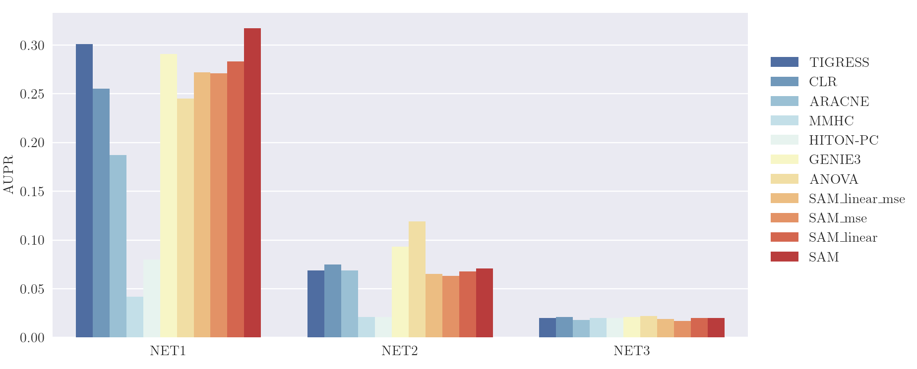
On Network 1, the best results are obtained by SAM, GENIE3 and TIGRESS, with similar performances. A tentative interpretation is that, without the acyclicity constraint, SAM tackles gene regulatory inference through selecting the relevant features to predict each target gene, akin GENIE3 and TIGRESS. The main difference is that GENIE3 aggregates the features selected by regression with decision trees, while TIGRESS aggregates the features selected by LARS.
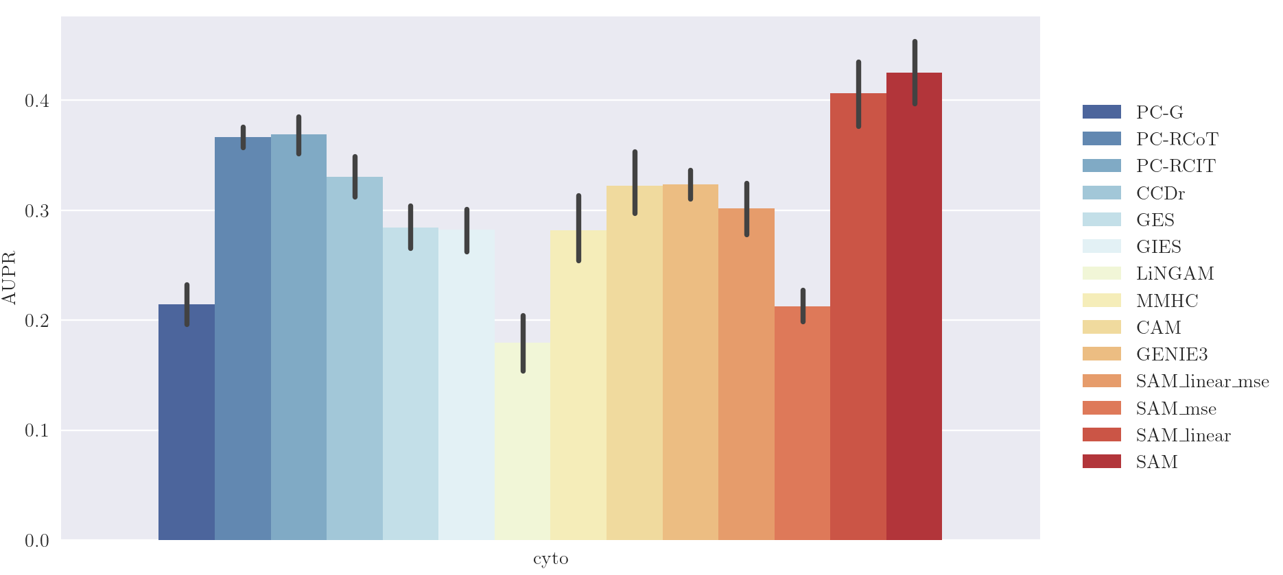
6.6 Real-world biological data
This well-studied protein network problem is associated with gene expression data including 7,466 observational samples for 11 proteins (variables). The signaling molecule causal graph, conventionally accepted as ground truth and used to measure the performance of the different causal discovery methods, is displayed on Figure 18. As this network contains feedback loops, SAM is launched without the acyclicity penalization term on this dataset.

The same experimental setting is used as for the other problems. According to the AUPR indicator (cf. Figure 19 and 20), SAM significantly outperforms the other methods. Notably, SAM recovers the transduction pathway rafmekerk corresponding to direct enzyme-substrate causal effect (Sachs et al., 2005).
7 Discussion and Perspectives
The main contribution of the paper is to propose a new causal discovery method, exploiting both structural independence and distributional asymmetries through optimizing structural and functional criteria. This framework is implemented in the SAM algorithm,181818Available at https://github.com/Diviyan-Kalainathan/SAM. leveraging the representational power of Generative Adversarial Neural networks (GANs) to learn a generative model using stochastic gradient descent, and enforcing the discovery of sparse acyclic causal graphs through adequate regularization terms.
The choices made in the construction of the model (joint log-likelihood estimation of the conditional distributions with the use of an adversarial f-gan neural network; usage of structural, functional and acyclicity constraints) are supported by a theoretical analysis.
In the general case, the identifiability of the causal graph with neural networks as causal mechanisms remains an open question, left for further work. In practice, SAM robustness is supported by extensive empirical evidence across diverse synthetic, realistic and real-world problems, suggesting that SAM can be used as a powerful tool for the practitioner in order to prioritize exploratory experiments when working on real data with no prior information about neither the type of functional mechanisms involved, nor the underlying data distribution.
Lesion studies are conducted to assess whether and when it is beneficial to learn non-linear mechanisms and to rely on adversarial learning as opposed to MSE minimization.
As could have been expected, in particular settings SAM is dominated by algorithms specifically designed for these settings, such as
CAM (Bühlmann et al., 2014) in the case of additive noise model and Gaussian process mechanisms, and GENIE3 when facing causal graphs with feedback loops for some networks. Nevertheless, SAM most often ranks first and always avoids catastrophic failures. SAM has good overall computational efficiency compared to other non-linear methods as it uses an embedded framework for structure optimization, where the mechanisms and the structure are simultaneously learned within an end-to-end DAG learning framework.
It can also easily be trained on a GPU device, thus leveraging on massive parallel computation power available to learn the DAG mechanisms and the adversarial neural network. SAM scalability is demonstrated on the Network 1 of the DREAM5 challenge, obtaining very good performances with a relatively high number of variables (ca 1,500).
This work opens up four avenues for further research. An on-going extension regards the case of categorical and mixed variables, taking inspiration from discrete GANs (Hjelm et al., 2017). Another perspective is to relax the causal sufficiency assumption and handle hidden confounders, e.g. by introducing statistical dependencies between the noise variables attached to different variables (Rothenhäusler et al., 2015), or creating shared noise variables (Janzing and Schölkopf, 2018) or proxies of confounders (Wang and Blei, 2021).
A longer term perspective is to extend SAM to simulate interventions on target variables. Lastly, the case of causal graphs with cycles will be considered, leveraging the power of recurrent neural nets to define a proper generative model from a graph with feedback loops.
Acknowledgment
We would like to thank Dr. Mikael Escobar-Bach for proofreading the paper. This work was granted access to the HPC resources of CCIPL (Nantes, France).
References
- Aliferis et al. (2003) Constantin F Aliferis, Ioannis Tsamardinos, and Alexander Statnikov. Hiton: a novel Markov blanket algorithm for optimal variable selection. In AMIA annual symposium proceedings, volume 2003, page 21. American Medical Informatics Association, 2003.
- Aliferis et al. (2010) Constantin F Aliferis, Alexander Statnikov, Ioannis Tsamardinos, Subramani Mani, and Xenofon D Koutsoukos. Local causal and Markov blanket induction for causal discovery and feature selection for classification part I: Algorithms and empirical evaluation. Journal of Machine Learning Research, 11(1), 2010.
- Aragam and Zhou (2015) Bryon Aragam and Qing Zhou. Concave penalized estimation of sparse gaussian bayesian networks. Journal of Machine Learning Research, 16:2273–2328, 2015.
- Aragam et al. (2017) Bryon Aragam, Jiaying Gu, and Qing Zhou. Learning large-scale bayesian networks with the sparsebn package. arXiv preprint arXiv:1703.04025, 2017.
- Bell and Wang (2000) David A Bell and Hui Wang. A formalism for relevance and its application in feature subset selection. Machine learning, 41(2):175–195, 2000.
- Blöbaum et al. (2018) Patrick Blöbaum, Dominik Janzing, Takashi Washio, Shohei Shimizu, and Bernhard Schölkopf. Cause-effect inference by comparing regression errors. In International Conference on Artificial Intelligence and Statistics, pages 900–909. PMLR, 2018.
- Brown et al. (2012) Gavin Brown, Adam Pocock, Ming-Jie Zhao, and Mikel Luján. Conditional likelihood maximisation: a unifying framework for information theoretic feature selection. Journal of machine learning research, 13(Jan):27–66, 2012.
- Bühlmann et al. (2014) Peter Bühlmann, Jonas Peters, Jan Ernest, et al. Cam: Causal additive models, high-dimensional order search and penalized regression. The Annals of Statistics, 42(6):2526–2556, 2014.
- Chen et al. (2007) Pu Chen, Chihying Hsiao, Peter Flaschel, and Willi Semmler. Causal analysis in economics: Methods and applications. 2007.
- Chickering (2002) David Maxwell Chickering. Optimal structure identification with greedy search. Journal of Machine Learning Research, 2002.
- Chickering (2013) David Maxwell Chickering. A transformational characterization of equivalent bayesian network structures. arXiv preprint arXiv:1302.4938, 2013.
- Colombo and Maathuis (2014) Diego Colombo and Marloes H Maathuis. Order-independent constraint-based causal structure learning. Journal of Machine Learning Research, 2014.
- Colombo et al. (2012) Diego Colombo, Marloes H Maathuis, Markus Kalisch, and Thomas S Richardson. Learning high-dimensional directed acyclic graphs with latent and selection variables. The Annals of Statistics, 2012.
- Daniusis et al. (2012) Povilas Daniusis, Dominik Janzing, Joris Mooij, Jakob Zscheischler, Bastian Steudel, Kun Zhang, and Bernhard Schölkopf. Inferring deterministic causal relations. arXiv, 2012.
- Doshi-Velez and Kim (2017) F. Doshi-Velez and B. Kim. Towards a rigorous science of interpretable machine learning. arXiv:1702.08608, 2017.
- Faith et al. (2007) Jeremiah J Faith, Boris Hayete, Joshua T Thaden, Ilaria Mogno, Jamey Wierzbowski, Guillaume Cottarel, Simon Kasif, James J Collins, and Timothy S Gardner. Large-scale mapping and validation of escherichia coli transcriptional regulation from a compendium of expression profiles. PLoS biol, 5(1):e8, 2007.
- Friedman and Nachman (2000) Nir Friedman and Iftach Nachman. Gaussian process networks. In Proceedings of the Sixteenth Conference on Uncertainty in Artificial Intelligence, UAI’00, page 211–219, San Francisco, CA, USA, 2000. Morgan Kaufmann Publishers Inc. ISBN 1558607099.
- Goodfellow et al. (2014) Ian Goodfellow, Jean Pouget-Abadie, Mehdi Mirza, Bing Xu, David Warde-Farley, Sherjil Ozair, Aaron Courville, and Yoshua Bengio. Generative adversarial nets. Advances in Neural Information Processing Systems, 2014.
- Goudet et al. (2018) Olivier Goudet, Diviyan Kalainathan, Philippe Caillou, Isabelle Guyon, David Lopez-Paz, and Michele Sebag. Learning functional causal models with generative neural networks. In Explainable and Interpretable Models in Computer Vision and Machine Learning, pages 39–80. Springer, 2018.
- Gretton et al. (2005) Arthur Gretton, Ralf Herbrich, Alexander Smola, Olivier Bousquet, and Bernhard Schölkopf. Kernel methods for measuring independence. Journal of Machine Learning Research, 2005.
- Gretton et al. (2007) Arthur Gretton, Karsten M Borgwardt, Malte Rasch, Bernhard Schölkopf, Alexander J Smola, et al. A kernel method for the two-sample-problem. Advances in Neural Information Processing Systems, 2007.
- Guyon et al. (2019) Isabelle Guyon, Alexander Statnikov, and Berna Bakir Batu. Cause Effect Pairs in Machine Learning. Springer International Publishing, 2019. ISBN 978-3-030-21809-6.
- Haury et al. (2012) Anne-Claire Haury, Fantine Mordelet, Paola Vera-Licona, and Jean-Philippe Vert. Tigress: trustful inference of gene regulation using stability selection. BMC systems biology, 6(1):145, 2012.
- Hauser and Bühlmann (2012) Alain Hauser and Peter Bühlmann. Characterization and greedy learning of interventional Markov equivalence classes of directed acyclic graphs. Journal of Machine Learning Research, 13(Aug):2409–2464, 2012.
- Hjelm et al. (2017) R Devon Hjelm, Athul Paul Jacob, Tong Che, Adam Trischler, Kyunghyun Cho, and Yoshua Bengio. Boundary-seeking generative adversarial networks. arXiv preprint arXiv:1702.08431, 2017.
- Hoyer et al. (2009) Patrik O Hoyer, Dominik Janzing, Joris M Mooij, Jonas Peters, and Bernhard Schölkopf. Nonlinear causal discovery with additive noise models. Advances in Neural Information Processing Systems, 2009.
- Hyvärinen and Pajunen (1999) Aapo Hyvärinen and Petteri Pajunen. Nonlinear independent component analysis: Existence and uniqueness results. Neural Networks, 12(3):429–439, 1999.
- Imbens and Rubin (2015) Guido W Imbens and Donald B Rubin. Causal inference in statistics, social, and biomedical sciences. Cambridge University Press, 2015.
- Ioffe and Szegedy (2015) Sergey Ioffe and Christian Szegedy. Batch normalization: Accelerating deep network training by reducing internal covariate shift. In International conference on machine learning, pages 448–456, 2015.
- Irrthum et al. (2010) Alexandre Irrthum, Louis Wehenkel, Pierre Geurts, et al. Inferring regulatory networks from expression data using tree-based methods. PloS one, 5(9):e12776, 2010.
- Jang et al. (2016) Eric Jang, Shixiang Gu, and Ben Poole. Categorical reparameterization with gumbel-softmax. arXiv preprint arXiv:1611.01144, 2016.
- Janzing and Scholkopf (2010) Dominik Janzing and Bernhard Scholkopf. Causal inference using the algorithmic Markov condition. IEEE Transactions on Information Theory, 56(10):5168–5194, 2010.
- Janzing and Schölkopf (2018) Dominik Janzing and Bernhard Schölkopf. Detecting confounding in multivariate linear models via spectral analysis. Journal of Causal Inference, 6(1), 2018.
- Kalisch and Bühlmann (2007) Markus Kalisch and Peter Bühlmann. Estimating high-dimensional directed acyclic graphs with the pc-algorithm. Journal of Machine Learning Research, 8(Mar):613–636, 2007.
- Kalisch et al. (2012) Markus Kalisch, Martin Mächler, Diego Colombo, Marloes H Maathuis, Peter Bühlmann, et al. Causal inference using graphical models with the R package pcalg. Journal of Statistical Software, 2012.
- Karras et al. (2017) Tero Karras, Timo Aila, Samuli Laine, and Jaakko Lehtinen. Progressive growing of GANs for improved quality, stability, and variation. arXiv preprint arXiv:1710.10196, 2017.
- Kingma and Ba (2014) Durk P Kingma and Jimmy Ba. Adam: A Method for Stochastic Optimization. Int. Conf. on Learning Representations, 2014.
- Küffner et al. (2012) Robert Küffner, Tobias Petri, Pegah Tavakkolkhah, Lukas Windhager, and Ralf Zimmer. Inferring gene regulatory networks by anova. Bioinformatics, 28(10):1376–1382, 2012.
- Leray and Gallinari (1999) Philippe Leray and Patrick Gallinari. Feature selection with neural networks. Behaviormetrika, 26(1):145–166, 1999.
- Lopez-Paz and Oquab (2016) David Lopez-Paz and Maxime Oquab. Revisiting classifier two-sample tests. arXiv preprint arXiv:1610.06545, 2016.
- Lopez-Paz et al. (2015) David Lopez-Paz, Krikamol Muandet, Bernhard Schölkopf, and Ilya O Tolstikhin. Towards a learning theory of cause-effect inference. Int. Conf. on Machine Learning, 2015.
- Louizos et al. (2017) Christos Louizos, Max Welling, and Diederik P Kingma. Learning sparse neural networks through regularization. arXiv preprint arXiv:1712.01312, 2017.
- Maddison et al. (2016) Chris J Maddison, Andriy Mnih, and Yee Whye Teh. The concrete distribution: A continuous relaxation of discrete random variables. arXiv preprint arXiv:1611.00712, 2016.
- Marbach et al. (2009) Daniel Marbach, Thomas Schaffter, Dario Floreano, Robert J Prill, and Gustavo Stolovitzky. The dream4 in-silico network challenge. Draft, version 0.3, 2009.
- Marbach et al. (2012) Daniel Marbach, James C Costello, Robert Küffner, Nicole M Vega, Robert J Prill, Diogo M Camacho, Kyle R Allison, Manolis Kellis, James J Collins, and Gustavo Stolovitzky. Wisdom of crowds for robust gene network inference. Nature methods, 9(8):796–804, 2012.
- Margolin et al. (2006) Adam A Margolin, Ilya Nemenman, Katia Basso, Chris Wiggins, Gustavo Stolovitzky, Riccardo Dalla Favera, and Andrea Califano. Aracne: an algorithm for the reconstruction of gene regulatory networks in a mammalian cellular context. In BMC bioinformatics, volume 7, page S7. Springer, 2006.
- Mendes et al. (2003) Pedro Mendes, Wei Sha, and Keying Ye. Artificial gene networks for objective comparison of analysis algorithms. Bioinformatics, 19(suppl_2):ii122–ii129, 2003.
- Mirza and Osindero (2014) Mehdi Mirza and Simon Osindero. Conditional generative adversarial nets. arXiv, 2014.
- Mooij et al. (2010) Joris M Mooij, Oliver Stegle, Dominik Janzing, Kun Zhang, , and Bernhard Schölkopf. Probabilistic latent variable models for distinguishing between cause and effect. Advances in Neural Information Processing Systems, 2010.
- Mooij et al. (2016) Joris M Mooij, Jonas Peters, Dominik Janzing, Jakob Zscheischler, and Bernhard Schölkopf. Distinguishing cause from effect using observational data: methods and benchmarks. Journal of Machine Learning Research, 2016.
- Nandy et al. (2015) Preetam Nandy, Alain Hauser, and Marloes H Maathuis. High-dimensional consistency in score-based and hybrid structure learning. arXiv, 2015.
- Neyshabur et al. (2017) Behnam Neyshabur, Srinadh Bhojanapalli, David McAllester, and Nati Srebro. Exploring generalization in deep learning. In Advances in Neural Information Processing Systems, pages 5947–5956, 2017.
- Nguyen et al. (2010) XuanLong Nguyen, Martin J Wainwright, and Michael I Jordan. Estimating divergence functionals and the likelihood ratio by convex risk minimization. IEEE Transactions on Information Theory, 56(11):5847–5861, 2010.
- Nowozin et al. (2016) Sebastian Nowozin, Botond Cseke, and Ryota Tomioka. f-gan: Training generative neural samplers using variational divergence minimization. In Advances in Neural Information Processing Systems, pages 271–279, 2016.
- Ogarrio et al. (2016) Juan Miguel Ogarrio, Peter Spirtes, and Joe Ramsey. A hybrid causal search algorithm for latent variable models. Conference on Probabilistic Graphical Models, 2016.
- Pearl (2003) Judea Pearl. Causality: models, reasoning, and inference. Econometric Theory, 19(675-685):46, 2003.
- Pearl (2009) Judea Pearl. Causality. 2009.
- Pearl and Verma (1991) Judea Pearl and Thomas Verma. A formal theory of inductive causation. 1991.
- Pedregosa et al. (2011) F. Pedregosa, G. Varoquaux, A. Gramfort, V. Michel, B. Thirion, O. Grisel, M. Blondel, P. Prettenhofer, R. Weiss, V. Dubourg, J. Vanderplas, A. Passos, D. Cournapeau, M. Brucher, M. Perrot, and E. Duchesnay. Scikit-learn: Machine learning in Python. Journal of Machine Learning Research, 12:2825–2830, 2011.
- Peters et al. (2014) Jonas Peters, Joris M Mooij, Dominik Janzing, and Bernhard Schölkopf. Causal discovery with continuous additive noise models. The Journal of Machine Learning Research, 15(1):2009–2053, 2014.
- Peters et al. (2017) Jonas Peters, Dominik Janzing, and Bernhard Schölkopf. Elements of Causal Inference - Foundations and Learning Algorithms. MIT Press, 2017.
- Quinn et al. (2011) John A Quinn, Joris M Mooij, Tom Heskes, and Michael Biehl. Learning of causal relations. ESANN, 2011.
- Ramsey et al. (2017) Joseph Ramsey, Madelyn Glymour, Ruben Sanchez-Romero, and Clark Glymour. A million variables and more: the fast greedy equivalence search algorithm for learning high-dimensional graphical causal models, with an application to functional magnetic resonance images. International journal of data science and analytics, 3(2):121–129, 2017.
- Ramsey (2015) Joseph D Ramsey. Scaling up greedy causal search for continuous variables. arXiv, 2015.
- Rothenhäusler et al. (2015) Dominik Rothenhäusler, Christina Heinze, Jonas Peters, and Nicolai Meinshausen. Backshift: Learning causal cyclic graphs from unknown shift interventions. In Advances in Neural Information Processing Systems, pages 1513–1521, 2015.
- Sachs et al. (2005) Karen Sachs, Omar Perez, Dana Pe’er, Douglas A Lauffenburger, and Garry P Nolan. Causal protein-signaling networks derived from multiparameter single-cell data. Science, 308(5721):523–529, 2005.
- Schaffter et al. (2011) Thomas Schaffter, Daniel Marbach, and Dario Floreano. Genenetweaver: in silico benchmark generation and performance profiling of network inference methods. Bioinformatics, 27(16):2263–2270, 2011.
- Scutari (2009) Marco Scutari. Learning bayesian networks with the bnlearn r package. arXiv, 2009.
- Shen-Orr et al. (2002) Shai S Shen-Orr, Ron Milo, Shmoolik Mangan, and Uri Alon. Network motifs in the transcriptional regulation network of escherichia coli. Nature genetics, 31(1):64, 2002.
- Shimizu et al. (2006) Shohei Shimizu, Patrik O Hoyer, Aapo Hyvärinen, and Antti Kerminen. A linear non-gaussian acyclic model for causal discovery. Journal of Machine Learning Research, 2006.
- Spirtes and Zhang (2016) Peter Spirtes and Kun Zhang. Causal discovery and inference: concepts and recent methodological advances. Applied informatics, 2016.
- Spirtes et al. (1993) Peter Spirtes, Clark Glymour, and Richard Scheines. Causation, prediction and search. 1993. Lecture Notes in Statistics, 1993.
- Spirtes et al. (2000) Peter Spirtes, Clark N Glymour, and Richard Scheines. Causation, prediction, and search. 2000.
- Srivastava et al. (2014) Nitish Srivastava, Geoffrey Hinton, Alex Krizhevsky, Ilya Sutskever, and Ruslan Salakhutdinov. Dropout: a simple way to prevent neural networks from overfitting. The Journal of Machine Learning Research, 15(1):1929–1958, 2014.
- Statnikov et al. (2012) Alexander Statnikov, Mikael Henaff, Nikita I Lytkin, and Constantin F Aliferis. New methods for separating causes from effects in genomics data. BMC genomics, 2012.
- Strobl et al. (2017) Eric V Strobl, Kun Zhang, and Shyam Visweswaran. Approximate kernel-based conditional independence tests for fast non-parametric causal discovery. arXiv preprint arXiv:1702.03877, 2017.
- Tsamardinos et al. (2003) Ioannis Tsamardinos, Constantin F. Aliferis, and Alexander Statnikov. Time and sample efficient discovery of Markov blankets and direct causal relations. In Proceedings of the ninth ACM SIGKDD international conference on Knowledge discovery and data mining, pages 673–678, 2003.
- Tsamardinos et al. (2006) Ioannis Tsamardinos, Laura E Brown, and Constantin F Aliferis. The max-min hill-climbing bayesian network structure learning algorithm. Machine learning, 65(1):31–78, 2006.
- Van den Bulcke et al. (2006) Tim Van den Bulcke, Koenraad Van Leemput, Bart Naudts, Piet van Remortel, Hongwu Ma, Alain Verschoren, Bart De Moor, and Kathleen Marchal. Syntren: a generator of synthetic gene expression data for design and analysis of structure learning algorithms. BMC bioinformatics, 7(1):43, 2006.
- Vergara and Estévez (2014) Jorge R. Vergara and Pablo A. Estévez. A review of feature selection methods based on mutual information. Neural computing and applications, 24(1):175–186, 2014.
- Wang and Blei (2018) Yixin Wang and David M. Blei. The blessings of multiple causes. CoRR, abs/1805.06826, 2018. URL http://arxiv.org/abs/1805.06826.
- Wang and Blei (2021) Yixin Wang and David M. Blei. A proxy variable view of shared confounding. In Marina Meila and Tong Zhang, editors, Proceedings of the 38th International Conference on Machine Learning, ICML 2021, 18-24 July 2021, Virtual Event, volume 139 of Proceedings of Machine Learning Research, pages 10697–10707. PMLR, 2021.
- Yu et al. (2018) Kui Yu, Lin Liu, and Jiuyong Li. A unified view of causal and non-causal feature selection. arXiv preprint arXiv:1802.05844, 2018.
- Zhang and Hyvärinen (2010) Kun Zhang and Aapo Hyvärinen. Distinguishing causes from effects using nonlinear acyclic causal models. In Causality: Objectives and Assessment, pages 157–164, 2010.
- Zhang et al. (2012) Kun Zhang, Jonas Peters, Dominik Janzing, and Bernhard Schölkopf. Kernel-based conditional independence test and application in causal discovery. arXiv, 2012.
- Zheng et al. (2018) Xun Zheng, Bryon Aragam, Pradeep Ravikumar, and Eric P. Xing. Dags with NO TEARS: continuous optimization for structure learning. In Advances in Neural Information Processing Systems (NeurIPS), pages 9492–9503, 2018.
Appendices
Appendix A Notations and definitions
| Notation | Definition |
|---|---|
| X | Set of continuous random variables |
| Set of all continuous random variables in X except and | |
| iid -sample of X | |
| -th sample of | |
| True marginal probability density function of | |
| True conditional probability density function of conditionally to | |
| True joint probability density function of X | |
| Generated marginal probability density function for | |
| Generated conditional probability density function of conditionally to | |
| Generated joint probability density function for X | |
| True causal graph associated to X; is both a continuous random variable and a node in | |
| Candidate causal graph | |
| Total number of edges in | |
| Set of parents of the node in | |
| Set of variables that are not parents of in nor itself | |
| Entropy of variable | |
| Mutual Information between and | |
| Conditional mutual Information between and conditionally to | |
| Pearson correlation coefficient between and | |
| Kullback-Leibler Divergence between the joint probability density functions and of | |
| Set of parameters of a SAM (except the functional and structural gates , ) | |
| Optimal set of parameters of a SAM, that minimises the loss in a given configuration | |
| Regularization weight of the structural complexity of the model. | |
| Regularization weight of the functional complexity of the model. | |
| Regularization weight of the acyclicity constraint term. | |
| Variables and are independent conditionally to all other variables in X | |
| Markov blanket of the variable (node) | |
| Covariance matrix of X | |
| Covariance matrix of | |
| Precision matrix of X | |
| FCM | Functional Causal Model |
| DAG | Directed Acyclic Graph |
| CPDAG | Completed Partially Directed Acyclic Graph |
| CMA | Causal Markov Assumption |
| CFA | Causal Faithfulness Assumption |
| CSA | Causal Sufficiency Assumption |
Appendix B Structural loss: Proof of Theorem 1 and example
Theororem 1 : DAG identification up to the Markov equivalence class
If we assume CMA, CFA and CSA:
i) For every DAG in the equivalence class of , converges to zero in probability when tends to infinity.
ii) For every DAG not in the equivalence class of , there exists such that
goes toward 1 when tends to infinity.
Proof
i) According to Chickering (2013) (Theorem 2), for every DAG in the equivalence class of , there exists a sequence of distinct edge reversals in with the following properties:
-
•
Each edge reversed in is a covered edge (an edge is said covered in if ).
-
•
After each reversal, is a DAG and is equivalent to .
-
•
After all reversals, .
Let be defined from by reversing a single covered edge .
Let us compare the two quantities and :
By definition of a covered edge, we have and after the edge reversal in , and . Then:
Therefore for every DAG in the equivalence class of there is a sequence of covered edge reversals that do not change the global conditional mutual information score and such that after all reversals , thus .
Therefore, for every DAG in the equivalence class of , if we now compare the structural losses of and , we obtain :
We know that and , thus we obtain:
As converges toward in probability for any graph , it gives the result.
ii) a) Consider some graph that implies an independence assumption that does not support. We must have:
| (30) |
Therefore,
Therefore, converges toward in probability.
Since corresponds to more independence assumptions than , there is a lower number of edges in than in . If is chosen such that , then . Thus, goes toward 1 when tends to infinity.
b) Now, if we assume that implies all the independence assumptions in , but that implies an independence assumption that does not, we have:
| (31) |
Therefore, converges toward in probability. Now, since corresponds to fewer independence assumptions than , there is a higher number of edges in than in . Thus, . Then, goes toward 1 when tends to infinity.
Both results i) and ii) establish the consistency of the structural loss .
Theoretical illustration with three variables DAGs
A toy example with three variables , and is used to show that the structural loss may lead to identify the proper orientation of causal edges, based on the Markov property of the data distribution. We assume that the associated graph skeleton is .
In the large sample limit, if we remove the structural penalty for simplicity, as all DAGs have the same number of edges, for each of the four possible DAGs from this skeleton the structural scores are191919We use the formula :
Thus, we have as the three DAGs , and are Markov equivalent.
The difference of score between the two equivalent classes and is
Therefore, if and then and the structure v-structure is preferred. However if and , and the equivalence class is preferred.
Experimental illustration
Let us consider the three variables , assuming linear dependency and Gaussian noise (therefore only conditional independence can be used to orient the edges (Shimizu et al., 2006; Hoyer et al., 2009)).
The four possible DAGs based on this skeleton are used to generate 2,000 sample datasets, where the noise variables are independently sampled from . The experiments are conducted using SAM-lin (section 5.2) to avoid the structural regularization impact; the data fitting loss measured by the discriminator is averaged over 128 independent runs.
The overall loss associated to all candidate structures, respectively denoted: i) and for the chain structures and ; ii) for the V structure ; iii) for the reversed V structure are reported on Figure 21 in the case where the true causal graph is a v-structure, showing that the structural loss indeed enables to statistically significantly identify the true v-structure with as few as 100 examples.
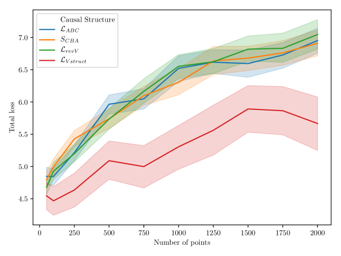
Appendix C Parametric loss : illustration of Markov equivalence class disambiguation
Let us consider the 2-variable toy dataset (Figure 22), where all candidate structures lie in the Markov equivalence class :
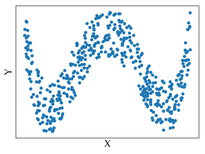
The 500 sample dataset generated after the above FCM was processed using SAM (section 5). The overall average Frobenius regularization loss (in blue) and the total fit loss of the two generators (in red) and for the two models (solid lines) and (dashed lines) are displayed on Figure 23 for different values of the functional regularization parameter (average results on 32 runs). The error bars corresponds to the standard deviation.
Note that simple tests cannot be used to disambiguate the sought causal graph in its Markov equivalence class: the Pearson coefficient is 0 as non-linear models are needed to explain the relation between both variables, conditional independences do not apply as only 2 variables are considered.
However, for all values of both the Frobenius regularization loss and the fit loss are lower for the model than for the model and the difference is statistically significant (t-test with p-value 0.001).
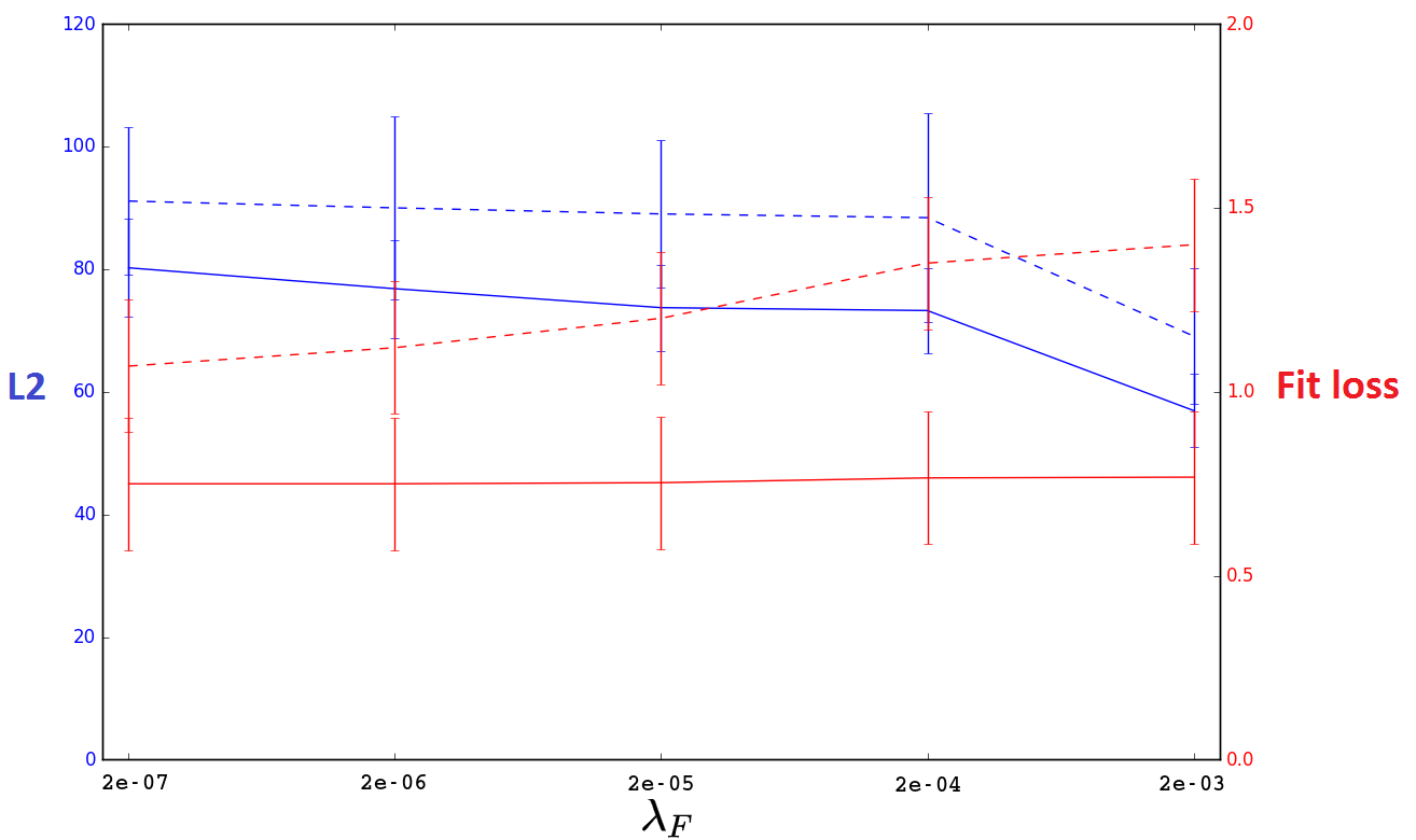
Appendix D Detail of the experimental results
This Appendix details the experimental results reported in section 6. CPU computational times are measured on a 48-core Intel(R) Xeon(R) CPU E5-2650 CPU. For SAM, GPU computational times are measured on a Nvidia RTX 2080Ti GPU.
As the results of the algorithms reported in this table where obtain using different programming languages, the timing information is provided for indicative purposes only. We also mention that other methods such as PC-HSIC, PC-RCOT or PC-RCIT are mostly matrix operations which could benefit greatly from being computed on a GPU.
20-variable artificial graphs
Tables 3,4 and 5 show the robustness of SAM w.r.t. diverse types of mechanisms. In terms of average precision (Table 3) SAM is respectively dominated on linear (resp. CAM on GP AM and Sigmoid AM) mechanisms, which is explained as GES (resp. CAM) is specifically designed to identify linear (resp. additive noise) causal mechanisms.
| AUPR | Linear | GP AM | GP Mix | Sigmoid AM | Sigmoid Mix | NN | Global | CPU Time | GPU Time in s. |
| PC-Gauss | 0.37 (0.02) | 0.20 (0.04) | 0.39 (0.03) | 0.60 (0.03) | 0.27 (0.02) | 0.24 (0.04) | 0.34 (0.14) | 1 | |
| PC-HSIC | 0.35 (0.02) | 0.41 (0.06) | 0.38 (0.03) | 0.41 (0.04) | 0.27 (0.03) | 0.34 (0.05) | 0.36 (0.05) | 46,523 | |
| PC-RCOT | 0.34 (0.03) | 0.43 (0.03) | 0.38 (0.02) | 0.36 (0.05) | 0.23 (0.01) | 0.31 (0.03) | 0.34 (0.07) | 356 | |
| PC-RCIT | 0.33 (0.03) | 0.36 (0.02) | 0.36 (0.03) | 0.46 (0.02) | 0.24 (0.02) | 0.31 (0.05) | 0.34 (0.07) | 181 | |
| GES | 0.33 (0.06) | 0.25 (0.03) | 0.34 (0.04) | 0.58 (0.05) | 0.39 (0.05) | 0.32 (0.08) | 0.37 (0.12) | 1 | |
| GIES | 0.34 (0.03) | 0.24 (0.03) | 0.35 (0.04) | 0.58 (0.05) | 0.38 (0.04) | 0.33 (0.07) | 0.37 (0.11) | 1 | |
| MMHC | 0.36 (0.01) | 0.16 (0.02) | 0.29 (0.01) | 0.37 (0.01) | 0.23 (0.01) | 0.24 (0.02) | 0.28 (0.08) | 1 | |
| LiNGAM | 0.30 (0.02) | 0.11 (0.01) | 0.12 (0.01) | 0.24 (0.02) | 0.12 (0.01) | 0.11 (0.02) | 0.17 (0.08) | 2 | |
| CAM | 0.19 (0.02) | 0.78 (0.06) | 0.78 (0.05) | 0.77 (0.05) | 0.22 (0.02) | 0.43 (0.08) | 0.53 (0.27) | 2,880 | |
| CCDr | 0.49 (0.04) | 0.23 (0.07) | 0.38 (0.02) | 0.55 (0.02) | 0.43 (0.03) | 0.29 (0.06) | 0.40 (0.12) | 2 | |
| GENIE3 | 0.33 (0.01) | 0.48 (0.02) | 0.56 (0.01) | 0.47 (0.01) | 0.19 (0.01) | 0.33 (0.03) | 0.40 (0.12) | 54 | |
| SAM-lin-mse | 0.31 (0.01) | 0.21 (0.03) | 0.33 (0.01) | 0.41 (0.02) | 0.30 (0.02) | 0.28 (0.04) | 0.30 (0.06) | 332 | 70 |
| SAM-mse | 0.28 (0.01) | 0.42 (0.07) | 0.61 (0.04) | 0.52 (0.02) | 0.28 (0.02) | 0.36 (0.05) | 0.41 (0.13) | 2,411 | 83 |
| SAM-lin | 0.30 (0.02) | 0.24 (0.04) | 0.37 (0.02) | 0.50 (0.03) | 0.35 (0.03) | 0.28 (0.06) | 0.34 (0.09) | 2,526 | 110 |
| SAM | 0.32 (0.02) | 0.66 (0.06) | 0.82 (0.03) | 0.62 (0.04) | 0.48 (0.04) | 0.55 (0.10) | 0.57 (0.16) | 13,121 | 113 |
| AUC | Linear | GP AM | GP Mix | Sigmoid AM | Sigmoid Mix | NN | Global |
|---|---|---|---|---|---|---|---|
| PC-Gauss | 0.75 (0.01) | 0.61 (0.03) | 0.71 (0.01) | 0.82 (0.01) | 0.68 (0.02) | 0.65 (0.03) | 0.70 (0.07) |
| PC-HSIC | 0.74 (0.02) | 0.76 (0.03) | 0.69 (0.02) | 0.72 (0.03) | 0.68 (0.02) | 0.71 (0.02) | 0.72 (0.06) |
| PC-RCOT | 0.73 (0.02) | 0.76 (0.02) | 0.76 (0.02) | 0.75 (0.03) | 0.63 (0.01) | 0.71 (0.02) | 0.72 (0.05) |
| PC-RCIT | 0.73 (0.02) | 0.73 (0.01) | 0.75 (0.02) | 0.79 (0.02) | 0.64 (0.03) | 0.72 (0.03) | 0.73 (0.05) |
| GES | 0.77 (0.03) | 0.74 (0.04) | 0.75 (0.03) | 0.87 (0.03) | 0.84 (0.03) | 0.76 (0.07) | 0.79 (0.06) |
| GIES | 0.77 (0.03) | 0.75 (0.03) | 0.76 (0.03) | 0.87 (0.03) | 0.84 (0.03) | 0.76 (0.07) | 0.79 (0.06) |
| MMHC | 0.80 (0.01) | 0.59 (0.03) | 0.72 (0.01) | 0.81 (0.01) | 0.67 (0.02) | 0.67 (0.04) | 0.71 (0.08) |
| LiNGAM | 0.62 (0.01) | 0.44 (0.04) | 0.50 (0.02) | 0.61 (0.02) | 0.43 (0.02) | 0.45 (0.04) | 0.51 (0.09) |
| CAM | 0.65 (0.02) | 0.96 (0.02) | 0.94 (0.01) | 0.94 (0.02) | 0.72 (0.02) | 0.80 (0.05) | 0.83 (0.12) |
| CCDr | 0.82 (0.02) | 0.66 (0.06) | 0.68 (0.02) | 0.80 (0.01) | 0.82 (0.02) | 0.69 (0.07) | 0.74 (0.08) |
| GENIE3 | 0.77 (0.01) | 0.85 (0.01) | 0.92 (0.01) | 0.89 (0.01) | 0.65 (0.01) | 0.78 (0.04) | 0.81 (0.09) |
| SAM-lin-mse | 0.81 (0.01) | 0.70 (0.02) | 0.73 (0.03) | 0.85 (0.01) | 0.79 (0.01) | 0.74 (0.03) | 0.77 (0.05) |
| SAM-mse | 0.80 (0.01) | 0.84 (0.02) | 0.87 (0.02) | 0.90 (0.01) | 0.80 (0.01) | 0.80 (0.03) | 0.83 (0.04) |
| SAM-lin | 0.77 (0.02) | 0.69 (0.02) | 0.75 (0.02) | 0.83 (0.02) | 0.79 (0.02) | 0.74 (0.04) | 0.76 (0.05) |
| SAM | 0.76 (0.02) | 0.90 (0.02) | 0.95 (0.01) | 0.90 (0.01) | 0.85 (0.01) | 0.86 (0.04) | 0.87 (0.06) |
| SHD | Linear | GP AM | GP Mix | Sigmoid AM | Sigmoid Mix | NN | Global |
|---|---|---|---|---|---|---|---|
| PC-Gauss | 37.4 (1.0) | 57.9 (4.0) | 41.4 (2.2) | 26.6 (1.7) | 46.5 (2.1) | 47.4 (2.0) | 42.9 (9.9) |
| PC-HSIC | 38.8 (2.0) | 42.9 (3.1) | 41.7 (5.2) | 41.3 (2.2) | 47.5 (3.3) | 40.7 (2.0) | 42.1 (6.1) |
| PC-RCOT | 40.0 (1.4) | 42.8 (3.2) | 42.6 (1.8) | 43.1 (2.1) | 44.1 (0.5) | 41.7 (2.1) | 42.4 (2.4) |
| PC-RCIT | 40.1 (1.2) | 46.9 (1.8) | 44.9 (1.7) | 34.7 (1.1) | 43.8 (0.5) | 41.6 (1.8) | 41.9 (4.2) |
| GES | 59.2 (5.3) | 70.7 (5.4) | 50.2 (3.5) | 36.0 (3.8) | 58.6 (6.8) | 67.3 (10.8) | 57.0 (13.1) |
| GIES | 60.8 (4.7) | 71.7 (4.9) | 50.3 (3.9) | 35.4 (2.9) | 61.0 (5.1) | 69.1 (10.1) | 58.0 (13.5) |
| MMHC | 41.9 (1.4) | 73.8 (5.0) | 56.2 (1.9) | 46.4 (1.2) | 53.1 (1.3) | 47.8 (2.7) | 53.2 (10.6) |
| LiNGAM | 40.8 (2.2) | 51.3 (1.6) | 48.3 (0.5) | 42.2 (0.9) | 51.0 (2.0) | 55.9 (7.3) | 48.3 (6.2) |
| CAM | 79.4 (6.7) | 37.4 (6.0) | 38.3 (4.3) | 37.4 (4.5) | 85.1 (4.3) | 61.4 (6.9) | 56.5 (20.9) |
| CCDr | 66.2 (6.2) | 57.0 (5.6) | 39.0 (1.6) | 28.4 (2.7) | 40.4 (1.9) | 57.3 (9.8) | 48.0 (14.2) |
| GENIE3 | 41.1 (3.6) | 42.5 (2.9) | 43.2 (4.1) | 41.8 (3.5) | 43.9 (5.2) | 69.2 (9.2) | 47.0 (6.9) |
| SAM-lin-mse | 45.2 (1.1) | 52.5 (2.3) | 44.8 (1.1) | 42.1 (1.4) | 45.8 (1.7) | 42.7 (1.5) | 45.5 (3.7) |
| SAM-mse | 47.9 (1.6) | 46.6 (4.5) | 34.7 (2.5) | 37.2 (2.9) | 53.1 (1.7) | 43.7 (3.0) | 43.9 (6.9) |
| SAM-lin | 42.3 (2.3) | 57.1 (3.9) | 50.3 (3.7) | 42.8 (3.9) | 45.2 (2.3) | 47.3 (4.0) | 47.5 (6.1) |
| SAM | 44.0 (2.1) | 33.9 (4.8) | 21.8 (2.9) | 34.3 (2.8) | 43.6 (2.5) | 37.6 (4.6) | 35.9 (8.2) |
100-variable artificial graphs
Tables 6, and 8 show the scalability of SAM w.r.t. the number of variables. In terms of AUPR precision (Table 6), SAM is dominated by CAM on the GP AM, GP Mix and Sigmoid AM causal mechanisms (noting that CAM is tailored to Gaussian Processes). Most interestingly, its computational time favorably compares to that of CAM on 100-variable problems. Note that PC-HSIC had to be stopped after 50 hours.
| AUPR | Linear | GP AM | GP Mix | Sigmoid AM | Sigmoid Mix | NN | Global | CPU Time | GPU Time |
| PC-Gauss | 0.19 (0.01) | 0.31 (0.02) | 0.32 (0.02) | 0.61 (0.02) | 0.30 (0.01) | 0.23 (0.03) | 0.33 (0.13) | 13 | |
| PC-HSIC | - | - | - | - | - | - | - | - | |
| PC-RCOT | 0.18 (0.01) | 0.39 (0.02) | 0.36 (0.01) | 0.45 (0.01) | 0.22 (0.01) | 0.21 (0.02) | 0.30 (0.11) | 31,320 | |
| PC-RCIT | 0.17 (0.01) | 0.32 (0.02) | 0.31 (0.01) | 0.52 (0.01) | 0.19 (0.01) | 0.19 (0.02) | 0.27 (0.09) | 46,440 | |
| GES | 0.53 (0.04) | 0.32 (0.03) | 0.32 (0.02) | 0.61 (0.01) | 0.41 (0.03) | 0.48 (0.04) | 0.44 (0.11) | 1 | |
| GIES | 0.53 (0.03) | 0.31 (0.03) | 0.33 (0.02) | 0.62 (0.02) | 0.41 (0.02) | 0.48 (0.04) | 0.45 (0.11) | 5 | |
| MMHC | 0.20 (0.01) | 0.18 (0.01) | 0.21 (0.01) | 0.37 (0.01) | 0.20 (0.01) | 0.19 (0.01) | 0.22 (0.07) | 5 | |
| LiNGAM | 0.06 (0.01) | 0.06 (0.01) | 0.04 (0.01) | 0.08 (0.01) | 0.05 (0.01) | 0.07 (0.01) | 0.06 (0.01) | 5 | |
| CAM | 0.31 (0.01) | 0.93 (0.01) | 0.78 (0.01) | 0.77 (0.01) | 0.20 (0.01) | 0.43 (0.05) | 0.57 (0.28) | 45,899 | |
| CCDr | 0.23 (0.01) | 0.31 (0.04) | 0.26 (0.02) | 0.49 (0.02) | 0.39 (0.02) | 0.38 (0.05) | 0.35 (0.09) | 3 | |
| GENIE3 | 0.18 (0.01) | 0.48 (0.02) | 0.45 (0.01) | 0.45 (0.01) | 0.19 (0.01) | 0.22 (0.02) | 0.33 (0.13) | 511 | |
| SAM-lin-mse | 0.15 (0.003) | 0.16 (0.02) | 0.13 (0.01) | 0.25 (0.004) | 0.16 (0.002) | 0.16 (0.01) | 0.17 (0.04) | 3,076 | 74 |
| SAM-mse | 0.21 (0.01) | 0.30 (0.03) | 0.20 (0.01) | 0.33 (0.005) | 0.20 (0.01) | 0.26 (0.03) | 0.25 (0.05) | 12,896 | 118 |
| SAM-lin | 0.41 (0.01) | 0.29 (0.02) | 0.22 (0.01) | 0.51 (0.01) | 0.46 (0.02) | 0.47 (0.04) | 0.39 (0.11) | 8,746 | 516 |
| SAM | 0.50 (0.02) | 0.60 (0.04) | 0.56 (0.02) | 0.62 (0.02) | 0.55 (0.02) | 0.72 (0.03) | 0.59 (0.08) | 15,361 | 519 |
| AUC | Linear | GP AM | GP Mix | Sigmoid AM | Sigmoid Mix | NN | Global |
|---|---|---|---|---|---|---|---|
| PC-Gauss | 0.66 (0.005) | 0.74 (0.01) | 0.74 (0.01) | 0.88 (0.01) | 0.71 (0.01) | 0.68 (0.01) | 0.73 (0.07) |
| PC-HSIC | - | - | - | - | - | - | - |
| PC-RCOT | 0.66 (0.01) | 0.79 (0.01) | 0.77 (0.01) | 0.82 (0.01) | 0.69 (0.01) | 0.68 (0.01) | 0.73 (0.06) |
| PC-RCIT | 0.65 (0.01) | 0.76 (0.01) | 0.74 (0.01) | 0.80 (0.01) | 0.67 (0.01) | 0.67 (0.01) | 0.72 (0.05) |
| GES | 0.92 (0.01) | 0.87 (0.01) | 0.81 (0.01) | 0.94 (0.01) | 0.89 (0.01) | 0.91 (0.01) | 0.89 (0.04) |
| GIES | 0.92 (0.01) | 0.87 (0.01) | 0.81 (0.01) | 0.95 (0.01) | 0.90 (0.01) | 0.91 (0.01) | 0.89 (0.04) |
| MMHC | 0.69 (0.01) | 0.74 (0.01) | 0.75 (0.01) | 0.89 (0.01) | 0.71 (0.01) | 0.69 (0.005) | 0.75 (0.07) |
| LiNGAM | 0.49 (0.01) | 0.49 (0.01) | 0.50 (0.01) | 0.49 (0.01) | 0.51 (0.01) | 0.50 (0.02) | 0.50 (0.01) |
| CAM | 0.77 (0.01) | 0.99 (0.003) | 0.95 (0.01) | 0.96 (0.01) | 0.79 (0.01) | 0.85 (0.02) | 0.89 (0.09) |
| CCDr | 0.75 (0.01) | 0.75 (0.02) | 0.66 (0.02) | 0.80 (0.02) | 0.81 (0.01) | 0.80 (0.02) | 0.76 (0.06) |
| GENIE3 | 0.76 (0.01) | 0.97 (0.01) | 0.97 (0.01) | 0.97 (0.01) | 0.88 (0.01) | 0.83 (0.02) | 0.90 (0.08) |
| SAM-lin-mse | 0.77 (0.01) | 0.76 (0.02) | 0.69 (0.02) | 0.85 (0.01) | 0.82 (0.01) | 0.78 (0.02) | 0.78 (0.05) |
| SAM-mse | 0.80 (0.004) | 0.81 (0.01) | 0.71 (0.02) | 0.87 (0.01) | 0.85 (0.004) | 0.82 (0.02) | 0.81 (0.05) |
| SAM-lin | 0.89 (0.003) | 0.84 (0.01) | 0.79 (0.01) | 0.92 (0.01) | 0.92 (0.005) | 0.89 (0.01) | 0.87 (0.05) |
| SAM | 0.92 (0.004) | 0.93 (0.01) | 0.92 (0.01) | 0.95 (0.01) | 0.95 (0.002) | 0.96 (0.01) | 0.93 (0.02) |
| SHD | Linear | GP AM | GP Mix | Sigmoid AM | Sigmoid Mix | NN | Global |
|---|---|---|---|---|---|---|---|
| PC-Gauss | 251.4 (3.7) | 239.9 (8.3) | 216.7 (5.8) | 141.2 (4.3) | 236.0 (6.4) | 241.6 (10.4) | 221 (37.8) |
| PC-HSIC | - | - | - | - | - | - | - |
| PC-RCOT | 257.9 (2.8) | 221.3 (6.2) | 217.7 (5.8) | 176.5 (2.1) | 246.1 (2.9) | 244.1 (5.7) | 227.2 (27.1) |
| PC-RCIT | 257.4 (2.6) | 236.3 (3.2) | 229.1 (3.7) | 182.3 (2.9) | 250.0 (2.3) | 246.0 (3.8) | 233.5 (24.9) |
| GES | 211.2 (16.1) | 360.7 (14.9) | 256.6 (10.6) | 155.4 (7.5) | 353.5 (22.3) | 323.4 (35.7) | 276.8 (78.5) |
| GIES | 211.3 (13.2) | 360.1 (22.4) | 258.6 (7.3) | 151.7 (9.1) | 348.8 (24.1) | 321.4 (25.5) | 275.3 (77.9) |
| MMHC | 249.9 (2.1) | 368.4 (10.1) | 310.9 (8.8) | 236.2 (4.0) | 305.8 (6.3) | 270.8 (6.0) | 290.3 (44.7) |
| LiNGAM | 273.8 (5.4) | 258.2 (2.4) | 252.0 (1.0) | 223.9 (1.6) | 273.5 (2.8) | 258.3 (6.1) | 256.6 (17.1) |
| CAM | 293.2 (6.7) | 72.9 (7.5) | 114.4 (7.3) | 111.1 (7.4) | 365.5 (6.2) | 292.0 (8.2) | 208.2 (112) |
| CCDr | 282.6 (4.9) | 237.1 (8.9) | 215.7 (4.2) | 163.8 (3.9) | 224.6 (9.4) | 223.3 (18.0) | 224.5 (36.2) |
| GENIE3 | 243.5 (15.3) | 257.6(18.1) | 247.6 (11.8) | 235.6 (20.2) | 235.0 (17.6) | 240.2 (14.9) | 243.3 (8.5) |
| SAM-lin-mse | 246.8 (1.7) | 255.4 (0.8) | 248.0 (0.6) | 220.0 (0.0) | 257.5 (0.9) | 248.3 (2.2) | 246.0 (11.9) |
| SAM-mse | 233.1 (2.9) | 239.9 (6.1) | 241.2 (1.7) | 214.8 (0.9) | 268.9 (2.9) | 236.6 (7.0) | 239 (16.5) |
| SAM-lin | 210.9 (4.1) | 247.7 (6.9) | 262.2 (7.1) | 207.4 (7.5) | 215.3 (4.4) | 200.8 (8.6) | 224.1 (23.6) |
| SAM | 196.8 (7.9) | 186.7 (14.5) | 189.7 (7.8) | 154.5 (6.7) | 204.0 (5.5) | 152.6 (13.9) | 180.7 (22.4) |
Realistic problems (SynTReN, GENIE3, and Cyto)
Tables 9, 10 and 11 show the robustness of SAM on realistic problems generated with the SynTReN simulator (20 graphs of 20 nodes and 100 nodes) and on the so-called Sachs problem (Sachs et al., 2005) (Cyto) in terms of structural Hamming distance (the lower the better).
| AUPR | SynTREN 20 nodes | SynTREN 100 nodes | Cyto |
|---|---|---|---|
| PC-Gauss | 0.16 (0.06) | 0.06 (0.01) | 0.16 (0.04) |
| PC-HSIC | 0.06 (0.01) | - | - |
| PC-RCOT | 0.16 (0.05) | 0.07 (0.02) | 0.36 (0.03) |
| PC-RCIT | 0.16 (0.05) | 0.07 (0.01) | 0.37 (0.04) |
| GES | 0.14 (0.06) | 0.06 (0.01) | 0.14 (0.06) |
| GIES | 0.12 (0.04) | 0.06 (0.01) | 0.22 (0.05) |
| MMHC | 0.14 (0.05) | 0.07 (0.01) | 0.25 (0.07) |
| LiNGAM | - | - | 0.16 (0.03) |
| CAM | 0.21 (0.08) | 0.19 (0.04) | 0.28 (0.004) |
| CCDr | 0.18 (0.12) | 0.21 (0.05) | 0.22 (0.027) |
| GENIE3 | 0.23 (0.07) | 0.13 (0.02) | 0.32 (0.08) |
| SAM-lin-mse | 0.19 (0.08) | 0.07 (0.01) | 0.30 (0.03) |
| SAM-mse | 0.54 (0.12) | 0.22 (0.05) | 0.21 (0.04) |
| SAM-lin | 0.16 (0.09) | 0.12 (0.03) | 0.40 (0.03) |
| SAM | 0.55 (0.15) | 0.34 (0.05) | 0.42 (0.04) |
| AUC | SynTREN 20 nodes | SynTREN 100 nodes | Cyto |
|---|---|---|---|
| PC-Gauss | 0.67 (0.06) | 0.64 (0.02) | 0.60 (0.02) |
| PC-HSIC | 0.50 (0.002) | - | - |
| PC-RCOT | 0.66 (0.05) | 0.65 (0.02) | 0.72 (0.05) |
| PC-RCIT | 0.66 (0.05) | 0.62 (0.01) | 0.69 (0.04) |
| GES | 0.74 (0.06) | 0.80 (0.01) | 0.63 (0.03) |
| GIES | 0.76 (0.08) | 0.80 (0.03) | 0.69 (0.04) |
| MMHC | 0.69 (0.08) | 0.68 (0.03) | 0.64 (0.03) |
| LiNGAM | - | - | 0.44 (0.02) |
| CAM | 0.21 (0.08) | 0.19 (0.04) | 0.71 (0.02) |
| CCDr | 0.66 (0.12) | 0.77 (0.04) | 0.62 (0.03) |
| GENIE3 | 0.78 (0.05) | 0.087 (0.02) | 0.72 (0.03) |
| SAM-lin-mse | 0.77 (0.04) | 0.83 (0.04) | 0.69 (0.03) |
| SAM-mse | 0.91 (0.04) | 0.87 (0.03) | 0.52 (0.02) |
| SAM-lin | 0.68 (0.09) | 0.86 (0.03) | 0.75 (0.03) |
| SAM | 0.91 (0.16) | 0.93 (0.02) | 0.77 (0.05) |
| SHD | SynTREN 20 nodes | SynTREN 100 nodes | Cyto |
|---|---|---|---|
| PC-Gauss | 53.42 (6.13) | 262.65 (19.87) | 28 (2.9) |
| PC-HSIC | 24.13 (4.08) | - | - |
| PC-RCOT | 34.21 (7.99) | 213.51 (8.60) | 22 (1.9) |
| PC-RCIT | 33.20 (7.54) | 204.95 (8.77) | 23 (1.49) |
| GES | 67.26 (12.26) | 436.02 (18.99) | 38 (0.47) |
| GIES | 69.31 (12.55) | 430.55 (22.80) | 41 (3.2) |
| MMHC | 67.2 (8.42) | 346 (14.44) | 38 (3.4) |
| LiNGAM | - | - | 23 (3.2) |
| CAM | 57.85 (9.10) | 222.9 (12.38) | 28 (1.32) |
| CCDr | 54.97 (16.68) | 228.8 (21.15) | 35 (4.8) |
| GENIE3 | 23.6 (4.14) | 153.2 (4.59) | 20 (4.1) |
| SAM-lin-mse | 25.44 (4.97) | 240.1 (3.92) | 19 (2.1) |
| SAM-mse | 25.67 (6.96) | 173.78 (6.36) | 22 (3.2) |
| SAM-lin | 30.45 (8.09) | 168.89 (5.63) | 20 (2.8) |
| SAM | 19.02 (5.83) | 153.5 (13.03) | 17 (3.2) |
The Dream4 In Silico Multifactorial Challenge.
Tables 13 and 14 show the robustness of SAM on 5 artificial graphs of the Dream4 In Silico Multifactorial Challenge, respectively in terms of average area under the precision recall curve, area under the ROC curve and structural Hamming distance. GENIE3 achieves the best performance on network 1, 2 and 5, and SAM is first on network 3. GENIE 3 and SAM achieve similar results on network 4.
| AUPR | NET1 | NET2 | NET3 | NET4 | NET5 |
|---|---|---|---|---|---|
| PC-Gauss | 0.113 (0.01) | 0.072 (0.01) | 0.144 (0.02) | 0.130 (0.01) | 0.136 (0.01) |
| PC-HSIC | 0.116 (0.01) | 0.070 (0.01) | 0.151 (0.02) | 0.121 (0.01) | 0.127 (0.02) |
| PC-RCOT | 0.094 (0.02) | 0.054 (0.01) | 0.113 (0.01) | 0.097 (0.01) | 0.079 (0.01) |
| PC-RCIT | 0.084 (0.01) | 0.046 (0.01) | 0.104 (0.01) | 0.083 (0.01) | 0.086 (0.01) |
| GES | 0.051 (0.01) | 0.053 (0.01) | 0.061 (0.01) | 0.080 (0.01) | 0.081 (0.01) |
| GIES | 0.047 (0.01) | 0.062 (0.01) | 0.065 (0.01) | 0.076 (0.01) | 0.073 (0.01) |
| MMHC | 0.116 (0.01) | 0.073 (0.01) | 0.148 (0.02) | 0.133 (0.01) | 0.141 (0.02) |
| LiNGAM | - | - | - | - | - |
| CAM | 0.116 (0.01) | 0.080 (0.01) | 0.210 (0.02) | 0.147 (0.02) | 0.121 (0.01) |
| CCDr | 0.088 (0.01) | 0.099 (0.01) | 0.114 (0.01) | 0.119 (0.01) | 0.165 (0.02) |
| GENIE3 | 0.159 (0.01) | 0.151 (0.02) | 0.226 (0.02) | 0.208 (0.02) | 0.209 (0.02) |
| SAM-lin-mse | 0.03 (0.001) | 0.055 (0.001) | 0.10 (0.002) | 0.08 (0.001) | 0.05 (0.01) |
| SAM-mse | 0.035 (0.01) | 0.050 (0.01) | 0.105 (0.01) | 0.13 (0.01) | 0.135 (0.01) |
| SAM-lin | 0.115 (0.01) | 0.085 (0.01) | 0.175 (0.02) | 0.16 (0.01) | 0.134 (0.01) |
| SAM | 0.131 (0.01) | 0.111 (0.01) | 0.274 (0.03) | 0.208 (0.02) | 0.194 (0.02) |
| AUC | NET1 | NET2 | NET3 | NET4 | NET5 |
|---|---|---|---|---|---|
| PC-Gauss | 0.61 (0.01) | 0.58 (0.01) | 0.66 (0.01) | 0.66 (0.02) | 0.65 (0.01) |
| PC-HSIC | 0.63 (0.01) | 0.55 (0.01) | 0.65 (0.01) | 0.64 (0.01) | 0.65 (0.01) |
| PC-RCOT | 0.57 (0.01) | 0.53 (0.01) | 0.60 (0.01) | 0.59 (0.01) | 0.58 (0.01) |
| PC-RCIT | 0.54 (0.01) | 0.52 (0.01) | 0.58 (0.01) | 0.57 (0.01) | 0.55 (0.01) |
| GES | 0.051 (0.01) | 0.053 (0.01) | 0.061 (0.01) | 0.080 (0.01) | 0.081 (0.01) |
| GIES | 0.60 (0.01) | 0.60 (0.01) | 0.67 (0.01) | 0.65 (0.02) | 0.68 (0.01) |
| MMHC | 0.59 (0.01) | 0.66 (0.01) | 0.65 (0.02) | 0.66 (0.01) | 0.63 (0.01) |
| LiNGAM | - | - | - | - | - |
| CAM | 0.61 (0.01) | 0.68 (0.01) | 0.70 (0.02) | 0.68 (0.01) | 0.67(0.01) |
| CCDr | 0.62 (0.01) | 0.62 (0.01) | 0.64 (0.01) | 0.66 (0.01) | 0.66 (0.01) |
| GENIE3 | 0.75 (0.01) | 0.73 (0.02) | 0.77 (0.01) | 0.79 (0.01) | 0.80 (0.01) |
| SAM-lin-mse | 0.54 (0.01) | 0.57 (0.01) | 0.63 (0.02) | 0.61 (0.01) | 0.63 (0.01) |
| SAM-mse | 0.59 (0.01) | 0.55 (0.01) | 0.69 (0.02) | 0.61 (0.01) | 0.62 (0.01) |
| SAM-lin | 0.65 (0.01) | 0.66 (0.01) | 0.71 (0.02) | 0.69 (0.02) | 0.71 (0.01) |
| SAM | 0.69 (0.01) | 0.69 (0.01) | 0.73 (0.02) | 0.73 (0.02) | 0.77 (0.02) |
| SHD | NET1 | NET2 | NET3 | NET4 | NET |
|---|---|---|---|---|---|
| PC-Gauss | 183 (15) | 261 (18) | 200 (22) | 223 (24) | 203 (18) |
| PC-HSIC | 170 (15) | 249 (25) | 193 (18) | 210 (16) | 192 (15) |
| PC-RCOT | 174 (15) | 248 (26) | 193 (17) | 211 (21) | 191 (17) |
| PC-RCIT | 172 (14) | 248 (23) | 193 (22) | 211 (22) | 191 (17) |
| GES | 252 (27) | 333 (26) | 279 (21) | 286 (22) | 266 (19) |
| GIES | 261 (27) | 314 (18) | 281 (31) | 304 (26) | 274 (20) |
| MMHC | 188 (15) | 263 (24) | 206 (22) | 223 (23) | 203 (21) |
| LiNGAM | - | - | - | - | - |
| CAM | 178 (15) | 250 (21) | 182 (16) | 213 (14) | 196 (15) |
| CCDr | 187 (15) | 248 (20) | 209 (20) | 227 (22) | 189 (22) |
| GENIE3 | 172 (17) | 245 (22) | 190 (17) | 208 (19) | 193 (20) |
| SAM-lin-mse | 176 (16) | 249 (23) | 195 (25) | 211 (24) | 193 (19) |
| SAM-mse | 171 (15) | 253 (23) | 197 (16) | 211 (20) | 192 (23) |
| SAM-lin | 175 (17) | 249 (25) | 190 (21) | 204 (19) | 191 (17) |
| SAM | 182 (18) | 252(19) | 179 (20) | 208 (19) | 191 (17) |
| AUPR | NET1 | NET3 | NET4 |
|---|---|---|---|
| TIGRESS | 0.301 | 0.069 | 0.020 |
| CLR | 0.255 | 0.075 | 0.021 |
| ARACNE | 0.187 | 0.069 | 0.018 |
| MMHC | 0.042 | 0.021 | 0.020 |
| HITON-PC | 0.08 | 0.021 | 0.020 |
| GENIE3 | 0.291 | 0.093 | 0.021 |
| ANOVA | 0.245 | 0.119 | 0.022 |
| SAM-lin-mse | 0.272 | 0.065 | 0.019 |
| SAM-mse | 0.271 | 0.063 | 0.017 |
| SAM-lin | 0.283 | 0.068 | 0.020 |
| SAM | 0.317 | 0.071 | 0.020 |
| AUC | NET1 | NET3 | NET4 |
|---|---|---|---|
| TIGRESS | 0.789 | 0.589 | 0.514 |
| CLR | 0.773 | 0.590 | 0.516 |
| ARACNE | 0.763 | 0.572 | 0.504 |
| MMHC | 0.543 | 0.512 | 0.513 |
| HITON-PC | 0.582 | 0.535 | 0.515 |
| GENIE3 | 0.815 | 0.617 | 0.518 |
| ANOVA | 0.780 | 0.671 | 0.519 |
| SAM-lin-mse | 0.761 | 0.563 | 0.512 |
| SAM-mse | 0.772 | 0.578 | 0.511 |
| SAM-lin | 0.781 | 0.561 | 0.512 |
| SAM | 0.814 | 0.582 | 0.512 |
Appendix E Sensitivity to the sample size compare to other algorithms
Let us consider synthetic graphs with 20 variables with different number of points from 50 to 2000 and generated with Gaussian process as causal mechanisms with and without additive noise (FCM IV and V section 5.1). For each number of points, 10 graphs of each type are generated. We compare SAM with all the methods presented in Section 6.2 (except PC-HSIC which reaches the time limit).
Figure 24 displays the area under the precision-recall curve and area under the ROC curve (see section 6.3) for the graph generated with Gaussian process and additive noise (GP AM - FCM IV) and Figure 24 displays the scores for the graph generated with Gaussian process and non additive noise (GP Mix - FCM V)).
As mentioned in Section 6.4, the CAM algorithm is specifically designed for the setting with additive noise model and Gaussian process mechanisms. This is why CAM obtain most of the time the best results in Figure 24 for this type of graph. However, we observe that SAM can achieve the same results as CAM for this dataset as the sample size increases.
The datasets with non additive noise (GP Mix) is less favorable to CAM compared to SAM when the sample size is greater than 500 as display on figure 25. However, when the sample size is less than 200, the results of CAM are better than those of SAM. In general we observe that the performance of SAM is more dependant of the sample size than the other best competitors. This can be explained by the use of neural networks in SAM (generators and discriminator) which require more data to be trained.
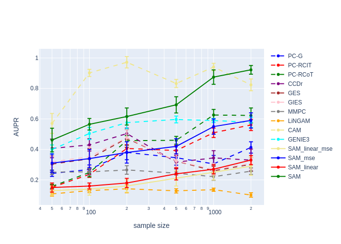
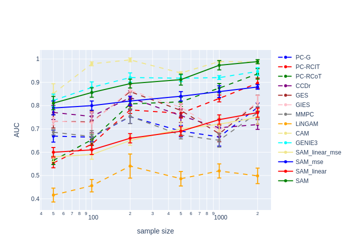


Appendix F Parametric loss : systematic experiment of Markov equivalence class disambiguation
Let us consider synthetic graphs where each variable has a single parent. In this graphs there are no v-structures. The only way for SAM to distinguishing within the same Markov equivalence is to use the parametric loss. We consider 10 synthetic graphs with 20 variables generated with the different causal mechanisms presented in section 5.1 and we compare SAM with causal pairwise methods able to disambiguate Markov equivalent DAG:
For all methods we provide the true skeleton of the graph. It only remains to orient each edge. The performance of each algorithm is assessed by measuring the AUPR and AUC scores of this binary decision task. The results obtained by the different methods are displayed on Table 17 and 18. Unsurprisingly, no method can orient the edges of Gaussian linear datasets as the pairs are completely symmetrical. It explains why the scores provided by the various methods in section 6.4 on synthetic datasets generated with linear mechanisms are in general lower than those generated with more complex mechanisms.
We also observe in Table 17 and 18 that the ANM method obtains the best scores for the datasets generated with additive noise (GP AM and Sigmoid AM) as the ANM algorithm is specifically designed to identify the causal direction when the noise is additive. Moreover the results are almost perfect for the GP AM dataset generated with Gaussian process and additive noise as it corresponds perfectly to the setting of the ANM method used here (Gaussian process regression and additive noise). However this ANM method is less good for other the datasets generated with other type of noises compared to the SAM algorithm.
We observe that SAM obtains overall good results for all type of mechanisms compared to the other pairwise methods in the task of disambiguating Markov equivalence classes.
| AUPR | Linear | GP AM | GP Mix | Sigmoid AM | Sigmoid Mix | NN | Global |
|---|---|---|---|---|---|---|---|
| IGCI | 0.58 (0.09) | 0.61 (0.05) | 0.79 (0.09) | 0.82 (0.03) | 0.58 (0.01) | 0.57 (0.04) | 0.66 (0.12) |
| ANM | 0.53 (0.06) | 0.99 (0.01) | 0.78 (0.04) | 0.83 (0.04) | 0.52 (0.07) | 0.72 (0.08) | 0.73 (0.17) |
| RECI | 0.57 (0.07) | 0.52 (0.05) | 0.51 (0.04) | 0.47 (0.01) | 0.60 (0.01) | 0.53 (0.10) | 0.54 (0.07) |
| SAM-lin-mse | 0.56 (0.08) | 0.59 (0.05) | 0.62 (0.03) | 0.56 (0.03) | 0.55 (0.03) | 0.54 (0.07) | 0.57 (0.07) |
| SAM-mse | 0.56 (0.05) | 0.82 (0.06) | 0.77 (0.05) | 0.80 (0.07) | 0.72 (0.04) | 0.75 (0.06) | 0.74 (0.13) |
| SAM-lin | 0.57 (0.08) | 0.78 (0.08) | 0.75 (0.03) | 0.79 (0.05) | 0.75 (0.03) | 0.68 (0.09) | 0.72(0.12) |
| SAM | 0.57 (0.09) | 0.85 (0.09) | 0.87 (0.04) | 0.79 (0.02) | 0.98 (0.01) | 0.95 (0.04) | 0.83 (0.15) |
| AUC | Linear | GP AM | GP Mix | Sigmoid AM | Sigmoid Mix | NN | Global |
|---|---|---|---|---|---|---|---|
| IGCI | 0.54 (0.13) | 0.59 (0.048) | 0.76 (0.083) | 0.80 (0.049) | 0.61 (0.016) | 0.57 (0.077) | 0.64 (0.13) |
| ANM | 0.54 (0.073) | 0.99 (0.013) | 0.79 (0.056) | 0.82 (0.050) | 0.49 (0.087) | 0.70 (0.111) | 0.72 (0.185) |
| RECI | 0.54 (0.10) | 0.46 (0.069) | 0.48 (0.041) | 0.36 (0.05) | 0.39 (0.018) | 0.44 (0.18) | 0.45 (0.11) |
| SAM-lin-mse | 0.51 (0.11) | 0.57 (0.07) | 0.65 (0.05) | 0.58 (0.05) | 0.49 (0.02) | 0.56 (0.06) | 0.56 (0.08) |
| SAM-mse | 0.53 (0.04) | 0.79 (0.08) | 0.73 (0.07) | 0.79(0.09) | 0.81 (0.05) | 0.72 (0.07) | 0.73 (0.10) |
| SAM-lin | 0.49 (0.02) | 0.76 (0.05) | 0.69 (0.04) | 0.78 (0.07) | 0.76 (0.07) | 0.66 (0.05) | 0.69 (0.08) |
| SAM | 0.51 (0.085) | 0.85 (0.085) | 0.84 (0.048) | 0.74 (0.023) | 0.98 (0.009) | 0.95 (0.040) | 0.81 (0.17) |
Appendix G Robustness of the various methods to non-gaussian noise
Let us consider synthetic graphs with 20 variables with 500 points and generated with the mechanisms presented in section 5.1, except that the distribution of the noise variables is set to instead of . 10 DAGs are generated for each type of mechanism. All the methods presented in Section 6 are launched on these datasets.
Table 19, 20 and 21 respectively display the AUPR, AUC and SHD scores for all the methods launched with the same hyperparameters (see Section 6). In particular, in the SAM algorithm, we keep the Gaussian noise variable as input of each generator.
We observe that SAM obtain the best scores in term of AUPR, AUC and SHD for all the datasets, except for the distribution with additive noise (GP AM and Sigmoid AM). Overall, the results are comparable to those obtained with Gaussian noise and displayed in Table 3, 4 and 5, showing to some extent that the SAM algorithm can be robust to a change in the noise distribution.
However, we notice that SAM actually performs better for the linear dataset when the noise is uniform instead of Gaussian. Indeed when the noise is uniform instead of Gaussian, it introduces distributional asymmetries in the data generative process, which allows SAM to leverage on the parametric fitting loss to orient edges in the Markov equivalence class of the DAG.
| AUPR | Linear | GP AM | GP Mix | Sigmoid AM | Sigmoid Mix | NN | Global |
|---|---|---|---|---|---|---|---|
| PC-Gauss | 0.25 (0.01) | 0.45 (0.04) | 0.27 (0.02) | 0.38 (0.03) | 0.27 (0.02) | 0.29 (0.05) | 0.32 (0.08) |
| PC-HSIC | 0.25 (0.02) | 0.52 (0.05) | 0.28 (0.01) | 0.43 (0.03) | 0.23 (0.03) | 0.32 (0.05) | 0.35 (0.08) |
| PC-RCOT | 0.24 (0.02) | 0.53 (0.06) | 0.28 (0.01) | 0.44 (0.04) | 0.31 (0.01) | 0.35 (0.05) | 0.36 (0.09) |
| PC-RCIT | 0.25 (0.02) | 0.50 (0.05) | 0.26 (0.02) | 0.40 (0.03) | 0.31 (0.01) | 0.33 (0.04) | 0.34 (0.10) |
| GES | 0.46 (0.04) | 0.45 (0.06) | 0.24 (0.03) | 0.48 (0.04) | 0.37 (0.02) | 0.30 (0.07) | 0.38 (0.10) |
| GIES | 0.52 (0.05) | 0.47 (0.05) | 0.25 (0.03) | 0.48 (0.05) | 0.38 (0.03) | 0.31 (0.09) | 0.40 (0.11) |
| MMHC | 0.25 (0.02) | 0.27 (0.02) | 0.21 (0.01) | 0.35 (0.01) | 0.27 (0.01) | 0.27 (0.01) | 0.27 (0.04) |
| LiNGAM | 0.41 (0.04) | 0.14 (0.02) | 0.13 (0.01) | 0.19 (0.01) | 0.11 (0.004) | 0.12 (0.02) | 0.19 (0.11) |
| CAM | 0.28 (0.02) | 0.91 (0.04) | 0.54 (0.03) | 0.37 (0.04) | 0.35 (0.04) | 0.32 (0.08) | 0.46 (0.22) |
| CCDr | 0.32 (0.03) | 0.43 (0.03) | 0.26 (0.02) | 0.46 (0.04) | 0.25 (0.02) | 0.42 (0.06) | 0.36 (0.09) |
| GENIE3 | 0.22 (0.04) | 0.48 (0.05) | 0.49 (0.04) | 0.34 (0.03) | 0.28 (0.03) | 0.36 (0.04) | 0.36 (0.11) |
| SAM-lin-mse | 0.62 (0.06) | 0.52 (0.03) | 0.32 (0.03) | 0.31 (0.02) | 0.32 (0.03) | 0.40 (0.05) | 0.42 (0.09) |
| SAM-mse | 0.59 (0.05) | 0.68 (0.04) | 0.58 (0.03) | 0.40(0.02) | 0.28 (0.01) | 0.51 (0.03) | 0.51 (0.06) |
| SAM-lin | 0.72 (0.04) | 0.51 (0.02) | 0.35 (0.02) | 0.34 (0.03) | 0.39 (0.03) | 0.42 (0.04) | 0.46 (0.07) |
| SAM | 0.68 (0.03) | 0.76 (0.05) | 0.72 (0.03) | 0.46 (0.03) | 0.67 (0.02) | 0.70 (0.09) | 0.67 (0.11) |
| AUC | Linear | GP AM | GP Mix | Sigmoid AM | Sigmoid Mix | NN | Global |
|---|---|---|---|---|---|---|---|
| PC-Gauss | 0.64 (0.01) | 0.77 (0.02) | 0.59 (0.01) | 0.75 (0.02) | 0.70 (0.02) | 0.70 (0.02) | 0.69 (0.06) |
| PC-HSIC | 0.63 (0.02) | 0.81 (0.02) | 0.66 (0.02) | 0.80 (0.02) | 0.66 (0.02) | 0.73 (0.04) | 0.72 (0.07) |
| PC-RCOT | 0.64 (0.01) | 0.83 (0.03) | 0.66 (0.02) | 0.81 (0.02) | 0.73 (0.01) | 0.75 (0.02) | 0.36 (0.11) |
| PC-RCIT | 0.64 (0.02) | 0.83 (0.03) | 0.64 (0.02) | 0.78 (0.02) | 0.71 (0.01) | 0.73 (0.03) | 0.72 (0.07) |
| GES | 0.81 (0.02) | 0.79 (0.04) | 0.67 (0.03) | 0.85 (0.02) | 0.81 (0.02) | 0.75 (0.08) | 0.78 (0.07) |
| GIES | 0.83 (0.03) | 0.80 (0.04) | 0.67 (0.02) | 0.84 (0.03) | 0.82 (0.02) | 0.75 (0.08) | 0.79 (0.07) |
| MMHC | 0.66 (0.02) | 0.75 (0.02) | 0.60 (0.01) | 0.78 (0.02) | 0.74 (0.01) | 0.72 (0.02) | 0.71 (0.06) |
| LiNGAM | 0.77 (0.02) | 0.57 (0.02) | 0.47 (0.02) | 0.46 (0.02) | 0.50 (0.02) | 0.50 (0.04) | 0.55 (0.11) |
| CAM | 0.73 (0.01) | 0.97 (0.01) | 0.88 (0.01) | 0.80 (0.02) | 0.76 (0.02) | 0.74 (0.05) | 0.81 (0.09) |
| CCDr | 0.74 (0.02) | 0.74 (0.03) | 0.64 (0.02) | 0.83 (0.02) | 0.69 (0.02) | 0.78 (0.05) | 0.74 (0.07) |
| GENIE3 | 0.69 (0.02) | 0.79 (0.02) | 0.71 (0.01) | 0.78 (0.01) | 0.68 (0.02) | 0.70 (0.02) | 0.73 (0.07) |
| SAM-lin-mse | 0.76 (0.02) | 0.73 (0.02) | 0.75 (0.03) | 0.71 (0.02) | 0.72 (0.04) | 0.69 (0.03) | 0.73 (0.06) |
| SAM-mse | 0.72 (0.02) | 0.79 (0.03) | 0.82 (0.02) | 0.82 (0.01) | 0.69 (0.03) | 0.75 (0.02) | 0.75 (0.07) |
| SAM-lin | 0.85 (0.02) | 0.73 (0.02) | 0.72 (0.03) | 0.76 (0.02) | 0.81 (0.02) | 0.73 (0.02) | 0.77 (0.06) |
| SAM | 0.91 (0.01) | 0.94 (0.01) | 0.92 (0.01) | 0.84 (0.01) | 0.91 (0.01) | 0.90 (0.03) | 0.91 (0.03) |
| AUPR | Linear | GP AM | GP Mix | Sigmoid AM | Sigmoid Mix | NN | Global |
|---|---|---|---|---|---|---|---|
| PC-Gauss | 52.1 (1.4) | 33.0 (2.2) | 57.8 (1.6) | 39.7 (1.7) | 47.0 (1.4) | 45.0 (3.6) | 45.8 (8.3) |
| PC-HSIC | 53.0 (1.6) | 30.4 (2.9) | 55.0 (0.3) | 36.7 (1.9) | 41.7 (0.4) | 43.0 (8.8) | 43.4 (10.2) |
| PC-RCOT | 55.4 (1.8) | 28.2 (2.6) | 54.4 (0.6) | 35.2 (1.3) | 42.9 (1.0) | 41.4 (4.0) | 42.9 (10.0) |
| PC-RCIT | 53.0 (1.6) | 30.4 (2.9) | 55.0 (0.3) | 36.9 (1.9) | 41.7 (0.4) | 41.2 (3.2) | 43.0 (8.9) |
| GES | 61.5 (4.5) | 45.1 (6.1) | 88.7 (4.0) | 42.9 (2.4) | 54.5 (4.5) | 78.9 (14.8) | 61.9 (18.3) |
| GIES | 61.8 (6.8) | 46.0 (7.2) | 88.6 (4.4) | 43.8 (2.6) | 55.3 (3.3) | 79.2 (14.4) | 62.4 (18.1) |
| MMHC | 50.8 (1.6) | 52.4 (2.8) | 72.4 (3.6) | 43.1 (1.6) | 53.1 (1.9) | 47.0 (2.9) | 53.1 (9.6) |
| LiNGAM | 46.7 (2.1) | 45.5 (2.1) | 68.2 (1.5) | 39.9 (0.7) | 54.6 (2.3) | 55.4 (5.3) | 51.7 (9.5) |
| CAM | 80.2 (2.6) | 21.4 (3.2) | 66.4 (2.9) | 62.2 (4.8) | 58.0 (4.1) | 67.1 (8.8) | 59.2 (18.8) |
| CCDr | 85.8 (5.1) | 30.5 (2.2) | 64.7 (2.6) | 39.3 (2.8) | 49.5 (1.6) | 44.9 (7.6) | 52.4 (18.7) |
| GENIE3 | 54.2 (2.3) | 32.5 (4.5) | 55.2 (3.9) | 37.2 (2.7) | 49.3 (1.9) | 46.5 (1.9) | 45.8 (9.2) |
| SAM-lin-mse | 40.2 (2.1) | 39.2 (2.5) | 43.4 (2.1) | 45.2 (3.1) | 51.3 (3.4) | 36.8 (2.4) | 42.7 (8.3) |
| SAM-mse | 45.3 (2.8) | 36.2 (2.5) | 40.3 (2.7) | 44.9 (2.8) | 53.1 (3.2) | 33.4 (2.2) | 42.2 (7.9) |
| SAM-lin | 36.1 (2.2) | 38.1 (2.4) | 41.1 (2.6) | 47.3 (3.0) | 42.8 (2.5) | 32.8 (1.9) | 39.7 (7.7) |
| SAM | 29.6 (1.7) | 23.9 (4.4) | 35.6 (3.9) | 42.3 (2.0) | 33.0 (4.1) | 26.6 (6.8) | 31.8 (7.3) |