Dense Limit of the Dawid-Skene Model for Crowdsourcing and Regions of Sub-optimality of Message Passing Algorithms

Abstract

Crowdsourcing is a strategy to categorize data through the contribution of many individuals. A wide range of theoretical and algorithmic contributions are based on the model of Dawid and Skene Dawid and Skene (1979). Recently it was shown in Ok et al. (2016a, b) that, in certain regimes, belief propagation is asymptotically optimal for data generated from the Dawid-Skene model. This paper is motivated by this recent progress. We analyze the dense limit of the Dawid-Skene model. It is shown that it belongs to a larger class of low-rank matrix estimation problems for which it is possible to express the asymptotic, Bayes-optimal, performance in a simple closed form. In the dense limit the mapping to a low-rank matrix estimation problem provides an approximate message passing algorithm that solves the problem algorithmically. We identify the regions where the algorithm efficiently computes the Bayes-optimal estimates. Our analysis refines the results of Ok et al. (2016a, b) about optimality of message passing algorithms by characterizing regions of parameters where these algorithms do not match the Bayes-optimal performance. We further study numerically the performance of approximate message passing, derived in the dense limit, on sparse instances and carry out experiments on a real world dataset.

I Introduction

The development of large-scale crowdsourcing platforms, such as Amazon’s MTurk, has popularized crowdsourcing as a simple approach to solve various problems that remain difficult for computers but require little effort to human workers. The overall strategy is simple: the requester poses a set of tasks that are allocated to several individuals from a pool of workers (the crowd). The workers answer according to their abilities and their will. Importantly, the set of answers is typically not unambiguous and post-processing has to be performed in order to infer the true information (typically labels) from the noisy observations (answers). With the crowds answers at hand the objective becomes to infer the true labels with as few mistakes as possible. The outcome of such a strategy strongly depends on the competences of the individuals; which makes it necessary to infer not only the true labels, but also the competences of the individuals.

A large fraction of the theoretical work on crowdsourcing focuses on the so-called Dawid-Skene (DS) model, after the authors of the seminal paper Dawid and Skene (1979). In the DS model we consider $N$ workers, each of them of a certain reliability that denotes the probability that a worker gives the correct answer, represented by $0\leq p^{0}_{i}\leq 1$ for worker $i=1,\dots,N$. Further there are $M$ tasks, each having a true label that we denote by $v^{0}_{j}\in\{\pm 1\}$ for task $j=1,\dots,M$. The worker $i$ is assigned a subset of tasks $j\in\partial i$ to which it assigns an answer $Y_{ij}\in\{\pm 1\}$. We denote $Y_{ij}=0$ if $j\notin\partial i$, that is for tasks $j$ that were not assigned to worker $i$. In the DS model labels provided by worker $i$ for task $j$ are modeled as

$$P(Y_{ij})=p^{0}_{i}\delta(Y_{ij}-v^{0}_{j})+(1-p^{0}_{i})\delta(Y_{ij}+v^{0}_{j})\,.$$ (1)

Moreover is it assumed that the $p^{0}_{i}$s are drawn independently from some probability distribution $P_{p^{0}}$.

The task allocation design (which tasks gets assigned to which worker) is in general part of the crowdsourcing problem and various strategies have been described and studied in the literature. It has been argued that designing the graph of assignments at random has practical and optimality advantages, among others it enables a sharp theoretical analysis of the problem, see e.g. Karger et al. (2011). On bipartite random regular graphs, where every worker is assigned $r$ tasks and every task is assigned to $l$ workers, the DS model has been studied in detail by Karger et al. (2011); Ok et al. (2016a).

While in general reconstructing the true labels and workers reliabilities from the observed answers $Y_{ij}$ is an NP-hard problem, the authors of Ok et al. (2016a, b) obtained a remarkable theorem stating that in certain regions of parameters belief propagation reconstructs the true labels optimally in the limit of large system sizes. The belief propagation algorithm for crowdsourcing was first suggested by Liu et al. (2012). Many other algorithms for crowdsourcing exist in the literature, but as far as we know none of them reaches optimal performance for large random instances of the DS model for a regime where the probability of error per task stays bounded away from zero.

The goal of the present paper is to carry out an asymptotic analysis of the DS model in the dense regime where each worker is assigned a constant fraction of the $M$ tasks. Otherwise we are in the same setting as Ok et al. (2016a, b), i.e. with random worker reliabilities and on random graphs. From our analysis it is possible to characterize more tightly the region of parameters for which belief propagation is optimal and for which it is not. We find cases where a first order phase transition appears in the error of reconstruction of the true labels. Such a first order phase transition is associated with a region of parameters in which belief propagation does not match the asymptotically optimal performance. Our work can thus be seen as a follow-up on Ok et al. (2016a, b) providing a refined analysis of the regions of parameters for which belief propagation is or is not asymptotically optimal.

In section II we first define a dense version of the DS model. In the dense DS model workers reliabilities are close to $1/2$ as otherwise inference becomes trivially easy. The dense DS model belongs to a class of low-rank matrix factorization problems, as studied recently by statistical physics techniques in Lesieur et al. (2015, 2017). The authors derived the approximate message passing (AMP) algorithm that efficiently computes the Bayes-optimal estimator and analyzed the Bayes-optimal performance in a closed form. One of the merits of AMP is that its asymptotic performance can be described via the so-called state evolution, as proven in Rangan and Fletcher (2012); Javanmard and Montanari (2013). The performance of the Bayes-optimal estimator was also later put on fully rigorous bases in the work of Miolane (2017) under assumptions that include the dense DS model as considered in section II. We apply the results derived in those papers and identify the region of parameters for which the associated approximate message passing algorithm is suboptimal. In section IV we then investigate numerically how the results – valid in the dense regime – transfer into the sparse regime as originally considered in Ok et al. (2016a, b). We finally carry out some experiments on a real world dataset to show that AMP reaches similar performance to competing state-of-the-art algorithms.

II Dense Limit of the Dawid-Skene Model

II.1 Definition of the dense limit

In this section the dense Dawid-Skene (dDS) model for crowdsourcing is introduced where each of the $N$ workers is assigned a constant fraction of the $M$ questions. It is shown that it can be modeled as a low-rank matrix factorization problem as studied in Deshpande and Montanari (2014); Matsushita and Tanaka (2013); Lesieur et al. (2015, 2017); Miolane (2017).

Let the probability that worker $i$ provides a correct answer, $p^{0}_{i}$, be close to $1/2$ and introduce the parameters $\nu$ and $\theta^{0}_{i}$ such that $p^{0}_{i}=(1+\sqrt{\nu/N}\,\theta^{0}_{i})/2$. The parameter $\nu$ is an overall scale parameter, while $\theta^{0}_{i}$ is the rescaled reliability of worker $i$ taken from some probability distribution $P_{\theta^{0}}$. In the dense limit the $1/\sqrt{N}$ scaling causes all the reliabilities to be close to $1/2$ which is the interesting regime because a total of $\Theta(N)$ answers is received for each question. If we had another scaling, the problem would become either trivially hard or easy in the thermodynamic limit, $N\to\infty$.

The true label of task $j$ is $v^{0}_{j}$, with $v^{0}_{j}\in\{\pm 1\}$ distributed as $P_{v^{0}}$. We denote with $Y_{ij}$ the label assigned to question $j$ by worker $i$ and assume $Y_{ij}\in\{0,\pm 1\}$. If $Y_{ij}=0$ question $j$ was left out by worker $i$. Set $\alpha\coloneqq\frac{M}{N}$ and consider a system in which each worker is posed $(1-\rho)M$ questions in the limit where $M,N\to\infty$, while $\alpha=\Theta(1)$ and $\rho=\Theta(1)$. In this limit the likelihood in the DS model becomes

$$\begin{split}P\left(Y_{ij}=\pm 1\mid\theta_{i},\ v_{j}\right)&=(1-\rho)\cdot\frac{1}{2}\cdot\left(1\pm\sqrt{\frac{\nu}{N}}\,\theta_{i}v_{j}\right)\\ P\left(Y_{ij}=0\mid\theta_{i},\ v_{j}\right)&=\rho\end{split}\,,$$ (2)

where we assumed that the fraction of un-answered questions, $\rho$, is independent of $(i,j)$. The rest of the present section is set in the limit where $N\to\infty$ and all the other parameters $\theta_{i},\nu,\alpha,\rho=\Theta(1)$. Later, in section IV, we will discuss how to extrapolate the results into the sparse regime where each worker is only assigned to $O(1)$ tasks.

Worker with $\theta_{i}=0$ give answers that are completely uninformative and will be called spammers. On the contrary, if $\theta_{i}\gg 1$ the answers are “strongly” aligned with the truth and we refer to such workers as hammers. Adversaries are characterized by $\theta_{i}<0$. They are also considered hammers if $\theta_{i}\ll-1$ because their answers are aligned against the truth, as opposed to the random alignment of the spammers.

II.2 Equivalence to low-rank matrix estimation

The dDS model is a special case of bipartite low-rank (rank one in the present case) matrix factorization as formulated in a much more general setting in Lesieur et al. (2017). In the rest of this section we follow closely that paper and review the results that will be applied to the present model.

In the theoretical part of this work (i.e. in all but section IV.3) we assume that the distributions from which the ground truth reliabilities $\theta_{i}^{0}$ and labels $v^{0}_{j}$ are drawn, $P_{\theta^{0}}$ and $P_{v^{0}}$ respectively, are known. Under these assumptions we aim to (a) compute efficiently the Bayes-optimal estimators of $\theta_{i}^{0}$ and $v^{0}_{j}$, given the answers $Y_{ij}$ and (b) to evaluate the asymptotic inference performance.

Denoting by $\boldsymbol{\theta}\in{\mathbb{R}}^{N}$ the vector of rescaled reliabilities for all $N$ workers, and $\mathbf{v}\in{\mathbb{R}}^{M}$ the vector of labels, we set

$$\mathbf{w}\coloneqq\frac{\boldsymbol{\theta}\,\mathbf{v}^{T}}{\sqrt{N}}$$ (3)

and re-express (2) as

$$P\left(Y_{ij}\mid w_{ij}\right)=\exp\left(g(Y_{ij},w_{ij})\right)\hskip 14.22636pt,\hskip 14.22636ptg(Y_{ij},w_{ij})=\begin{cases}\log\left(\frac{(1-\rho)}{2}\right)+\log\left(1\pm\sqrt{\nu}w_{ij}\right)&\textrm{if }Y_{ij}=\pm 1\\ \log\left(\rho\right)&\textrm{if }Y_{ij}=0\end{cases}\,.$$ (4)

From Bayes’ theorem we obtain the corresponding posterior probability distribution

$$P(\boldsymbol{\theta},\mathbf{v}\mid\mathbf{Y})=\frac{1}{Z(\mathbf{Y})}\prod_{1\leq i\leq N}P_{\theta}(\theta_{i})\prod_{1\leq j\leq M}P_{v}(v_{j})\prod_{1\leq i\leq N,1\leq j\leq M}\textrm{e}^{g(Y_{ij},w_{ij})}\,.$$ (5)

The Bayes-optimal estimates, $\hat{\boldsymbol{\theta}}$, that minimize the mean-squared-error (MSE) on $\boldsymbol{\theta}$

$$\text{MSE}_{\theta}=\frac{1}{N}\sum_{i}\left(\hat{\theta}_{i}-\theta^{0}_{i}\right)^{2}$$ (6)

and the bitwise error-rate (ER) on $\mathbf{v}$

$$\text{ER}_{v}=\frac{1}{M}\sum_{j}\mathbb{I}\left[\hat{v}_{j}\neq v^{0}_{j}\right]=\frac{1}{M}\sum_{j}\left(\frac{\hat{v}_{j}-v^{0}_{j}}{2}\right)^{2}=\frac{1}{2}\frac{1}{M}\sum_{j}\left(1-\hat{v}_{j}v^{0}_{j}\right)$$ (7)

read

$$\hat{\theta}^{\text{MMSE}}_{i}(\mathbf{Y})=\int\textrm{d}\theta_{i}\theta_{i}P\left(\theta_{i}\mid\mathbf{Y}\right)\hskip 14.22636pt\text{and}\hskip 14.22636pt\hat{v}^{\text{MER}}_{j}(\mathbf{Y})=\text{sign}\int\textrm{d}v_{j}v_{j}P\left(v_{j}\mid\mathbf{Y}\right)\,,$$ (8)

where $P\left(x_{k}\mid\mathbf{Y}\right)$, with $x_{k}\in\{\{\theta\}_{i=1,\dots,N},\{v_{j}\}_{j=1,\dots,M}\}$, is the posterior marginal of $(\ref{eq:posterior})$ after integrating out all variables except $x_{k}$. Hence inferring the reliabilities and labels in the crowdsourcing problem reduces to evaluating the marginal expectations of the posterior probability distribution. In general this is a difficult task. The contribution of the present work is to realize that the dDS model falls into a class of low-rank matrix estimation problems for which the posterior probability distribution can be evaluated, as shown in Lesieur et al. (2017). Using these results, the phase diagram can be evaluated in great detail.

II.3 Approximate message passing

The approximate message passing (AMP) algorithm for low-rank matrix estimation is a simplification of belief propagation in the limit of dense graphical models. In this limit both, belief propagation and AMP have the same asymptotic performance. However, AMP is much simpler to implement and has a favorable scaling w.r.t the problem size. It is closely related to the Thouless-Anderson-Palmer equations Thouless et al. (1977) from the theory of spin glasses, with correct time indices Bolthausen (2014); Zdeborová and Krzakala (2016). AMP for low-rank matrix factorization was first derived for special cases in Rangan and Fletcher (2012); Matsushita and Tanaka (2013) and in its general form in Lesieur et al. (2015, 2017).

AMP can be derived starting from belief propagation for the graphical model where both the reliabilities and labels are variable nodes, and there are pair-wise factor nodes corresponding to the answers $Y_{ij}$. The following two simplifications of BP are then made. First, the BP messages are replaced by their means and variances which eradicates the necessity of tracking a whole function for each message. Secondly, each (mean and variance) message is replaces by its marginal version, reducing the complexity from $O(N^{2})$ messages to $O(N)$ marginals. For details we refer the reader to Lesieur et al. (2017).

To state the AMP algorithm for the dense DS model it is necessary to specify the denoising functions $f_{\theta}(A_{\theta},B_{\theta})$ and $f_{v}(A_{v},B_{v})$ that depend on the priors $P_{\theta}$ and $P_{v}$ respectively. $A$ and $B$ are estimates for the parameters of a Gaussian distribution that are computed self-consistently. The estimate $\hat{x}_{k}$ – with $x_{k}\in\{\{\theta_{i}\}_{i=1,\dots,N},\{v_{j}\}_{j=1,\dots,M}\}$ – are then computed as the mean of the prior weighted with this effective Gaussian. The estimates for their variance are obtained from the derivative w.r.t. $B$.

$$\hat{x}\coloneqq f_{x}(A_{x},B_{x})=\frac{1}{Z_{x}(A_{x},B_{x})}\int\textrm{d}x\,x\,P_{x}(x)\,\textrm{e}^{-\frac{1}{2}A_{x}x^{2}+B_{x}x}\ ,\hskip 28.45274pt\sigma_{x}=\partial_{B_{x}}\,f_{x}(A_{x},B_{x})\,,$$ (9)

where $x$ can stay either for $\theta$ or $v$.

To state AMP we need to define the Fisher score matrix

$$S_{ij} \coloneqq \left.\frac{\partial g(Y_{ij},w_{ij})}{\partial w_{ij}}\right|_{w_{ij}=0}=Y_{ij}\cdot\sqrt{\nu}\,,$$ (10)

where $g(Y_{ij},w_{ij})$ is defined in eq. (4). Further we define the Fisher information (inverse effective noise) of the noisy observation channel

$$\Delta^{-1}=\mathbb{E}_{P(Y_{ij}\mid w_{ij}=0)}\left[\left(\left.\frac{\partial g(Y_{ij},w_{ij})}{\partial w_{ij}}\right|_{w_{ij}=0}\right)^{2}\right]=(1-\rho)\nu\,.$$ (11)

Given these definitions AMP is an iterative scheme that we outline in Algorithm 1. The numerical implementation might profit from an adequate damping scheme in order to enhance convergence even on small instances or when the model assumptions are not satisfied.

Data: $\mathbf{S},\ \Delta,\ \delta$ ;

  // $\mathbf{S}$ and $\Delta$ according to (10) and (11) respectively.

Result: MMSE estimates $\hat{\mathbf{v}}$ and $\hat{\boldsymbol{\theta}}$

Initialize: $\hat{\mathbf{v}}\leftarrow\hat{\mathbf{v}}^{\textrm{init}}\sim P_{v}(\mathbf{v})$, $\hat{\boldsymbol{\theta}}\leftarrow\hat{\boldsymbol{\theta}}^{\textrm{init}}\sim P_{\theta}(\boldsymbol{\theta})$ ; $\sigma_{v}\leftarrow 1$, $\sigma_{\theta}\leftarrow 1$; $\hat{\mathbf{v}}^{\textrm{old}}\leftarrow\mathbf{0}$, $\hat{\boldsymbol{\theta}}^{\textrm{old}}\leftarrow\mathbf{0}$ ;

while  $\lVert\hat{\boldsymbol{\theta}}-\hat{\boldsymbol{\theta}}^{\textrm{old}}\rVert_{2}^{2}+\lVert\hat{\mathbf{v}}-\hat{\mathbf{v}}^{\textrm{old}}\rVert_{2}^{2}>\delta$ do

     

     $\mathbf{B}_{\theta}\leftarrow\frac{1}{\sqrt{N}}\,\mathbf{S}\hat{\mathbf{v}}-\frac{1}{\Delta}\,\hat{\boldsymbol{\theta}}^{\textrm{old}}\sigma_{v}$ ;

     

     $\mathbf{A}_{\theta}\leftarrow\frac{1}{N\Delta}\,\hat{\mathbf{v}}^{T}\hat{\mathbf{v}}$ ;

     

     $\mathbf{B}_{v}\leftarrow\frac{1}{\sqrt{N}}\,\mathbf{S}^{T}\hat{\boldsymbol{\theta}}-\frac{\alpha}{\Delta}\,\hat{\mathbf{v}}^{\textrm{old}}\sigma_{\theta}$ ;

     

     $\mathbf{A}_{v}\leftarrow\frac{1}{N\Delta}\,\hat{\boldsymbol{\theta}}^{T}\hat{\boldsymbol{\theta}}$ ;

     

     $\hat{\boldsymbol{\theta}}^{\textrm{old}}\leftarrow\hat{\boldsymbol{\theta}}$, $\hat{\mathbf{v}}^{\textrm{old}}\leftarrow\hat{\mathbf{v}}$ ;

     

     $\hat{\boldsymbol{\theta}}\leftarrow f_{\theta}(\mathbf{A}_{\theta},\mathbf{B}_{\theta})$, $\sigma_{\theta}\leftarrow\frac{1}{N}\sum_{1\leq i\leq N}\partial_{B_{\theta_{i}}}\,f_{\theta}(A_{\theta_{i}},B_{\theta_{i}})$ ;

     

     $\hat{\mathbf{v}}\leftarrow f_{v}(\mathbf{A}_{v},\mathbf{B}_{v})$, $\sigma_{v}\leftarrow\frac{1}{M}\sum_{1\leq j\leq M}\partial_{B_{v_{j}}}\,f_{v}(A_{v_{j}},B_{v_{j}})$ ;

     

      end while

     

Algorithm 1 Approximate message passing for crowd sourcing.

II.4 State Evolution

The AMP algorithm depends on the realization of the disorder $\mathbf{Y}$ and consequently so do the AMP estimates $\hat{\boldsymbol{\theta}},\ \hat{\mathbf{v}}$ for the reliabilities and task labels. Quite remarkably, in the large size limit $N\to\infty$, the performance of the algorithm can be tracked with high probability by the so-called state evolution (SE) equations. This has been proven rigorously in Rangan and Fletcher (2012); Javanmard and Montanari (2013).

In the Bayes-optimal setting, where the true distributions $P_{\theta^{0}}$ and $P_{v^{0}}$ are known and equal to $P_{\theta}$ and $P_{v}$ respectively, the overlap of the AMP estimates with the true solution can be quantified in terms of the two order parameters

$$\begin{split}M^{t}_{\theta}&=\frac{1}{N}\sum_{1\leq i\leq N}\hat{\theta}^{t}_{i}\,\theta^{0}_{i}\,,\\ M^{t}_{v}&=\frac{1}{M}\sum_{1\leq j\leq M}\hat{v}^{t}_{j}\,v^{0}_{j}\,.\end{split}$$ (12)

Where $x^{0}$ indicates the true value of $x$, and $t$ the iteration step of the AMP equations (Alg. 1).

The SE equations imply that these order parameters evolve with high probability as

$$\begin{split}M_{v}^{t+1}&=\mathbb{E}_{v^{0},W}\left[f_{v}\left(\frac{M_{\theta}^{t}}{\Delta}\,,\,\frac{M_{\theta}^{t}}{\Delta}\,v^{0}+\sqrt{\frac{M_{\theta}^{t}}{\Delta}}\,W\right)\,v^{0}\right]\,,\\ M_{\theta}^{t}&=\mathbb{E}_{\theta^{0},W}\left[f_{\theta}\left(\frac{\alpha\,M_{v}^{t}}{\Delta}\,,\,\frac{\alpha\,M_{v}^{t}}{\Delta}\,\theta^{0}+\sqrt{\frac{\alpha\,M_{v}^{t}}{\Delta}}\,W\right)\,\theta^{0}\right]\,.\end{split}$$ (13)

where $W$ is an effective Gaussian random variable of zero mean and unit variance, $v^{0}\sim P_{v}$, $\theta^{0}\sim P_{\theta}$, the functions $f_{v}$ and $f_{\theta}$ are defined in (9), $\alpha=M/N$ and $\Delta$ is the effective noise (11).

Let us call $M^{\rm SE}_{\theta}$ and $M^{\rm SE}_{v}$ the fixed points of the SE equations (13). These fixed points are then associated to the MSE (6) and ER (7) as reached by the AMP algorithm through

$$\text{MSE}^{\rm AMP}_{\theta} = {\mathbb{E}}_{\theta}(\theta^{2})-M^{\rm SE}_{\theta}\,,$$ (14)

$$\text{ER}^{\rm AMP}_{v} = (1-R^{\rm SE}_{v})/2\,,$$ (15)

where we introduced the order parameter $R^{t}_{v}=1/M\sum_{i}\text{sign}(\hat{v}^{t}_{i})\,v^{0}_{i}$

$$R^{\rm SE}_{v}=\mathbb{E}_{v^{0},W}\left\{\text{sign}\left[f_{v}\left(\frac{M^{\rm SE}_{\theta}}{\Delta}\,,\,\frac{M^{\rm SE}_{\theta}}{\Delta}\,v^{0}+\sqrt{\frac{M^{\rm SE}_{\theta}}{\Delta}}\,W\right)\right]\,v^{0}\right\}\,.$$ (16)

II.5 Bayes-optimal error and sub-optimality of message passing algorithms

As conjectured in Lesieur et al. (2017) and proven rigorously in Miolane (2017) the performance of the Bayes-optimal estimator (8) can be evaluated in the large size limit $N\to\infty$ with $\alpha=\Theta(1)$ from the global minimizer of the so-called replica symmetric Bethe free energy, which reads

$$\phi_{\textrm{Bethe}}(M_{\theta},M_{v}) = \alpha\frac{M_{\theta}M_{v}}{2\Delta}-\alpha\mathbb{E}_{v^{0},W}\left[\log Z_{v}\left(\frac{M_{\theta}}{\Delta}\,,\,\frac{M_{\theta}}{\Delta}\,v^{0}+\sqrt{\frac{M_{\theta}}{\Delta}}\,W\right)\right]-$$ (17)

$$-\,\mathbb{E}_{\theta^{0},W}\left[\log Z_{\theta}\left(\frac{\alpha\,M_{v}}{\Delta}\,,\,\frac{\alpha\,M_{v}}{\Delta}\,\theta^{0}+\sqrt{\frac{\alpha\,M_{v}}{\Delta}}\,W\right)\right]\,.$$

where the functions $Z_{\theta}$ and $Z_{v}$ are defined in (9) and the rest of the variables are defined in the same way as in the SE. Assume $M^{*}_{\theta}$ and $M^{*}_{v}$ are the global minimizers of the above Bethe free energy. Then the minimum-mean-squared-error (MMSE) and the minimum-error-rate (MER) are expressed as

$$\text{MMSE}_{\theta} = {\mathbb{E}}_{\theta}(\theta^{2})-M^{*}_{\theta}\,,$$ (18)

$$\text{MER}_{v} = \frac{1}{2}(1-R^{*}_{v})\,,$$ (19)

where $R^{*}_{v}$ is obtained from $M^{*}_{\theta}$ via (16).

It is straightforward to observe that the SE equations are in fact stationarity conditions of the Bethe free energy. Hence the fixed points of the state evolution are critical points of the Bethe free energy. Whether or not the SE reaches the global minimizer $M^{*}_{\theta},\ M^{*}_{v}$ depends on the shape of the Bethe free energy and the initialization of the SE equations at $t=0$. Canonically the SE is initialized in such a way that the initial estimators are simply taken from the prior distributions.

We can now explain the key point of the present paper. Previous work Ok et al. (2016a, b) proved asymptotic optimality of belief propagation under certain assumptions on the parameters of the model. The present analysis of the dDS model is able to determine sharply in what regions of parameters AMP matches the Bayes-optimal estimator and when it does not, thus refining the previous picture in the limit, where AMP and BP are asymptotically equivalent.

Previously we reduced the high-dimensional model into the investigation of the two-variable free energy function (17). In particular, the phases in which AMP does not match the Bayes-optimal estimator can be characterized in terms of the critical points of the free energy and whether or not the state evolution (13) converges to the global minimum of the free energy (17). The way we check this in practice is that we initialize the state evolution in two different ways:

• Uninformative initialization, where $M_{v}^{t=0}=(\mathbb{E}_{v}(v))^{2}$ and $M_{\theta}^{t=0}=(\mathbb{E}_{\theta}(\theta))^{2}$. This corresponds to the uninformative initialization of the algorithm where the initial values of the estimators are simply taken equal to the mean of the prior distributions $P_{\theta}$ and $P_{v}$. The error achieved by the AMP algorithm is then given by iteration of (13) from this uninformative initialization.

• Informative initialization, where $M_{v}^{t=0}=\mathbb{E}_{v}(v^{2})$ and $M_{\theta}^{t=0}=\mathbb{E}_{\theta}(\theta^{2})$ so that the initial mean-squared-errors are zero. This is not possible within the algorithm without the knowledge of the ground truth and it is purely used for the purpose of the analysis. If the iteration of the SE equations (13) from this informative initialization leads to a different fixed point than from the uninformative initialization, then the free energies of the two fixed points need to be compared and the larger one surely does not correspond to the Bayes-optimal performance.

This procedure is sufficient provided there are no other fixed points. If there are, the free energy of all of them needs to be compared.

Zero-mean priors and uninformative fixed point

If both prior distributions $P_{\theta}$ and $P_{v}$ have zero mean, the uninformative initialization $M_{\theta}=M_{v}=0$ is a fixed point of the SE and equations (13) can be expanded around this fixed point. In first order we obtain

$$M_{\theta}^{t}=\frac{\alpha}{\Delta}\left(\mathbb{E}_{\theta}\left[\theta^{2}\right]\right)^{2}M_{v}^{t}$$ (20)

$$M_{v}^{t+1}=\frac{1}{\Delta}\left(\mathbb{E}_{v}\left[v^{2}\right]\right)^{2}M_{\theta}^{t}\,,$$ (21)

implying that the uninformative fixed point is numerically stable for $\Delta^{2}>\alpha\left(\mathbb{E}_{v}\left[v^{2}\right]\right)^{2}\left(\mathbb{E}_{\theta}\left[\theta^{2}\right]\right)^{2}$ and unstable otherwise. Therefore we define the critical effective noise, $\Delta_{\text{c}}$, as

$$\Delta_{\text{c}}=\sqrt{\alpha}\cdot\mathbb{E}_{\theta}\left[\theta^{2}\right]\mathbb{E}_{v}\left[v^{2}\right]\,.$$ (22)

For $\Delta<\Delta_{\text{c}}$ the uninformative initialization becomes numerically unstable. The threshold $\Delta_{\text{c}}$ correspond to the 2nd order phase transition in the behaviour of the AMP algorithm, meaning that the overlap reached by the algorithm is non-analytic and continuous at $\Delta_{\text{c}}$.

In the case where both the priors, $P_{\theta}$ and $P_{v}$, have zero mean, we can divide the region of parameters into the following three phases:

• Easy phase: The free energy (17) has a unique minimum and this minimum is associated with a positive overlap with the ground-truth configuration. Consequently iterating the state evolution (13) yields an informative fixed point from both, the informative, as well as the (perturbed) uninformative initializations. AMP is Bayes-optimal.

• Hard phase: In this phase at least two minima of the free energy (17) coexist; at least one local minimum of small overlap and a global minimum of larger overlap. The outcome of iterating the state evolution equations now depends on the initialization: while the informative initialization yields a fixed point with large overlap, the uninformative initialization leads to a fixed point of low overlap. This is precisely the region of parameters where the approximate message passing algorithms do not reach the information-theoretically optimal performance and AMP is not Bayes-optimal.

• Impossible phase: When the global minimum of (17) is associated to the trivial, non-informative, fixed point corresponding to zero overlap, we talk about a phase of impossible inference. Otherwise this region is indeed similar to the easy phase in the sense that AMP is Bayes-optimal.

If at least one of the priors has non-zero mean, then the distinction of an impossible phase is not meaningful and one would only have an easy and a hard phase, the later is defined by asymptotic sub-optimality of the AMP algorithm.

Let us further define the following three thresholds that are associated with the existence of a hard phase. The hard phase is always linked to the presence of a first order phase transition, i.e. a discontinuity in the asymptotic value of the overlap reached by the Bayes-optimal estimator. The algorithmic threshold $\Delta_{\rm alg}$ is the largest value of effective noise, $\Delta$, below which the AMP algorithm asymptotically matches the Bayes-optimal performance. The spinodal threshold, $\Delta_{\rm sp}$, is the smallest values of effective noise above which the informative initialization converges to a different fixed point than the (perturbed) uninformative initialization. The information theoretic transition, $\Delta_{\rm alg}<\Delta_{\rm IT}<\Delta_{\rm sp}$, is where the value of the Bethe free energy of the fixed point reached from the uninformative initialization crosses with the free energy of the fixed point reached from the informative initialization. The discontinuity in overlap happens at $\Delta_{\rm IT}$. Remark that while in some models, such as the stochastic block model Lesieur et al. (2015), we find $\Delta_{\text{c}}=\Delta_{\rm alg}$ in general and in the present model $\Delta_{\text{c}}\neq\Delta_{\rm alg}$.

III Phase Diagrams for the dense David-Skene model

A key property of the results we described so far is that the asymptotic behaviour of the AMP algorithm and of the Bayes-optimal estimatior depend only on the priors $P_{v}$, $P_{\theta}$ and the effective noise $\Delta=1/[(1-\rho)\nu]$. In what follows concrete priors will be considered.

It is assumed that the ground truth task labels are generated from

$$P_{v}(v_{j})=(1-\beta)\delta\left(v_{j}-1\right)+\beta\delta\left(v_{j}+1\right)\,.$$ (23)

With the parameter $\beta\in[0,1]$ accounting for a bias in the dataset.

We start our discussion with worker reliabilities $\theta_{i}$ that were drawn from a skewed Rademacher-Bernoulli (RB) prior

$$P_{\theta}(\theta)=\left(1-\mu\right)\delta(\theta)+\mu\left[(1-\lambda)\delta(\theta-1)+\lambda\delta(\theta+1)\right]\,.$$ (24)

Besides its simplicity the phase diagram for this case comprises the essential features. Tuning $\mu$ from zero to one interpolates between an uninformative crowd of mere spammers and an informative crowd. The fraction of adversaries is controlled by $\lambda$. In physics terms the workers with $\theta=-1$ are spins that are coupled to the questions by an anti-ferromagnetic interaction, whereas the workers with $\theta=1$ are ferromagnetically coupled. Consequently also the adversaries enhance our ability to recover the correct labels, if they can be identified, as they align anti-parallel to the truth.

The RB prior is the dense version of what is sometimes referred to as the “spammer-hammer” model in the literature Karger et al. (2011): Workers are either spammers that provide random answers or hammers that align very strongly with (or opposed to) the truth. Here the situation is slightly different as we assume a very weak alignment of $\Theta(1/\sqrt{N})$, cf. (2). In the dDS sending $\nu\to\infty$ and thus $\Delta\to 0$ approximates the hammers. The limit $\nu\to N$ will be considered in section IV.

III.1 The case of symmetric priors

If $\lambda=1/2$ and $\beta=1/2$ both the priors $P_{v}$ and $P_{\theta}$ have zero mean and the SE equations in (13) have a trivial fixed point at $M^{*}_{v}=M^{*}_{\theta}=0$. Expansion around this fixed point yields

$$M_{v}^{t+1}=\alpha\frac{\mu^{2}}{\Delta^{2}}\cdot M_{v}^{t}-\alpha^{2}\frac{\mu^{2}}{\Delta^{2}}\left[\frac{\mu}{\Delta}+\frac{\mu^{2}}{\Delta^{2}}\right]\cdot\left(M_{v}^{t}\right)^{2}+O((M_{v}^{t})^{3})\,.$$ (25)

The linear term gives the stability criterion of the trivial fixed point that we had already derived in (22)

$$\Delta_{\textrm{c}}=\sqrt{\alpha}\cdot\mu\,.$$ (26)

In Fig. 1 we present the phase diagram for several values of $\alpha=M/N$. We plot the stability threshold $\Delta_{\text{c}}$ as well as the three phase transitions associated with the existence of the hard phase. We mark the phases where inference is algorithmically easy, hard and impossible. In particular, we find that a hard phase appears for small enough $\mu$ as depicted in the figure. Regions with small $\mu$ correspond to crowds that contain mostly spammers. For $\alpha=1$ the hard phase appears only if the vast majority of the workers are spammers. When $\alpha$ grows (shrinks) the hard region grows (shrinks) as well. In the region where the hard phase is absent (26) provides the right criterion to locate the phase transition from the easy to the impossible phase.

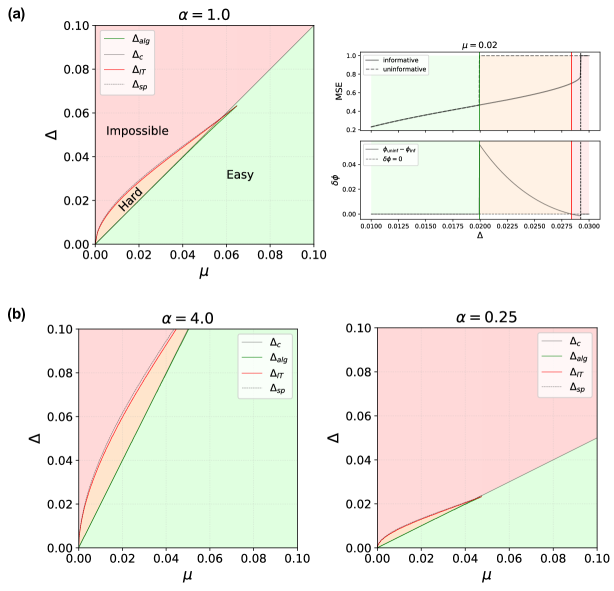
Figure 1: (a) left panel: The phase diagram for a Rademacher-Bernoulli prior on $\theta$ with $\lambda=1/2$ and no bias in the distribution of the labels ($\beta=1/2$). When the fraction of spammers is very large (small $\mu$) a hard phase appears where the AMP algorithm is not able to reach the information-theoretically optimal performance. (a) right panel: cut of the phase diagram corresponding to $\mu=0.02$, i.e. only 2% of non-spammers. We plot the MSE (top) and the difference in the free energy (bottom) of the two fixed points as a function of $\Delta$. Note that in this case we still have $\Delta_{\text{c}}>\Delta_{\rm alg}$ but both are indistinguishably close. In the hard region (orange) the AMP algorithm reaches $\text{MSE}=1$ while the Bayes-optimal estimator reaches the depicted MSE. (b) Phase diagrams with all parameters set to the same values, but $\alpha$ different. When $\alpha$ grows (shrinks) inference becomes easier (harder) and the hard region grows (shrinks). The tricritical point for $\alpha=1/4$ is located around $\mu\approx 0.048$ whereas for $\alpha=4$ it is around $\mu\approx 0.077$.

III.2 Biased labels and worker reliabilities

If $\lambda\neq 1/2$ or $\beta\neq 1/2$ the trivial fixed point $M_{v}=M_{\theta}=0$ does not exist anymore. We illustrate in Fig. 2 how this changes the phase diagram and the achievable MSE. For the case $\alpha=1$ and $\mu=0.02$ we plot the MSE reached by the state evolution from the informative and the uninformative initialization.

First (left top panel), we consider the unbiased case with $\beta=1/2$, but $\lambda\neq 1/2$ as already plotted in Fig. 1. In the bottom-left panel we consider the case where $\lambda$ changes. Due to the present symmetry it suffices to restrict the attention to $\lambda>1/2$. When more hammers than adversaries are present, i.e. for $\lambda>1/2$ the trivial fixed point at $M_{v}=0$ disappears and instead another fixed point with low but positive overlap (i.e. error smaller than 1) appears. The hard phase shrinks as shown in the bottom-left panel of Fig. 2.

If the dataset is biased, i.e. $\beta\neq 1/2$, the change is quantitatively more dramatic, but phenomenologically very similar, cf. top-right panel in Fig. 2. Upon slight change in $\beta$ the hard phase shrinks considerably. For a large range of values of $\beta$ and $\lambda$ the hard phase entirely disappears as in the bottom-right panel in Fig. 2.

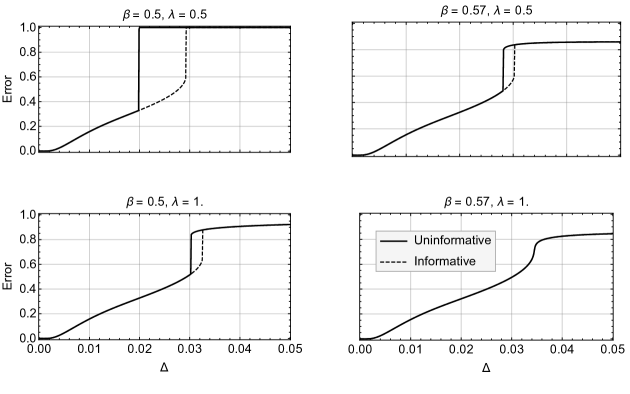
Figure 2: Influence of bias in the distribution of labels and worker reliabilities on the performance. Here we plot the resulting error rate (15) for $\alpha=1$ and $\mu=0.02$ as reached from the uninformative (bold) and informative (dashed) initialization. For bias in the labels ($\beta\neq 0.5$) or in the workers abilities ($\lambda\neq 0.5$) the trivial fixed point (error equal to one) is replaced by another fixed point with slightly lower error. The hard phase in these examples appears at larger noise and shrinks or might disappear as in the bottom right panel.

III.3 The impact of $\alpha$

Recall that $\alpha$ is the ratio of tasks to workers in our model. By virtue of the $\sqrt{\nu/N}$ scaling of the signal, cf. (2), we have two competing mechanisms when $N$ is increased: on the one hand the signal becomes weaker, on the other hand we obtain more answers per question. Equation (26) tells us that we should expect inference to become easier when $\alpha$ increases. Indeed, if we fix $\Delta$ and consider how the performance changes with $\alpha$ it follows from the SE that in order to achieve higher overlap it is necessary to increase the fraction of questions distributed to each worker, i.e. by increasing $\alpha$. This improves the estimation of $\boldsymbol{\theta}$, which in turn improves the estimate of $\mathbf{v}$. We depict this by plotting the error rate against $\alpha$ for two different values in Fig. 3.

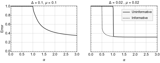
Figure 3: The behaviour of the error rate versus $\alpha$ for the RB prior (24) with $\lambda=1/2$ and bias is set to $\beta=1/2$.

How does the hard phase vary with $\alpha$? We answer this question in Fig. 1 (b) where we show that the hard phase grows further in the impossible phase when $\alpha$ is increased, while it shrinks when $\alpha$ is decreased.

III.4 Dealing with other priors

The derivation of section II applies to any prior as long as $\theta=O(1)$. Indeed, many features persist if we replace (24) by

$$P_{\theta}(\theta)=(1-\mu)\delta(\theta)+\mu\phi(\theta)\,.$$

with $\phi(\theta)$ some appropriate distribution (we have considered $\phi(\theta)$ being a beta distribution or a Gaussian). For instance (25) still holds when $\phi(\theta)$ is a standard Gaussian and as for the RB prior a first order transition is triggered by very noisy $\theta$, i.e. only very few hammers and mostly spammers in the crowd.

One might also replace the delta distribution by some other sparsity inducing distribution. A case for which the corresponding integrals are tractable analytically is that of a mixture of two Gaussians, centered around $\bar{\theta}_{L}$ ($\bar{\theta}_{R}$) with variance $\sigma_{L}^{2}$ ($\sigma_{R}^{2}$).

$$P_{\theta}(\theta)=(1-\mu)\,\mathcal{N}(\theta;\bar{\theta}_{L},\sigma_{L}^{2})+\mu\,\mathcal{N}(\theta;\bar{\theta}_{R},\sigma_{R}^{2})\,.$$

Under this choice and with $\beta=1/2$ in (23) the SE equations (13) can be expressed as

$$M_{v}^{t+1}=G\left(\frac{1}{\Delta}T\left(\frac{\alpha}{\Delta}M_{v}^{t}\right)\right)$$ (27)

with

$$G(x) =\mathbb{E}_{W}\left\{\tanh(x+\sqrt{x}W)-\tanh(-x+\sqrt{x}W)\right\}$$

$$T(q) =\mu\cdot\mathbb{E}_{W}\left\{\frac{\left[\left(\bar{\theta}_{R}+\sqrt{\frac{q}{1+q\sigma_{R}^{2}}}\sigma_{L}^{2}W\right)+\frac{1-\mu}{\mu}\left(\frac{1+q\sigma_{R}^{2}}{1+q\sigma_{L}^{2}}\right)^{\frac{3}{2}}\left(\frac{\bar{\theta}_{L}+q\sigma_{L}^{2}\bar{\theta}_{R}}{1+q\sigma_{R}^{2}}+\sqrt{\frac{q}{1+q\sigma_{R}^{2}}}W\right)\cdot\exp\left(-\frac{1}{2}Q(W)\right)\right]^{2}}{1+\frac{1-\mu}{\mu}\sqrt{\frac{1+q\sigma_{R}^{2}}{1+q\sigma_{L}^{2}}}\exp\left(-\frac{1}{2}Q(W)\right)}\right\}$$

$$Q(W) =\frac{1+q\sigma_{R}^{2}}{1+q\sigma_{L}^{2}}\left(W+\sqrt{\frac{q}{1+q\sigma_{R}^{2}}}(\bar{\theta}_{R}-\bar{\theta}_{L})\right)-W^{2}\,,$$

where $\mathbb{E}_{W}$ indicates the average over the standard Gaussian measure on $W$. Varying the means ($\bar{\theta}_{L}$, $\bar{\theta}_{R}$) and variances ($\sigma_{L}^{2}$, $\sigma_{R}^{2}$) then allows to interpolate between different scenarios.

IV Relevance of the results in the sparse regime

Our analysis of the dense DS model is based on the ground that the underlying graphical model (the bipartite question-worker-graph) is densely connected. This means that each task-node is connected to $\Theta(N)$ worker-nodes – and reversely each worker-node is connected to $\Theta(M)$ task-nodes. Allowing that some of the tasks remain unanswered introduces a sense of sparsity in the channel (cf. (2)). Our analysis assumes that $1-\rho=\Theta(1)$. Existing mathematical literature on low-rank matrix estimation shows that the formulas we derived for the Bayes-optimal performance, hold true even when the degrees in the graph grow with $N$ slower than linearly, i.e. when $(1-\rho)N$ diverges with $N\to\infty$ Deshpande et al. (2016); Caltagirone et al. (2017). The regime where the above asymptotic results do not hold anymore is when $1-\rho=O(1/N)$, which we refer to as the sparse regime. In this section we investigate numerically how the behaviour of the sparse DS model deviates from the predictions drawn from the dense DS model.

In the sparse regime considered here every worker is connected to $d$ randomly chosen tasks, where $d=\Theta(1)$. Unless the quality of each answer is very high, the effective noise $\Delta=[(1-\rho)\nu]^{-1}$ is overwhelming and inference impossible, unless $\nu=\Theta(N)$. Therefore we will consider the following “mapping”

$$\rho=1-\frac{d}{M}\hskip 28.45274pt\nu=n\cdot N\,,$$ (28)

with $n\in[0,1]$ being a constant. Consequently in the sparse regime we are dealing with high quality workers as compared to the dense regime. This brings us close to the setting of previous literature on the DS model Karger et al. (2011); Liu et al. (2012); Ok et al. (2016a, b).

IV.1 Approximate message passing on sparse graphs

We study numerically how the AMP algorithm behaves when the average degree of the nodes is small. In the following we will set $M=N$ such that the average degree of the task-nodes equals the average degree, $d$, of the worker-nodes.

Figure 4 (a) depicts results that are obtained by running AMP in the dense regime where $d=\Theta(N)$, for a system with $10^{4}$ nodes. Except from finite size effects close to the phase transition the SE prediction agrees with the empirical results. For Fig. 4 (b) we fixed different values of $\Delta$ – by adjusting $n$ so that $\Delta=\alpha/(nd)$ – and plotted the relative deviation from the SE when the degree $d$ is varied. We also show the results obtained with the BP algorithm of Liu et al. (2012) that are obtained by matching the prior and signal to noise ratio. In the limit of large $N$ the BP results are exact even for finite $d$. We find as expected that when $d$ is increased, the AMP performance approaches the prediction of the associated dense model and so does BP. While for very small $d$ BP slightly outperforms AMP, the difference is not very significant (up to fluctuations).

We further quantify the difference in performance of BP and AMP in the sparse regime in Fig. 5. Now $\nu$ (i.e. $n$) is fixed and $d$ (and hence $\Delta$) varies. We compare AMP with its BP equivalent and find that BP always outperforms AMP, but again only slightly. The general trend is as expected: in the sparse regime BP is optimal and no other algorithm can outperform it. However, it is remarkable how quickly AMP becomes comparable to BP. In Fig. 5 (b) we fix $d$ and vary $\nu$ (i.e. $n$), such that $\Delta$ varies in the same range as in Fig. 5 (a). We cannot explore the full range of $\Delta$ because we must restrict $n\leq 1$.

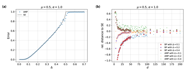
Figure 4: Evaluation of the AMP results in the sparse regime. (a) Numerical results for AMP in the dense regime for $N=M=10^{4}$, averaged over $20$ samples. (b) The relative distance of the AMP results to the SE prediction of the error when the average degree $d$ and signal to noise ratio $\nu$ are varied such that $\Delta$ remains fixed. We also compare to the BP algorithm that is asymptotically exact in the sparse regime. We see that the SE gives an accurate description, already for $d$ around $30-50$. While AMP is suboptimal for low degrees $d$ and BP still asymptotically optimal, we see that AMP and BP give comparable results down to average degrees around $10$.

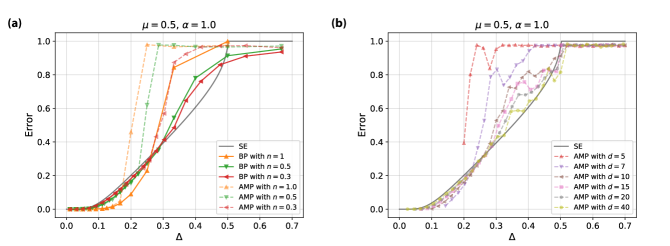
Figure 5: The effect of variation of either $d$ or $\nu$ (i.e. $n$) on the performance of AMP. (a) AMP results for fixed $\nu$. We also compared to the BP results that have the same prior and matching signal to noise ratio. (b) AMP results for fixed $d$. The fact that the error found in the experiments for large $\Delta$ is slightly below the SE is due to finite size effects. Increasing the average degree pushes the results closer to the SE prediction. The experiments were carried out with $N=10^{3}$ and are averaged over $100$ samples.

The results clearly suggests that (for finite size systems) AMP can indeed be run even on relatively sparse instances. Compared to BP it is algorithmically less complex and more memory efficient, as fewer messages need to be stored. Further, the state evolution prediction seems to remain a good qualitative approximation to the algorithmic performance. It suggests that the phenomenology found in the dense limit should be rather generic and also appear in sparse systems.

IV.2 First order phase transition in belief propagation

So far we have shown that the dense DS model can exhibit both second and first order phase transitions. The first order transitions are more interesting algorithmically as they are associated with the presence of an algorithmically hard region where the corresponding message passing algorithm is suboptimal.

The authors of Ok et al. (2016a, b) established that BP is optimal in the sparse DS model for sufficiently large signal-to-noise-ratio. It remains to be tested whether we can observe a first order phase transition also in the sparse version of the model. This shall be the aim of the present section.

Suboptimality of BP is associated with a region of parameters for which BP converges to different fixed points from the informative and from the uninformative initialization. We use our intuition based on the results of the dense case to show that there exist regimes where BP is sub-optimal. Figure 6 depicts numerical results obtained for BP with a Bernoulli-prior on $\boldsymbol{\theta}$ ($\lambda=0$ in (24)) with very sparse signals ($\mu=0.01$). We also plot the AMP performance (in the same sparse regime) as well as the asymptotic prediction that would be expected in the dense case (28). Indeed, a clear first order transition appears. This establishes the suboptimality of BP by virtue of the dependency on the initialization.

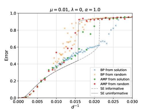
Figure 6: Numerical results obtained for the BP algorithm of references Liu et al. (2012); Ok et al. (2016a). The experiments were carried out on graphs of size $N=M=10^{4}$, and are reported as a function of the inverse average degree of the worker nodes $d$. A region of coexistence associated to a first order phase transition opens up and an informative initialization leads to another fixed point than the uninformative one. This makes BP sub-optimal in the part of this region, where the free energy of the fixed point reached from the uninformative initialization is higher than the one of the fixed point reached from the informative initialization. We found in our experiments that the first order transition appears more pronounced the larger the system size, suggesting that the phenomenon persists asymptotically.

IV.3 Approximate message passing on real data

We tested the AMP algorithm (Alg. 1) on the bluebird dataset of Welinder et al. Welinder et al. (2010). This dataset is fully connected, minimizing effects introduced by poorly designed task-worker-graphs. We used the same priors and parameters as in Liu et al. (2012) to compare AMP to other algorithms. Following Liu et al. (2012) we also implemented a “two-coin” extension of AMP that assumes that the true positive and true negative rates are different. We define $\vec{\theta}_{i}=(s_{i},t_{i})$ with $s_{i}$ the sensitivity of worker $i$ and $t_{i}$ indicating its specificity. We have

$$P\left(Y_{ij}=\pm 1\mid\vec{\theta}_{i},\ v_{j}=+1\right) =(1-\rho)\cdot\frac{1}{2}\cdot\left(1\pm\sqrt{\frac{\nu}{N}}\,s_{i}\right)$$

$$P\left(Y_{ij}=\pm 1\mid\vec{\theta}_{i},\ v_{j}=-1\right) =(1-\rho)\cdot\frac{1}{2}\cdot\left(1\mp\sqrt{\frac{\nu}{N}}\,t_{i}\right)$$

$$P\left(Y_{ij}=0\mid\vec{\theta}_{i},\ v_{j}\right) =\rho\,.$$

As in section II.2 we cast the above model into a rank-$2$ matrix factorization problem by setting

$$\vec{v_{j}}=\begin{pmatrix}1\\ 0\end{pmatrix}\ \text{if question $j$ is true}\text{ and }\vec{v_{j}}=\begin{pmatrix}0\\ -1\end{pmatrix}\ \text{if question $j$ is false}\,.$$

The only difference is that the former rank-$1$ matrix $\mathbf{w}$, cf. (3), now becomes a rank-$2$ matrix with $\boldsymbol{\theta}\in\mathbb{R}^{M\times 2}$ and $\mathbf{v}\in\mathbb{R}^{N\times 2}$. The equations for a general rank are derived and given in detail in Lesieur et al. (2017).

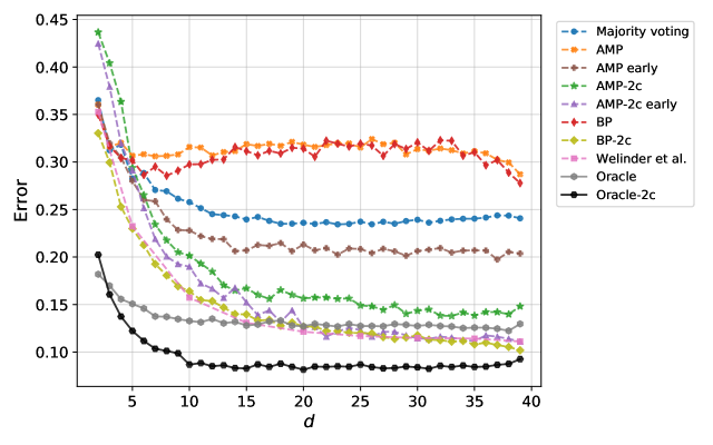
Figure 7: The error against the number of workers-per-task, $d$. Different algorithms are compared to AMP on the bluebird dataset. We compare to the results obtained with BP, majority voting and the algorithm proposed by Welinder et al. Welinder et al. (2010). As explained in the text, we implemented two different version of AMP and BP: a symmetric one in which the sensitivity and specificity are equal and an asymmetric version (referred to as “2-c” in the legend). Finally we also plot results obtained when AMP is run with an early stopping criterion of $10$ iterations. For BP and AMP the priors are set to independent $\text{Beta}(2,1)$ distributions on $\boldsymbol{\theta}$. We averaged over $100$ samples for each $d$.

In Fig. 7 we compare AMP with BP, majority voting and the algorithm developed by Welinder et al. in Welinder et al. (2010). We also compute the oracle lower bound of Karger et al. (2011) for the two versions of AMP and BP. To evaluate the oracle it we first estimate the true parameters $\boldsymbol{\theta}$ from the ground truth and then compute the resulting Bayes-optimal estimator that maximizes the posterior probability. Note that the latter estimator has full information of the workers reliabilities.

We stress that analogous comparisons between existing algorithms and BP were already performed in Liu et al. (2012), where BP was found to be superior. Our main point in this section is that AMP, which is simpler than BP, gives a comparable performance to BP even on real-world data. We therefore focus on the comparison between BP and AMP. Both, BP and AMP perform badly when the original model with $s_{i}=t_{i}$ is used as can be seen from Fig. 7 by comparing them to majority voting as a baseline algorithm. Running the same experiments with the two-coin version improves the results significantly. Indeed BP and AMP perform essentially as well as the much more involved algorithm of Welinder et al. (2010).

The experiments were run with identical beta-priors for BP and AMP ($a=2$, $b=1$) for comparability with the results in Liu et al. (2012); Ok et al. (2016b). For AMP different strategies were implemented for the prior on $\mathbf{v}$. Setting $\sigma$ to the true value (estimated from the ground truth) or to $1/2$ led to comparable results as when it was learned. In our AMP implementation we initialize $\hat{\mathbf{v}}$ in the estimates obtained by majority voting.

In the symmetric case BP and AMP are very close in performance. The difference for the two-coin models tends to be slightly larger, while the general trend persists. We also observe that it can be beneficial to implement AMP with an early stopping criterion as depicted in Fig. 7. Early stopping can be reasonable because the assumptions made in the derivation are likely to be imprecise, especially for small system sizes.

In summary, AMP performs quite well on real world datasets. The vanilla implementation yields slightly worse results, as compared to BP. However, when AMP is stopped after few iterations (we used $10$) it reaches much better performance in the rank-$1$ case. A significant improvement is also obtained in the rank-$2$ version of AMP: for small $d$ BP outperforms AMP, but they soon become quasi indistinguishable. Besides its good performance it has the great advantage of algorithmic simplicity, better time complexity and scalability.

V Conclusion

In this paper the dense limit of the Dawid-Skene model for crowdsourcing was considered. It was shown that the problem can be mapped onto a larger class of low-rank matrix factorization problems. This leads to an approximate message passing algorithm for crowdsourcing and a closed-form asymptotic analysis of its performance. Due to the previous work of Barbier et al. (2016); Miolane (2017) this analysis can be considered rigorous. While the theory only holds rigorously for the dense Dawid-Skene model, numerical experiments suggest that in the sparse regime AMP still performs well and also the asymptotic analysis provides a good qualitative prediction.

When the crowd consists mainly of spammers with only few workers that provide useful information, we found that a first order transition appears in the Bayes-optimal performance. Algorithmically this first order transition translates into the presence of a hard phase in which the AMP algorithm is sub-optimal. As a proof of concept we showed numerically that this feature persists even in the sparse regime where the rigor of our analysis breaks down. In experiments we also found instances of first order transitions in the belief propagation algorithm of Liu et al. (2012). This shows that there are regimes in the Dawid-Skene model where BP is not optimal. This complements recent results on Ok et al. (2016a, b) about regimes of optimality of BP.

We also carried out experiments on real-world data and showed that AMP performs comparable to other state-of-the-art algorithms, while being of lower time complexity. Our experiments on the real-world dataset also show that having a model that described data accurately is more important than the precise algorithm that is used to do do inference on the model.

References

- Dawid and Skene (1979) A. P. Dawid and A. M. Skene, “Maximum likelihood estimation of observer error-rates using the EM algorithm,” Journal of the Royal Statistical Society. Series C 28, 20–28 (1979).
- Ok et al. (2016a) Jungseul Ok, Sewoong Oh, Jinwoo Shin, and Yung Yi, “Optimality of belief propagation for crowdsourced classification,” in International Conference on Machine Learning (2016) pp. 535–544.
- Ok et al. (2016b) Jungseul Ok, Sewoong Oh, Jinwoo Shin, and Yung Yi, “Optimal inference in crowdsourced classification via belief propagation,” arXiv preprint arXiv:1602.03619 (2016b).
- Karger et al. (2011) David R. Karger, Sewoong Oh, and Devavrat Shah, “Iterative learning for reliable crowdsourcing systems,” in Advances in Neural Information Processing Systems 24 (2011) pp. 1953–1961.
- Liu et al. (2012) Qiang Liu, Jian Peng, and Alexander T Ihler, “Variational inference for crowdsourcing,” in Advances in Neural Information Processing Systems 25 (2012) pp. 692–700.
- Lesieur et al. (2015) Thibault Lesieur, Florent Krzakala, and Lenka Zdeborová, “MMSE of probabilistic low-rank matrix estimation: Universality with respect to the output channel,” in 53rd Annual Allerton Conference on Communication, Control, and Computing (2015) pp. 680–687.
- Lesieur et al. (2017) Thibault Lesieur, Florent Krzakala, and Lenka Zdeborová, “Constrained low-rank matrix estimation: phase transitions, approximate message passing and applications,” Journal of Statistical Mechanics: Theory and Experiment , 073403 (2017).
- Rangan and Fletcher (2012) Sundeep Rangan and Alyson K Fletcher, “Iterative estimation of constrained rank-one matrices in noise,” in IEEE International Symposium on Information Theory Proceedings (2012) pp. 1246–1250.
- Javanmard and Montanari (2013) Adel Javanmard and Andrea Montanari, “State evolution for general approximate message passing algorithms, with applications to spatial coupling,” Information and Inference 2, 115–144 (2013).
- Miolane (2017) L. Miolane, “Fundamental limits of low-rank matrix estimation: the non-symmetric case,” arXiv preprint arXiv:1702.00473 (2017).
- Deshpande and Montanari (2014) Yash Deshpande and Andrea Montanari, “Information-theoretically optimal sparse PCA,” in IEEE International Symposium on Information Theory (2014) pp. 2197–2201.
- Matsushita and Tanaka (2013) Ryosuke Matsushita and Toshiyuki Tanaka, “Low-rank matrix reconstruction and clustering via approximate message passing,” in Advances in Neural Information Processing Systems 26 (2013) pp. 917–925.
- Thouless et al. (1977) D. J. Thouless, P. W. Anderson, and R. G. Palmer, “Solution of ’Solvable model of a spin glass’,” The Philosophical Magazine: A Journal of Theoretical Experimental and Applied Physics 35, 593–601 (1977).
- Bolthausen (2014) Erwin Bolthausen, “An iterative construction of solutions of the TAP equations for the Sherrington–Kirkpatrick model,” Communications in Mathematical Physics 325, 333–366 (2014).
- Zdeborová and Krzakala (2016) Lenka Zdeborová and Florent Krzakala, “Statistical physics of inference: Thresholds and algorithms,” Advances in Physics 65, 453–552 (2016).
- Deshpande et al. (2016) Y. Deshpande, E. Abbe, and A. Montanari, “Asymptotic mutual information for the binary stochastic block model,” in IEEE International Symposium on Information Theory (2016) pp. 185–189.
- Caltagirone et al. (2017) Francesco Caltagirone, Marc Lelarge, and Léo Miolane, “Recovering asymmetric communities in the stochastic block model,” IEEE Transactions on Network Science and Engineering PP, 1–1 (2017).
- Welinder et al. (2010) Peter Welinder, Steve Branson, Pietro Perona, and Serge J. Belongie, “The multidimensional wisdom of crowds,” in Advances in Neural Information Processing Systems 23 (2010) pp. 2424–2432.
- Barbier et al. (2016) Jean Barbier, Mohamad Dia, Nicolas Macris, Florent Krzakala, Thibault Lesieur, and Lenka Zdeborová, “Mutual information for symmetric rank-one matrix estimation: A proof of the replica formula,” in Advances in Neural Information Processing Systems 29 (2016) pp. 424–432.