Low complexity algorithms in knot theory

Abstract.

We show that the genus problem for alternating knots with $n$ crossings has linear time complexity and is in Logspace$(n)$. Almost all alternating knots of given genus possess additional combinatorial structure, we call them standard. We show that the genus problem for these knots belongs to $TC^{0}$ circuit complexity class. We also show, that the equivalence problem for such knots with $n$ crossings has time complexity $n\log(n)$ and is in Logspace$(n)$ and $TC^{0}$ complexity classes.

1. Introduction

Determining whether a given knot is trivial or not is one of the central questions in topology. Dehn’s work [9] led to the formulation of the word and isomorphism problems, which played the major role in the development of the theory of algorithms. The first algorithm for the unknotting problem was given by Haken [10]. Haken s procedure is based on normal surface theory. Hass, Lagarias and Pippenger showed that Haken s unknotting algorithm runs in time at most $C^{t}$ where the knot $K$ is embedded in the 1-skeleton of a triangulated manifold $M$ with $t$ tetrahedra, and $C$ is a constant independent of $M$ and $K$, see [11]. They also showed that the unknotting problem is in NP. Agol, Haas and Thurston [1] showed that the problem of determining a bound on the genus of a knot in a 3-manifold, is NP-complete. For more details on NP and co-NP problems in knot theory see an excellent survey by Lackenby [15]. This shows that (unless P=NP) the genus problem has high computational complexity even for knots in a 3-manifold.

In this paper we initiate the study of classes of knots where the genus problem and even the equivalence problem have very low computational complexity. We show that the genus problem for alternating knots with $n$ crossings has linear time complexity and is in Logspace$(n)$. Almost all alternating knots of given genus possess additional combinatorial structure, we call them standard. We show that the genus problem for these knots belongs to $TC^{0}$ circuit complexity class. We also show, that the equivalence problem for such knots with $n$ crossings has time complexity $n\log(n)$ and is in Logspace$(n)$ and $TC^{0}$ complexity classes.

Recall, that $AC^{0}$ ($TC^{0}$ ) is the class of functions computed by constant depth boolean circuits of unbounded fan-in AND, OR, and NOT gates (MAJORITY gates, respectively). The relationship is as follows $TC^{0}\subseteq L\subseteq P$, where $P$ is the class of polynomial time problems.

The main tool applied in our algorithms are quadratic words in a free group. Such words with some additional structure are called Wicks forms. It was shown in [26] that the alternating diagrams obtained from planar maximal Wicks forms are standard alternating, and an unexpected consequence of this result is that generically an alternating knot of any genus (higher than one) is a standard alternating knot.

For basic knot theoretic definitions see [23].

2. Statement of results and structure of the paper

Seifert algorithm if a standard tool to associate an orientable surface with a boundary to a knot, which can be found in, for example [23], but we remind it here for the completeness of the arguments.

Seifert’s Algorithm(1934, Herbert Seifert):

• Input := a knot $K$.

• Output := an orientable surface $S_{k}$ with boundary component $K$.

Algorithm:

1. Start with a diagram of $K$.

2. Give it an orientation.

3. Eliminate the crossings as follows: First note that at each crossing two strands come in and two come out. Then connect each of the strands coming into the crossing to the adjacent strand leaving the crossing.

4. Fill in the circles, so each circle bounds a disk.

5. Connect the disks to one another, at the crossings of the knots, by twisted bands.

Definition 2.1.

The oriented circles appearing in the Seifert’s Algorithm are called Seifert Circles.

We note, that by changing the orientation we get the same Seifert Circles but with opposite orientation. Therefore the result is independent of the orientation.

Definition 2.2.

For a diagram $D$ of knot $K$, we define the genus $g(D)$ as the genus of the surface obtained by applying the Seifert algorithm to this diagram. It can be expressed as

$$g(D)=\frac{c(D)-s(D)+1}{2}\,,$$

with $s(D)$ being the number of Seifert circles of $D$.

Definition 2.3.

A planar diagram is alternating if the over-crossings and under-crossings alternate. A knot is alternating if it has an alternating diagram.

Theorem 2.4.

The genus problem for alternating knots with $n$ crossings has linear time complexity and is in Logspace$(n)$. For an arbitrary knot diagram there is an algorithm with the same complexity that determines the genus of the diagram. The genus problem for standard (see Definition 4.9) alternating knots with $n$ crossings is in $TC^{0}$ complexity class.

Theorem 2.5.

The isomorphism problem for standard alternating knots with $n$ crossings has time complexity $n\log(n)$ and is in Logspace$(n)$ and $TC^{0}$ complexity classes.

The paper is organized as follows: we start with some relevant definitions and known facts in Section 3, Section 4 includes explanations why almost all alternating knots are standard. Section 5 describes an algorithm of getting a standard alternating knot using a Bieulerian path in a 3-connected planar 3-valent graph. Section 6 defines extended Wicks forms. Sections 7 and 8 bring all facts together to prove the main results.

3. Preliminaries and genus problem for alternating knots

We start with some classical definitions and recall important properties of alternating knots and links.

Definition 3.1.

A crossing $p$ in a knot diagram $D$ is called reducible (or nugatory) if $D$ can be represented in the form

$D$ is called reducible if it has a reducible crossing, else it is called reduced.

Definition 3.2.

Denote by $c(D)$ the crossing number of a knot diagram $D$. The crossing number $c(K)$ of a knot $K$ is the minimal crossing number $c(D)$ of all diagrams $D$ of $K$.

Theorem 3.3.

([13, 20, 27]) An alternating knot with a reduced alternating diagram of $n$ crossings has crossing number $n$.

Definition 3.4.

For a diagram $D$ of knot $K$, we define the genus $g(D)$ as the genus of the surface obtained by applying the Seifert algorithm to this diagram. It can be expressed as

$$g(D)=\frac{c(D)-s(D)+1}{2}\,,$$

with $s(D)$ being the number of Seifert circles of $D$.

The importance of this definition relies on the following classical fact:

Theorem 3.5.

([8, 19]) An alternating knot with an alternating diagram of genus $g$ has genus $g$.

Theorems 3.3 and 3.5 imply that to determine the genus and the crossing number of an alternating knot it is sufficient to consider its alternating diagram. It has the same genus and crossing number.

Knots diagrams give rise to quadratic words in the following way.

Knots (smooth embeddings of ${\mathbb{S}}^{1}$ to ${\mathbb{R}}^{3}$) are usually presented by knot diagrams that are generic immersions of ${\mathbb{S}^{1}}$ to ${\mathbb{R}}^{2}$-plane enhanced by information of over-passes and under-passes at the double points. To correspond a quadratic word to a knot diagram $D$ one assigns a letter to each double point of the immersion, and the preimages of each double point are denoted by this letter with opposite exponents, 1 and -1.

Our algorithm of computing the genus of an alternating diagram is based on the fact that the genus of an alternating diagram and the corresponding quadratic word coincide, what is shown by the following theorem.

Theorem 3.6.

The genus of an alternating diagram is the same as the genus of the corresponding quadratic word.

Proof.

By the Theorem 3.5 the genus of an alternating knot $K$ is equal to the genus of an alternating diagram of $K$. It was shown in [25] that the genus of an alternating diagram is equal to the genus of the corresponding quadratic word. ∎

4. Introduction to standard knots

By the work of Menasco and Thistlethwaite [18], alternating knots are related to diagrammatic move called flype.

Definition 4.1.

A flype is a move on a diagram shown in figure 1.

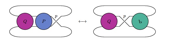
Figure 1. A flype near the crossing $p$

Theorem 4.2.

([18]) Two alternating diagrams of the same knot or link are flype-equivalent, that is, transformable into each other by a sequence of flypes.

When we want to specify the distinguished crossing $p$, we say that it is a flype near the crossing $p$.

We call the tangle $P$ of figure 1 flypable. We say that the crossing $p$ admits a flype or that the diagram admits a flype at (or near) $p$.

We call the flype non-trivial, if both tangles $P$ and $Q$ have at least two crossings.

We say that the crossing $p$ admits a (non-trivial) flype if the diagram can be represented as in figure 1 with $p$ being the distinguished crossing (and both tangles having at least two crossings). A diagram admits a (non-trivial) flype if some crossing in it admits a (non-trivial) flype.

Since trivial flypes are of no interest we will assume from now on, unless otherwise noted, that all flypes are non-trivial, without mentioning this explicitly each time.

We call the move in (1) a $\bar{t}_{2}$ move.

Theorem 4.3.

([24, theorem 3.1]) Reduced (that is, with no nugatory crossings) alternating knot diagrams of given genus decompose into finitely many equivalence classes under flypes and direct and reversed applications of $\bar{t}_{2}$ moves.

$\bar{t}_{2}$-irreducible diagram is a diagram where we cannot reduce the number of crossings using $\bar{t}_{2}$-moves.

It was observed in [24] that in a sequence of flypes and $\bar{t}_{2}$ moves, all the flypes can be performed in the beginning. It follows then from Theorems 4.2 and 4.3 that there are only finitely many alternating knots with $\bar{t}_{2}$-irreducible diagrams of given genus $g$, and we call all such knots, and their alternating diagrams generators or generating knots/diagrams of genus $g$.

A clasp is a tangle made up of two crossings. According to the orientation of the strands we distinguish between reverse and parallel clasps.

There is an obvious bijective correspondence between the crossings of the 2 diagrams in figure 1 before and after the flype, and under this correspondence we can speak of what is a specific crossing after the flype. In this sense, we make the following definition:

Definition 4.4.

We call two crossings in a diagram $\sim$-equivalent, if they can be made to form a reverse clasp after some (sequence of) flypes.

Is is an easy exercise to check that $\sim$ is an equivalence relation.

Definition 4.5.

We call an alternating diagram generating, if each $\sim$-equivalence class of its crossings has $1$ or $2$ elements. The set of diagrams which can be obtained by applying flypes and $\bar{t}_{2}$ moves on a generating diagram $D$ we call generating series of $D$.

Thus theorem 4.3 says that alternating diagrams of given genus decompose into finitely many generating series.

Definition 4.6.

Let $c_{g}$ be the maximal crossing number of a generating diagram of genus $g$, and $d_{g}$ the maximal number of $\sim$-equivalence classes of such a diagram.

Theorem 4.7.

[[26]] The following holds:

1. $d_{g,o}=d_{g,e}=6g-3$ for $g>1$. That is, $a_{n,g}\sim n^{6g-4}$.

2. $c_{g}\geq 10g-7$.

It will be convenient, from now on, to consider only genus $g>1$. The case $g=1$ is described in [24].

Definition 4.8.

We say, that an alternating knot diagram is strongly prime, if it admits the maximal number of $\sim$-equivalence classes.

Definition 4.9.

A standard diagram D of an alternating knot is a strongly prime diagram all of whose Seifert circles have either an empty interior or exterior and each of the Seifert circles of D has 2 or 3 adjacent crossings.(Here interior and exterior denote the bounded and unbounded connected component of the complement of the Seifert circle in ${\mathbb{R}}^{2}$ and empty means not containing a crossing of the knot diagram.)

Definition 4.10.

A knot admitting a standard knot diagram is called standard knot.

We consider planar 3-connected 3-valent graphs (with no multiple edges and loops). When equipping such a graph with a Bieulerian path (whenever this is possible), we associate to it a standard generating knot .

As a Bieulerian path endows each vertex of such a graph with a cyclic orientation, we have yet another appearance of, at least some, 3-valent graphs from the theory of Vassiliev invariants [4] in a different context, after Bar-Natan’s remarkable paper [3].

A consequence of such a correspondence is that standard alternating knots dominate among alternating knots of given genus (higher than 1), as the crossing number increases. The theorem below is a slight modification of results of [26], but we prove it at the end of Chapter 5 for the completeness of the paper.

Theorem 4.11.

The family of standard alternating knots is generic in the family of all alternating knots, namely the ratio of the cardinality of the set of standard alternating knots $K$ with $c(K)=n,g(K)=g,$ to the cardinality of the set of all alternating knots of the same genus and crossing number approaches 1 as $n\to\infty$ for any fixed $g>1$.

In [22] the concept of Gauß diagrams was introduced as a tool for generating knot invariants. Given a knot diagram, one links by a chord on a circle the preimages of the two passes of each crossing, orienting the chord from the underpass to the overpass. The resulting object is called a Gauß diagram (GD).

In general any circle with oriented chords is called a Gauß diagram. Not all Gauß diagrams come from knot diagrams; those that do are called realizable Gauß diagrams. We ignore in the sequel the sign of the crossings, that is, the direction of the arrows. Then realizable Gauß diagrams correspond bijectively to alternating knot diagrams up to mirroring. It was notices in [25] that the Gauß diagram of a generating diagram has no triple of chords, not intersecting each other, and intersecting the same subset of the remaining chords.

5. Standard alternating knots and 3-valent graphs

Let $G$ be a connected 3-valent graph. Fix some arbitrary orientation (direction) of the edges in $G$. A Bieulerian path in $G$ is a closed path that traverses each edge of $G$ exactly twice, only once in each direction, and does not traverse any edge followed immediately by its inverse (itself in the opposite direction).

To a Bieulerian path one can associate a word in some alphabet (called Wicks form and considered in more detail later), obtained by labeling each edge by a letter, and putting this letter (resp. its inverse) when the edge is traversed in (resp. oppositely to) its orientation.

In [25] we described the bijection between a graph with Bieulerian path $G$ and a Gauß diagram $G^{\prime}$, as the following.

To obtain $G^{\prime}$ from $G$ one just writes the letters of its word (Wicks form) $w$ along a circle and links by a chord each letter and its inverse. To obtain $G$ from $G^{\prime}$, we consider the circle of $G^{\prime}$ as a $2n$-gon (each side corresponding to a basepoint of a chord) and identify sides corresponding to the basepoints of the same chord, obtaining $G$ lying on a surface $S$. (The circle $G^{\prime}$ bounds a disk that yields $S$ under the identifications.) To indicate the origin of $G$ and $S$, we write $G=G(w)$ and $S=S(w)$. The dual of $G$ forms a 1-vertex triangulation of $S$.

We call a graph with a Bieulerian path realizable if and only if its associated Gauß diagram is realizable (as a knot diagram). In this case each Seifert circle of the knot diagram corresponds to a vertex of the graph, and each crossing of the knot diagram attached to a pair of Seifert circles corresponds to an edge joining the vertices of these Seifert circles. In this sense we call the number of crossings attached a Seifert circle its valence (the valence of its corresponding vertex in the graph).

Then in [25] we defined the genus of Gauß diagrams and of graphs in different ways and showed that they coincide. Also the genus of a knot diagram (which is equal for alternating diagrams to the genus of the knot [8, 19]) was shown to be equal to the genus of its Gauß diagram.

It is easy to see that composite knot diagrams give composite Gauß diagrams, which in turn correspond to graphs with a cut vertex. Since genus is additive under the join of graphs

as mentioned, a composite genus $g$ knot diagram can have at most $6g-6$ $\sim$-equivalence classes. Thus the contribution of such diagrams is negligible, once we have shown that there are diagrams with more $\sim$-equivalence classes (see the proof of theorem 4.7).

Definition 5.1.

A primitive Conway tangle [7] is a tangle of the form

We call two crossings $a$ and $b$ in a diagram $D$ neighbored, if they belong to a reversely oriented primitive Conway tangle in $D$, that is, there are crossings $c_{1},\dots,c_{n}$ with $a=c_{1}$ and $b=c_{n}$, such that $c_{i}$ and $c_{i+1}$ form a reverse clasp in $D$. (Equivalently, $a$ and $b$ correspond in the graph to edges which can be connected by a path passing only through vertices of valence 2.)

This is a similar definition to $\sim$-equivalence, but with no flypes allowed. Thus the number of $\sim$-equivalence classes of a diagram is not more than the number of neighbored equivalence classes of the same diagram, or of any flyped version of it.

The following was proved in [26].

Lemma 5.2.

A knot diagram of genus $g$ has at most $6g-3$ neighbored equivalence classes (and hence at most $6g-3$ $\sim$-equivalence classes).

Moreover, knot diagrams of genus $g$ having exactly $6g-3$ neighbored equivalence classes come exactly from graphs with Bieulerian path, all whose vertices have valence 2 or 3.

The lemma means in particular, that if $G^{\prime}$ is realizable and its knot diagram $D$ has $6g-3$ $\sim$-equivalence (or just neighbored equivalence) classes, then all vertices of $G^{\prime}$ have valence $2$ or $3$, and thus the Seifert circles of $D$ have $2$ or $3$ adjacent crossings. Hence the knot diagram is standard.

In general the condition of being realizable is difficult to test for $G^{\prime}$, but in the trivalent case it is surprisingly simple.

Theorem 5.3 ([26]).

A trivalent graph with Bieulerian path is realizable if and only if it is planar(ly embeddable). In this case the knot diagram is standard.

We should remark that a planar graph is in fact a graph equipped with a concrete planar embedding, while the realizability of the graph does not depend on the planar embedding. However, we will shortly show that for the cases we need to consider the planar embedding is unique (see remark 5.6).

For the proof, and later, we will need the following additional structure on a trivalent graph with Bieulerian path.

Definition 5.4.

A Bieulerian path in a trivalent graph induces an orientation on each 3-valent vertex $v$ given by a cyclic order of the 3 adjacent edges. To define it, orient the 3 adjacent edges $a$, $b$ and $c$ towards $v$. Then if the word of the Bieulerian path contains the subwords $ab^{-1}$, $bc^{-1}$ and $ca^{-1}$ (in whatever order), then the orientation at $v$ is given by $(a,b,c)$.

If the Bieulerian path contains the subwords $ac^{-1}$, $cb^{-1}$ and $ba^{-1}$ (in whatever order), then the orientation at $v$ is $(c,b,a)$.

Now we establish a natural correspondence between a planar $3$-valent graph with Bieulerian path and a standard knot diagram.

We give an explicit construction of a standard knot diagram using a planar $3$-valent graph with Bieulerian path.

Let $G$ be a 3-valent graph with Bieulerian path. The path induces the orientation of vertices. If two ends of the edge have the same orientation, put on the edge an additional vertex of degree two. We have a graph $G^{\prime}$ with vertices of degree two and three. Every edge $x$ of $G$, which was divided in two parts, will be replaced in the Bieulerian path by $x_{1}x_{2}$. We can change the orientations of the edges of $G^{\prime}$ such that in the Bieulerian path the orientations of edges alternate. Now we have an oriented graph such that for every vertex all edges incident to it either all are incoming or all are outgoing.

If all edges incident to a vertex all are outgoing (incoming) we say, that the vertex is of the first (second) type.

In the middle of any edge of $G^{\prime}$ we put a small cross, it will be a future crossing of the knot diagram. Now we draw a circle with the center in each vertex, such that the circles with centers in the ends of the same edge are tangent at the small cross. We equip each circle with the orientation induced by the orientation of the vertex. These circles will be the Seifert circles for our knot diagram.

Now we form the knot diagram from the Seifert circles by an algorithm, which is inverse to the Seifert algorithm. Overcrossings and undercrossings are defined as follows: if the knot strand goes from a vertex of the first type to a vertex of the second type, we have an overcrossing; if the strand goes from a vertex of the second type to a vertex of the first type, we have an undercrossing.

Note, that even after inserting vertices of valence 2, the graph has no edge connecting different vertices of valence 2, and thus the resulting knot diagram has not more than two neighbored crossings in each neighbored equivalence class.

Planar 3-valent graphs of genus $g$ with Bieulerian path such that the corresponding diagram has $6g-3$ $\sim$-equivalence classes are described in the following theorem.

Theorem 5.5 ([26]).

Let $G$ be a planar 3-valent graph (with Bieulerian path) and $D$ its knot diagram (as constructed earlier). Then the following conditions are equivalent:

1. $G$ is 3-connected (i.e., removing any pair of edges does not disconnect it),

2. $D$ has $6g-3$ $\sim$-equivalence classes,

3. $D$ admits no (non-trivial) flypes.

Remark 5.6.

By a theorem of Whitney each 3-valent 3-connected graph has, if any, a unique planar embedding up to moves in $S^{2}$ (see [3]). Thus for the cases that are of interest to us we do not need to care about ambiguities of the planar embedding, and can consider the graph also abstractly.

Corollary 5.7 ([26]).

There is a bijective correspondence between genus $g$ diagrams with $6g-3$ $\sim$-equivalence classes and planar 3-connected 3-valent graphs with Bieulerian paths (considered up to moves in $S^{2}$ on the graph and cyclic permutations of the path).

Proof of Theorem 4.11.

We put together the previous results. Clearly, we need to consider only genus $g$ generators $D$ of standard knots, since they have the maximal number of $\sim$-equivalence classes. By lemma 5.2, this maximal number is $6g-3$, and generators with that many $\sim$-equivalence classes have graphs with vertices of valence 2 and 3. By theorem 5.3 the diagrams of such graphs are standard, and we know from [26] that for any crossing number parity, at least one such example exists. Finally, from Part 3 of theorem 5.5 we know that diagrams in the series of D have only symmetries coming from the Bieulerian path, and the order of such a symmetry is at most 6, see [2].

6. Connection with Wicks forms

An oriented Wicks form is a cyclic word $w=w_{1}w_{2}\dots w_{2l}$ (a cyclic word is the orbit of a linear word under cyclic permutations) in some alphabet $a_{1}^{\pm 1},a_{2}^{\pm 1},\dots$ of letters $a_{1},a_{2},\dots$ and their inverses $a_{1}^{-1},a_{2}^{-1},\dots$, such that

• if $a_{i}^{\epsilon}$ appears in $w$ (for $\epsilon\in\{\pm 1\}$) then $a_{i}^{-\epsilon}$ appears exactly once in $w$,

• the word $w$ contains no cyclic factor (subword of cyclically consecutive letters in $w$) of the form $a_{i}a_{i}^{-1}$ or $a_{i}^{-1}a_{i}$ (no cancellation),

• if $a_{i}^{\epsilon}a_{j}^{\delta}$ is a cyclic factor of $w$ then $a_{j}^{-\delta}a_{i}^{-\epsilon}$ is not a cyclic factor of $w$ (substitutions of the form $a_{i}^{\epsilon}a_{j}^{\delta}\longmapsto x,\enspace a_{j}^{-\delta}a_{i}^{-\epsilon}\longmapsto x^{-1}$ are impossible).

An oriented Wicks form $w=w_{1}w_{2}\dots$ in the alphabet $A$ is isomorphic to $w^{\prime}=w^{\prime}_{1}w^{\prime}_{2}\dots$ in an alphabet $A^{\prime}$ if there exists a bijection $\varphi:A\longrightarrow A^{\prime}$ with $\varphi(a^{-1})=\varphi(a)^{-1}$ such that $w^{\prime}$ and $\varphi(w)=\varphi(w_{1})\varphi(w_{2})\dots$ define the same cyclic word.

The genus $g_{t}(w)$ of an oriented Wicks form $w=w_{1}\dots w_{2l-1}w_{2l}$ is defined as the topological genus of the oriented compact connected surface $S(w)$ obtained as described in Section 5. Knots diagrams give rise to Wicks forms in the following way.

Knots (smooth embeddings of ${\mathbb{S}}^{1}$ to ${\mathbb{R}}^{3}$) are usually presented by knot diagrams that are generic immersions of ${\mathbb{S}^{1}}$ to ${\mathbb{R}}^{2}$-plane enhanced by information of over-passes and under-passes at the double points. To correspond a Wicks form to a knot diagram $D$ one assigns a letter to each double point of the immersion, and the preimages of each double point are denoted by this letter with opposite exponents, 1 and -1.

It was shown in [25] that for alternating knots the genus of a knot and the genus of the corresponding Wicks form coniside.

Let $G$ be a cubic (3-valent) connected graph on $4g-2$ vertices and the word $U$ is one of its Bieulerian paths. We will call them cubic Wicks forms. Note that a Bieulerian path can be presented as an oriented Wicks form of genus $g$.

Definition 6.1.

Wicks forms, which came from Bieulerian paths of 3-connected planar cubic graphs on $4g-2$ vertices will be called planar Wicks forms.

These forms are also maximal in the sense of [2].

Definition 6.2.

A vertex $V$ (with oriented edges $a,b,c$ pointing toward $V$) in a cubic Wicks form $w$ is positive if

$$w=ab^{-1}\dots bc^{-1}\dots ca^{-1}\dots\quad{\rm or}\quad w=ac^{-1}\dots cb^{-1}\dots ba^{-1}\dots$$

and $V$ is negative if

$$w=ab^{-1}\dots ca^{-1}\dots bc^{-1}\dots\quad{\rm or}\quad w=ac^{-1}\dots ba^{-1}\dots ab^{-1}\dots\quad.$$

Theorem 6.3.

([2]) The number of positive vertices in a genus $g$ cubic Wicks form is $2g-2$, and the number of negative vertices is $2g$.

Definition 6.4.

Let $a$ be a letter of a Wicks form $W$. If we replace $a$ by a word $a_{1}...a_{k}$ (and its inverse by $a_{k}^{-1}...a_{1}^{-1}$), we will say that we extended the letter $a$.

Definition 6.5.

A word $V$ is an extended Wicks form, if it is obtained from a Wicks from $W$ by several extensions of letters.

7. Isomorphism problem for standard knots

From now on we consider extended Wicks forms as cyclic words, written on boundaries of discs and the graph $\Gamma$ is associated to an extended Wicks form $W$, the word $W$ is written with letters of an alphabet $\alpha$.

Theorem 7.1.

The isomorphism problem of standard genus $g$ knots with $n$ crossings given by their alternating diagrams is equivalent to the isomorphism problem of extended Wicks forms of genus $g$ and length $2n$.

Proof.

Let $K_{1}$ and $K_{2}$ be two standard knots given by their alternating diagrams. First consider the case when both $K_{1}$ and $K_{2}$ are generating diagrams. By [18] any two diagrams of alternating knots can be obtained from one another by a sequence of flypes. By the Theorem 5.5, [26], alternating diagrams of generating diagrams do not admit flypes, so the isomorphism class of a standard generating knot is uniquely determined by its alternating diagram. Alternating diagrams of $K_{1}$ and $K_{2}$ uniquely determine Gauß diagrams $D_{1}$ and $D_{2}$, and Gauß diagrams $D_{1}$ and $D_{2}$ uniquely determine two quadratic words $W_{1}$ and $W_{2}$ (see the beginning of Chapter 4). By the Theorem 5.7 and explicit description of standard alternating knots, all the vertices of the graphs $\Gamma_{1}$ and $\Gamma_{2}$ corresponding to $W_{1}$ and $W_{2}$ have valencies two or three, so $W_{1}$ and $W_{2}$ are extended Wicks forms.

Two diagrams of a(n alternating) knot in the same generating series are transformable into each other by a flype the generating diagram, see [26], p.10-11. Since the generating diagrams we consider do not admit flypes, the isomorphism type is uniquely defined by an extended Wicks form, as before.

∎

8. Computational complexity

In this section we will construct low complexity algorithms to solve some problems about strictly quadratic words in a free group and then use these algorithms to prove Theorems 2.4 and 2.5.

Proposition 8.1.

There exists an algorithm with time complexity $n\log n$ that given two strictly quadratic cyclically reduced words $w$, $w_{1}$ of length $2n$ in the free group $F(X)$ determines if there is a permutation $\sigma$ of the letters in $X$ such that $w_{1}(\sigma X)$ is a cyclic permutation of $w(X)$.

Proof.

The word $w$ of length $2n$ will be represented as an array (a string of pairs) $\mathcal{W}$ such that $W_{m}$ is a pair consisting of a letter in position $m$ of $w$ (say, $a_{m}$ or $a_{m}^{-1}=A_{m}$) and number $m$. The second array $\mathcal{V}$ consists of $n$ triples indexed by $n$ letters $a_{i}$. A triple $V_{a_{i}}$ consists of $a_{i},$ position $m$ (in binary) of $a_{i}$ and position $k$ (in binary) of $A_{i}$.

The algorithm scans the array $\mathcal{W}$ and creates the array $\mathcal{V}$. Scanning the pair $(a_{i},m)$ or $(A_{i},m)$ it puts $m$ in the second position of $V_{a_{i}}$ if this position has not been filled in yet, or in the third position if the second position has already been filled. For each triple $(a_{i},m,k)$ we compute $d_{m}=k-m$ and $d_{k}=k+2n-m$. We construct a sequence $d_{1}(w),\ldots,d_{2n}(w)$. Since we need $\mathcal{O}(\log n)$ time to subtract two numbers that are less or equal to $2n$, this takes time $\mathcal{O}(n\log n).$

Now $w_{1}(\sigma X)$ is a cyclic permutation of the word $w(X)$ if and only if the sequence $d_{1}(w_{1}),\ldots,d_{2n}(w_{1})$ is a cyclic permutation of $d_{1}(w),\ldots,d_{2n}(w)$. This can be decided in linear time in $n$ using Knuth-Morris-Pratt substring searching algorithm [14], [16]. This algorithm searches for occurrences of a word within a text string by employing the observation that when a mismatch occurs, the word itself contains sufficient information to determine where the next match could begin, thus bypassing re-examination of previously matched characters.

∎

Proposition 8.2.

There exists an algorithm with linear time complexity that computes the genus of a strictly quadratic cyclically reduced word of length $2n$ in the free group $F(X)$.

Proof.

Let $\mathcal{W}$ and $\mathcal{V}$ be the arrays defined in the proof of Proposition 8.1. We now define the graph $\Delta$ with vertices numbered from $0$ to $2n-1$ and edges obtained from the array $\mathcal{V}$. For each triple $V_{a_{i}}=(a_{i},m,k)$ there will be two edges $(m,k+1)$ and $(k,m+1).$ Each connected component of $\Delta$ represents one vertex of the graph $\Gamma$. Connected components can be of the form $\{i,j\}$ or $\{i,j,t\}$ or $\{i_{1}\ldots i_{k}\},k\leq 2n.$ BFS or DFS algorithms find connected components from the list of edges in time $\mathcal{O}(|E|)$, therefore in time $\mathcal{O}(n)$. Now we know the number of vertices $|V|$ of the graph $\Gamma$ and we know that it has $n$ edges. Therefore the Euler characteristic is $\kappa=|V|-n+1$ and the genus $g=\frac{1}{2}(2-\kappa).$

∎

We will recall definitions of some other complexity classes that we will consider.

Logspace (denoted L) is the class of functions computable by a deterministic Turing machine with working tape bounded logarithmically in the length of the input. There are two more tapes, the input tape, where we can only read but cannot write, and the output tape where we can write but cannot read while working.

For every $n,m\in N$ a Boolean circuit $C$ with $n$ inputs and $m$ outputs is a directed acyclic graph. It contains $n$ nodes with no incoming edges; called the input nodes and $m$ nodes with no outgoing edges, called the output nodes. All other nodes are called gates and are labeled with one of $\vee$, $\wedge$ or $\neg$ (in other words, the logical operations OR, AND, and NOT). The $\vee$, $\wedge$ nodes have fanin (i.e., number of incoming edges) of 2 and the $\neg$ nodes have fanin 1. The size of $C$, denoted by $|C|$, is the number of nodes in it. The circuit is called a Boolean formula if each node has at most one outgoing edge.

A $TC^{0}$ circuit with $n$ inputs is a boolean circuit of constant depth using NOT gates and unbounded fan-in AND, OR, and MAJORITY gates, such that the total number of gates is bounded by a polynomial function of $n$. A MAJORITY gate outputs 1 when more than half of its inputs are 1. A function $f(x)$ is $TC^{0}$ -computable (more casually, an algorithm is in $TC^{0}$) if for each $n$ there is a $TC^{0}$ circuit $F_{n}$ with n inputs which produces $f(x)$ on every input $x$ of length $n$. The composition of two $TC^{0}$ -computable functions is again $TC^{0}$ -computable. Since this definition of being computable only asserts that such a family ${F_{n}}_{n=1}^{\infty}$ of circuits exists, one normally imposes in addition a uniformity condition stating that each $F_{n}$ is constructible in some sense. We will only be concerned here with standard notion of DLOGTIME uniformity, which asserts that there is a random-access Turing machine which decides in logarithmic time whether in circuit $F_{n}$ the output of gate number $i$ is connected to the input of gate $j$, and determines the types of gates $i$ and $j$. We refer the reader to [30] for further details on $TC^{0}$. The problems Iterated Addition, Iterated Multiplication, Integer Division are all in $TC^{0}$ no matter whether inputs are given in unary or binary [30].

The relation between the classes is as follows:

$$TC^{0}\subseteq L\subseteq P,$$

where $P$ denotes the class of problems solvable in polynomial time.

Proposition 8.3.

There exists a Logspace algorithm that computes the genus of a strictly quadratic cyclically reduced word in the free group $F(X)$.

Proof.

The genus of the word $w(a_{1},\ldots a_{n})$ is the genus of the surface $S$ that one obtains when glues together edges with the same label of the polygon with boundary label $w$. The word $w$ becomes the label of the graph $\Gamma$ on the surface. We will write the word $w$ as a cyclic permutation. After multiplying this permutation by $\Pi_{i=1}^{n}(a_{i},a_{i}^{-1})$ we obtain a permutation $\pi$ such that the cycles of $\pi$ correspond to the vertices of $\Gamma$, see [31], Section 2, and, therefore, can compute the Euler characteristic and the genus of the surface $S$. The algorithm to represent the product of two permutations given by their cyclic representation also as a cyclic representation belongs to Logspace by [6], Theorem 3 (this is the problem PP2). ∎

Proposition 8.4.

There exists a $TC^{0}$ algorithm that computes the genus of a strictly quadratic cyclically reduced word $w$ in the free group $F(X)$ corresponding to the standard alternating knot.

Proof.

In this case the product of the involution $\Pi$ and the cycle $(w)$ corresponding to $w$ does not have cycles longer than $3$. We encode a word $w$ of length $2n$ as the array $\mathcal{W}$ from the proof of Proposition 8.1. The edges of the graph $\Delta$ represent the permutation $\sigma$ on $n$ elements presented pointwise, as the set of pairs $(k,m)$, such that $\sigma(k)=m$. We can sort (sorting in in $TC^{0}$) these pairs according to the order of the first component. To find the Euler characteristic we have to determine the number of cycles in the permutation $\sigma$. Since the knot is standard we know that the maximal length of a cycle is three.

Let the second level array have cells $\delta_{m,k}$, where $\delta_{m,k}$ contains the pair $(m,k)$ if it is an edge of $\Delta$ and contains zero otherwise.

In the next level array we will have a triple $(i,j,k)$ for each pair of edges $(i,j)$ and $(j,k)$ in $\Delta$, a pair $(i,j)$ for each pair $(i,j),(j,i)$ and zero for pairs $(i,j),(k,m)$ where $i,j,k,m$ are distinct. Then we divide the number of different triples by three and add the number of pairs. This is the number of connected components in $\Delta$ and number of vertices in $\Gamma$.

∎

Proposition 8.5.

There exists a $TC^{0}$ algorithm that given two strictly quadratic cyclically reduced words $w_{1}$, $w_{2}$ in the free group $F(X)$ determines if there is a permutation $\sigma$ of the letters in $X$ such that $w_{2}(\sigma X)$ is a cyclic permutation of $w(X)$. Therefore this problem is also in $L$.

Proof.

To decide if two words of length $n$ differ by a permutation of letters and a cyclic permutation we organize the binary circuit as follows. We encode both cyclic word $w_{1},w_{2}$ of length $n$ represented as a labelled cycle graph, as a set of triples of natural numbers (encoded as binaries) as above. We also take all cyclic permutations $w_{2k}$ of $w_{2}$ by adding $1$ to the first two entries of corresponding triples. For $w_{1},w_{2k}$ we define $\delta_{ij}(w_{1})$, $\delta_{ij}(w_{2k})$ as above. Then we compare $\delta_{ij}(w_{1})$ with each $\delta_{ij}(w_{2k})$ in parallel. If for some $k$ for all $i,j$ $\delta_{ij}(w_{1})=\delta_{ij}(w_{2k})$, then $w_{1}$ and $w_{2}$ differ by a permutation of letters and a cyclic permutation, otherwise they do not.

∎

Proof of Theorem 2.4

It was shown in [25] that for the alternating knots the genus of the knot and the genus of corresponding Wicks form coniside. The genus of a Wicks form is the same as the genus of the extended Wicks form. The statement of the theorem now follows from Propositions 8.2, 8.3 and 8.4.

Proof of Theorem 2.5

By Theorem 7.1, the isomorphism problem of standard genus $g$ knots with $n$ crossings given by their alternating diagrams is equivalent to the isomorphism problem of extended Wicks forms of genus $g$ and length $2n$. Therefore the statement of the theorem follows from Propositions 8.1 and 8.5.

Acknowledgment. The first author was supported by the PSC-CUNY award, jointly funded by The Professional Staff Congress and The City University of New York and by a grant 461171 from the Simons Foundation. The second author thanks Hunter College CUNY for the Peluso Professorship award for 2017-2018, when most of the work on this paper was done. We thank I. Agol, M. Lackenby, S. Vassileva and J. Macdonald for useful discussions and UC Berkeley and INI Cambridge for providing support.

References

- [1] I. Agol, J. Hass, and W. Thurston, The computational complexity of knot genus and spanning area, Trans. Amer. Math. Soc. 358 (2006), no. 9, 3821-3850.
- [2] R. Bacher and A. Vdovina, Counting 1-vertex triangulations of oriented surfaces, Discrete Mathematics 246(1-3) (2002), 13–27.
- [3] D. Bar-Natan, Lie algebras and the four color theorem, Combinatorica 17(1) (1997), 43–52.
- [4] by same author, On the Vassiliev knot invariants, Topology 34(2) (1995), 423–472.
- [5] R. Bott and C. Taubes, On the self-linking of knots, Jour. Math. Phys. 35(10) (1994), 5247–5287.
- [6] S. Cook, P. McKenzie, Problems Complete for Deterministic Logarithmic Space, J. of Algotithms, 8, 385-394 (1987).
- [7] J. H. Conway, On enumeration of knots and links, in “Computational Problems in abstract algebra” (J. Leech, ed.), 329-358. Pergamon Press, 1969.
- [8] R. Crowell, Genus of alternating link types, Ann. of Math. (2) 69 (1959), 258–275.
- [9] M. Dehn, Uber die Topologie des dreidimensional Raumes , Math. Annalen, 69 (1910), 137 168.
- [10] W. Haken, Theorie der Normalfl achen: Ein Isotopiekriterium f ur den Kreisknoten , Acta Math., 105 (1961) 245 375.
- [11] J. Hass, J. C. Lagarias and N. Pippenger, The computational complexity of Knot and Link problems , Journal of the ACM, 46 (1999) 185 211.
- [12] Handbook of Combinatorics, Vol. II (P. L. Graham, M. Grötschel and L. Lovácz, eds.), North-Holland, 1995.
- [13] L. H. Kauffman, State models and the Jones polynomial, Topology 26 (1987), 395–407.
- [14] D. Knuth, J. Morris, V. Pratt, Fast pattern matching in strings. SIAM Journal on Computing. 1977, 6 (2): 323 350.
- [15] M. Lackenby, Elementary knot theory Lectures on Geometry ,(Clay Lecture Notes), Oxford University Press, 2017.
- [16] Yu. Matiyasevich, Real-time recognition of the inclusion relation, Journal of Soviet Mathematics. 1: 64 70, 1973.
- [17] W. W. Menasco, Closed incompressible surfaces in alternating knot and link complements, Topology 23 (1) (1986), 37–44.
- [18] by same author and M. B. Thistlethwaite, The Tait flyping conjecture, Bull. Amer. Math. Soc. 25(2) (1991), 403–412.
- [19] K. Murasugi, On the genus of the alternating knot. I, II, J. Math. Soc. Japan 10 (1958), 94–105, 235–248.
- [20] by same author, Jones polynomial and classical conjectures in knot theory, Topology 26 (1987), 187–194.
- [21] T. Nakamura, Positive alternating links are positively alternating, J. Knot Theory Ramifications 9(1) (2000), 107–112.
- [22] M. Polyak and O. Viro, Gauss diagram formulas for Vassiliev invariants, Int. Math. Res. Notes 11 (1994), 445–454.
- [23] D. Rolfsen, Knots and links, Publish or Perish Inc., Mathematical Lecture Series 7 (1976), Berkeley CA.
- [24] A. Stoimenow, Knots of genus one, Proc. Amer. Math. Soc. 129(7) (2001), 2141–2156.
- [25] by same author, V. Tchernov and A. Vdovina, The canonical genus of a classical and virtual knot, Geom. Dedicata 95 (2002), 215–225.
- [26] by same author, A. Vdovina, Counting alternating knots by genus, Math.Ann.333, (2005), 1–27.
- [27] M. B. Thistlethwaite, A spanning tree expansion for the Jones polynomial, Topology 26 (1987), 297–309.
- [28] W. T. Tutte, A census of planar triangulations, Canad. J. Math. 14 (1962), 21–38.
- [29] A. A. Vdovina, Constructing Orientable Wicks Forms and Estimation of Their Number, Communications in Algebra 23(9) (1995), 3205–3222.
- [30] Heribert Vollmer. Introduction to circuit complexity. Texts in Theoretical Computer Science. An EATCS Series. Springer-Verlag, Berlin, 1999. A uniform approach.
- [31] T. Walsh, A. Lehman, Counting rooted maps by Genus, Journal of Combinatorial Theory, Series B, V. 13, Issue 3, December 1972, 192-218.