Global secondary bifurcation, symmetry breaking and period-doubling

Abstract.

In this paper we provide a criterion for global secondary bifurcation via symmetry breaking. As an application, the occurrence of period-doubling bifurcations for the Lugiato-Lefever equation is proved.

1. Introduction

The aim of this paper is to provide a sufficient condition for global secondary bifurcation via symmetry breaking for equations of the form

(1) $$F(x,\lambda)=0$$

where $x\in X$ belongs to a Banach space and $\lambda\in\mathbb{R}$ is a real parameter. Bifurcation theory is about finding solutions near a given family of trivial solutions of (1). For instance, if $F(0,\lambda)=0$ for all $\lambda\in\mathbb{R}$ then the trivial solution family is given by $\{(0,\lambda):\lambda\in\mathbb{R}\}\subset X\times\mathbb{R}$. More generally, if $\mathcal{T}\subset X\times\mathbb{R}$ is a family of solutions then $(x,\lambda)\in\mathcal{T}$ is a bifurcation point with respect to $\mathcal{T}$ if there is a sequence of solutions $(x_{n},\lambda_{n})\notin\mathcal{T}$ converging to $(x,\lambda)$. In this case one speaks of (primary) bifurcation with respect to $\mathcal{T}$ and there are many powerful theorems that allow to detect such bifurcations under suitable assumptions on $F$. Examples for such theorems are the celebrated bifurcation results due to Marino, Böhme [22, 5], Crandall, Rabinowitz [9] or Krasnoselski, Rabinowitz [16, 25]. The latter ones even allow to conclude that the bifurcating solutions lie on a nontrivial connected set of solutions $\mathcal{C}\subset X\times\mathbb{R}$. Such a set is sometimes called a primary solution branch.

Our interest lies in secondary bifurcation, which we define, roughly speaking, as bifurcation with respect to such primary solution branches. We refer to Section 3 for precise definitions. Our main result (Theorem 3) will provide sufficient conditions for the occurrence of secondary bifurcation without any explicit knowledge of the primary branch. As a byproduct, this secondary bifurcation comes with the phenomenon of symmetry-breaking and it will be shown to be global in a sense that we will make precise later. As far as we know, such an analysis has not been done before. Actually, very few analytical papers deal with secondary bifurcations. In the paper [4] by Bauer, Keller and Reiss it is outlined how local secondary bifurcations may occur for eqfations with two real parameters near a degenerate trivial solution. However, their approach is local in nature and it is not rigorously stated nor proved in an abstract setting, which makes their results hardly comparable to those that we present in this paper. One example for a secondary bifurcation analysis based on an almost explicit knowledge of the primary solution branch is presented in the paper [17] in the context of a one-dimensional nonlocal Allen-Cahn equation. An interesting result related to the nonexistence of secondary bifurcation points is contained in [24].

The literature on symmetry breaking results is much larger and we mention at least some of the available results. We focus on those that apply to the study of nonradial solutions of nonlinear elliptic PDEs of the form

(2) $$-\Delta u=f(u,\lambda)\quad\text{in }\Omega,\qquad u\in H_{0}^{1}(\Omega)$$

where $\Omega$ is an annulus in $\mathbb{R}^{n}$. In the case of a ball the celebrated symmetry result of Gidas, Ni and Nirenberg [14] shows that all positive solutions of (2) are automatically radially symmetric if $f(\cdot,\lambda)$ is continuously differentiable. The corresponding statement for annuli is not true for all $f$, as was shown variationally by Coffman [8] for $f(z,\lambda)=-z+z^{2m+1}$ and $m\in\mathbb{N}$. Srikanth [27] considered symmetry breaking for (2) when the nonlinearity is given by $f(z,\lambda)=|z|^{p-1}z+\lambda z$ with $p>1,\lambda\in\mathbb{R}$ and annuli $\Omega$ such that the inner radius almost equals the outer one. Computing the Leray-Schauder index along the uniquely determined curve of positive radial solutions he discovered nonradial solutions via symmetry breaking bifurcation from this curve. Similarly, much is known about the local and global shape of the nonradial solutions bifurcating from the curve of radial solutions for the Gelfand problem (2) with $f(z,\lambda)=\lambda e^{z}$, see [18] (Theorem 4.4) and [12] (Theorem 2). Notice that nonradial bifurcation results from radial solutions of (2) are also available on balls (see for instance Theorem 2.1 in [7] or Theorem 5.4 in [26]), but the bifurcation points have to be sign-changing radial solutions by the above-mentioned symmetry result of Gidas, Ni and Nirenberg. A symmetry breaking result for equations of the form (2) with a forcing term is due to Dancer, see Theorem 2 in [11]. Let us finally mention an interesting recent contribution showing a completely different way of symmetry breaking in the context of nonlinear elliptic systems via variational methods [6].

Let us briefly describe how this paper is organized. In the following section we recall Rabinowitz’ global bifurcation theorem along with a refinement due to Dancer in a slightly more general framework than usual. Based on this theorem we will state and prove our main result on symmetry breaking via secondary bifurcation in Section 3. In Section 4, we apply these abstract results in order to detect period-doubling secondary bifurcations for the Lugiato-Lefever equation. Actually, this application motivates the above-mentioned generalization of Rabinowitz’ theorem. The proof of this result closely follows the original one and is therefore postponed to Appendix A. In Appendix B we comment on the regularity assumptions on $F$ that are used in the proof. We emphasize that our secondary bifurcation analysis will not rely on local considerations or on the fact that the primary bifurcation branch is actually explicitly known. In particular, our results on period-doubling bifurcation for the Lugiato-Lefever equation can not be proved by means of a local period-doubling bifurcation result such as Theorem I.14.2. in Kielhöfer’s book [15].

2. On Rabinowitz’ Global Bifurcation Theorem

In Theorem 1.3 of the paper [25] Rabinowitz studied the equation $F(x,\lambda)=0$ where $F(x,\lambda)=x-\lambda Lx-H(x,\lambda)$, $L$ is a compact linear map and $H:X\times\mathbb{R}\to X$ is compact and continuous with $H(x,\lambda)=o(\|x\|)$ locally uniformly with respect to $\lambda$ as $x\to 0$. Roughly speaking, he globalized Krasnoselski’s Bifurcation Theorem [16] by proving that solutions bifurcating from the trivial solution $x=0$ at some characterictic value $\lambda_{0}$ of $L$ of odd algebraic multiplicity lie on a continuum of solutions $\mathcal{C}\subset X\times\mathbb{R}$ that is unbounded or returns to the trivial solution family at some other characteristic value of $L$. Recall that the characteristic values of $L$ are the reciprocals of its eigenvalues. Later, Dancer remarked that if $\mathcal{C}$ is bounded and intersects the trivial solution family at mutually different $\lambda_{0},\ldots,\lambda_{k}$, then the jumps of the Leray–Schauder indices at the trivial solutions $(0,\lambda_{0}),\ldots,(0,\lambda_{k})$ have to sum up to zero, see Theorem 1 in [10]. In particular, $\mathcal{C}$ contains an even number of trivial solutions $(0,\lambda_{j})$ where $\lambda_{j}$ is a characteristic value of odd multiplicity. Both Rabinowitz’ and Dancer’s contributions are fundamental for the rest of this paper.

In our result on secondary bifurcations we want to make use of the above-mentioned results for equations $F(x,\lambda)=0$ in a more general setting, where $F$ and the trivial solution family $\mathcal{T}\subset X\times\mathbb{R}$ satisfy less restrictive assumptions. This is motivated by our application to the Lugiato–Lefever equation that we will discuss in Section 4. We will prove these results under the following assumptions on $F$ and $\mathcal{T}$:

• $F\in C(X\times\mathbb{R},X)$ is a compact perturbation of the identity,

• $\mathcal{T}\subset X\times\mathbb{R}$ is a closed embedded 1-submanifold of class $C^{1}$ such that $F|_{\mathcal{T}}=0$, $F$ is locally uniformly differentiable along $\mathcal{T}$ with $F^{\prime}\in C(\mathcal{T},X\times\mathbb{R})$ and the subset of degenerate solutions on $\mathcal{T}$ is discrete.

Several remarks are in order. Firstly, (A1) means that the map $(x,\lambda)\mapsto x-F(x,\lambda)$ is continuous and compact on $X\times\mathbb{R}$. This ensures that Leray-Schauder degree theory is applicable so that the main degree-theoretic ideas of Rabinowitz’ proof carry over. In the case $\mathcal{T}=\{(0,\lambda):\lambda\in\mathbb{R}\}$ this is well-known, see for instance Theorem II.3.3 in [15]. Concerning (A2), we first point out that $\mathcal{T}$ need not be unbounded; it may as well be a simple closed $C^{1}$-curve in $X\times\mathbb{R}$. We say that a point $(x_{0},\lambda_{0})\in\mathcal{T}$ is degenerate if $\mathcal{T}$ is locally parametrized by a regular curve $(\bar{x},\bar{\lambda}):(t_{0}-\varepsilon,t_{0}+\varepsilon)\to X\times\mathbb{R}$ such that $(\bar{x}(t_{0}),\bar{\lambda}(t_{0}))=(x_{0},\lambda_{0})$ and

$$\ker(F^{\prime}(x_{0},\lambda_{0}))\varsupsetneqq\operatorname{span}\{(\bar{x}^{\prime}(t_{0}),\bar{\lambda}^{\prime}(t_{0}))\}.$$

Here, $F^{\prime}:X\times\mathbb{R}\to X$ stands for the Fréchet derivative of $F$. Notice that this notion of degeneracy does not depend on the chosen parametrization. Locally uniform differentiability along $\mathcal{T}$ means that $F^{\prime}$ exists at all elements of $\mathcal{T}$ such that for all local $C^{1}-$parametrizations $(\bar{x},\bar{\lambda}):I\to\mathbb{R}$ of $\mathcal{T}$ and all convergent sequences $(x_{n}),(\lambda_{n}),(t_{n})$ with $(x_{n},\lambda_{n})-(\bar{x}(t_{n}),\bar{\lambda}(t_{n}))\to(0,0)$ we have

$$\frac{\|F(x_{n},\lambda_{n})-F(\bar{x}(t_{n}),\bar{\lambda}(t_{n}))-F^{\prime}(\bar{x}(t_{n}),\bar{\lambda}(t_{n}))[(x_{n}-\bar{x}(t_{n}),\lambda_{n}-\bar{\lambda}(t_{n}))]\|}{\|x_{n}-\bar{x}(t_{n})\|+|\lambda_{n}-\bar{\lambda}(t_{n})|}\to 0\quad\text{as }n\to\infty.$$

For instance, this condition holds provided $F$ is continuously differentiable in an open neighbourhood of $\mathcal{T}$. This regularity assumption on $F$ allows to conclude that bifurcation points with respect to $\mathcal{T}$ are necessarily degenerate and therefore do not accumulate, which will be essential in Theorem 3. For the convenience of the reader we include a proof.

Proposition 1.

Assume (A1),(A2). Then the set of bifurcation points with respect to $\mathcal{T}$ is discrete.

Proof.

By (A2), it suffices to show that every bifurcation point with respect to $\mathcal{T}$ is degenerate. In the notation from above let $(\bar{x}(t^{*}),\bar{\lambda}(t^{*}))\in\mathcal{T}$ be such a bifurcation point and choose the subspace $W$ such that $X\times\mathbb{R}=\operatorname{span}\{\psi\}\oplus W$, where $\psi:=(\bar{x}^{\prime}(t^{*}),\bar{\lambda}^{\prime}(t^{*}))$. So there are $C^{1}$-functions $\bar{w}$ and $\bar{\mu}$ with range in $W$ and $\mathbb{R}$, respectively, such that $(\bar{x}(t),\bar{\lambda}(t))=\bar{w}(t)+\bar{\mu}(t)\psi$ for $t$ close to $t^{*}$. By construction of $\psi$ we then have $\bar{\mu}^{\prime}(t^{*})=1$. Since $(\bar{x}(t^{*}),\bar{\lambda}(t^{*}))\in\mathcal{T}$ is a bifurcation point, this implies that there is a sequence $(t_{n})$ converging to $t^{*}$ and $w_{n}\in W\setminus\{0\}$ such that the nontrivial solutions $\bar{w}(t_{n})+w_{n}+\bar{\mu}(t_{n})\psi$ converge to $\bar{w}(t^{*})+\bar{\mu}(t^{*})\psi$ as $n\to\infty$. So the function $G:W\times\mathbb{R}\to X,(w,t)\mapsto F(\bar{w}(t)+w+\bar{\mu}(t)\psi)$ satisfies $G(0,t)=0$ for $t$ close to $t^{*}$ as well as

$$0=G(w_{n},t_{n})=G(w_{n},t_{n})-G(0,t_{n})=G_{w}(0,t_{n})[w_{n}]+o(\|w_{n}\|)$$

by the uniform differentiability of $F$ along $\mathcal{T}$. From this we get $G_{w}(0,t_{n})[w_{n}/\|w_{n}\|]\to 0$ and hence $G_{w}(0,t^{*})[w_{n}/\|w_{n}\|]\to 0$ by continuity of $t\mapsto G_{w}(0,t)$ at $t^{*}$. Exploiting that $G_{w}(0,t^{*})$ is a compact perturbation of the identity, we find that a subsequence of $(w_{n}/\|w_{n}\|)$ converges to some nontrivial $\xi\in W$ in the kernel of $F^{\prime}(\bar{x}(t^{*}),\bar{\lambda}(t^{*}))$, hence $(\bar{x}(t^{*}),\bar{\lambda}(t^{*}))$ is degenerate. $\Box$

Notice that the statement of Proposition 1 need not be true if only $F^{\prime}\in C(\mathcal{T},X)$ is assumed as in Kielhöfer’s version of Rabinowitz’ Global Bifurcation Theorem from Theorem II.3.3 [15]. This fact will be proved in Appendix B, see Lemma 4.

Both conditions (A1),(A2) are satisfied in the prototypical situation $F(x,\lambda)=x-\lambda Lx-H(x,\lambda)$ described above with the trivial solution family $\mathcal{T}=\{(0,\lambda):\lambda\in\mathbb{R}\}$. Usually, the study of bifurcations from non-standard trivial solution families $\mathcal{T}$, say $\mathcal{T}=\{(\bar{x}(t),\bar{\lambda}(t)):t\in\mathbb{R}\}$, is reduced to the case $\mathcal{T}=\{(0,\lambda):\lambda\in\mathbb{R}\}$ by considering the map $\tilde{F}(y,t):=F(\bar{x}(t)+y,\bar{\lambda}(t))$. Let us explain why we do not take this approach. Firstly, if $\bar{\lambda}(t)$ remains bounded as $t\to-\infty$ or $t\to\infty$, solutions of $F$ with parameter values outside $\{\bar{\lambda}(t):t\in\mathbb{R}\}$ cannot be described by any result for the function $\tilde{F}$. Secondly, unbounded sequences of zeros of $\tilde{F}$ need not correspond to unbounded sequences of zeros of $F$. Therefore, it is not possible to derive Rabinowitz’ alternative from the corresponding result for $\tilde{F}$. Thirdly, if $\bar{\lambda}$ is not monotone, i.e. if $\mathcal{T}$ has turning points, then global continua of zeros of $\tilde{F}$ with respect to $(y,t)$ may be much more complicated than the ones for $F$ with respect to $(x,\lambda)$. One simple example for this is illustrated in Figure 1. One finds that turning points of $\mathcal{T}$ become (artificial) bifurcation points with respect to the $(y,t)$-variables, which makes it rather complicated to establish Dancer’s result about the jumps of the Leray-Schauder indices in this setting, especially when the number of bifurcation points is large. Finally, let us mention that bifurcations from such non–standard trivial solution families naturally appear in applications, see e.g. Section 4 or [3, 2] for an application to a nonlinear elliptic Schrödinger system.

Figure 1. Bifurcation diagrams for $F$ and $\tilde{F}$, respectively

For the statement of Rabinowitz’ and Dancer’s results under the relaxed assumptions (A1),(A2) we need

$$\Sigma:=\{(x,\lambda)\in X\times\mathbb{R}:F(x,\lambda)=0\},\qquad\mathcal{S}:=\overline{\Sigma\setminus\mathcal{T}}.$$

The index jump along the trivial solution family $\mathcal{T}$ in direction $\xi\in X^{\prime}$ at a bifurcation point $(x_{0},\lambda_{0})\in\mathcal{T}$ is defined by the formula

(3) $$\begin{aligned} \delta^{*}(x_{0},\lambda_{0};\xi)&:=\lim_{\mathcal{T}\ni(x,\lambda)\to(x_{0},\lambda_{0}),\atop\lambda-\langle\xi,x-x_{0}\rangle_{X^{\prime}}>\lambda_{0}}\operatorname{ind}\big{(}F_{x}(x,\lambda)+F_{\lambda}(x,\lambda)\xi,0\big{)}\\ &\quad-\lim_{\mathcal{T}\ni(x,\lambda)\to(x_{0},\lambda_{0}),\atop\lambda-\langle\xi,x-x_{0}\rangle_{X^{\prime}}<\lambda_{0}}\operatorname{ind}\big{(}F_{x}(x,\lambda)+F_{\lambda}(x,\lambda)\xi,0\big{)}.\end{aligned}$$

whenever these limits exist, i.e. whenever the involved Leray-Schauder indices are well-defined and eventually constant. Here, $\langle\cdot,\cdot\rangle_{X^{\prime}}$ denotes the dual pairing and $\operatorname{ind}(I-L,0)\in\{-1,+1\}$ is the Leray-Schauder index of $I-L$ whenever $L$ is a compact linear operator with $1\notin\sigma(L)$. In the classical setting $F(x,\lambda)=x-\lambda Lx-H(x,\lambda)$ and $\mathcal{T}=\{(0,\lambda):\lambda\in\mathbb{R}\}$ the number $\delta^{*}(0,\lambda_{0};0)$ is well-defined and equals $\operatorname{sign}(\lambda_{0})n_{L}(\lambda_{0})$ from Theorem 1 in [10]. If, however, the bifurcation point $(x_{0},\lambda_{0})\in\mathcal{T}$ is also a turning point of $\mathcal{T}$, then $\xi=0$ is not admissible, since it is impossible to find solutions on $\mathcal{T}$ on both sides of $\lambda_{0}$. So $\delta^{*}(x_{0},\lambda_{0};0)$ is not well-defined in this case. Instead of adding the unnatural assumption that bifurcation from turning points of $\mathcal{T}$ does not occur, we will therefore consider $\delta^{*}(x_{0},\lambda;\xi)$ also for $\xi\neq 0$. Notice that the case $\xi\neq 0$ may be reduced to the case $\xi=0$ by a simple linear change of coordinates, see (15).

In order to have $\delta^{*}(x_{0},\lambda_{0};\xi)$ well-defined, the direction $\xi\in X^{\prime}$ has to be chosen in dependence of the trivial solution family $\mathcal{T}$. We say that $\xi\in X^{\prime}$ is transverse to a subset of $\mathcal{T}$ if for each of its elements $(x_{0},\lambda_{0})$ a local $C^{1}-$parametrization $(\bar{x},\bar{\lambda})$ of $\mathcal{T}$ satisfies $(\bar{x}(t_{0}),\bar{\lambda}(t_{0}))=(x_{0},\lambda_{0})$ with $\bar{\lambda}^{\prime}(t_{0})-\langle\xi,\bar{x}^{\prime}(t_{0})\rangle_{X^{\prime}}\neq 0$. In this case (3) gives the formula

(4) $$\begin{aligned} \delta^{*}(x_{0},\lambda_{0};\xi)&=\operatorname{sign}\big{(}\bar{\lambda}^{\prime}(t_{0})-\langle\xi,\bar{x}^{\prime}(t_{0})\rangle_{X^{\prime}}\big{)}\cdot\\ &\quad\Big{[}\;\lim_{t\to t_{0}^{+}}\operatorname{ind}\big{(}F_{x}(\bar{x}(t),\bar{\lambda}(t))+F_{\lambda}(\bar{x}(t),\bar{\lambda}(t))\xi,0\big{)}\\ &\quad-\lim_{t\to t_{0}^{-}}\operatorname{ind}\big{(}F_{x}(\bar{x}(t),\bar{\lambda}(t))+F_{\lambda}(\bar{x}(t),\bar{\lambda}(t))\xi,0\big{)}\Big{]},\end{aligned}$$

which is useful in applications as we will see in Section 4. Notice that transverse directions $\xi$ to any given finite subset of $\mathcal{T}$ always exist, which is a consequence of the Hahn-Banach Theorem. In the following theorem we summarize Rabinowitz’ and Dancer’s achievements in this general setting and we refer to Appendix A for a proof.

Theorem 1 (Rabinowitz, Dancer).

Assume (A1),(A2) and $(x_{0},\lambda_{0})\in\mathcal{S}\cap\mathcal{T}$. Then the connected component $\mathcal{C}$ of $(x_{0},\lambda_{0})$ in $\mathcal{S}$ is either unbounded or it is bounded and satisfies

(5) $$\sum_{(x,\lambda)\in\mathcal{C}\cap\mathcal{T}}\delta^{*}(x,\lambda;\xi)=0$$

whenever $\xi\in X^{\prime}$ is transverse to each point in $\mathcal{C}\cap\mathcal{T}$.

The condition (5) implies that there is an even number of points $(x,\lambda)\in\mathcal{C}\cap\mathcal{T}$ where the critical eigenvalue of the operator $F_{x}(x,\lambda)+F_{\lambda}(x,\lambda)\xi$ has odd algebraic multiplicity and crosses zero. Notice that in Rabinowitz’ and Dancer’s original version for the special case $F(x,\lambda)=x-\lambda Lx-H(x,\lambda)$, the point $(x_{0},\lambda_{0})=(0,\lambda_{0})$ is chosen in such a way that $1/\lambda_{0}$ is an eigenvalue of odd algebraic multiplicity of $L$ so that the above observation proves the existence of a second element of $\mathcal{C}\cap\mathcal{T}$. In this way, (5) implies Rabinowitz’ alternative. In the following, a continuum $\mathcal{C}$ as in Theorem 1 will be called a ”Rabinowitz continuum” of a given point $(x_{0},\lambda_{0})\in\mathcal{T}$.

3. Symmetry breaking and secondary bifurcations

From now on we assume that there is a closed nontrivial subspace $Y\subsetneq X$ such that $F(Y\times\mathbb{R})\subset Y$ for $F$ as in (A1). Moreover, the trivial solution family $\mathcal{T}$ will be assumed to belong to both spaces. This makes sure that Theorem 1 is applicable both in $X\times\mathbb{R}$ and in $Y\times\mathbb{R}$. Given that the relevant quantities introduced above in general depend on the ambient Banach space, we will put a corresponding index. For instance $\mathcal{C}_{X},\mathcal{C}_{Y}$ will denote Rabinowitz continua in the spaces $X,Y$, respectively, similar for $\delta_{X}^{*},\delta_{Y}^{*},\Sigma_{X},\Sigma_{Y}$ etc. We will actually see that the discrepancy between $\delta_{X}^{*}$ and $\delta_{Y}^{*}$ is responsible for symmetry breaking via global secondary bifurcation. Here the word symmetry breaking is justified since reasonable choices in applications are given by $Y=\{x\in X:gx=x\,\text{for all }g\in G\}$ for some group $G$ acting linearly and continuously on $X$. For instance, in Section 4 we will consider an ODE boundary value problem formulated in the spaces $X=H^{1}_{per}(2\pi/p;\mathbb{C})$ and $Y=H^{1}_{per}(2\pi/q;\mathbb{C})$ for $q=lp$ with $l\in\mathbb{N}$. Notice that this subspace $Y$ can indeed be rewritten as the fixed point space of the nontrivial group action $(\overline{m}x)(t)=x(t+2\pi m/q)$ for $x\in X$ and $\bar{m}\in G:=\mathbb{Z}/l\mathbb{Z}=\{\overline{0},\ldots,\overline{l-1}\}$.

We will say that a continuum (i.e. a closed connected subset of $X\times\mathbb{R}$) $\mathcal{C}\subset\Sigma_{X}$ bifurcates from $\mathcal{T}$ at the point $(x_{0},\lambda_{0})\in\mathcal{T}$ if $(x_{0},\lambda_{0})\in\overline{\mathcal{C}\setminus\mathcal{T}}$. In such a situation we say that (local) secondary bifurcation occurs with respect to $(\mathcal{T},\mathcal{C})$ if there is a solution $(x,\lambda)\in\mathcal{C}\setminus\mathcal{T}$ and a sequence of solutions $(x_{n},\lambda_{n})\in\Sigma_{X}\setminus\mathcal{C}$ such that $(x_{n},\lambda_{n})\to(x,\lambda)$ as $n\to\infty$. We then say that $(X,Y)$-symmetry breaking occurs at $(x,\lambda)$ if we can ensure $\mathcal{C}\subset\Sigma_{Y}$ and $(x_{n},\lambda_{n})\in\Sigma_{X}\setminus\Sigma_{Y}$, so the $x_{n}$ are less symmetric than $x$. The secondary bifurcation will be called global if the connected component of $(x,\lambda)$ in $\overline{\Sigma_{X}\setminus(\mathcal{C}\cup\mathcal{T})}$ is unbounded or returns to the trivial family $\mathcal{T}$ at some other point on the trivial line, i.e., at some element of $\mathcal{T}\setminus\mathcal{C}$. Another reasonable notion of global secondary bifurcation could require this connected component to be unbounded or to return to the larger set $\mathcal{C}\cup\mathcal{T}$ at another point. Our preference for the former definition is exclusively motivated by the fact that our main result from Theorem 3 allows to observe the former (more special) phenomenon.

Local secondary bifurcation from $(\mathcal{T},\mathcal{C})$ is nothing but local bifurcation from $\mathcal{C}\setminus\mathcal{T}$, so it is not a new concept from a theoretical point of view. Practically, however, this difference is huge, since $\mathcal{C}$ is rarely explicitly known so that standard bifurcation theorems are not applicable. In particular, the well-known tools for proving local bifurcations such as the Crandall-Rabinowitz Theorem [9] or the Marino-Böhme Theorem on variational bifurcation [5, 22] are useless for studying such bifurcations. Degree theory as used in Theorem 1, however, allows for global considerations and turns out to be useful. The following lemma shows how this theorem may be employed to prove global secondary bifurcation on an abstract level.

Lemma 1.

Let $X$ be a real Banach space, $Y\subset X$ a closed subspace and assume (A1),(A2) as well as $F(Y\times\mathbb{R})\subset Y$. Suppose that the Rabinowitz continuum $\mathcal{C}_{Y}$ emanating from $(x_{0},\lambda_{0})\in\mathcal{T}\subset Y\times\mathbb{R}$ is non-empty and bounded in $Y\times\mathbb{R}$ and satisfies

• $\sum_{(x,\lambda)\in\mathcal{C}_{Y}\cap\mathcal{T}}\delta_{X}^{*}(x,\lambda;\xi)\neq 0$,

• $\mathcal{C}_{X}\cap U=\mathcal{C}_{Y}\cap U$ for some open neighbourhood $U\subset X\times\mathbb{R}$ of $\mathcal{C}_{Y}\cap\mathcal{T}$

for some direction $\xi\in X^{\prime}$ that is transverse to $\mathcal{C}_{X}\cap\mathcal{T}$. Then the following alternative holds for the Rabinowitz continuum $\mathcal{C}_{X}$ emanating from $(x_{0},\lambda_{0})$:

• $\mathcal{C}_{X}$ is unbounded or

• $\mathcal{C}_{X}\cap\mathcal{T}\supsetneq\mathcal{C}_{Y}\cap\mathcal{T}$ such that $\sum_{(x,\lambda)\in\mathcal{C}_{X}\cap\mathcal{T}}\delta_{X}^{*}(x,\lambda;\xi)=0$ for $\xi\in X^{\prime}$ transverse to $\mathcal{C}_{X}\cap\mathcal{T}$.

In both cases global secondary bifurcation occurs from $(\mathcal{T},\mathcal{C}_{Y})$ through $\mathcal{C}_{X}$ and $(X,Y)$-symmetry-breaking occurs at all points of $\overline{\mathcal{C}_{X}\setminus\mathcal{C}_{Y}}\cap(\mathcal{C}_{Y}\setminus\mathcal{T})\neq\emptyset$.

Proof.

From $Y\subset X$ we get $\mathcal{C}_{Y}\subset\mathcal{C}_{X}$. If now $\mathcal{C}_{X}$ is bounded, then Theorem 1 (ii) yields

$$\sum_{(x,\lambda)\in\mathcal{C}_{X}\cap\mathcal{T}}\delta_{X}^{*}(x,\lambda;\xi)=0,$$

so assumption (a) implies $\mathcal{C}_{X}\cap\mathcal{T}\supsetneq\mathcal{C}_{Y}\cap\mathcal{T}$. This proves the alternative (i) or (ii) from above. Next we use (b) to prove global secondary bifurcation from $(\mathcal{T},\mathcal{C}_{Y})$ through $\mathcal{C}_{X}$. The set $\mathcal{C}_{X}$ is, by definition, connected in $\overline{\Sigma_{X}\setminus\mathcal{T}}$ and we have $\mathcal{C}_{X}=\overline{\mathcal{C}_{X}\setminus\mathcal{C}_{Y}}\cup\mathcal{C}_{Y}$ where both subsets are nonempty and closed in $\overline{\Sigma_{X}\setminus\mathcal{T}}$. So these two sets have nonempty intersection, i.e., we can find $(x,\lambda)\in\mathcal{C}_{Y}$ and $(x_{n},\lambda_{n})\in\mathcal{C}_{X}\setminus\mathcal{C}_{Y}$ such that $(x_{n},\lambda_{n})\to(x,\lambda)$ as $n\to\infty$. By assumption (b) the continua $\mathcal{C}_{X},\mathcal{C}_{Y}$ coincide in a neighbourhood of $\mathcal{C}_{Y}\cap\mathcal{T}$ proving $(x,\lambda)\in\mathcal{C}_{Y}\setminus\mathcal{T}$, i.e., local secondary bifurcation with respect to $(\mathcal{T},\mathcal{C}_{Y})$ occurs at $(x,\lambda)$. Even more, for any such point $(x,\lambda)\in\overline{\mathcal{C}_{X}\setminus\mathcal{C}_{Y}}\cap\mathcal{C}_{Y}\setminus\mathcal{T}$ and any open neighbourhood of $(x,\lambda)$ there must be at least one element of $\mathcal{C}_{X}\setminus\mathcal{C}_{Y}$ that does not belong to $Y\times\mathbb{R}$, since otherwise $\mathcal{C}_{Y}$ would not be maximal. So $(X,Y)$-symmetry breaking occurs at $(x,\lambda)$.

We finally prove that the secondary bifurcation is global in the sense defined above. In view of the validity of the alternative “(i) or (ii)” it suffices to show that the connected component of any $(x,\lambda)\in\mathcal{C}_{Y}\setminus\mathcal{T}$ in $\overline{\Sigma_{X}\setminus(\mathcal{C}_{Y}\cup\mathcal{T})}$ is precisely $\overline{\mathcal{C}_{X}\setminus(\mathcal{C}_{Y}\cup\mathcal{T})}$. Indeed, the latter set contains $(x,\lambda)$ and it is closed in $\overline{\Sigma_{X}\setminus(\mathcal{C}_{Y}\cup\mathcal{T})}$. Additionally, it is open in $\overline{\Sigma_{X}\setminus(\mathcal{C}_{Y}\cup\mathcal{T})}$ since $\mathcal{C}_{X}$ is open in $\overline{\Sigma_{X}\setminus\mathcal{T}}$. This finishes the proof. $\Box$

In Figure 2 we illustrate the situation described by Lemma 1 schematically. The curve of trivial solutions $\mathcal{T}$ contains primary bifurcation points $P_{1},P_{2},P_{3},P_{4}$. One possible configuration is that that the primary branch $\mathcal{C}_{Y}$ consists of the solutions on the curves joining $P_{1},S_{1},P_{4}$. At $S_{1}$ secondary bifurcation occurs into $\mathcal{C}_{X}\supset\mathcal{C}_{Y}$ and $\mathcal{C}_{X}$ reenters the trivial solution family at $P_{2}$ and $P_{3}$.

Figure 2. Primary and secondary bifurcations at $P_{1},P_{2},P_{3},P_{4}$ resp. $S_{1},S_{2}$

At first sight, Lemma 1 may appear to be of limited use due to assumption (b). In order to verify it, we make use of the Crandall-Rabinowitz Theorem because it allows to charaterize all solutions in the vicinity of the bifurcation point. For the convenience of the reader we recall it here.

Theorem 2 (Crandall-Rabinowitz, cf. Theorem 1 [9]).

Let $X$ be a real Banach space and assume (A1),(A2) as well as $F\in C^{2}(X\times\mathbb{R},X)$, let $(x_{0},\lambda_{0}):=(\bar{x}(t_{0}),\bar{\lambda}(t_{0}))\in\mathcal{T}$ where $(\bar{x},\bar{\lambda})$ is a local $C^{1}-$parametrization of $\mathcal{T}$. Moreover assume

• $\ker_{X\times\mathbb{R}}(F^{\prime}(x_{0},\lambda_{0}))=\operatorname{span}\{(\bar{x}^{\prime}(t_{0}),\bar{\lambda}^{\prime}(t_{0})),\phi\}$ is two-dimensional with $\phi\in Y\times\mathbb{R}$,

• $\operatorname{ran}_{X\times\mathbb{R}}(F^{\prime}(x_{0},\lambda_{0}))$ has codimension one,

• $F^{\prime\prime}(x_{0},\lambda_{0})[(\bar{x}^{\prime}(t_{0}),\bar{\lambda}^{\prime}(t_{0})),\phi]\notin\operatorname{ran}_{X\times\mathbb{R}}(F^{\prime}(x_{0},\lambda_{0}))$.

Then there exists $\varepsilon>0$ and a continuous curve $(\hat{x},\hat{\lambda}):(-\varepsilon,\varepsilon)\to X\times\mathbb{R}$ with $\hat{x}(0)=x_{0},\hat{\lambda}(0)=\lambda_{0}$ such that $F(\hat{x}(s),\hat{\lambda}(s))=0$ for all $s\in(-\varepsilon,\varepsilon)$ and $(\hat{x}(s),\hat{\lambda}(s))\notin\mathcal{T}$ if $0<|s|<\varepsilon$. In a small neighbourhood of $(x_{0},\lambda_{0})$ in $X\times\mathbb{R}$ all solutions not belonging to $\mathcal{T}$ lie on this curve.

We remark that the regularity assumptions on $F$ may be slightly relaxed for this result to remain true. In fact, twice continuous differentiablity on $X\times\mathbb{R}$ may be replaced by once continuous differentiablity in a neighbourhood of $\mathcal{T}$ with uniform twice continuous differentiablity along $\mathcal{T}$, see Satz A.7 and in particular assumption (V) in [20], pp. 119–126. Combining the Crandall-Rabinowitz Theorem with Lemma 1 we obtain our main result.

Theorem 3.

Let $X$ be a real Banach space, $Y\subset X$ a closed subspace and assume (A1),(A2) as well as $F\in C^{2}(X\times\mathbb{R},X)$ with $F(Y\times\mathbb{R})\subset Y$. Moreover suppose that the Rabinowitz continuum $\mathcal{C}_{Y}$ emanating from $(x_{0},\lambda_{0})\in\mathcal{T}\subset Y\times\mathbb{R}$ is non-empty, bounded and that (A3),(A4),(A5) are satisfied at each element of $\mathcal{C}_{Y}\cap\mathcal{T}$. Furthermore, for $\xi\in X^{\prime}$ transverse to $\mathcal{C}_{X}\cap\mathcal{T}$ we assume

(6) $$\sum_{(x,\lambda)\in\mathcal{C}_{Y}\cap\mathcal{T}}\delta_{X}^{*}(x,\lambda;\xi)\neq 0.$$

Then global secondary bifurcation occurs from $(\mathcal{T},\mathcal{C}_{Y})$ through $\mathcal{C}_{X}$ and $(X,Y)$-symmetry-breaking occurs at all points of $\overline{\mathcal{C}_{X}\setminus\mathcal{C}_{Y}}\cap(\mathcal{C}_{Y}\setminus\mathcal{T})\neq\emptyset$.

Proof.

We verify the assumptions of Lemma 1. Condition (a) holds thanks to (6). In order to prove (b) we may write $\mathcal{C}_{Y}\cap\mathcal{T}=\{(x_{0},\lambda_{0}),\ldots,(x_{k},\lambda_{k})\}$ thanks to discreteness of the set of bifurcation points on $\mathcal{T}$ from Proposition 1. By (A1)-(A5) the Crandall-Rabinowitz Theorem is applicable at each $(x_{j},\lambda_{j})$ both in $X$ and in $Y$, so we obtain continuous curves $(\hat{x}_{j},\hat{\lambda}_{j}):(-\varepsilon_{j},\varepsilon_{j})\to Y\times\mathbb{R}$ and w.l.o.g. mutually disjoint small neighbourhoods $U_{j}$ of $(x_{j},\lambda_{j})$ in $X\times\mathbb{R}$ with the properties mentioned in Theorem 2. So $U:=\bigcup_{j=0}^{k}U_{j}$ is a neighbourhood of $\mathcal{C}_{Y}\cap\mathcal{T}$ in $X\times\mathbb{R}$ with the property

$$\mathcal{C}_{Y}\cap U=\mathcal{C}_{X}\cap U=\bigcup_{j=0}^{k}\{(\hat{x}_{j}(s),\hat{\lambda}_{j}(s)):|s|<\varepsilon_{j}\}\cap U_{j}.$$

This proves (b) so that Lemma 1 gives the result. $\Box$

4. Applications

In this section we apply Theorem 3 in order to detect secondary bifurcations via period-doubling, period-tripling, etc. for the stationary Lugiato-Lefever equation

(7) $$da^{\prime\prime}+(i-\zeta)a+|a|^{2}a-if=0,\qquad a:\mathbb{R}\to\mathbb{C}\text{ is }2\pi-\text{periodic}.$$

It was proposed in [19] as an accurate model for the description of the electric field in a ring resonator. The parameters $d,\zeta,f\in\mathbb{R}$ with $d,f\neq 0$ model physical effects originating from dispersion, detuning and forcing, respectively, and therefore vary according to the precise experimental setup. The term $ia$ incorporates damping and the nonlinear term is due to the use of Kerr-type materials as propagation media. The parameters $f$ and especially $\zeta$ may be calibrated rather easily in the laboratory in order to generate so-called frequency combs, i.e., electric fields with a broad frequency range of almost uniformly distributed and sufficiently large power per frequency. Such electric fields typically arise as spatially concentrated (soliton-like) solutions of (7). In a joint work with W. Reichel [21] the author provided a detailed bifurcation analysis of the Lugiato-Lefever equation related to primary bifurcations from the family of constant solutions. Our aim here is to discuss secondary bifurcations for this problem. To this end we will show how the assumptions of Theorem 3 may be verified in the context of (7). In order not to overload this paper with tedious computations, we will only present the main steps. We start by recalling the results obtained in [21] about the primary bifurcations.

The functional analytical setting

In order to prove the existence of nonconstant solutions via bifurcation theory it was shown in [21] that so-called synchronized solutions of (7) are precisely the zeros of the function $F:H^{1}_{per}([0,2\pi];\mathbb{C})\times\mathbb{R}\to H^{1}_{per}([0,2\pi];\mathbb{C})$ given by

$$F(a,\zeta):=a-\operatorname{sign}(d)D^{-1}(-\zeta a+\operatorname{sign}(d)a+|a|^{2}a+ia-if),$$

where $D$ denotes the differential operator $-|d|\frac{d^{2}}{dx^{2}}+1$ with homogeneous Neumann boundary conditions at $0$ and $\pi$ for both real and imaginary part, see Section 4.1 and equation (23) in [21] for details. These boundary conditions were chosen in order to benefit from simple kernels by ruling out the translation invariance of (7). Moreover, they ensure the solutions to be symmetric about $0$ and $\pi$ and hence to be $2\pi$-periodic. Since not all solutions of (7) are known to satisfy these boundary conditions, this special class of solutions was attributed the name ”synchronized”, see Definition 1.4 in [21]. So $F$ satisfies assumption (A1), the parameters $d\neq 0,f\in\mathbb{R}$ are fixed and $\zeta$ will be considered as a bifurcation parameter.

The trivial solution family $\mathcal{T}$ and its primary bifurcations

In Lemma 2.1 (a) from [21] it was proved that there is a uniquely determined (unbounded) curve $\mathcal{T}=\{(\bar{a}(t),\bar{\zeta}(t)):|t|<1\}$ consisting of constant solutions of (7). This curve is smoothly parametrized via

(8) $$\bar{a}(t)=f(1-t^{2})-ift(1-t^{2})^{1/2},\qquad\bar{\zeta}(t)=f^{2}(1-t^{2})+t(1-t^{2})^{-1/2}\qquad(|t|<1).$$

Moreover, it was shown that for “generic” choices of $d$ and $f$ there are finitely many bifurcation points on $\mathcal{T}$ at $t=t_{k,1}$ or $t=t_{k,2}$ for $k=1,\ldots,k_{max}$. These points are characterized as the solutions of

(9) $$(\bar{\zeta}(t)+dk^{2})^{2}-4|\bar{a}(t)|^{2}(\bar{\zeta}(t)+dk^{2})+1+3|\bar{a}(t)|^{4}=0\qquad(k=1,\ldots,k_{max}),$$

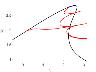
(a) $q=7,p=1$

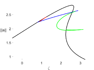
(b) $q=6,p=3$

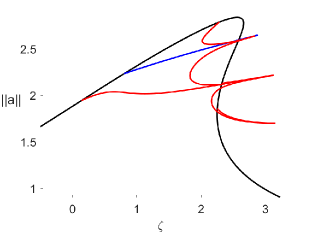
(c) $q=6,p=2$

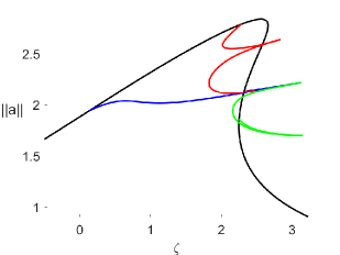
(d) $q=4,p=2$

Figure 4. $\mathcal{T}$ (black), primary branches (blue), secondary branches (green,red)

see Proposition 4.3 [21]. In particular, (A2) is satisfied. In a neighbourhood of these bifurcation points the associated Rabinowitz continua consist of $2\pi/k$-periodic solutions, and they are bounded and therefore return to $\mathcal{T}$ at some other bifurcation point. This analysis benefits from the fact that the sufficient conditions of the Crandall-Rabinowitz Theorem (A3),(A4),(A5) are satisfied in all bifurcation points for “generic” $d$ and $f$. This follows from the fact that the assumptions (S),(T) from Theorem 1.4 in [21] hold for most parameter values. The numerical investigations from Section 5.3 [21] suggest that the periodic pattern close to the bifurcation point may be lost along some of the bifurcating branches via secondary bifurcation. In the following we show how this phenomenon may be proved with the aid of Theorem 3. Our theoretical results are illustrated in Figure 4 using the Matlab software package pde2path.

Index computations

We apply Theorem 3 for the Banach spaces

(10) $$X=H^{1}_{per}\big{(}\frac{2\pi}{p};\mathbb{C}\big{)},\quad Y=H^{1}_{per}\big{(}\frac{2\pi}{q};\mathbb{C}\big{)}\qquad\text{where }p\text{ divides }q.$$

Since we will not encounter bifurcation from turning points of $\mathcal{T}$ later, we only consider $\xi=0$. For all bifurcation points $(\bar{a}(t_{k,i}),\bar{\zeta}(t_{k,i}))\in\mathcal{C}_{Y}\cap\mathcal{T}$ with $k\in q\mathbb{N}$ we will have to compute

(11) $$\delta^{*}_{X}(\bar{a}(t_{k,i}),\bar{\zeta}(t_{k,i});0)=\operatorname{sign}(\bar{\zeta}^{\prime}(t_{k,i}))\cdot(\iota_{X}(t_{k,i}+\varepsilon)-\iota_{X}(t_{j}-\varepsilon))\qquad(i=1,2),$$

see (4), where $\iota_{X}(t)$ is given by

$$\iota_{X}(t):=\operatorname{ind}_{X}(F(\cdot,\bar{\zeta}(t)),\bar{a}(t))=\operatorname{ind}_{X}(F_{a}(\bar{a}(t),\bar{\zeta}(t)),0).$$

Given the definition of the Leray-Schauder index and the fact that all eigenvalues are simple, the quantities $\iota_{X}(t_{k,i}+\varepsilon),\iota_{X}(t_{k,i}-\varepsilon)$ can be computed by counting the negative eigenvalues of the linearized operator $F_{a}(\bar{a}(t),\bar{\zeta}(t))[\cdot]:X\to X$. These eigenvalues can be computed with the aid of Proposition 4.3 [21]. In the notation from [21] one finds that $E$ is an eigenvalue of this operator in $X$ if and only if the determinant of one the matrices $dl^{2}\operatorname{Id}-N(a,\zeta)-E(dl^{2}+\operatorname{sign}(d))\operatorname{Id}$ for $l\in p\mathbb{N}$ vanishes. Plugging in the formula for $N(a,\zeta)$ from Proposition 4.2 [21] we get that the eigenvalues satisfy

(12) $$(\bar{\zeta}(t)+dl^{2}-E(dl^{2}+\operatorname{sign}(d)))^{2}-4|\bar{a}(t)|^{2}(\bar{\zeta}(t)+dl^{2}-E(dl^{2}+\operatorname{sign}(d)))+1+3|\bar{a}(t)|^{4}=0$$

for some $l\in p\mathbb{N}$ coming with $2\pi/l-$periodic eigenfunctions. So $\iota_{X}(t_{k,i}\pm\varepsilon)$ is the number of negative $E$ solving (12) for some $l\in p\mathbb{N}$, which can be computed rather easily using a computer. Notice that the eigenvalues change with $p$ and hence with the ambient space $X$.

Computing $\mathcal{C}_{Y}\cap\mathcal{T}$

Above we pointed out that all bifurcation points in $H^{1}_{per}([0,2\pi];\mathbb{C})$ are of the form $(\bar{a}(t_{k,1}),\bar{\zeta}(t_{k,1})),(\bar{a}(t_{k,2}),\bar{\zeta}(t_{k,2}))$ for $k=1,\ldots,k_{max}$ with $2\pi/k$-periodic eigenfunctions of the (simple) zero eigenvalue. Choosing $Y$ as in (10) we find that these points, being bifurcation points in $Y$, can belong to $\mathcal{C}_{Y}$ only if $k\in q\mathbb{N}$. So the choice $k_{max}/2<q\leq k_{max}$ ensures $k=q$. In particular, $\mathcal{C}_{Y}\cap\mathcal{T}\subset\{(\bar{a}(t_{q,1}),\bar{\zeta}(t_{q,1})),(\bar{a}(t_{q,2}),\bar{\zeta}(t_{q,2}))\}$. Moreover, $\mathcal{C}_{Y}$ is bounded by the a priori bounds from Theorem 1.1 and Theorem 1.2 in [21], so that the set $\mathcal{C}_{Y}\cap\mathcal{T}$ contains at least two elements by Rabinowitz’ bifurcation theorem, see (5) and the explanations thereafter. From these two facts we deduce

(13) $$\mathcal{C}_{Y}\cap\mathcal{T}=\{(\bar{a}(t_{q,1}),\bar{\zeta}(t_{q,1})),(\bar{a}(t_{q,2}),\bar{\zeta}(t_{q,2}))\}\qquad\text{provided }q\in\mathbb{N},\,k_{max}/2<q\leq k_{max}.$$

Summary

For generic $d\neq 0$ and $f\in\mathbb{R}$ we find $k_{max}\in\mathbb{N}_{0}$ such that the curve of constant solutions $\mathcal{T}$ given by (8) contains $2k_{max}$ bifurcation points in $H^{1}_{per}([0,2\pi];\mathbb{C})$ at $t=t_{k,1}$ or $t=t_{k,2}$ for $k=1,\ldots,k_{max}$. Choosing then $X,Y$ as in (10) with $k_{max}/2<q\leq k$ we get (13). The sufficient condition (6) for symmetry breaking secondary bifurcation can then be verified using (11) where the Leray-Schauder indices $\iota_{X}(t_{j}\pm\varepsilon)$ is $-1$ to the number of negative $E$ solving (12) for some $l\in p\mathbb{N}$.

Secondary bifurcations

For simplicity we now focus on a special case. We choose $f=1.6,d=0.1$ so that the interested reader may compare our results to those presented in Section 5.3 of the paper [21]. In this particular case the equation (9) has exactly 14 solutions, two for each $k\in\{1,\ldots,7\}$, i.e., $k_{max}=7$. The numerical values for these solutions $t_{k,1},t_{k,2}$ yielding the bifurcation points $(\bar{a}(t_{k,1}),\bar{\zeta}(t_{k,1})),(\bar{a}(t_{k,2}),\bar{\zeta}(t_{k,2}))$ in the ambient space $H^{1}_{per}([0,2\pi];\mathbb{C})$ are provided in Figure 3.

	$k=1$	$k=2$	$k=3$	$k=4$	$k=5$	$k=6$	$k=7$
$t_{k,1}$	$~{}0.10528$	$-0.18543$	$-0.52046$	$-0.72866$	$-0.77281$	$-0.6169$5	$-0.20600$
$t_{k,2}$	$~{}0.77130$	$~{}0.75556$	$~{}0.72127$	$~{}0.66089$	$~{}0.56321$	$~{}0.40312$	$~{}0.01535$
$\bar{\zeta}(t_{k,1})$	$~{}2.63750$	$~{}2.28327$	$~{}1.25702$	$~{}0.13682$	$-0.18666$	$~{}0.80166$	$~{}2.24085$
$\bar{\zeta}(t_{k,2})$	$~{}2.24888$	$~{}2.25196$	$~{}2.26952$	$~{}2.32248$	$~{}2.42954$	$~{}2.58449$	$~{}2.57475$
$\operatorname{Re}(\bar{a}(t_{k,1}))$	$~{}0.64816$	$~{}0.68661$	$~{}0.76763$	$~{}0.90117$	$~{}1.09247$	$~{}1.34000$	$~{}1.59962$
$\operatorname{Im}(\bar{a}(t_{k,1}))$	$-0.78546$	$-0.79192$	$-0.79934$	$-0.79358$	$-0.74462$	$-0.59026$	$-0.02455$
$\operatorname{Re}(\bar{a}(t_{k,2}))$	$~{}1.58226$	$~{}1.54499$	$~{}1.16659$	$~{}0.75049$	$~{}0.64442$	$~{}0.99099$	$~{}1.53210$
$\operatorname{Im}(\bar{a}(t_{k,2}))$	$-0.16752$	$~{}0.29154$	$~{}0.71106$	$~{}0.79847$	$~{}0.78473$	$~{}0.77687$	$~{}0.32253$

Figure 3. Bifurcation points on $\mathcal{T}$ for $f=1.6,d=0.1$

For notational convenience we write $z_{k,i}:=(\bar{a}(t_{k,i}),\bar{\zeta}(t_{k,i}))$ for the bifurcation points in $H^{1}_{per}([0,2\pi];\mathbb{C})$. Using (13) it is possible to check the symmetry breaking condition (6) with the aid of formula (11). Doing so for the spaces $X,Y$ from (10), Theorem 3 yields the following:

• $q=7,p=1$: Then $\delta_{X}^{*}(z_{7,1})+\delta_{X}^{*}(z_{7,2})=-4$, so the symmetry-breaking condition (6) from Theorem 3 is satisfied and secondary bifurcation from $(\mathcal{T},\mathcal{C}_{Y})$ occurs via period-septupling.

• $q=6,p=3$: Here we find $\delta_{X}^{*}(z_{6,1})+\delta_{X}^{*}(z_{6,2})=-4$, which implies secondary bifurcation by period-doubling from $2\pi/6-$periodic into $2\pi/3$-periodic solutions. Moreover, $\delta_{X}^{*}(z_{3,1})=\delta_{X}^{*}(z_{3,2})=2$ implies $\mathcal{C}_{X}\cap\mathcal{T}=\{z_{6,1},z_{6,2},z_{3,1},z_{3,2}\}$ because of Lemma 1 (ii). Item (3) even reveals that in a larger space, for instance in $H^{1}_{per}([0,2\pi];\mathbb{C})$, we will discover further secondary bifurcations.

• $q=6,p=2$: Then $\delta_{X}^{*}(z_{6,1})+\delta_{X}^{*}(z_{6,2})=4$, so secondary bifurcation via period-tripling occurs.

• $q=4,p=2$: From $\delta_{X}^{*}(z_{4,1})+\delta_{X}^{*}(z_{4,2})=-4$ we deduce secondary bifurcation via period-doubling.

In particular, we conclude: for $f=1.6,d=0.1$ and each pair $(q,p)\in\{(7,1),(6,3),(6,2),(4,2)\}$ there is a sequence of $2\pi/p$-symmetric but not $2\pi/q$-symmetric solutions of (7) converging to a nonconstant $2\pi/q$-symmetric solution.

5. Appendix A: Proof of Theorem 1

We finally provide the proof of Dancer’s and Rabinowitz’ results from Theorem 1 under the relaxed assumptions (A1),(A2). As in [10, 25] the main arguments rely on well-known properties of the Leray-Schauder degree. We refer to the survey article [23] and the books [1, 13] for more information about these topics. The following property will be especially important.

Lemma 2 (Generalized homotopy invariance).

Let $X$ be a real Banach space, $\Omega\subset X\times\mathbb{R}$ open and bounded and $F\in C(\overline{\Omega};X)$ a compact perturbation of the identity. If $F(x,t)\neq 0$ for all $x\in\partial\Omega_{t}$ with $t\in[0,1]$, then $t\mapsto d(F(\cdot,t),\Omega_{t},0)$ is constant on $[0,1]$.

For a proof of this well-known result we refer to Theorem 4.1 in [1]. We mention that $\Omega_{t}:=\{x\in X:(x,t)\in\Omega\}$, $t\in\mathbb{R}$, denote the slices of $\Omega$. Moreover, the projection of $\Omega$ onto the parameter space will be denoted by $\operatorname{pr}(\Omega):=\{t\in\mathbb{R}:\Omega_{t}\neq\emptyset\}$. Furthermore, we recall the following result, cf. Lemma 29.1 [13].

Lemma 3 (Whyburn).

Let $(M,d)$ be a compact metric space, $A\subset M$ a component and $B\subset M$ closed such that $A\cap B=\emptyset$. Then there exist compact $M_{A}\supset A,M_{B}\supset B$ such that $M=M_{A}\cup M_{B}$ and $M_{A}\cap M_{B}=\emptyset$.

Proof of Theorem 1:  We assume that $\mathcal{C}$ is bounded. Exploiting the discreteness of the set of bifurcation points $\Xi\subset\mathcal{T}$, see Proposition 1, we find that $\mathcal{C}\cap\mathcal{T}$ is finite and

(14) $$\overline{B_{\rho}(\mathcal{C})}\cap\Xi =\mathcal{C}\cap\mathcal{T}=\{(x_{ij},\lambda_{i}):i=0,\ldots,k,\,j=0,\ldots,m_{i}\}$$

where $\rho>0$ is sufficiently small, $k\in\mathbb{N}_{0}$,$m_{0},\ldots,m_{k}\in\mathbb{N}_{0}$ and the trivial solutions $(x_{ij},\lambda_{i})$ are all different from each other. Without loss of generality we may assume $\lambda_{0}<\lambda_{1}<\ldots<\lambda_{k}$. Here, $B_{\rho}(\mathcal{C}):=\{(x,\lambda)\in X\times\mathbb{R}:\operatorname{dist}((x,\lambda),\mathcal{C})<\rho\}$ denotes the open ball in $X\times\mathbb{R}$ around $\mathcal{C}$. Replacing $F,\mathcal{T}$ by $\tilde{F},\tilde{\mathcal{T}}$ given by

(15) $$\tilde{F}(x,\lambda):=F(x,\lambda+\langle\xi,x\rangle_{X^{\prime}}),\qquad\tilde{\mathcal{T}}:=\{(x,\lambda-\langle\xi,x\rangle_{X^{\prime}}):(x,\lambda)\in\mathcal{T}\}$$

we may without loss of generality assume that $\mathcal{C}\cap\mathcal{T}$ does not have turning points so that $\xi=0$ is transverse to $\mathcal{C}\cap\mathcal{T}$. So it remains to prove (5) in this special case. Due to the absence of turning points in $\mathcal{C}\cap\mathcal{T}$ we have (eventually after shrinking $\rho>0$)

$$(\mathcal{T}\cap\overline{B_{\rho}(\mathcal{C})}\setminus\mathcal{C})_{\lambda_{i}}=\emptyset\quad\text{ for }i=0,\ldots,k.$$

Since $\mathcal{S}\cap\overline{B_{\rho}(\mathcal{C})}$ is compact, we may invoke Whyburn’s Lemma to get $\mathcal{S}\cap\overline{B_{\rho}(\mathcal{C})}=K_{1}\cup K_{2}$ where $K_{1},K_{2}$ are disjoint compact sets such that $\mathcal{C}\subset K_{1}$ and $\mathcal{S}\cap\partial B_{\rho}(\mathcal{C})\subset K_{2}$. Then, for $0<\delta<\min\{\operatorname{dist}(K_{1},K_{2}),\operatorname{dist}(K_{1},\partial B_{\rho}(\mathcal{C}))\}$, the open set $\mathcal{O}:=B_{\delta}(K_{1})\subset B_{\rho}(\mathcal{C})$ is a bounded open neighbourhood of $\mathcal{C}$ satisfying

• $\partial\mathcal{O}\cap\mathcal{S}=\emptyset$ and $(\partial\mathcal{O}\cap\mathcal{T})_{\lambda_{i}}=\emptyset$ for $i=0,\ldots,k$,

• $\overline{\mathcal{O}}\cap\Xi=\mathcal{C}\cap\mathcal{T}$ is given by (14).

Next we define for $\lambda\in\mathbb{R}\setminus\{\lambda_{0},\ldots,\lambda_{k}\}$

$$\mu(\lambda) :=\lim_{r\to 0^{+}}d(F(\cdot,\lambda),B_{r}(\mathcal{T})_{\lambda},0),$$

$$\nu(\lambda) :=\lim_{r\to 0^{+}}d(F(\cdot,\lambda),(\mathcal{O}\setminus\overline{B_{r}(\mathcal{T})})_{\lambda},0).$$

Then $\mu(\lambda)$ is well-defined since $\mathcal{T}_{\lambda}$ does not contain a bifurcation point due to $\lambda\in\mathbb{R}\setminus\{\lambda_{0},\ldots,\lambda_{k}\}$ and (ii). Similarly, $\nu(\lambda)$ is well-defined in view of $\partial\mathcal{O}\cap\mathcal{S}=\emptyset$ by construction of $\mathcal{O}$. We now prove the following equalities for sufficiently small $\varepsilon>0$:

• $\mu(\lambda_{i}-\varepsilon)+\nu(\lambda_{i}-\varepsilon)=\mu(\lambda_{i}+\varepsilon)+\nu(\lambda_{i}+\varepsilon)$ for $i=0,\ldots,k$,

• $\nu(\lambda_{i}+\varepsilon)=\nu(\lambda_{i+1}-\varepsilon)$ for $i=0,\ldots,k-1$,

• $\nu(\lambda_{0}-\varepsilon)=0$ and $\nu(\lambda_{k}+\varepsilon)=0$.

Choose $\varepsilon>0$ such that $B_{r}(\mathcal{T})_{\lambda}\subset\mathcal{O}_{\lambda}$ for $|\lambda-\lambda_{i}|\leq\varepsilon$. Then, by (i), $\partial O_{\lambda}$ does not contain any zeros of $F(\cdot,\lambda)$ whenever $|\lambda-\lambda_{i}|\leq\varepsilon$. Hence, the additivity and the homotopy invariance of the degree yield

$$\mu(\lambda_{i}-\varepsilon)+\nu(\lambda_{i}-\varepsilon) =d(F(\cdot,\lambda_{i}-\varepsilon),\mathcal{O}_{\lambda_{i}-\varepsilon},0)$$

$$=d(F(\cdot,\lambda_{i}+\varepsilon),\mathcal{O}_{\lambda_{i}+\varepsilon},0)$$

$$=\mu(\lambda_{i}+\varepsilon)+\nu(\lambda_{i}+\varepsilon).$$

This proves (a). By property (ii) there is a sufficiently small $r>0$ such that solutions $(x,\lambda)\in\mathcal{O}$ with $\lambda_{i}+\varepsilon\leq\lambda\leq\lambda_{i+1}-\varepsilon$ for $i=0,\ldots,k-1$ satisfy $(x,\lambda)\notin\overline{B_{r}(\mathcal{T})}$ and $(x,\lambda)\notin\partial O\setminus B_{r}(\mathcal{T})$ follows from property (i). So, Lemma 2 implies for $i=0,\ldots,k-1$

$$\nu(\lambda_{i}+\varepsilon) =d(F(\cdot,\lambda_{i}+\varepsilon),(\mathcal{O}\setminus\overline{B_{r}(\mathcal{T})})_{\lambda_{i}+\varepsilon},0)$$

$$=d(F(\cdot,\lambda_{i+1}-\varepsilon),(\mathcal{O}\setminus\overline{B_{r}(\mathcal{T})})_{\lambda_{i+1}-\varepsilon},0)$$

$$=\nu(\lambda_{i+1}-\varepsilon)$$

so that (b) is proved, too. Claim (c) follows again from Lemma 2 and the fact that $\mathcal{O}$ is bounded. Indeed, for all $r>0$ we have

(16) $$d(F(\cdot,\lambda),(\mathcal{O}\setminus\overline{B_{r}(\mathcal{T})})_{\lambda},0)=d(F(\cdot,\lambda),\emptyset,0)=0\quad\;\text{if }\lambda\leq\lambda_{*}:=\inf\operatorname{pr}(\mathcal{O}).$$

As above, by (i) and (ii) we may choose $r>0$ such that all solutions $(x,\lambda)\in\overline{\mathcal{O}}$ with $\lambda_{*}\leq\lambda\leq\lambda_{0}-\varepsilon$ satisfy $(x,\lambda)\notin\overline{B_{r}(\mathcal{T})}$ as well as $(x,\lambda)\notin\partial O\setminus B_{r}(\mathcal{T})$. Hence, we get from (16)

$$\nu(\lambda_{0}-\varepsilon)=d(F(\cdot,\lambda_{0}-\varepsilon),(\mathcal{O}\setminus\overline{B_{r}(\mathcal{T})})_{\lambda_{0}-\varepsilon},0)=d(F(\cdot,\lambda_{*}),(\mathcal{O}\setminus\overline{B_{r}(\mathcal{T})})_{\lambda_{*}},0)=0.$$

The analogous reasoning gives $\nu(\lambda_{k}+\varepsilon)=0$.

From (a),(b),(c) we deduce

$$\sum_{i=0}^{k}\big{(}\mu(\lambda_{i}+\varepsilon)-\mu(\lambda_{i}-\varepsilon)\big{)} =-\sum_{i=0}^{k}\big{(}\nu(\lambda_{i}+\varepsilon)-\nu(\lambda_{i}-\varepsilon)\big{)}$$

$$=\nu(\lambda_{k}-\varepsilon)-\sum_{i=0}^{k-1}\big{(}\nu(\lambda_{i}+\varepsilon)-\nu(\lambda_{i}-\varepsilon)\big{)}$$

$$=\nu(\lambda_{k}-\varepsilon)-\sum_{i=0}^{k-1}\big{(}\nu(\lambda_{i+1}-\varepsilon)-\nu(\lambda_{i}-\varepsilon)\big{)}$$

$$=\nu(\lambda_{k}-\varepsilon)-\nu(\lambda_{k}-\varepsilon)+\nu(\lambda_{0}-\varepsilon)$$

$$=0$$

so that it remains to rewrite this identity in the form (5). To this end we use that for $|\lambda-\lambda_{i}|\leq\varepsilon$ sufficiently small the slices $(\mathcal{O}\cap\mathcal{T})_{\lambda}$ consist of precisely $m_{i}+1$ distinct points that converge to the points $x_{ij},j=0,\ldots,m_{i}$ as $\lambda\to\lambda_{i}$. Notice that at this point we use that none of these points is a turning point of $\mathcal{T}$. Invoking the Leray-Schauder index formula (see for instance Theorem 8.10 in [13] or Lemma 3.19 in [1]) we arrive for $\varepsilon>0$ sufficiently small at

$$\mu(\lambda_{i}+\varepsilon)-\mu(\lambda_{i}-\varepsilon) =\sum_{(x,\lambda_{i}+\varepsilon)\in\mathcal{O}\cap\mathcal{T}}\operatorname{ind}(F(\cdot,\lambda_{i}+\varepsilon),x)-\sum_{(x,\lambda_{i}-\varepsilon)\in\mathcal{O}\cap\mathcal{T}}\operatorname{ind}(F(\cdot,\lambda_{i}-\varepsilon),x)$$

$$=\sum_{(x,\lambda_{i}+\varepsilon)\in\mathcal{O}\cap\mathcal{T}}\operatorname{ind}(F_{x}(x,\lambda_{i}+\varepsilon),0)-\sum_{(x,\lambda_{i}-\varepsilon)\in\mathcal{O}\cap\mathcal{T}}\operatorname{ind}(F_{x}(x,\lambda_{i}-\varepsilon),0)$$

$$=\sum_{j=0}^{m_{i}}\delta^{*}(x_{ij},\lambda_{i};0).$$

These identities finally imply

$$0=\sum_{i=0}^{k}\big{(}\mu(\lambda_{i}+\varepsilon)-\mu(\lambda_{i}-\varepsilon)\big{)}=\sum_{i=0}^{k}\sum_{j=0}^{m_{i}}\delta^{*}(x_{ij},\lambda_{i};0)=\sum_{(x,\lambda)\in\mathcal{C}\cap\mathcal{T}}\delta^{*}(x,\lambda;0).$$

$\Box$

6. Appendix B: On assumption (A2)

In this Section we motivate the assumption of locally uniform differentiability of $F$ along the trivial solution $\mathcal{T}$ in the context of Proposition 1. We provide an example for a not locally uniformly differentiable function $F:X\times\mathbb{R}\to X$ with $F(0,\lambda)=0$ for all $\lambda\in\mathbb{R}$ such that the set of bifurcation points is not discrete even though the set of degenerate solutions on $\mathcal{T}$ is. In particular, this shows that Proposition 1 cannot hold without this assumption.

The starting point for the construction of a counterexample is a differentiable function $f:\mathbb{R}\times\mathbb{R}\to\mathbb{R}$ with $f|_{\mathcal{T}}=0$ such that $f$ is not locally uniformly differentiable along $\mathcal{T}$, but $\lambda\mapsto f^{\prime}(0,\lambda)$ is continuous. We define $M:=\max_{z\in\mathbb{R}}\sin^{2}(z)/z>0$ and its unique maximizer $z^{*}\approx 1.165561$. Then the following function has the above-mentioned properties:

$$f(x,\lambda):=x-M^{-1}\sin^{2}(x\lambda^{-3})\lambda^{3}\quad\text{for }x\in\mathbb{R},\lambda\neq 0,\qquad f(x,0):=x\quad\text{for }x\in\mathbb{R}$$

Moreover, we have $f_{x}(0,\lambda)=1$ for all $\lambda\in\mathbb{R}$ and $(0,0)$ is a bifurcation point because of $f(x_{\lambda},\lambda)=0$ for all $\lambda\in\mathbb{R}$ where $x_{\lambda}:=z^{*}\lambda^{3}$. Notice that there are no other nontrivial solutions. We conclude:

$$(0,0)\text{ is a bifurcation point for }f(x,\lambda)=0\text{ with }f_{x}(0,0)\neq 0.$$

In other words $(0,0)$ is a nondegenerate bifurcation point for this equation in the sense we defined at the beginning of Section 2. We stress that this is possible due to the fact that $f$ is not locally uniformly differentiable along $\mathcal{T}$ and in particular not continuously differentiable in a neighbourhood of $\mathcal{T}$. In fact, one has $x_{\lambda}\to 0$ as $\lambda\to 0$ and

$$\frac{f(x_{\lambda},\lambda)-f(0,\lambda)-f_{x}(0,\lambda)x_{\lambda}}{x_{\lambda}}=\frac{\sin^{2}(x_{\lambda}\lambda^{-3})}{Mx_{\lambda}\lambda^{-3}}=\frac{\sin^{2}(z^{*})}{Mz^{*}}=1\not\to 0\quad\text{as }\lambda\to 0.$$

In the next Lemma, this function is used for the construction of a counterexample.

Lemma 4.

There is a differentiable function $F:\mathbb{R}\times\mathbb{R}\to\mathbb{R}$ satisfying $F(0,\lambda)=0$ for all $\lambda\in\mathbb{R}$ and such that the following holds for $\lambda_{0}\in\mathbb{R}$:

• The map $\lambda\mapsto F^{\prime}(0,\lambda)$ is continuous on $\mathbb{R}$,

• $F_{x}(0,\lambda_{0})=0$ and $F_{x}(0,\lambda)(\lambda-\lambda_{0})>0$ for all $\lambda\neq\lambda_{0}$,

• there is a sequence of bifurcation points $(0,\lambda_{n})$ for $F(x,\lambda)=0$ s.t. $\lambda_{n}\to\lambda_{0}$ as $n\to\infty$.

Proof.

W.l.o.g. we may assume $\lambda_{0}=0$. Let $f$ be defined as above, let $\chi\in C_{0}^{\infty}(\mathbb{R})$ be a smooth cut-off function such that $\chi(z)=1$ for $|z|\leq\frac{1}{2}$, $0<\chi(z)<1$ for $|z|<1$ and $\chi(z)=0$ for $|z|\geq 1$ and define

$$F(x,\lambda) :=\lambda\Big{(}\sum_{k\in\mathbb{Z}}\chi(a2^{k}(\lambda-2^{-k}))f(x,\lambda-2^{-k})+\sum_{k\in\mathbb{Z}}\chi(a2^{k}(\lambda+2^{-k}))f(x,\lambda+2^{-k})\Big{)}$$

where $a\in(2,3)$. Our aim is to verify the above-mentioned properties for $\lambda_{n}:=2^{-n}$. First let us mention that the $k$-th summand in the first series may not be zero only if $\lambda\in(\frac{a-1}{a}2^{-k},\frac{a+1}{a}2^{-k})$. So, for all $\lambda>0$ we can find a small open neighbourhood of $\lambda$ and $k_{\lambda}\in\mathbb{Z}$ such that the second sum is zero and the $k$-th summand in the first series vanishes on this neighbourhood whenever $k\notin\{k_{\lambda},k_{\lambda}+1\}$. Here, $a>1$ is used. The analogous reasoning applies to $\lambda<0$. So the well-definedness and differentiability of $F$ at points $(0,\lambda)$ with $\lambda\neq 0$ follows from the corresponding statements about $f$. Moreover, we have $F(0,\lambda)=0$ for all $\lambda\in\mathbb{R}$. Let us prove the claims (i)–(iii).

Proof of (i): For $\lambda\neq 0$ we have $F_{\lambda}(0,\lambda)=0$ and

(17) $$F_{x}(0,\lambda)=\lambda\Big{(}\sum_{k\in\mathbb{Z}}\chi(a2^{k}(\lambda-2^{-k}))+\sum_{k\in\mathbb{Z}}\chi(a2^{k}(\lambda+2^{-k}))\Big{)}.$$

So (i) is proved once we show that $F^{\prime}(0,0)$ exists with $F_{x}(0,0)=F_{\lambda}(0,0)=0$. Indeed, we have for $x,\lambda\to 0$

$$|F(x,\lambda)| \leq|\lambda|\sum_{k\in\mathbb{Z}}\big{(}|\chi(a2^{k}(\lambda-2^{-k}))||f(x,\lambda-2^{-k})|+|\chi(a2^{k}(\lambda+2^{-k}))||f(x,\lambda+2^{-k})|\big{)}$$

$$\leq 2|\lambda||x|\sum_{k\in\mathbb{Z}}\big{(}|\chi(a2^{k}(\lambda-2^{-k}))|+|\chi(a2^{k}(\lambda+2^{-k}))|\big{)}$$

$$\leq 4|\lambda||x|\;=\;o(|x|+|\lambda|).$$

Here we used that $\chi(a2^{k}(\lambda\pm 2^{-k}))$ is non-zero for at most two indices $k$.

Proof of (ii): For any given $\lambda>0$ we can choose $k\in\mathbb{Z}$ such that $\lambda\in(\frac{a-1}{a}2^{-k},\frac{a+1}{a}2^{-k})$. This is due to $a<3$. So $\chi(a2^{k}(\lambda-2^{-k}))>0$ and thus $F_{x}(0,\lambda)\lambda>0$ in view of  (17). The analogous reasoning applies to $\lambda<0$, which implies (ii).

Proof of (iii): We show that bifurcation occurs at $\lambda_{n}=2^{-n}$. Indeed, for $0<|\lambda|\leq\min\{\frac{a-1}{2a},\frac{a-2}{a}\}2^{-n}$, which is possible due to $a>2$, we have

$$a2^{k}|(2^{-n}+\lambda)-2^{-k}| =a|2^{k-n}(1-2^{n}\lambda)-1|\geq a\Big{(}2\cdot\big{(}1-\frac{a-1}{2a}\big{)}-1\Big{)}=1 \text{if }k>n,$$

$$a2^{k}|(2^{-n}+\lambda)-2^{-k}| \geq a\big{(}1-2^{k}(|\lambda|+2^{-n})\big{)}\geq a\Big{(}1-2^{k}\cdot\frac{2a-2}{a}2^{-n}\Big{)}\geq a\big{(}1-\frac{a-1}{a}\big{)}=1 \text{if }k<n.$$

The same inequalities hold for $a2^{k}|(2^{-n}+\lambda)+2^{-k}|$ and all $k\in\mathbb{Z}$. So we get

$$F(x_{\lambda},2^{-n}+\lambda) =(2^{-n}+\lambda)\Big{[}\sum_{k\in\mathbb{Z}}\underbrace{\chi(a2^{k}(2^{-n}+2^{-k}+\lambda))}_{=0}f(x_{\lambda},2^{-n}+2^{-k}+\lambda)$$

$$\qquad\quad\quad+\sum_{k\in\mathbb{Z},k\neq n}\underbrace{\chi(a2^{k}(2^{-n}-2^{-k}+\lambda))}_{=0}f(x_{\lambda},2^{-n}-2^{-k}+\lambda)$$

$$\qquad\quad\quad+\chi(a2^{n}\lambda)\underbrace{f(x_{\lambda},\lambda)}_{=0}\Big{]}$$

$$=0.$$

Hence, $(0,\lambda_{n})$ is a bifurcation point, which is all we had to show. $\Box$

References

- [1] A. Ambrosetti and A. Malchiodi. Nonlinear analysis and semilinear elliptic problems, volume 104 of Cambridge Studies in Advanced Mathematics. Cambridge University Press, Cambridge, 2007.
- [2] T. Bartsch, E. N. Dancer, and Z.-Q. Wang. A Liouville theorem, a-priori bounds, and bifurcating branches of positive solutions for a nonlinear elliptic system. Calc. Var. Partial Differential Equations, 37(3-4):345–361, 2010.
- [3] T. Bartsch, R. Tian, and Z.-Q. Wang. Bifurcations for a coupled Schrödinger system with multiple components. Z. Angew. Math. Phys., 66(5):2109–2123, 2015.
- [4] L. Bauer, H. B. Keller, and E. L. Reiss. Multiple eigenvalues lead to secondary bifurcation. SIAM Rev., 17:101–122, 1975.
- [5] R. Böhme. Die Lösung der Verzweigungsgleichungen für nichtlineare Eigenwertprobleme. Math. Z., 127:105–126, 1972.
- [6] J. Bracho, M. Clapp, and W. Marzantowicz. Symmetry breaking solutions of nonlinear elliptic systems. Topol. Methods Nonlinear Anal., 26(1):189–201, 2005.
- [7] G. Cerami. Symmetry breaking for a class of semilinear elliptic problems. Nonlinear Anal., 10(1):1–14, 1986.
- [8] C. V. Coffman. A nonlinear boundary value problem with many positive solutions. J. Differential Equations, 54(3):429–437, 1984.
- [9] M. G. Crandall and P. H. Rabinowitz. Bifurcation from simple eigenvalues. J. Functional Analysis, 8:321–340, 1971.
- [10] E. N. Dancer. On the structure of solutions of non-linear eigenvalue problems. Indiana Univ. Math. J., 23:1069–1076, 1973/74.
- [11] E. N. Dancer. Breaking of symmetries for forced equations. Math. Ann., 262(4):473–486, 1983.
- [12] E. N. Dancer. Global breaking of symmetry of positive solutions on two-dimensional annuli. Differential Integral Equations, 5(4):903–913, 1992.
- [13] K. Deimling. Nonlinear functional analysis. Springer-Verlag, Berlin, 1985.
- [14] B. Gidas, W. M. Ni, and L. Nirenberg. Symmetry and related properties via the maximum principle. Comm. Math. Phys., 68(3):209–243, 1979.
- [15] H. Kielhöfer. Bifurcation theory, volume 156 of Applied Mathematical Sciences. Springer, New York, second edition, 2012. An introduction with applications to partial differential equations.
- [16] M. A. Krasnosel’skii. Topological methods in the theory of nonlinear integral equations. The Macmillan Co., New York, 1964.
- [17] K. Kuto, T. Mori, T. Tsujikawa, and S. Yotsutani. Secondary bifurcation for a nonlocal Allen-Cahn equation. J. Differential Equations, 263(5):2687–2714, 2017.
- [18] S.-S. Lin. On non-radially symmetric bifurcation in the annulus. J. Differential Equations, 80(2):251–279, 1989.
- [19] L. A. Lugiato and R. Lefever. Spatial dissipative structures in passive optical systems. Phys. Rev. Lett., 58:2209–2211, 1987.
- [20] R. Mandel. Grundzustände, Verzweigungen und singuläre Lösungen nichtlinearer Schrödingersysteme. PhD thesis, Karlsruhe Institute of Technology (KIT), 2013.
- [21] R. Mandel and W. Reichel. A priori bounds and global bifurcation results for frequency combs modeled by the Lugiato-Lefever equation. SIAM J. Appl. Math., 77(1):315–345, 2017.
- [22] A. Marino. La biforcazione nel caso variazionale. Confer. Sem. Mat. Univ. Bari, (132):14, 1973.
- [23] J. Mawhin. Leray-Schauder degree: a half century of extensions and applications. Topol. Methods Nonlinear Anal., 14(2):195–228, 1999.
- [24] Y. Miyamoto. Non-existence of a secondary bifurcation point for a semilinear elliptic problem in the presence of symmetry. J. Math. Anal. Appl., 357(1):89–97, 2009.
- [25] P. H. Rabinowitz. Some global results for nonlinear eigenvalue problems. J. Functional Analysis, 7:487–513, 1971.
- [26] J. Smoller and A. G. Wasserman. Bifurcation and symmetry-breaking. Invent. Math., 100(1):63–95, 1990.
- [27] P. N. Srikanth. Symmetry breaking for a class of semilinear elliptic problems. Ann. Inst. H. Poincaré Anal. Non Linéaire, 7(2):107–112, 1990.