Sub-voxel perfusion modeling in terms of coupled 3$d$-1$d$ problem

Abstract

We study perfusion by a multiscale model coupling diffusion in the tissue and diffusion along the one-dimensional segments representing the vasculature. We propose a block-diagonal preconditioner for the model equations and demonstrate its robustness by numerical experiments. We compare our model to a macroscale model by [P. Tofts, Modelling in DCE MRI, 2012].

1 Introduction

The micro-circulation is altered in diseases such as cancer and Alzheimer’s disease, as demonstrated with modern perfusion MRI. In cancer, the so-called enhanced permeability and retention (EPR) effect describes the fact that the smaller vessels in a tumor are leaky, highly permeable vessels that enable the tumor cells to grow quicker than normal cells.

In Alzheimer’s disease (AD), the opposite is alleged to happen. According to [8], hypoperfusion is a precursor to AD, and the cause of the pathological cell-level changes occuring in AD. This could also explain why various kinds of heart disease are risk factors for AD, as changes in the blood pressure would affect the perfusion of the brain.

The vasculature (e.g. idealized as a system of pipes) and the surrounding tissue are clearly three-dimensional. However, the fact that in many applications the radii of the vessels are negligible compared to their lengths, permits reducing their governing equations to models prescribed on (one dimensional) curves where the physical radius $R$ enters as a parameter. In this paper, we consider a coupled 3$d$-1$d$ system

$$\frac{\partial u}{\partial t} =D_{\Omega}\Delta_{\Omega}u+\delta_{\Gamma}\beta\lambda \quad\text{ in }\Omega,$$

$$\frac{\partial\hat{u}}{\partial t} =D_{\Gamma}\Delta_{\Gamma}\hat{u}-\beta\lambda \quad\text{ in }\Gamma,$$ (1)

$$\lambda =\beta(\Pi_{R}u-\hat{u}) \text{ in }\Gamma.$$

Here, $\delta_{\Gamma}$ is the Dirac measure on $\Gamma$; $u$, $\hat{u}$ are the concentrations in the tissue domain $\Omega$ and the one-dimensional vasculature representation $\Gamma$; and $D_{\Omega}$, $D_{\Gamma}$ are conductivities on the respective domains. The last equation is then a generalized Starling’s law; relating $\hat{u}$ and the value $\Pi_{R}u$ of $u$ averaged over the idealized cylindrical vessel surface centered around $\Gamma$. The equation thus represents a coupling between the domains.

Variants of the system (1) have been used to study coupling between tissue and vasculature flow in numerous applications. In [7], a steady state limit of the system is used to numerically investigate oxygen supply of the skeletal muscles. Finite differences were used for the discretization. Using the method of Green’s functions, [17], [18] and [3] studied oxygen transport in the brain and tumors. Transport of oxygen inside the brain was also investigated by [12] using the finite volume method (FVM) and [6] using the finite element method (FEM) for the 3$d$ diffusion problem and FVM elsewhere. In these studies the 1$d$ problem was transient. More recently, coupled models discretized entirely by FEM were applied to study cancer therapies, see e.g. [15] and references therein. The mathematical foundations of these works are rooted in the seminal contributions of [5], [4] where well-posedness of the following problem is analyzed

$$-\Delta_{\Omega}u+(\hat{u}-\Pi_{R}u)\delta_{\Gamma}=f\delta_{\Gamma} \quad\text{ in }\Omega$$ (2)

$$-\Delta_{\Gamma}\hat{u}-(\hat{u}-\Pi_{R}u)=g \quad\text{ in }\Gamma.$$

The presence of the measure term in (2) requires the use of non-standard spaces in the analysis. In [5], the variational formulation of the problem is proven to be well-posed using weighted Sobolev spaces. In particular, the solution $u$ is sought in $H^{1}_{\alpha}(\Omega)$, $\alpha>0$ while the test functions $v$ for the first equation in (2) are taken from $H^{1}_{-\alpha}(\Omega)$. With this choice, the right-hand side $\langle f\delta_{\Gamma},v\rangle$ as well as the trace operator $v\mapsto v|_{\Gamma}$ are well defined, while the reduced regularity of $u$ is sufficient to for the average $\Pi_{R}u$ to make sense. As shown in [4], use of FEM for the formulation in weighted spaces yields optimal rates if the computational mesh is gradually refined towards $\Gamma$ (graded meshes).

Another approach to the analysis of (2) has recently been suggested in the numerical study [2]. Building on the analysis of [9] for the elliptic problem with a 0 dimensional Dirac right-hand side, the wellposedness of the problem was shown with trial spaces $W^{1,p}(\Omega)$, $p=3-\tfrac{d}{2}$ and test spaces $W^{1,q}(\Omega)$, $p^{-1}+q^{-1}=1$, and quasi-optimal error estimates for FEM shown in the norms which excluded a fixed neighborhood of $\Gamma$ of radius $R$.

In studying AD or EPR, the physical parameters may vary across several orders of magnitude while small or large time steps can be desirable depending on the time scales of interest. The solution algorithm for the employed model equations is thus required to be robust with respect to these parameters as well independent of the discretization. For (the transient version of) (2) the construction of such algorithms is complicated by the non-standard spaces on the domain $\Omega$.

A potential remedy for the problem can be introduction of a Lagrange multiplier which enforces the coupling between the domains with the goal of confining the non-standard spaces to the smaller domain $\Gamma$. This idea has been used by [11] to analyze robust preconditioners for 2$d$-1$d$ coupled problems based on operators in fractional Sobolev spaces, in particular, $(-\Delta_{\Gamma})^{\scalebox{0.5}{$-\tfrac{1}{2}$}}$, while numerical experiments reported in [10] suggest that for suitable exponents $(-\Delta_{\Gamma})^{s}$ defines a preconditioner for the Schur complement of a 3$d$-1$d$ coupled system with a trace constraint. We note that in both cases off-the-shelf methods were used as preconditioners for the operators on $\Omega$.

The system (1) includes an additional variable $\lambda$ for the coupling constraint, cf. (2). We therefore aim to apply the techiques of [10], [11] to construct a mesh-independent preconditioner for the problem, while the ideas of operator preconditioning [14] are used to ensure robustness with respect to the physical parameters and the time-stepping.

The rest of the paper is organized as follows. Section 2 identifies the structure of the preconditioner. In §3 we discuss discretization of the proposed operator and report numerical experiments which demonstrate the robust properties. In §4 the system (1) is used to model tissue perfusion using a realistic geometry of the rat cortex. Conclusions are finally summarized in §5.

2 Preconditioner for the coupled problem

In the following we let $\Omega$ be a bounded domain in $\mathbb{R}^{d}$, $d=2$ or 3 and $\Gamma$ be a subdomain of $\Omega$ of dimension 1. By $L_{2}(D)$ we denote the space of square-integrable functions over $D$ and $H^{1}(D)$ is the space of functions with first order derivatives in $L^{2}(D)$.

Discretizing (1) in time by backward-Euler discretization the problem to be solved at each temporal level is of the form

$$\mathcal{A}u=f$$

with

$$\mathcal{A}=\left[\begin{array}[]{ccc}I-kD_{\Omega}\Delta_{\Omega}&0&k\beta\Pi_{R}^{*}\\ 0&I-kD_{\Gamma}\Delta_{\Gamma}&k\beta I\\ k\beta\Pi_{R}&k\beta I&-k.\end{array}\right]$$ (3)

and $k$ being the time step size. Note that in order to obtain a symmetric problem the operator $\mathcal{A}$ uses the adjoint $\Pi_{R}^{*}$ of the averaging operator $\Pi_{R}$ instead of the trace, cf. (1). The choice results in modeling error of order $\mathcal{O}(R)$.

To motivate the structure of the preconditioner let us consider a $3\times 3$ matrix

$$A=\left[\begin{array}[]{ccc}1+\alpha_{1}&0&\beta_{1}\\ 0&1+\alpha_{2}&\beta_{2}\\ \beta_{1}&\beta_{2}&-\gamma\end{array}\right]$$

where $\alpha_{1}$, $\alpha_{2}$, $\beta_{1}$, $\beta_{2}$, and $\gamma$ are assumed to be positive. It can then be shown that with

$$B=\left[\begin{array}[]{ccc}(1+\alpha_{1})^{-1}&0&0\\ 0&(1+\alpha_{2})^{-1}&0\\ 0&0&(\gamma+\beta_{1}^{2}+\beta_{2}^{2})^{-1}+(\gamma+\beta_{1}^{2}/\alpha_{1}+\beta_{2}^{2}/\alpha_{2})^{-1}\end{array}\right]$$

the condition number of $BA$ is bounded independent of the parameters. With this in mind we propose that $\mathcal{A}$ can be preconditioned by a block-diagonal operator

$$\mathcal{B}=\left[\begin{array}[]{ccc}(I-kD_{\Omega}\Delta_{\Omega})^{-1}&0&0\\ 0&(I-kD_{\Gamma}\Delta_{\Gamma})^{-1}&0\\ 0&0&S\end{array}\right],$$ (4)

where

$$S=S^{-1}_{1}+S_{2}^{-1}$$ (5)

and

$$S_{1} =\gamma I+(k\beta)^{2}\Pi_{R}\Pi_{R}^{*}+(k\beta)^{2}I,$$ (6)

$$S_{2} =\gamma I+(k\beta)^{2}\Pi_{R}(-kD_{\Omega}\Delta_{\Omega})^{-1}\Pi_{R}^{*}+(k\beta)^{2}(-kD_{\Gamma}\Delta_{\Gamma})^{-1}.$$

The operator $\mathcal{B}$ could be rigorously derived within operator preconditioning [14] as a Riesz map preconditioner for $\mathcal{A}$ viewed as an isomorphism from $V(\Omega)\times\hat{V}(\Gamma)\times Q(\Gamma)$ to its dual space. In [11] the framework was applied to a system of two elliptic problems coupled by a 2$d$-1$d$ constraint. For (1) extension of the analysis to parabolic problems would be required. In [13] robust preconditioners for time-dependent Stokes problem were analyzed as operators between sums of (parameter) weighted Sobolev spaces. Similarly, the structure of (5) suggests that $Q=Q_{1}+Q_{2}$ with $Q_{1}$, $Q_{2}$ being suitable interpolation spaces. However, here we shall not justify $Q_{1}$ and $Q_{2}$ (and the preconditioner $\mathcal{B}$) theoretically. Instead, $Q_{1}$, $Q_{2}$ are characterized and robustness of $\mathcal{B}$ is demonstrated by numerical experiments.

3 Discrete preconditioner

Considering $\eqref{kam_eq:opB}$, both $(I-kD_{\Omega}\Delta_{\Omega})^{-1}$ and $(I-kD_{\Gamma}\Delta_{\Gamma})^{-1}$ can be realized with off-the-shelf multilevel algorithms and the crucial question is thus how to construct $S$ efficiently. Note that assembling $S_{1}$ and in particular $S_{2}$ might be too costly or even prohibitive, cf. $(-\Delta_{\Omega})^{-1}$ in $S_{2}$. However, following (6) the preconditioner can be realized if operators spectrally equivalent to $\Pi_{R}(-\Delta_{\Omega})^{-1}\Pi_{R}^{*}$ and $\Pi_{R}\Pi_{R}^{*}$ are known and if the inverse (action) of the resulting approximations to $S_{1}$ and $S_{2}$ is inexpensive to compute.

3.1 Auxiliary operators

If $\Omega\subset\mathbb{R}^{2}$ and $\Pi_{R}$ is understood as the trace operator, the mapping properties of trace as a bounded surjective operator $H^{1}(\Omega)\rightarrow H^{\scalebox{0.5}{$\tfrac{1}{2}$}}(\Gamma)$ can be used to show that $\Pi_{R}(-\Delta_{\Omega})^{-1}\Pi_{R}^{*}$ is spectrally equivalent with $(-\Delta_{\Gamma})^{\scalebox{0.5}{$-\tfrac{1}{2}$}}$. At the same time $\Pi_{R}\Pi_{R}^{*}=\Pi_{R}(-\Delta)^{0}_{\Omega}\Pi_{R}^{*}$ requires characterizing the space of traces of functions in $L^{2}{(\Omega)}$. We shall demonstrate by a numerical experiment that a spectrally equivalent operator is here provided by an operator $h^{-1}I_{h}$.

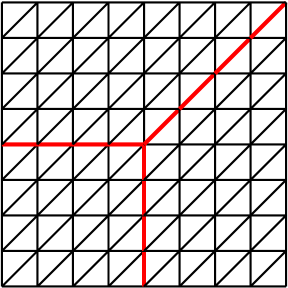
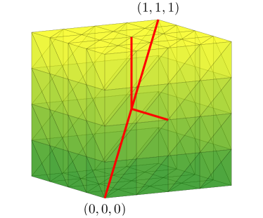
Figure 1: Geometries used in preconditioning numerical experiments. The domain is $\Omega=\left[0,1\right]^{d}$ while in order to prevent symmetries $\Gamma$ (pictured in red) always features a branching point. Triangulation of $\Gamma$ is made up of edges of the cells that triangulate $\Omega$.

Let $\Omega_{h},\Gamma_{h}$ be triangulations of $\Omega$ and $\Gamma$ such that $\Gamma_{h}$ consists of a subset of edges of the elements $\Omega_{h}$, cf. Figure 1. Further let $V_{h},Q_{h}$ be finite element spaces of continuous linear Lagrange elements on $\Omega_{h}$ and $\Gamma_{h}$ respectively. Finally we consider the eigenvalue problem: Find $\lambda\in\mathbb{R}$, $u\in V_{h}$, $p\in Q_{h}$ such that

$$\int_{\Omega}uv+\int_{\Gamma}p\Pi_{R}v =\lambda\int_{\Omega}uv \quad\forall v\in V_{h},$$ (7)

$$\int_{\Gamma}q\Pi_{R}u =\lambda\int_{\Gamma}h^{-1}pq \quad\forall q\in Q_{h}.$$

Table 1 shows the spectral condition number $\kappa=\max{\lvert\lambda\rvert}/\min{\lvert{\lambda}\rvert}$ of the linear systems (7). For all the considered resolutions $h$ the value of $\kappa$ is bounded.

As the mapping properties of $\Pi_{R}\Pi_{R}^{*}$ and $\Pi_{R}(-\Delta_{\Omega})^{-1}\Pi_{R}^{*}$ in case $\Omega\subset\mathbb{R}^{3}$ are not trivially obtained from the continuous analysis, we again resort to finding the suitable approximations by numerical experiments. Similar to the two dimensional case, the first operator with $\Pi_{R}$ having the constant radius $R=0.02$ is found to be spectrally equivalent with $h^{-1}I_{h}$. Following [10], an approximation to $\Pi_{R}(-\Delta_{\Omega})^{-1}\Pi_{R}^{*}$ is searched for as a suitable power $s<0$ of $(-\Delta_{\Gamma}+I_{\Gamma})$. More precisely, we look for the exponent yielding the most $h$-stable condition number of the eigenvalue problem: Find $\lambda\in\mathbb{R}$, $u\in V_{h}$, $p\in Q_{h}$ such that

$$\int_{\Omega}\nabla u\cdot\nabla v+\int_{\Gamma}p\Pi_{R}v =\lambda\int_{\Omega}\nabla u\nabla v+uv \quad\forall v\in V_{h},$$ (8)

$$\int_{\Gamma}q\Pi_{R}u =\lambda\int_{\Gamma}p(-\Delta_{\Gamma}+I_{\Gamma})^{s}q \quad\forall q\in Q_{h}.$$

In (8) the powers are computed using the spectral decomposition of the operator $-\Delta_{\Gamma}+I_{\Gamma}$.

We shall not present here the results for the entire optimization problem and only report on the optimum which is found to be $s=-0.55$. For this value Table 1 shows the history of the condition numbers of system (8) using again $R=0.02$. There is a slight growth by a constant increment on the finer meshes, however, the final condition number is comparable with that obtained on the coarsest mesh. We note that we have not investigated the behaviour of the exponent on different curves or with variable radius. This subject is left for future works.

	$\Omega\subset\mathbb{R}^{2}$						$\Omega\subset\mathbb{R}^{3}$
	$1/h$						$1/h$
	32	64	128	256	512	1024	4	8	16	32	64	128
eq. (7)	4.36	4.33	4.35	4.36	4.36	4.35	4.26	5.22	5.58	4.44	4.85	4.85
eq. (8)	8.80	8.84	8.84	8.86	8.88	8.87	11.04	8.25	7.44	9.02	10.30	11.25

Table 1: Spectral condition numbers of the eigenvalue problems related to approximations of $\Pi_{R}\Pi_{R}^{*}$(eq (7)) and $\Pi_{R}(-\Delta_{\Omega})\Pi_{R}^{*}$(eq (8)). In the two-dimensional case (8) uses $s=-\tfrac{1}{2}$ in agreement with the mapping properties of the continuous trace operator. Results for $s=-0.55$ are reported in the three dimensional case. On the finest triangulation $\dim V_{h}\sim 10^{6}$ and $\dim Q_{h}\sim 10^{3}$ when $d=2$ and $\dim Q_{h}\sim 10^{2}$ for $d=3$.

3.2 Discrete preconditioner for the coupled problem

Applying the proposed preconditioner (4) of the coupled 3$d$-1$d$ problem (3) requires evaluating the inverse of operators $S_{1}$ and $S_{2}$ in (6). The former is readily computed since, due to the suggested equivalence of $\Pi_{R}\Pi_{R}^{*}$ and $h^{-1}I_{h}$, the matrix representation of $S_{1}$ is essentialy a rescaled mass matrix. For $S_{2}$ we show that if $(-\Delta_{\Gamma}+I_{\Gamma})^{s}$ is computed from the spectral decomposition then the inverse $S^{-1}_{2}$ can be computed in a closed form.

Let $A$, $M$ be the $n\times n$ matrix representations of Galerkin approximations of $-\Delta_{\Gamma}+I_{\Gamma}$ and $I$ in the space $Q_{h}\subset H^{1}(\Gamma)$. Following [11] the matrix representation of $(-\Delta_{\Gamma}+I_{\Gamma})_{h}^{s}$ is $H_{s}=MU\Lambda^{s}(MU)^{\prime}$ where the matrices $U$, $\Lambda$ solve the generalized eigenvalue problem $AU=MU\Lambda$ such that $U^{\prime}MU=I$. Using $H_{s}$ it is easily established that the matrix representation of $S_{2}$ is

$$\gamma H_{0}+(k\beta)^{2}(kD_{\Omega})^{-1}H_{-\frac{1}{2}}+(k\beta)^{2}(kD_{\Gamma})^{-1}H_{-1}.$$

As $H^{-1}_{s}=U\Lambda^{-s}U^{\prime}$ the inverse of the $S_{2}$ matrix is given by

$$U\left(\gamma\Lambda^{0}+(k\beta)^{2}(kD_{\Omega})^{-1}\Lambda^{-\frac{1}{2}}+(k\beta)^{2}(kD_{\Gamma})^{-1}\Lambda^{-1}\right)^{-1}U^{\prime}.$$ (9)

Using the spectral decomposition, the cost of setting up the preconditioner $S$ is determined by the cost of solving the generalized eigenvalue problem for $U$ and $\Lambda$. This practically limits the construction to systems where $\dim Q_{h}\sim 10^{3}$. However, for the problems considered further, this limitation does not present an issue. In particular, the preconditioner can be setup on the discretization of vasculature of the cortex tissue used in §4 which contains approximately twenty thousand vertices.

With a discrete approximation of $S$ we can finally address the question of $\mathcal{B}$ being a robust preconditioner for (3). Motivated by (1) we do not vary all the paramaters, and instead, set $\gamma=1$ in $\mathcal{A}$. Morever, the conductivity on $\Omega$ is taken as unity and only variable $D_{\Gamma}>1$ is considered mimicking the expected faster propagation along the one-dimensional domain. Finally, the time step $k$ and the coupling constant $\beta$ shall take values between $10^{-4}$ and $10^{-8}$.

For a fixed choice of parameters $D_{\Gamma}$, $\beta$, $k$, the preconditioned problem $\mathcal{B}\mathcal{A}x=\mathcal{B}f$ is considered on geometries from Figure 1 and discretized with continuous linear Lagrange elements. The resulting linear system is then solved with the MinRes method where the iterations are stopped once the preconditioned residual norm is less than $10^{-10}$ in magnitude.

The observed iteration counts are reported in Table 2. For both 2$d$-1$d$ and 3$d$-1$d$ coupled problems the iterations can be seen to be bounded in the discretization parameter. Moreover the preconditioner performs almost uniformly in the considered ranges of $D_{\Gamma}$ and $\beta$ while there is a clear boundedness in $k$ as well. We note that these conclusions are not significantly altered if the ranges for $k$ and $\beta$ are extended to 1.

$D_{\Gamma}$	$\beta$	$k$	2$d$-1$d$						3$d$-1$d$
			$1/h$						$1/h$
			32	64	128	256	512	1024	4	8	16	32	64	128
$10^{0}$	$10^{-8}$	$10^{-8}$	11	10	10	8	7	7	8	13	12	11	11	10
		$10^{-6}$	15	13	12	10	8	8	10	14	16	16	15	13
		$10^{-4}$	16	11	12	13	13	14	12	16	18	16	13	14
	$10^{-6}$	$10^{-8}$	11	10	10	8	7	7	8	13	12	11	11	10
		$10^{-6}$	15	13	12	10	8	8	10	14	16	16	15	13
		$10^{-4}$	15	11	12	13	13	14	12	16	18	16	13	14
	$10^{-4}$	$10^{-8}$	11	10	10	8	7	7	8	13	12	11	11	10
		$10^{-6}$	15	13	12	10	8	8	10	14	16	16	15	13
		$10^{-4}$	16	11	12	13	13	14	12	16	18	16	13	14
$10^{2}$	$10^{-8}$	$10^{-8}$	11	10	10	9	7	7	8	13	12	11	11	10
		$10^{-6}$	15	13	12	10	8	8	10	14	16	16	15	13
		$10^{-4}$	15	11	12	13	13	13	11	16	18	13	13	14
	$10^{-6}$	$10^{-8}$	11	10	10	9	7	7	8	13	12	11	11	10
		$10^{-6}$	15	13	12	10	8	8	10	14	16	16	15	13
		$10^{-4}$	15	11	12	13	13	13	11	16	18	13	13	14
	$10^{-4}$	$10^{-8}$	11	10	10	9	7	7	8	13	12	11	11	10
		$10^{-6}$	15	13	12	10	8	8	10	14	16	16	15	13
		$10^{-4}$	15	11	12	13	13	13	12	16	18	13	13	14
$10^{4}$	$10^{-8}$	$10^{-8}$	11	10	10	8	7	7	8	13	12	11	11	10
		$10^{-6}$	15	13	12	10	8	8	10	14	16	16	15	13
		$10^{-4}$	15	11	12	13	12	10	11	16	18	13	13	14
	$10^{-6}$	$10^{-8}$	11	10	10	8	7	7	8	13	12	11	11	10
		$10^{-6}$	15	13	12	10	8	8	10	14	16	16	15	13
		$10^{-4}$	15	11	12	13	12	10	11	16	18	13	13	14
	$10^{-4}$	$10^{-8}$	11	10	10	8	7	7	8	13	12	11	11	10
		$10^{-6}$	15	13	12	10	8	8	10	14	16	16	15	13
		$10^{-4}$	15	11	12	13	12	10	11	16	18	13	13	14
$10^{6}$	$10^{-8}$	$10^{-8}$	11	10	10	8	7	7	8	13	12	11	11	10
		$10^{-6}$	15	13	12	10	8	8	10	14	16	16	15	13
		$10^{-4}$	14	10	10	9	8	5	11	15	18	13	11	11
	$10^{-6}$	$10^{-8}$	11	10	10	8	7	7	8	12	12	11	11	10
		$10^{-6}$	15	13	12	10	8	8	10	14	16	16	15	13
		$10^{-4}$	14	10	10	9	8	5	11	15	18	13	10	11
	$10^{-4}$	$10^{-8}$	11	10	10	8	7	7	8	12	12	11	11	10
		$10^{-6}$	15	13	12	10	8	8	10	14	16	16	15	13
		$10^{-4}$	14	10	10	9	8	5	11	16	18	13	10	11

Table 2: Number of iterations of MinRes method on (3) using (4) as preconditioner with $S$ approximated using (9). (Left) 2$d$-1$d$ coupled problem and (right) 3$d$-1$d$ coupled problem from Figure 1 are considered.

Having demonstrated the numerical stability of our model, we next test it on the same problem as [19], namely a bloodborne tracer perfusing and later being cleared from tissue. While [19] considers this problem on a macroscopic scale, we model it on the micro-scale, where individual blood vessels can be resolved as part of our 1$d$ domain.

4 Perfusion experiment

In [16], a $0.7\text{mm}\times 0.7\text{mm}\times 0.7\text{mm}$ piece of mouse brain microvasculature was imaged using two-photon microscopy. To obtain a realistic geometry for our model, we used this data to generate a 3$d$ mesh of the extravascular space in which vessel segments corresponded to 1$d$ mesh edges. The radius of the blood vessels is used as the radius $R$ in the definition of the averaging operator $\Pi_{R}$, and ranged between $1$ and $15$ micron.

To model a small region of tissue being perfused by a bloodborne tracer, we use initial conditions of $u,\hat{u}=0$, and a boundary condition of $\hat{u}=1\>\frac{\text{mol}}{\text{L}}$ on the part of the boundary corresponding to inlet vessels. To model clearance, the inlet boundary condition was swapped from $\hat{u}=1$ to $\hat{u}=0$ after a third of the simulation time had passed.

As parameters, we use $D_{\Gamma}=6.926\times 10^{7}\>\mu\text{m}^{2}/\text{s}$, $D_{\Omega}=1.87\times 10^{2}\>\mu\text{m}^{2}/\text{s}$ and $\beta=50\>\mu\text{m}/\text{s}$. We used $k=1\text{s}$ after verifying that reducing it did not significantly affect our results. In this experiment, it was unneccessary to use the preconditioner described in §3 since the problem size was small enough to allow for use of a direct solver.

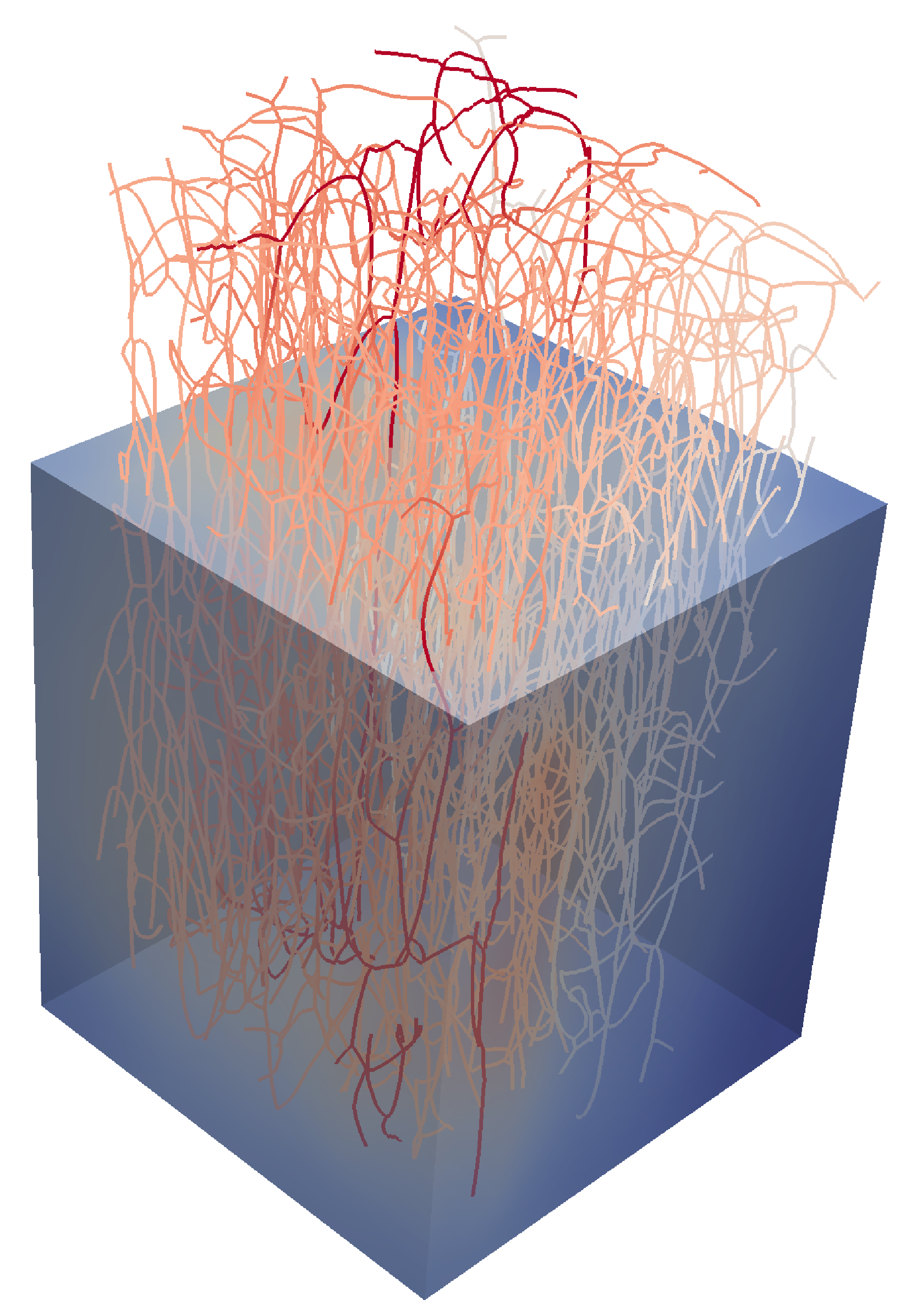
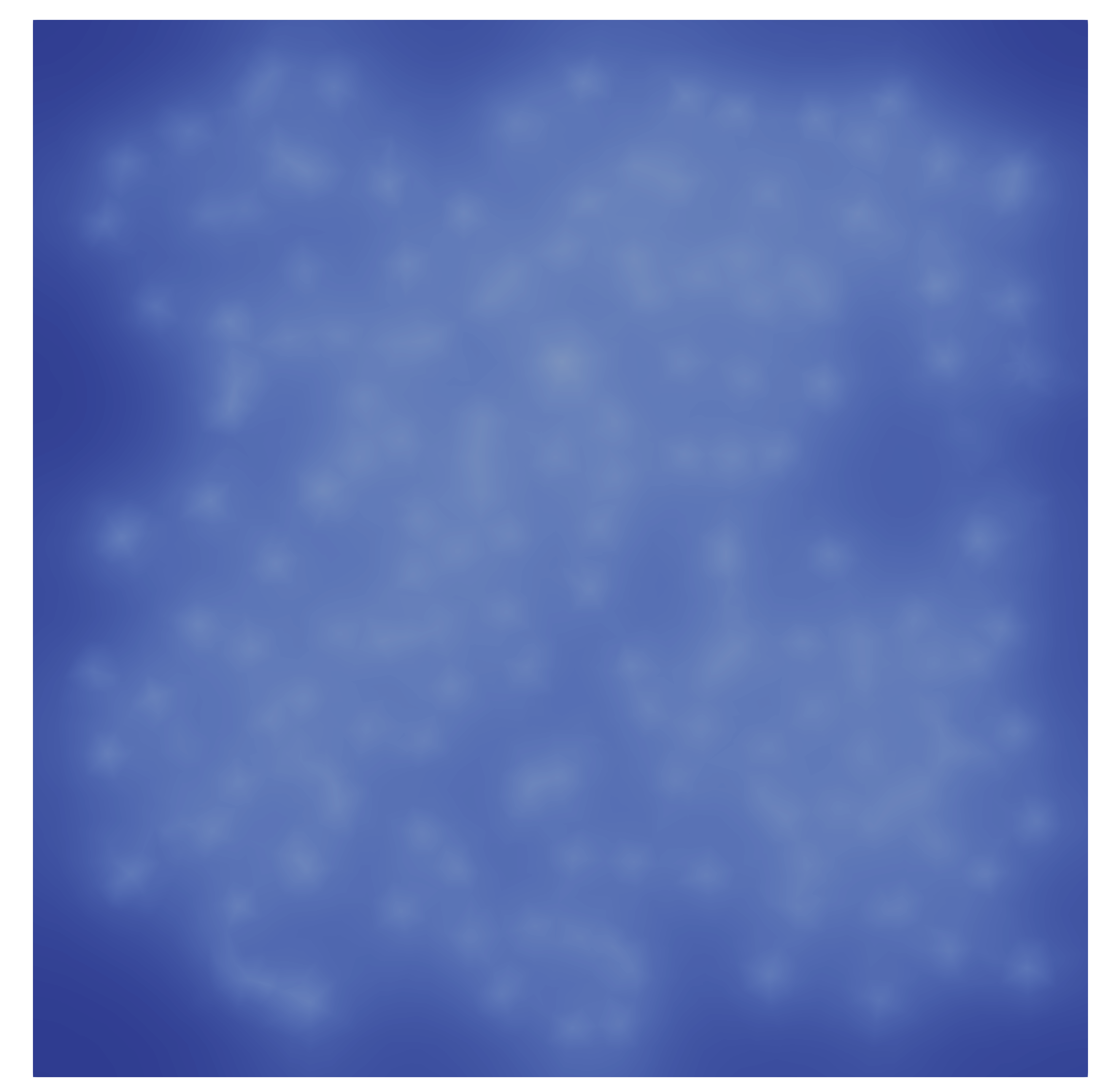
Figure 2: Example results shown on a (left) clip of the 3$d$ domain and (right) on a slice. Notice the ’halos’ of increased concentration immediately around the vessels.

Tofts [19] assumes a relation

$$\frac{\partial C_{t}}{\partial t}=\frac{K_{\text{trans}}}{\nu}(C_{v}-C_{t})$$ (10)

between the pixel tissue concentration $C_{t}$ and the pixel vessel concentration $C_{v}$ for some constant $K_{\text{trans}}$. Here, $\nu$ is the vascular volume fraction, which in our geometry is about $0.76\%$. Our geometry is of a size comparable to a single pixel in [19], so $C_{t}$ and $C_{v}$ correspond to the normalized averages

$$C_{t}=\frac{\int_{\Omega}u}{\int_{\Omega}1}\quad\mbox{and}\quad C_{v}=\frac{\int_{\Gamma}\pi R^{2}\hat{u}}{\int_{\Gamma}\pi R^{2}}.$$

We computed $K_{\text{trans}}$ by solving for $u,\hat{u}$ using our model, and then computing $C_{t},C_{v}$ as given above, and defining $K_{\text{trans}}$ such that equation (10) holds at each time point. This makes $K_{\text{trans}}$ a function of time, with units $\text{seconds}^{-1}$.

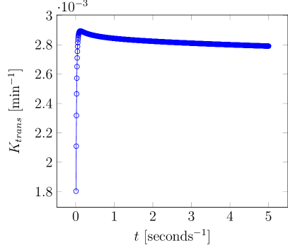
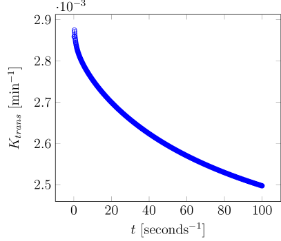
Figure 3: Behavior of $K_{\text{trans}}$ on short and long time scales.

4.1 Discussion of perfusion experiment

Our value for $K_{\text{trans}}$ is not entirely constant. There is a small variation in time, as perfusion seems to be somewhat faster when the extravascular space is completely empty of the tracer. As it starts getting saturated, perfusion slows down somewhat. This translates into $K_{\text{trans}}$ decreasing by about $20\%$ over a period of about 5 minutes, from 0.0028 $\text{min}^{-1}$ to 0.0023 $\text{min}^{-1}$.

In [20], $K_{\text{trans}}$ was estimated in healthy and cancerous human brain tissue from MRI scans. In healthy tissue, they estimate $K_{\text{trans}}$ to be between 0.003 $\text{min}^{-1}$ and 0.005 $\text{min}^{-1}$, that is, slightly higher than our results. There are several possible explanations for this difference. One might be that in our model, vascular transport is modeled as exceptionally fast diffusion for convenience, whereas in reality it occurs by convection. However, in both cases 1$d$ transport is very fast compared to the 3$d$ transport and the 1$d$-3$d$ exchange. Further, $K_{\text{trans}}$ is defined in terms of the 1$d$-3$d$ exchange alone, so non-extreme variations in the 1$d$ transport seem unlikely to be relevant.

Another possibility might be that the data of [20] are taken from human brain tissue, while our vasculature is taken from a mouse brain tissue, likely from a different region of the brain. A third reason might be our diffusion constants not exactly matching the tracer used by [20].

In further work, it would be interesting to incorporate convective transport into the model and see if better agreement with the experimental data is observed. A suitable starting point here is [1], who derive a convection-diffusion type system (equations (3a), (3b)) by assuming that the blood flow $\hat{q}$ in a segment is laminar and follows Poiseuille’s law

$$\hat{q}=R^{4}C\nabla{\hat{p}}.$$

4.2 Parameter sensitivity analysis

We carried out a rudimentary parameter sensitivity analysis by varying the three parameters $D_{\Gamma},D_{\Omega},\beta$ by a factor 10 and seeing how that affected the tissue concentration $C_{t}$. Specifically, we started from a baseline of
$D_{\Gamma}=6.926\cdot 10^{8}\>\frac{\mu m^{2}}{s},D_{\Omega}=1.87\cdot 10^{2}\>\frac{\mu m^{2}}{s},\beta=5\cdot 10^{1}\>\text{s}^{\scalebox{0.5}{$-\tfrac{1}{2}$}}$, and for each parameter, increased or decreased it by a factor 10.

The results are shown in Figure 4. They indicate that $C_{t}$ depends more strongly on $\beta$ and $D_{\Gamma}$ than on $D_{\Omega}$ for the set of parameters considered here.

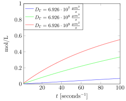
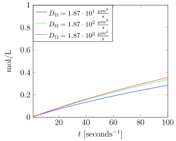
Figure 4: Plots of variation in $C_{t}$ when different parameters are varied.

5 Conclusions

A coupled 3$d$-1$d$ system with an additional unknown enforcing the coupling between the domains was used as a model of tissue perfusion. For the system we proposed a robust preconditioner and demonstrated its properties through numerical experiments. Further, we have shown that the model can be applied to a physiological problem with reasonable results.

References

- [1] L. Cattaneo and P. Zunino, A computational model of drug delivery through microcirculation to compare different tumor treatments, International journal for numerical methods in biomedical engineering 30:11 (2014), 1347–1371.
- [2] , Numerical investigation of convergence rates for the FEM approximation of 3D-1D coupled problems, Numerical Mathematics and Advanced Applications-ENUMATH 2013, Springer, 2015, pp. 727–734.
- [3] S. J. Chapman, R. J. Shipley, and R. Jawad, Multiscale modeling of fluid transport in tumors, Bulletin of Mathematical Biology 70:8 (2008), 2334.
- [4] C. D’Angelo, Finite element approximation of elliptic problems with Dirac measure terms in weighted spaces: applications to one-and three-dimensional coupled problems, SIAM Journal on Numerical Analysis 50:1 (2012), 194–215.
- [5] C. D’Angelo and A. Quarteroni, On the coupling of 1D and 3D diffusion-reaction equations: application to tissue perfusion problems, Mathematical Models and Methods in Applied Sciences 18:08 (2008), 1481–1504.
- [6] Q. Fang, S. Sakadžić, L. Ruvinskaya, A. Devor, A. M. Dale, and D. A. Boas, Oxygen advection and diffusion in a three dimensional vascular anatomical network, Optics express 16:22 (2008), 17530.
- [7] D. Goldman and A. S. Popel, A computational study of the effect of capillary network anastomoses and tortuosity on oxygen transport, Journal of Theoretical Biology 206:2 (2000), 181–194.
- [8] C. Jack, Cerebrovascular and cardiovascular pathology in Alzheimer’s disease, International Review of Neurobiology 84 (2009), 35–48.
- [9] T. Koppl and B. Wohlmuth, Optimal a priori error estimates for an elliptic problem with Dirac right-hand side, SIAM Journal on Numerical Analysis 52:4 (2014), 1753–1769.
- [10] M. Kuchta, K.-A. Mardal, and M. Mortensen, On preconditioning saddle point systems with trace constraints coupling 3D and 1D domains–applications to matching and nonmatching FEM discretizations, arXiv preprint arXiv:1612.03574 (2016).
- [11] M. Kuchta, M. Nordaas, J. C. Verschaeve, M. Mortensen, and K.-A. Mardal, Preconditioners for saddle point systems with trace constraints coupling 2D and 1D domains, SIAM Journal on Scientific Computing 38:6 (2016), B962–B987.
- [12] A. Linninger, I. Gould, T. Marinnan, C.-Y. Hsu, M. Chojecki, and A. Alaraj, Cerebral microcirculation and oxygen tension in the human secondary cortex, Annals of biomedical engineering 41:11 (2013), 2264–2284.
- [13] K.-A. Mardal and R. Winther, Uniform preconditioners for the time dependent Stokes problem, Numerische Mathematik 98:2 (2004), 305–327.
- [14] , Preconditioning discretizations of systems of partial differential equations, Numerical Linear Algebra with Applications 18:1 (2011), 1–40.
- [15] M. Nabil, P. Decuzzi, and P. Zunino, Modelling mass and heat transfer in nano-based cancer hyperthermia, Royal Society open science 2:10 (2015), 150447.
- [16] S. Sakadžić, E. T. Mandeville, L. Gagnon, J. J. Musacchia, M. A. Yaseen, M. A. Yucel, J. Lefebvre, F. Lesage, A. M. Dale, K. Eikermann-Haerter, et al., Large arteriolar component of oxygen delivery implies a safe margin of oxygen supply to cerebral tissue, Nature communications 5 (2014), 5734.
- [17] T. W. Secomb, R. Hsu, E. Y. Park, and M. W. Dewhirst, Green’s function methods for analysis of oxygen delivery to tissue by microvascular networks, Annals of biomedical engineering 32:11 (2004), 1519–1529.
- [18] T. Secomb, R. Hsu, N. Beamer, and B. Coull, Theoretical simulation of oxygen transport to brain by networks of microvessels: effects of oxygen supply and demand on tissue hypoxia, Microcirculation 7:4 (2000), 237–247.
- [19] P. S. Tofts, T1-weighted DCE imaging concepts: modelling, acquisition and analysis, Signal 500:450 (2010), 400.
- [20] N. Zhang, L. Zhang, B. Qiu, L. Meng, X. Wang, and B. L. Hou, Correlation of volume transfer coefficient with histopathologic grades of gliomas, Journal of Magnetic Resonance Imaging 36:2 (2012), 355–363.