M101: Spectral observations of H ii regions and their physical properties

Abstract

By using the Hectospec 6.5 m Multiple Mirror Telescope (MMT) and the 2.16 m telescope of National Astronomical Observatories, Chinese Academy of Sciences (NAOC), we obtained 188 high signal-to-noise ratio (S/N) spectra of H ii regions in the nearby galaxy M101, which are the largest spectroscopic sample of H ii regions for this galaxy so far. These spectra cover a wide range of regions on M101, which enables us to analyze two dimensional distributions of its physical properties. The physical parameters are derived from emission lines or stellar continuum, including stellar population age, electron temperature, oxygen abundance and etc. The oxygen abundances are derived using two empirical methods based on O3N2 and R₂₃ indicators, as well as the direct $T_{e}$ method when $\hbox{[O\,{\sc iii}]}\lambda 4363$ is available. By applying the harmonic decomposition analysis to the velocity field, we obtained line-of-sight rotation velocity of 71 $\rm{km~{}s}^{-1}$ and a position angle of 36 degree. The stellar age profile shows an old stellar population in galaxy center and a relative young stellar population in outer regions, suggesting an old bulge and a young disk. Oxygen abundance profile exhibits a clear break at $\sim$18 kpc, with a gradient of $-$0.0364 dex kpc^-1 in the inner region and $-$0.00686 dex kpc^-1 in the outer region. Our results agree with the “inside-out” disk growth scenario of M101.

1 Introduction

H ii regions are the sites of strong star formation in galaxies, which make H ii regions perfect probes of star formation processes, evolution of massive stars and the surrounding interstellar medium. Plenty of information can be obtained by analyzing the emission lines and underlying stellar continuum of their spectra. The gas-phase metallicity, defined as the number ratio of oxygen to hydrogen atom, is one of the key properties in galaxy formation and evolution. The oxygen is synthesized in high-mass stars (>8$M_{\sun}$) and then released to the inter-stellar medium through stellar winds or supernova explosion. The spatial distributions of the oxygen abundance in galaxies are affected by a variety of processes, such as enriched outflows (Tremonti et al., 2004), accretion (Dalcanton et al., 2004), and mergers (Kewley et al., 2006; Rupke et al., 2010; Kewley et al., 2010; Rich et al., 2012; Torrey et al., 2012; Sánchez et al., 2014). Thus studying the metallicity and its relation with other properties would provide clues on the galaxy formation and evolution.

Researches on the metallicity of H ii regions are booming in the last two decades. Zaritsky et al. (1994) and van Zee et al. (1998) found that H ii regions have an average metallicity gradient of $-$0.05 dex kpc^-1, i.e. the inner regions of galaxies are more metal-rich than the outskirts. The negative gradients are found to be universal, as reviewed by many following researches (Bresolin, 2007; Scarano & Lépine, 2013; Li et al., 2013; Sánchez et al., 2014; Ho et al., 2015; Sánchez et al., 2016b), suggesting inner-to-out transportation of metals. Observations also show breaks in the oxygen abundance gradients in a number of galaxies (Zaritsky, 1992; Roy & Walsh, 1997). Pilyugin (2003) claimed that such breaks are due to the systematic error involving the excitation parameter, while others attribute it to the barrier effect of corotation, which isolates the inner and outer regions of the disk one from the other due to opposite directions of gas flow (Lépine et al., 2011; Scarano & Lépine, 2013). More recently, several studies focusing on gas content have found that the metallicity gradients flatten to a constant value beyond the isophotal radii R₂₅ or 2R_e (Rosales-Ortega et al., 2011; Marino et al., 2012; Sánchez et al., 2012, 2014; López-Sánchez et al., 2015; Sánchez et al., 2016b), and several scenarios are proposed to explain the nature of this flattening, such as the bar induced radial gas flows (Cavichia et al., 2014), minor mergers and perturbations from satellite galaxies (Bird et al., 2012; López-Sánchez et al., 2015), the varying star formation efficiency over a large galacentric distances (Bresolin et al., 2012; Esteban et al., 2013), and the balance between outflows and inflows with the intergalactic medium (Oppenheimer & Davé, 2008; Oppenheimer et al., 2010; Davé et al., 2011, 2012).

Recently, the Integral Field Unit (IFU) spectrograph is becoming a most important and powerful tool for spatial-resolved spectroscopic observations, which has greatly increased the progress of the two-dimensional research on galaxies. Many surveys using IFU technology are carried out, such as SAURON (Bacon et al., 2001), PINGS (Rosales-Ortega et al., 2010), CALIFA (Sánchez et al., 2012) and MaNGA (Bundy et al., 2015) survey. According to their different observational strategies, MaNGA is mapping a large number of galaxies with limited spatial resolution (1-3 kpc) and field of view ($\sim$70 acrsec), while PIGNS provides a better spatial resolution and larger field of view but with limited number of galaxies, and CALIFA is a compromise between the two. Sánchez et al. (2014) found a common metallicity gradient of $-$0.10$\pm$0.09 dex R${}_{e}^{-1}$ for 193 CALIFA galaxies, and the metallicity gradients do not exhibit the dependence on other properties of galaxies, such as morphology, mass, and the presence or absence of bars (Sánchez et al., 2016b). By studying 49 local field star-forming galaxies, Ho et al. (2015) proposed a local benchmark of metallicity gradients of $-$0.39$\pm$0.18 dex R${}_{25}^{-1}$. More recently, Belfiore et al. (2017) analyzed 550 nearby galaxies from MaNGA survey and confirm that metallicity gradient is flat for low mass galaxies ($\hbox{$M_{*}$}<10^{9.0}\hbox{$M_{\sun}$}$), steepens for more massive galaxies until $\hbox{$M_{*}$}\sim 10^{10.5}\hbox{$M_{\sun}$}$ and flattens lightly again for even more massive galaxies. These researches provided strong constraints on galactic chemical composition of nearby galaxies (Chiappini et al., 2001; Fu et al., 2009; Ho et al., 2015; Sánchez et al., 2016b; Belfiore et al., 2017).

Kong et al. (2014) proposed the “Spectroscopic Observations of the H ii Regions In Nearby Galaxies (H2ING)” Project, which performs spectroscopic observations on H ii regions in 20 nearby large galaxies since 2008. As the third paper of this project, we report the spectroscopic observation of H ii regions in nearby galaxy M101, with the MMT 6.5 m telescope (Fabricant et al., 2005) and the NAOC 2.16 m telescope (Fan et al., 2016). M101 (also known as NGC 5457, $\alpha=14^{h}03^{m}12^{s}.5$, $\delta=+54^{\circ}20^{\prime}56^{\prime\prime}$) is a large face-on Scd galaxy containing plenty of H ii regions (Hodge et al., 1990; Kennicutt et al., 2003; Gordon et al., 2008; Bresolin, 2007; Croxall et al., 2016). It has a distance of about 7.4 Mpc and an apparent scale of about 36 pc arcsec^-1, which enables us to observe its H ii regions to a scale of a few hundred pc with our $1.5^{\prime\prime}$ fiber and $2.5^{\prime\prime}$ slit observations. A major-axis position angle of $39^{\circ}$ and an inclination angle of $18^{\circ}$ (Bosma et al., 1981) allow us to perform detailed studies of its stellar populations and ionized nebulae. Observations of the M101 H ii regions have been carried out since 1970s (Searle, 1971; Smith, 1975; McCall et al., 1985; Kennicutt & Garnett, 1996; Bresolin, 2007). Recently, Li et al. (2013) presented a catalog containing 79 H ii regions from their observations and several previous works since 1996. Croxall et al. (2016) have enlarged the sample of H ii regions by using the Large Binocular Telescope (LBT), and obtained 109 spectra of H ii regions in M101. In this paper, we have obtained 188 H ii region with high S/N from our observations, which is the largest spectroscopic sample of H ii regions for M101.

With the spectra of numerous H ii regions, we have derived the physical properties of H ii regions, and presented a detailed study of the spatial distribution of these properties. This paper is structured as follows. In Section 2, we describe the observation, data reduction and emission line measurements. In Section 3, we present the measurements and analysis of physical properties of the H ii region sample. Metallicities are derived with three methods and the gradient is also calculated and discussed. We summarize our results in Section 4.

2 Data

2.1 Observations

The H ii region candidates are selected from the continuum-subtracted H$\alpha$ image (Hoopes et al., 2001). Candidates are primarily selected with preference for large regions, using SExtractor (Bertin & Arnouts, 1996) with irregular area filter with at least 25-pixel (1 pixel $=2.028^{\prime\prime}$). The foreground stars are excluded from the H ii catalog by matching with the 2MASS all-sky Point Source Catalog (PSC; Cutri et al., 2003). Then candidates are observed with the Hectospec multi-fiber positioner and spectrograph on the 6.5 m MMT telescope and the NAOC 2.16 m telescope.

The usable field of the MMT 6.5 m telescope is 1° in diameter, and the instrument deployed three hundred $1.5^{\prime\prime}$-diameter fibers on the field, corresponding to $\sim$ 54 pc at the distance of M101. We used Hectospecs 270 gpm grating that provided a dispersion of 1.2 Å pixel^-1 and a resolution of $\sim$ 5 Å. The spectral wavelength coverage is from 3650 to 9200 Å. The Hectospec fiber assignment software xfitfibs allows the user to assign rankings to targets. If we ignored the spatial positions of our targets, fiber collisions would prevent many objects in the center portion of the center of M101 from being observed. We therefore assigned priority to H ii regions based on their H$\alpha$ fluxes. We observed two fields at the night on 2012 February 10 with 3600 s exposure times and one field on 2013 March 15 with 5400 s exposure times. Weather conditions are clear on both nights, and seeings are about $1.2^{\prime\prime}$, $0.8^{\prime\prime}$ and $0.6^{\prime\prime}$ for each field, respectively.

The NAOC 2.16 m telescope worked with an OMR (Optomechanics Research Inc.) spectrograph providing a dispersion of 4.8 Å pixel ^-1 and a resolution of 10 Å. The observed spectra cover the wavelength range of 3500 to 8100 Å. Slits of $2.5^{\prime\prime}$ are placed manually to cover as many candidates as possible and to avoid those observed by MMT. Observations are carried out over 9 nights between 2012 and 2014 with 20 slits, and exposure times varied between 3600 s and 5400 s depending on weather conditions. Typical seeing is $\sim 2.5^{\prime\prime}$, corresponding to an spatial resolution of $\sim$300 pc.

2.2 Data reduction

2.2.1 MMT spectra

We obtained over 300 spectra from MMT observations, and these spectra are reduced in an uniform manner with the publicly available HSRED software. The frames are first de-biased and flat-fielded. Individual spectra are then extracted and wavelength calibrated. Sky subtraction is achieved with Hectospec by averaging spectra from “blank sky” fibers from the same exposures. Three spectra of the same target are reduced and combined into one final spectrum. Standard stars are obtained intermittently and are used to calibrate spectra using IRAF ONEDSPEC package. These relative flux corrections are carefully applied to ensure that the relative line flux ratios are accurate. We have checked the spectra by visually inspection to exclude spectra with problematic continuum shape, or missing H$\alpha$ and H$\beta$ emission lines. Finally, we obtained a sample of 164 H ii region spectra for analysis. The 164 spectra have a median S/N of 35 at 5000Å, and over 50 spectra have S/N higher than 60.

2.2.2 NAOC 2.16 m Spectra

The spectroscopic data from NAOC 2.16 m observations are reduced following standard procedures using IRAF software package. The CCD reduction includes bias and flat-field correction, as well as cosmic-ray removal. Wavelength calibration is performed based on helium/argon lamps exposed at both the beginning and the end of each slit during the observation. Flux calibration is performed based on observations of the KPNO spectral standard stars (Massey et al., 1988) observed at the end of each slit observation. The atmospheric extinction is corrected by using the mean extinction coefficients measured for Xinglong by the Beijing-Arizona-Taiwan-Connecticut (BATC) multicolor sky survey (H. J. Yan 1995, priv. comm.). Similar to MMT spectra, those with problematic continuum shape or missing H$\alpha$ and H$\beta$ emission lines are excluded. Finally we extracted 41 spectra, among which 17 spectra are also observed by MMT 6.5 m telescope. Considering the higher S/Ns and better resolution of MMT spectra, we use MMT spectra for these 17 candidates, and NAOC observations provide 24 additional spectra.

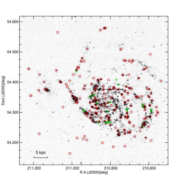
Figure 1: Location of H ii regions of final 188 samples on the narrow-band H$\alpha$ image of M101 observed with KPNO Schmidt telescope (Hoopes et al., 2001). Two symbols represent spectra from two telescop: red circles from MMT and green diamonds from NAOC. The green cross marks the center of the galaxy.

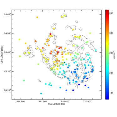
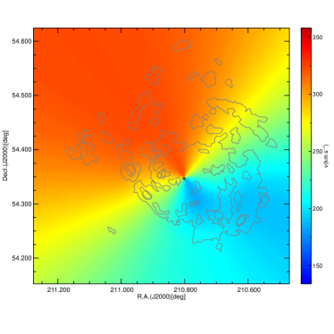
Figure 2: Velocity field of M101. Left: the line of sight velocities of H ii regions; Right: modeled velocity map using the method from Krajnović et al. (2006). Contours show the shape of M101 in H$\alpha$ image, and the center of the galaxy is marked with a black cross.

Finally we have 188 spectra in total (164 from MMT 6.5 m and 24 from NAOC 2.16 m). Locations of these H ii regions are shown in Figure 1 and their coordinates are listed in Table 1. Velocities are measured using the SAO xcsao package with IRAF (see Figure 2). We have carefully checked the velocities and corrected a few bad results manually. Spectra are corrected for Galactic reddening (Schlegel et al., 1998), and then shifted to rest frame for further measurements.

2.3 Spectral Fitting

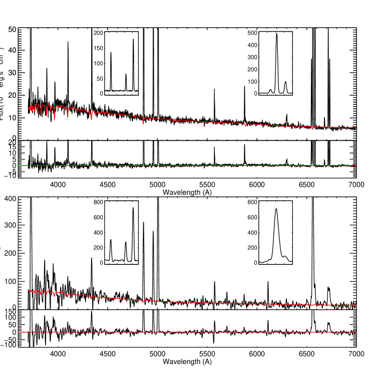
Figure 3: Typical spectrum of H ii regions in M101 observed by MMT (upper panel) and NAOC 2.16m (lower panel). Panels show the observed spectra (black line) and MF-ICA continuum fit (red line), and the two small insets of each spectrum zoom in several strong emission lines: H$\beta$+ [O iii]$\lambda\lambda$4959,5007, H$\alpha$+ [N ii]$\lambda\lambda$6548,6583.

To measure the emission lines of each individual spectra, the underlying stellar continuum must be subtracted. We perform a modeling of stellar continuum using advanced ICA algorithm, mean field approach to Bayesian independent component analysis (MF-ICA), which is comparatively precise and efficient (Højen-Sørensen et al., 2001, 2002). The MF-ICA approach extracts 12 independent components (ICs) from BC03 (Bruzual & Charlot, 2003). The 12 ICs contain full information of BC03 library and excellently recover the library, which spans a stellar age range from $1.0\times 10^{5}$ to $2.0\times 10^{10}$ yr, and an initial chemical composition metallicity from $0.0001$ to $0.1$. The star formation histories (SFHs) are parameterized in terms of an underlying continuous model superimposed with random bursts on it (Kauffmann et al., 2003). The intrinsic starlight reddening is modeled by the extinction law of Charlot & Fall (2000). The velocity dispersion is set to vary between 50 $\rm{km\,s^{-1}}$ and 450 $\rm{km\,s^{-1}}$. MF-ICA provides reliable modeling of stellar continuum and estimates physical parameters accurately with a large improvement in efficiency. More detailed informations about MF-ICA algorithm are described in Hu et al. (2016). Figure 3 shows two typical fitting results. For each spectrum, emission lines $\hbox{[O\,{\sc ii}]}\lambda 3727$, H$\beta$+ [O iii]$\lambda\lambda$4959,5007, H$\alpha$+ [N ii]$\lambda\lambda$6548,6583 and $\hbox{[S\,{\sc ii}]}\lambda\lambda 6717,6731$ are enlarged in four small panels below the spectrum.

2.4 Line Flux Measurement

After subtracting the stellar continuum, we perform the non-linear least-squares fit to emission lines using MPFIT package implemented in IDL (Markwardt, 2009). Each emission line is modeled with one Gaussian profile, and we constrain the ratios [N ii]$\lambda$6583/[N ii]$\lambda$6548 and [O iii]$\lambda$4959/[O iii]$\lambda$5007 to their theoretical values given by quantum mechanics. The emission line fluxes are measured by integration of the flux based on the fitted profiles.

The interstellar reddening is corrected by comparing the observed H$\alpha$/H$\beta$ Balmer decrement to the theoretical value, since intrinsic value of H$\alpha$/H$\beta$ is not very sensitive to the physical conditions of the gas. Assuming $\hbox{H$\alpha$}/\hbox{H$\beta$}=2.86$ and $R_{V}=3.1$ with Cardelli et al. (1989) extinction curve under the case-B recombination, the extinction in the V band is given by:

$$\centering A_{V}=6.77\log\frac{F(\hbox{H$\alpha$})/F(\hbox{H$\beta$})}{2.86}.\@add@centering$$ (1)

negative color excesses are all set to be zero. The reddening-corrected line flux measurements are listed in Table 1, with values normalized to H$\beta$ flux. All spectra have strong H$\alpha$ and H$\beta$ emission lines, and 14 of them have [O iii]$\lambda$4363 emission line.

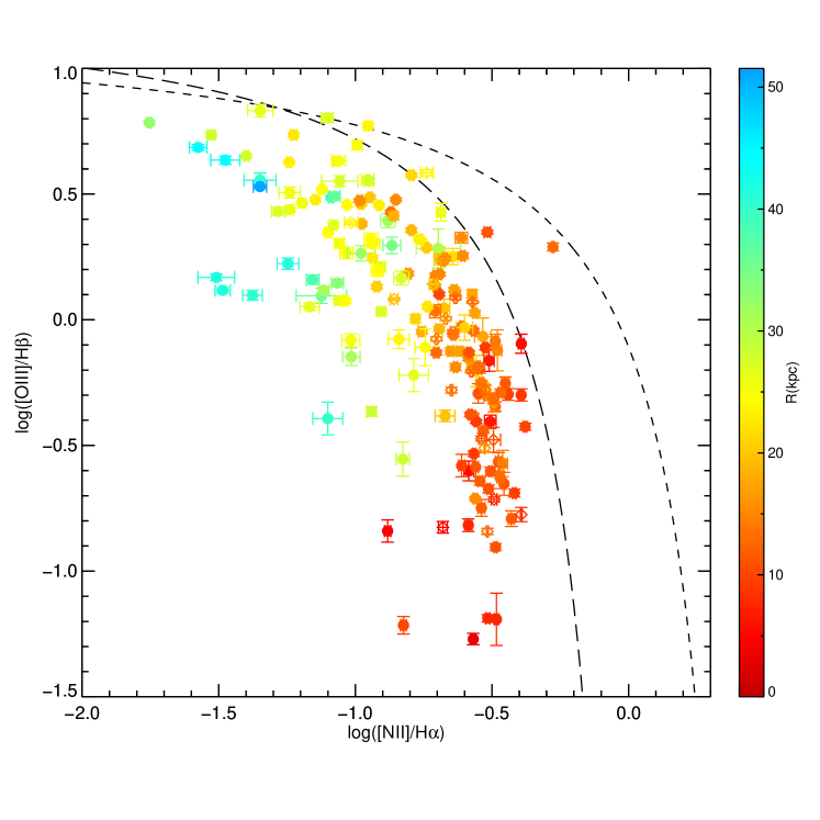
Figure 4: BPT diagram showing the excitation properties of our H ii regions. The boundaries are taken from Kewley et al. (2001, short-dashed line) and Kauffmann et al. (2003, long-dashed line). Filled points are from MMT and diamonds are from NAOC, and colors indicate the de-projected distance to the galaxy center. Almost all targets in our sample are located in the pure star forming region of the diagram with a clear profile against the de-projected distances to the galaxy center.

In Figure 4, we examine the excitation properties of our sample by plotting [O iii]$\lambda$5007/H$\beta$ versus [N ii]$\lambda$6583/H$\alpha$ diagnostic diagrams (BPT, Baldwin et al., 1981). The color-code indicates the de-projected distance to the galaxy center. We plot the boundaries between different photoionization sources (star-forming regions and active galactic nuclei) by Kewley et al. (2001) and Kauffmann et al. (2003). As shown in Figure 4, almost all targets in our sample are located in the pure star forming region with only 5 exceptions. Further, the H ii regions show a radially changing sequence on the BPT diagram: the inner regions have higher [N ii]$\lambda$6583/H$\alpha$ and lower [O iii]$\lambda$5007/H$\beta$ than outer regions, suggesting a negative gradient of metallicity. This is well consistent with the results from Sánchez et al. (2015), that the inner H ii regions of the galaxies appear to have higher [N ii]$\lambda$6583/H$\alpha$ and lower [O iii]$\lambda$5007/H$\beta$ than outer regions, using over 5000 H ii regions from 306 galaxies.

More detailed information will be discussed in section 3.3.

2.5 Oxygen Abundance determination

2.5.1 The direct method

The direct method to derive oxygen abundance is to measure the ratio of a higher excitation line to a lower excitation line, in which case $\hbox{[O\,{\sc iii}]}\lambda 4363/\hbox{[O\,{\sc iii}]}\lambda\lambda 4959,5007$ is the most commonly used. This ratio together with a model of two excitation zone structure for the H ii regions provides an estimation of the electron temperature of the gas, and then the electron temperatures are converted to oxygen abundances with corrections for unseen stage of ionization.

To calculate the total oxygen abundances, we make the usual assumption: $\rm{O/H}=(\rm{O}^{+}+\rm{O}^{2+})/\rm{H}^{+}$. Electron temperatures are derived based on the emission line intensity ratio $\hbox{[O\,{\sc iii}]}\lambda 4363/\hbox{[O\,{\sc iii}]}\lambda\lambda 4959,5007$, and electron densities ($n_{\rm{e}}$) are derived based on the intensity ratio $\hbox{[S\,{\sc ii}]}\lambda 6717/\hbox{[S\,{\sc ii}]}\lambda 6731$. Among the spectra of H ii regions, 14 of them have $\hbox{[O\,{\sc iii}]}\lambda 4363$ detections with well-defined line profiles and the S/Ns larger than 3. The electron temperatures of them for the $\rm{O}^{2+}$-emitting region ($T\hbox{[O\,{\sc iii}]}$) are derived with the PYNEB package (Luridiana et al., 2015). PYNEB is a python package for analyzing emission lines, which includes the Fortran code FIVEL (De Robertis et al., 1987) and the IRAF nebular package (Shaw & Dufour, 1995). We adopted the transition probabilities of Wiese et al. (1996) and Storey & Zeippen (2000) for $\rm{O}^{2+}$, Podobedova et al. (2009) for $\rm{S}^{+}$, the collision strengths of Aggarwal & Keenan (1999) for $\rm{O}^{2+}$, Tayal & Zatsarinny (2010) for $S^{+}$. Electron temperatures and electron densities are calculated simultaneously to obtain self-consistent estimates by PYNEB. Then the electron temperatures of [O ii] ($T\hbox{[O\,{\sc ii}]}$) are obtained with applying the relation from Garnett (1992): $T\hbox{[O\,{\sc ii}]}=0.7\times T\hbox{[O\,{\sc iii}]}+3000\rm{K}$. With giving $T\hbox{[O\,{\sc ii}]}$, $T\hbox{[O\,{\sc iii}]}$ and $n_{\rm{e}}$, metallicities are finally calculated from the line intensities of $\hbox{[O\,{\sc ii}]}\lambda 3727$ and $\hbox{[O\,{\sc iii}]}\lambda\lambda 4959,5007$ with PYNEB.

Errors are estimated with Monte Carlo algorithm by repeating the calculation 2000 times. In each calculation, the input flux of each emission line is generated from a Gaussian distribution with mean value equaling to measured emission line flux and standard deviation equaling to its error. We use the median value of 2000 results as the final value, and the half of $16\%-84\%$ range of this distribution as the corresponding error. The electron temperatures and densities are listed in Table 2.

Although the direct method is considered to be one of the most reliable methods to derive gas-phase oxygen abundances, the $\hbox{[O\,{\sc iii}]}\lambda 4363$ line is weak, especially in meta-rich environments. Since most of our H ii regions do not have $\hbox{[O\,{\sc iii}]}\lambda 4363$ detections, we applied two strong-line methods to determine the oxygen abundance.

2.5.2 O3N2 index

The O3N2 index, defined as $\rm{O3N2}=\log\{(\hbox{[O\,{\sc iii}]}\lambda 5007/\hbox{H$\beta$})/(\hbox{[N\,{\sc ii}]}\lambda 6583/\hbox{H$\alpha$})\}$, is firstly introduced by Alloin et al. (1979). It is widely used to diagnose oxygen abundances in the literature. The four lines involved in the index are easily detected, and the close wavelength between the two pairs of lines make the index nearly free from extinction. By using 137 extragalactic H ii regions, Pettini & Pagel (2004) empirically calibrated the O3N2 vs oxygen abundance determined by $T_{e}$ method and photoionization models. More recently, Marino et al. (2013) provide a new calibration with $T_{e}$ based metallicities of 603 H ii regions, which is adopted here:

$$\centering 12+\log\rm{(O/H)}=8.533-0.214\times\rm{O3N2},\@add@centering$$ (2)

However, O3N2 calibrations do not consider the variations of ionization parameter ($q$), which may cause systematic errors. More will be discussed in the next subsection.

2.5.3 KK04 method

Kobulnicky & Kewley (2004, hereafter KK04) adopted the stellar evolution and photoionization from Kewley & Dopita (2002) to produce a modified $R_{23}$ calibration. $R_{23}$ index, defined as $R_{23}=(\hbox{[O\,{\sc ii}]}\lambda 3727+\hbox{[O\,{\sc iii}]}\lambda\lambda 4959,5007)/\hbox{H$\beta$}$, is sensitive to the ionization parameter of the gas, which is defined as the ratio between the number of hydrogen ionizing photons passing through a unit area per second and the hydrogen density of the gas. The ionization parameter is typically derived based on the line ratio $O_{32}=\hbox{[O\,{\sc iii}]}\lambda 5007/\hbox{[O\,{\sc ii}]}\lambda 3727$, and it is also sensitive to oxygen abundance, therefore KK04 applied an iterative process to derive a consistent ionization parameter and oxygen abundance. First we determined whether the H ii regions lie on the upper or lower $R_{23}$ branch with ratio $\rm{N2O2}=\hbox{[N\,{\sc ii}]}\lambda 6583/\hbox{[O\,{\sc ii}]}\lambda 3727$, then we calculated an initial ionization parameter by assuming a starting oxygen abundance 8.0 for lower branch and 9.0 for upper branch. The initial ionization parameter is used to calculate an initial oxygen abundance. These processes are iterated until oxygen abundance converges. Errors are generated with the same Monte Carlo algorithm used in direct $T_{e}$ method, i.e. repeating the calculation 2000 times.

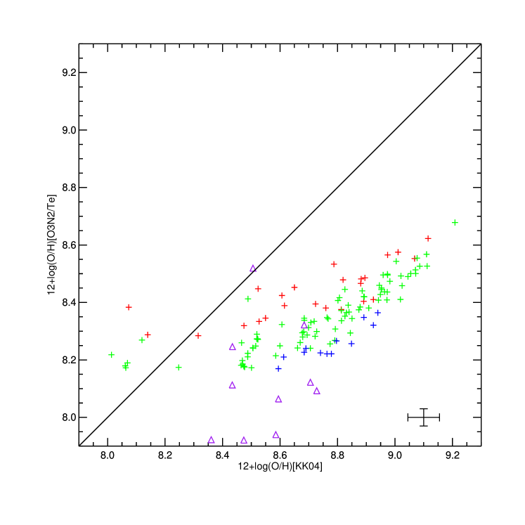
Figure 6: Comparation of the three abundance calibrations. Solid line is the y=x line. Triangle points represent direct $T_{e}$ calibration, and cross points represent O3N2 calibration. Different colors of cross ponits indicate different ionization parameter $q$: red, log($q$)<7.2; green, 7.2<log($q$) <7.7; blue, log($q$)>7.7. Error bar shows the typical error of the measurements.

The results of three calibrations, electron temperatures $T\hbox{[O\,{\sc iii}]}$, electron densities $n_{\rm{e}}$ and ionization parameter $q$ are listed in Table 2. To test the reliability of the oxygen abundance, we compare the three calibrations in Figure 6. In Figure 6 we plot O3N2 calibrations and $T_{e}$ calibrations vs KK04 calibrations, with different colors indicating different ionization parameter (see Figure 6 for details). As shown in this figure, good linear correlations are seen with systematic offsets as whole. O3N2 calibration is systematically $\sim$0.4 dex lower than KK04 calibration, and it flattens when KK04 calibration is lower than 8.5 due to the limited range of O3N2 index. $T_{e}$ calibrations agree well with O3N2 calibrations if we ignore the values near the lower limit of O3N2 calibration. The systematic biases of different methods are expected, which are investigated by Kewley & Ellison (2008) in detail. The systemic 0.4 dex bias could be caused by temperature fluctuations or gradients within high-metallicity H ii regions. In the presence of temperature fluctuations or gradients, [O iii] is emitted predominantly in high-temperature zones where O²⁺ is present only in small amounts. Thus the high electron temperatures estimated from the $\hbox{[O\,{\sc iii}]}\lambda 4363$ line do not reflect the true electron temperature in the H ii region, leading to a systematic lower estimation of metallicity by as much as 0.4 dex (Stasińska et al., 2002; Stasińska, 2005; Kewley & Ellison, 2008). Moreover, the scattering between O3N2 calibrations and KK04 calibrations is not random. It correlates with ionization parameter $q$: samples with lower log($q$) tend to have larger measured metallicity. Considering all the discussion above, we use KK04 calibrations in the following analysis.

3 Results

3.1 Velocity field

M101 is a giant and nearly face-on spiral galaxy (Sandage & Tammann, 1974; Bosma et al., 1981). The velocity field of M101 have been studied based on the kinematics of HI gas (Bosma et al., 1981) and H$\alpha$-data (Comte et al., 1979). In this paper, the H ii regions cover a wide range of regions on M101, which enables us to acquire the velocity map for M101. The left panel of Figure 2 shows the line of sight velocities of H ii regions in M101, which are good tracers of gas movements. The velocities are measured using the SAO xcsao package with IRAF.

As seen in this panel, a rotating disk is clearly shown. We then apply the harmonic decomposition method (Krajnović et al., 2006) to model the velocity field. This method has been widely used to analyze the gas and stellar kinematics in both late-type (Franx et al., 1994; Wong et al., 2004) and early-type galaxies (Emsellem et al., 2007; Krajnović et al., 2008). This method is able to decompose the line of sight velocity map into a series of Fourier components, which are kinematic components with different azimuthal symmetry. In this work, we broadly expand the Fourier terms to the third order:

$$V(a,\psi)=A_{0}(a)+\sum_{n=1}^{3}A_{n}(a)\sin{n\psi}+B_{n}(a)\cos(n\psi)$$ (3)

where $\psi$ is the eccentric anomaly, and $a$ is the length of the semimajor axis of the elliptical ring. Using this model, we obtained the kinematic position angle of 36 degree, the inclination of 26 degree, the systemic velocity of 242 km/s and the line of sight rotation velocity of 71 km/s, corresponding to a maximum rotation velocity of 168 km/s. These values agree well with the previous modeling of velocity field from Comte et al. (1979), who found the position angle of 35 degree, the inclination of 27 degree and the systemic velocity of 238 km/s. However, the inclination measured in this work is slightly larger than the result from Bosma et al. (1981), who found a inclination of 18 degree based on the HI velocity map. This discrepancy may due to the larger HI disks than optical disk and interactions with close companions in outskirts (Bosma et al., 1981; Waller et al., 1997; Mihos et al., 2012). The modeled velocity map is shown in the right panel of Figure 2 with the same color-coding of the left panel.

3.2 Stellar population ages

The light-weighted mean stellar age is a good tracer to the star formation history. Low stellar age indicates the young stellar population and recent strong star formation activities in the galaxy, while high stellar age means old stellar populations with few recent star formation activities. The equivalent width (EW) of H$\alpha$ emission line is sensitive to the ratio of present to past star formation rate, therefore it is expected to be correlated with stellar age, with the higher values the younger populations.

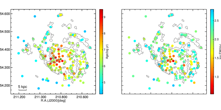
Figure 5: The two dimensional distrbution of stellar population age and EW(H$\alpha$). Contours show the shape of M101 in H$\alpha$ image, and center of the galaxy is marked with a black cross.

From the MF-ICA fits, we have estimated the stellar population age by computing light-weighed mean age of different stellar population components. The left panel of Figure 5 shows the two dimensional distribution of the mean stellar age. As shown in this figure, the stellar ages of the inner region are generally older than the outskirts in M101. We also present the EW(H$\alpha$) of each H ii region in the right panel of Figure 5. The results in both of panels are broadly consistent, with older stellar population in the inner regions and younger stellar population in outer regions. This negative stellar age gradient in M101 agrees with the “inside-out” disk growth scenario (Pérez et al., 2013; Bezanson et al., 2009; Tacchella et al., 2015).

We note that it appears to have a younger stellar population component at the very center of the bulge (see Figure 5). This is also discovered in Lin et al. (2013) by using SED modelings of resolved multi-band photometric images from ultraviolet and optical to infrared of M101. They found a resolved bar at the center of M101, and proposed that the bulge of M101 is a disk-like pseudobulge, likely induced by secular evolution of the small bar (Hawarden et al., 1986; Ho et al., 1997; Wang et al., 2012; Cole et al., 2014; Lin et al., 2017a).

3.3 Radial Abundance Gradient

The measurements of radial abundance gradient from H ii regions are firstly carried out by Searle (1971) and Smith (1975), after that series of works showed up (McCall et al., 1985; Kennicutt & Garnett, 1996; Bresolin, 2007; Lin et al., 2013; Sánchez et al., 2012, 2014, 2016b, 2017; Pilyugin et al., 2014; Belfiore et al., 2017).

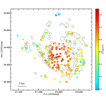
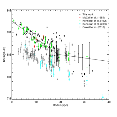
Figure 7: Left: distributions of metallicities of H ii regions in M101. Right: Radial metallicity gradient for H ii regions. Metallicities are determined from KKO4 calibration for this plot.

There are 173 out of 188 H ii regions whose oxygen abundances are computed by the KK04 calibration. The distribution of oxygen abundance (left panel) and its radial gradient (right panel) are presented in Figure 7. Some other works are also shown in different symbols. As the figure shows, the oxygen abundances from the KK04 calibration are 0.5 dex higher than Bresolin (2007) and Kennicutt et al. (2003), because their calibrations are based on the $T_{e}$ method. However, the metallicity gradients are consistent based on different calibrations and works. In addition, our result also shows a break in the gradient at around 18 kpc radius, so we use two linear least-squares fits:

$$\centering 12+\log(\rm{O/H})=9.24-0.0364\times\rm{R}\@add@centering$$ (4)

for R<18 kpc, and

$$\centering 12+\log(\rm{O/H})=8.64-0.00686\times\rm{R}\@add@centering$$ (5)

for R>18 kpc. The gradient of the inner regions is $-$0.0364 dex kpc^-1, which is slightly steeper than the results from Bresolin (2007), Li et al. (2013) and Pilyugin et al. (2014)($-$0.0278, $-$0.0268 and $-$0.0293 dex kpc^-1). However, the metallicity gradient becomes flat at the radius greater than 20 kpc. To compare with the characteristic gradient provided by Ho et al. (2015)($-$0.39$\pm$0.18 dex R${}_{25}^{-1}$), we convert the derived gradient to same scale. For inner regions, the gradient is $-$1.18$\pm$0.017 dex R${}_{25}^{-1}$, which is steeper than characteristic gradients. However, the gradient of the outer region is $-$0.221$\pm$0.038 dex R${}_{25}^{-1}$, which is flatter.

Rosales-Ortega et al. (2012) found that gas metallicity increases with stellar mass surface density, which plays a role in determining the mass-metallicity relation and radial metallicity gradients in spirals. This has been confirmed by several researches (e.g.,Sánchez et al. 2013, Barrera-Ballesteros et al. 2016). Chemical evolution models with most important parameters varying smoothly with radius can easily reproduce negative gradients, which show that the maxima of both neutral and molecular gas move from the center to outskirts through the disk as the galaxy evolves. Thus the star formation is strong in the central regions at early times and spread outward through disks as the gas is efficiently consumed. This shapes present galaxies with high metallicity, low specific star formation rate in the center and negative radial metallicity gradients that flatten with time. This is knew as the “inside-out” disk growth.

Several studies have found that metallicity gradients flatten to a constant value beyond the isophotal radii R₂₅ or 2R_e(Rosales-Ortega et al., 2011; Marino et al., 2012; Sánchez et al., 2012, 2014; López-Sánchez et al., 2015; Sánchez et al., 2016b). The mechanism of this gradient flattening is under debate. One possible mechanism is a slow radial dependence of the star formation efficiency across over a large galactocentric distances (Bresolin et al., 2012; Esteban et al., 2013). Cosmological simulations that introduce a balance between outflows and inflows with the intergalactic medium may also contribute to shaping the metal content (Oppenheimer & Davé, 2008; Oppenheimer et al., 2010; Davé et al., 2011, 2012). Interactions with satellite galaxies are suggested to enhance the metallicity in the outer regions of galaxies, which may also flatten the metallicity gradient (Bird et al., 2012; López-Sánchez et al., 2015). The real senario is likely to be the mixture of several mechanisms. We note that the turning point of the gradient in M101 is at $\sim$ 18 kpc, which is much smaller than R₂₅($\sim$ 31 kpc). An alternative explanation is proposed Lépine et al. (2011), that the break in the gradient is the “pumping out” effect of corotation, which produces gas flows in opposite directions on the two sides of the radius. The corotation radius of M101 is 16.7 kpc (Scarano & Lépine, 2013), which is very close to the break radius we find in this work. This suggests that the radial break of metallicity in M101 probably caused by the result of corotation.

There are 7 outliers far below the fit line with oxygen abundance lower than 8.2. These H ii regions are located to the east of M101. M101 is not the isolated galaxy, and two close companions (NGC5474 in the east and NGC5477 in the southeast) are found. Kewley et al. (2006) presented some evidence that galaxy pairs have systematically lower oxygen abundance than field galaxies, and mergers may also flatten the oxygen abundance gradient. More recently, Sánchez et al. (2014) found that the metallicity gradients are independent of morphology, incidence of bars, absolute magnitude and mass, and that the only clear correlation is between merger stage and metallicity gradient, where merger progresses flatten the slope of gradients (see also Torrey et al., 2012; Rich et al., 2012; Kewley et al., 2010; Rupke et al., 2010) . M101 might be interacting with NGC5474 and NGC 5477, as suggested by Waller et al. (1997); Mihos et al. (2012, 2013), who analyzed deep neutral hydrogen observation and deep optical images and concluded that M101 is in an ongoing interactions with lower mass companions. These interactions may dilute the oxygen abundance of these H ii regions in gas mixing processes, making the 7 outliers relatively meta-poor.

4 Summary

We have investigated the distributions of physical properties of H ii regions in nearby galaxy M101 using spectra obtained from the 6.5 m MMT telescope and the NAOC 2.16 m telescope during 2012 to 2014. We present the observations, data reductions, and measurements of emission lines. This is the largest spectroscopic sample of H ii regions in M101 by now.

We estimated the stellar population ages by fit the continuum with MF-ICA approach, and the stellar age profile shows an older stellar population in the inner regions and a younger in the outer regions. There is a younger component at the center of the galaxy, which indicates that a recent star formation occurred at the center. This might be caused by gas falling into the center due to the nonaxisymmetric gravity of the bar.

We calculated the electron temperatures $T\hbox{[O\,{\sc iii}]}$, electron densities $n_{e}$, and measured oxygen abundances with three methods. O3N2 calibrations are consistent with direct $T_{e}$ calibrations when ignore the limitation effect of O3N2 calibration, and both calibrations are systemically $\sim$0.4 dex lower than KK04 calibration, due to temperature fluctuations or gradients within high-metallicity H ii regions. O3N2 calibrations do not consider ionization parameters, which may cause systemic errors.

The oxygen abundance profile shows a negative gradient with a clear break at 20 kpc radius. The gradient is $-$0.0364 dex kpc^-1 in the inner region and $-$0.00686 dex kpc^-1 in the outer region. This is likely to be the mixture of several mechanisms, such as radial dependence of SFE over large a large galactocentric distances, a balance between outflows and inflows with the intergalactic medium and interactions with satellite galaxies. Since the break radius is comparable to the corotation radius (16.7 kpc), the break in the gradient could be the “pumping out” effect of corotation. If this is the case, gas flows play an important role in chemical evolutions of galaxies and should not be regarded as minor effects in evolution models. There are several H ii regions with oxygen abundance lower than 8.2, which locate far from major distribution, and we find they are all located in the east of M101, close to its companions, NGC5474 and NGC5477. These low metallicities may be the result of interactions with close companions.

Both stellar population age distribution and oxygen abundance gradient support the “inside-out” disk growth scenario: the early gas infall or collapse made the inner region more metal-rich and older, while the outer disk is enriched more slowly and younger. In order to learn more about the formation and evolution of nearby galaxies, we intend to combine the spectra of H ii regions with multi-wavelength photometry data (especially UV to IR) to investigate the nature of dispersions of IRX-$\beta$ relation. Due to the relatively simple star formation history and structure of H ii regions, it would be helpful to find a second parameter to reduce the scatter of IRX-$\beta$ relation. This will help us understand further in the interaction between dust and interstellar radiation field, as well as the formation and evolution of nearby galaxies.

Table 1: Coordinates and Dereddened Line Fluxes of H ii Regions in M101

ID	R.A.	Decl.	[O ii]	[Ne iii]	H$\delta$	H$\gamma$	[O iii]	[O iii]	[O iii]	[He i]	[O i]	[N ii]	H$\alpha$	[N ii]	[S ii]	[S ii]	H$\beta$
			$\lambda$3727	$\lambda$3869	$\lambda$4102	$\lambda$4340	$\lambda$4363	$\lambda$4959	$\lambda$5007	$\lambda$5876	$\lambda$6300	$\lambda$6548	$\lambda$6563	$\lambda$6583	$\lambda$6717	$\lambda$6731	$\lambda$4861
1	14:03:01.15	54:14:27.0	276.4	19.5	26.5	48.1	82.44	99.4	294.7	10.9	6.5	9.9	285.9	28.4	22.4	16.5	3611.51
			0.6	0.2	0.1	0.3	0.09	0.01	0.8	0.03	0.04	0.07	1.1	0.1	0.11	0.09	12.85
2	14:02:44.66	54:23:36.1	344.0	…	30.2	51.6	…	43.7	128.5	8.9	…	15.6	228.7	44.6	20.3	14.3	3478.57
			0.2	…	0.1	0.2	…	0.09	0.2	0.1	…	0.06	0.6	0.1	0.11	0.09	7.04
3	14:02:49.49	54:17:42.5	294.0	…	28.3	48.1	…	49.7	148.8	11.3	…	19.0	286.0	54.4	35.0	24.1	276.81
			1.9	…	0.6	0.4	…	0.05	1.3	0.4	…	0.01	2.4	0.4	0.66	0.32	2.37
4	14:02:20.22	54:23:12.8	434.4	…	40.7	46.6	…	51.2	152.7	11.9	…	11.1	286.9	31.9	41.5	28.1	131.22
			5.0	…	1.2	3.5	…	0.07	1.2	0.6	…	0.02	1.9	0.9	0.95	0.92	2.77
5	14:02:20.65	54:17:48.9	389.9	27.1	26.2	46.4	23.73	94.7	283.2	10.3	8.1	8.9	275.3	25.6	29.3	21.3	510.45
			2.4	0.9	0.5	0.4	0.35	0.01	1.2	0.3	0.2	0.05	1.3	0.2	0.07	0.18	6.79
6	14:03:45.54	54:13:53.3	482.9	43.4	…	77.8	…	103.1	304.0	…	…	4.8	236.9	13.6	16.9	16.6	174.60
			3.3	1.3	…	1.8	…	0.09	1.0	…	…	0.01	0.8	0.4	0.51	0.24	1.69
7	14:03:41.73	54:19: 4.0	374.0	21.2	36.3	56.6	…	94.3	275.3	9.6	3.9	10.5	286.0	29.9	14.1	11.2	23703.82
			0.1	0.01	0.02	0.1	…	0.04	0.2	0.01	0.1	0.02	0.4	0.02	0.03	0.02	24.11
8	14:03:34.05	54:18:37.1	174.1	12.1	30.0	50.7	…	86.3	256.0	12.6	2.6	11.9	252.0	34.0	9.1	7.5	18061.50
			0.3	0.1	0.2	0.3	…	0.03	0.6	0.1	0.1	0.01	1.2	0.1	0.04	0.05	63.28
9	14:02:46.64	54:14:49.7	334.0	40.9	29.5	56.4	7.29	125.1	374.6	8.6	12.7	15.9	286.0	45.5	44.6	32.2	354.90
			2.2	0.9	0.8	0.4	0.38	0.02	2.4	0.2	0.5	0.01	2.2	0.5	0.50	0.27	2.75
10	14:03:27.54	54:18:45.0	153.5	…	31.9	52.3	…	7.0	20.8	8.6	3.3	28.8	269.0	82.6	43.5	28.3	442.82
			1.2	…	0.5	0.5	…	0.01	0.4	0.2	0.2	0.01	0.9	0.5	0.51	0.25	1.80
11	14:02:29.51	54:16:14.1	295.0	15.8	25.6	46.4	…	92.9	275.6	10.9	6.6	10.7	251.7	30.7	26.3	18.0	1471.36
			0.8	0.2	0.3	0.4	…	0.01	0.5	0.1	0.2	0.02	1.0	0.2	0.12	0.15	6.10
12	14:02:46.97	54:16:56.1	280.2	…	33.0	36.7	…	21.6	64.7	…	8.8	26.1	286.0	74.9	40.1	23.5	110.45
			4.0	…	2.1	1.3	…	0.02	1.9	…	0.7	0.01	3.0	0.7	0.95	0.62	1.72
13	14:03:12.28	54:17:54.2	222.8	…	14.0	49.0	…	21.2	63.6	11.6	…	27.8	279.3	79.8	44.1	30.3	164.75
			2.8	…	0.8	2.2	…	0.01	1.6	0.6	…	0.03	1.6	0.8	1.06	0.22	2.31
14	14:02:20.29	54:20: 1.4	275.7	21.6	28.6	47.3	…	100.1	300.4	11.0	6.2	7.0	286.2	20.2	18.6	13.5	576.54
			2.5	0.6	0.8	0.8	…	0.02	1.7	0.2	0.2	0.04	2.1	0.2	0.17	0.22	5.98
15	14:02:12.15	54:19:37.9	175.2	78.7	…	…	…	227.3	681.8	…	…	…	237.9	…	…	…	34.70
			11.6	6.4	…	…	…	0.04	6.5	…	…	…	2.3	…	…	…	1.69

Note. —  Line fluxes are normalized to H$\beta$line, after correcting for reddening. H$\beta$$\lambda$4861 is the measured H$\beta$ flux in units of $\times 10^{-17}$erg s^-1 cm^-2, corrected for extinction.

Table 2: Gas Conditions and Oxygen Abundance Measurements

ID	$T\hbox{[O\,{\sc iii}]}$	$n_{e}$	$\log q$	$12\,+\,{\rm log(O/H)}$
	(K)	(cm -3)	$(\log$ cm s${}^{-1})$	O3N2	KK04	$T_{e}$
1	10120 $\pm$ 1134	76 $\pm$ 12	7.77 $\pm$ 0.153	8.27 $\pm$ 0.023	8.68 $\pm$ 0.009	8.32 $\pm$ 0.933
2	…	29 $\pm$ 7	7.47 $\pm$ 0.019	8.46 $\pm$ 0.013	8.83 $\pm$ 0.002	…
3	…	…	7.60 $\pm$ 0.654	8.45 $\pm$ 0.070	8.85 $\pm$ 0.009	…
4	…	…	7.37 $\pm$ 1.145	8.37 $\pm$ 0.096	8.68 $\pm$ 0.012	…
5	13696 $\pm$ 1415	62 $\pm$ 11	7.57 $\pm$ 0.388	8.25 $\pm$ 0.036	8.59 $\pm$ 0.017	7.94 $\pm$ 0.820
6	…	539 $\pm$ 30	7.55 $\pm$ 3.646	8.17 $\pm$ 0.036	8.63 $\pm$ 0.009	…
7	…	170 $\pm$ 29	7.58 $\pm$ 0.056	8.31 $\pm$ 0.006	8.60 $\pm$ 0.002	…
8	…	215 $\pm$ 37	8.05 $\pm$ 0.394	8.32 $\pm$ 0.021	8.85 $\pm$ 0.004	…
9	9519 $\pm$ 2096	53 $\pm$ 20	7.68 $\pm$ 0.343	8.29 $\pm$ 0.057	8.51 $\pm$ 0.020	8.52 $\pm$ 1.876
10	…	…	7.33 $\pm$ 0.773	8.78 $\pm$ 0.078	9.11 $\pm$ 0.003	…
11	…	…	7.72 $\pm$ 0.283	8.29 $\pm$ 0.017	8.69 $\pm$ 0.008	…
12	…	…	7.39 $\pm$ 1.443	8.61 $\pm$ 0.165	8.95 $\pm$ 0.010	…
13	…	…	7.53 $\pm$ 1.244	8.62 $\pm$ 0.147	9.02 $\pm$ 0.010	…
14	…	62 $\pm$ 15	7.65 $\pm$ 0.572	8.21 $\pm$ 0.050	8.47 $\pm$ 0.206	…
16	…	59 $\pm$ 16	…	…	9.16 $\pm$ 0.004	…
17	…	…	7.96 $\pm$ 1.300	8.45 $\pm$ 0.039	8.89 $\pm$ 0.008	…
18	15259 $\pm$ 764	69 $\pm$ 27	7.65 $\pm$ 0.539	8.20 $\pm$ 0.043	8.46 $\pm$ 0.133	7.79 $\pm$ 0.390
19	…	20 $\pm$ 7	…	…	9.03 $\pm$ 0.004	…
20	…	…	7.44 $\pm$ 2.586	8.57 $\pm$ 0.114	8.95 $\pm$ 0.018	…
21	…	113 $\pm$ 34	7.48 $\pm$ 0.211	8.68 $\pm$ 0.023	9.07 $\pm$ 0.002	…
22	…	…	7.76 $\pm$ 2.431	8.25 $\pm$ 0.088	8.61 $\pm$ 0.018	…
23	…	164 $\pm$ 35	…	…	……	…
24	…	25 $\pm$ 9	7.42 $\pm$ 0.569	8.59 $\pm$ 0.115	8.96 $\pm$ 0.011	…
25	…	…	7.69 $\pm$ 2.493	8.55 $\pm$ 0.101	9.02 $\pm$ 0.006	…
26	…	55 $\pm$ 12	7.43 $\pm$ 0.433	8.44 $\pm$ 0.038	8.68 $\pm$ 0.010	…
27	…	…	…	…	8.86 $\pm$ 0.013	…
28	…	498 $\pm$ 22	7.42 $\pm$ 0.453	8.29 $\pm$ 0.089	8.66 $\pm$ 0.024	…
29	…	923 $\pm$ 83	7.39 $\pm$ 0.445	8.30 $\pm$ 0.255	8.51 $\pm$ 0.179	…
30	…	182 $\pm$ 15	7.56 $\pm$ 3.270	8.33 $\pm$ 0.144	8.79 $\pm$ 0.014	…

References

- Aggarwal & Keenan (1999) Aggarwal, K. M., & Keenan, F. P. 1999, ApJS, 123, 311
- Bacon et al. (2001) Bacon, R., Copin, Y., Monnet, G., et al. 2001, MNRAS, 326, 23
- Baldwin et al. (1981) Baldwin, J. A., Phillips, M. M., & Terlevich, R. 1981, PASP, 93, 5
- Barrera-Ballesteros et al. (2016) Barrera-Ballesteros, J. K., Heckman, T. M., Zhu, G. B., et al. 2016, MNRAS, 463, 2513
- Belfiore et al. (2017) Belfiore, F., Maiolino, R., Tremonti, C., et al. 2017, MNRAS, 469, 151
- Bertin & Arnouts (1996) Bertin, E., & Arnouts, S. 1996, A&AS, 117, 393
- Berg et al. (2013) Berg, D. A., Skillman, E. D., Garnett, D. R., et al. 2013, ApJ, 775, 128
- Bezanson et al. (2009) Bezanson, R., van Dokkum, P. G., Tal, T., et al. 2009, ApJ, 697, 1290
- Bird et al. (2012) Bird, J. C., Kazantzidis, S., & Weinberg, D. H. 2012, MNRAS, 420, 913
- Bosma et al. (1981) Bosma, A., Goss, W. M., & Allen, R. J. 1981, A&A, 93, 106
- Bresolin (2007) Bresolin, F. 2007, ApJ, 656, 186
- Bresolin (2011) Bresolin, F. 2011, ApJ, 730, 129
- Bresolin et al. (2012) Bresolin, F., Kennicutt, R. C., & Ryan-Weber, E. 2012, ApJ, 750, 122
- Bruzual & Charlot (2003) Bruzual, G., & Charlot, S. 2003, MNRAS, 344, 1000
- Bundy et al. (2015) Bundy, K., Bershady, M. A., Law, D. R., et al. 2015, ApJ, 798, 7
- Caldwell et al. (2009) Caldwell, N., Harding, P., Morrison, H., et al. 2009, AJ, 137, 94
- Cardelli et al. (1989) Cardelli, J. A., Clayton, G. C., & Mathis, J. S. 1989, ApJ, 345, 245
- Carollo et al. (2007) Carollo, C. M., Scarlata, C., Stiavelli, M., Wyse, R. F. G., & Mayer, L. 2007, ApJ, 658, 960
- Cavichia et al. (2014) Cavichia, O., Mollá, M., Costa, R. D. D., & Maciel, W. J. 2014, MNRAS, 437, 3688
- Cid Fernandes et al. (2005) Cid Fernandes, R., Mateus, A., Sodré, L., Stasińska, G., & Gomes, J. M. 2005, MNRAS, 358, 363
- Charlot & Fall (2000) Charlot, S., & Fall, S. M. 2000, ApJ, 539, 718
- Chiappini et al. (2001) Chiappini, C., Matteucci, F., & Romano, D. 2001, ApJ, 554, 1044
- Cole et al. (2014) Cole, D. R., Debattista, V. P., Erwin, P., Earp, S. W. F., & Roškar, R. 2014, MNRAS, 445, 3352
- Crockett et al. (2006) Crockett, N. R., Garnett, D. R., Massey, P., & Jacoby, G. 2006, ApJ, 637, 741
- Croxall et al. (2016) Croxall, K. V., Pogge, R. W., Berg, D. A., Skillman, E. D., & Moustakas, J. 2016, ApJ, 830, 4
- Comte et al. (1979) Comte, G., Monnet, G., & Rosado, M. 1979, A&A, 72, 73
- Cutri et al. (2003) Cutri, R. M., Skrutskie, M. F., van Dyk, S., et al. 2003, VizieR Online Data Catalog, 2246,
- Daddi et al. (2005) Daddi, E., Renzini, A., Pirzkal, N., et al. 2005, ApJ, 626, 680
- Dalcanton et al. (2004) Dalcanton, J. J., Yoachim, P., & Bernstein, R. A. 2004, ApJ, 608, 189
- Davé et al. (2011) Davé, R., Finlator, K., & Oppenheimer, B. D. 2011, MNRAS, 416, 1354
- Davé et al. (2012) Davé, R., Finlator, K., & Oppenheimer, B. D. 2012, MNRAS, 421, 98
- De Robertis et al. (1987) De Robertis, M. M., Dufour, R. J., & Hunt, R. W. 1987, JRASC, 81, 195
- Emsellem et al. (2007) Emsellem, E., Cappellari, M., Krajnović, D., et al. 2007, MNRAS, 379, 401
- Esteban et al. (2013) Esteban, C., Carigi, L., Copetti, M. V. F., et al. 2013, MNRAS, 433, 382
- Fabricant et al. (2005) Fabricant, D., Fata, R., Roll, J., et al. 2005, PASP, 117, 1411
- Fan et al. (2016) Fan, Z., Wang, H., Jiang, X., et al. 2016, PASP, 128, 5005
- Franx et al. (1994) Franx, M., van Gorkom, J. H., & de Zeeuw, T. 1994, ApJ, 436, 642
- Fu et al. (2009) Fu, J., Hou, J. L., Yin, J., & Chang, R. X. 2009, ApJ, 696, 668
- Ganda et al. (2007) Ganda, K., Peletier, R. F., McDermid, R. M., et al. 2007, MNRAS, 380, 506
- Garnett (1992) Garnett, D. R. 1992, AJ, 103, 1330
- Gordon et al. (2008) Gordon, K. D., Engelbracht, C. W., Rieke, G. H., et al. 2008, ApJ, 682, 336-354
- Hawarden et al. (1986) Hawarden, T. G., Mountain, C. M., Leggett, S. K., & Puxley, P. J. 1986, MNRAS, 221, 41
- Henry & Howard (1995) Henry, R. B. C., & Howard, J. W. 1995, ApJ, 438, 170
- Ho et al. (1997) Ho, L. C., Filippenko, A. V., & Sargent, W. L. W. 1997, ApJ, 487, 591
- Ho et al. (2015) Ho, I.-T., Kudritzki, R.-P., Kewley, L. J., et al. 2015, MNRAS, 448, 2030
- Hodge et al. (1990) Hodge, P. W., Gurwell, M., Goldader, J. D., & Kennicutt, R. C., Jr. 1990, ApJS, 73, 661
- Hoopes et al. (2001) Hoopes, C. G., Walterbos, R. A. M., & Bothun, G. D. 2001, ApJ, 559, 878
- Højen-Sørensen et al. (2001) Højen-Sørensen, P. A. D. F. R., Winther, O. & Hansen, L. K. 2001, Advances in Neural Information Processing Systems, Vol. 13, MIT Press, Cambridge, MA, 542
- Højen-Sørensen et al. (2002) Højen-Sørensen, P. A. D. F. R., Winther, O. & Hansen, L. K. 2002, Neural Comput, 14, 889
- Hu et al. (2016) Hu, N., Su, S.-S., & Kong, X. 2016, RAA, 16, 42
- Kauffmann et al. (2003) Kauffmann, G., Heckman, T. M., Tremonti, C., et al. 2003, MNRAS, 346, 1055
- Kewley et al. (2001) Kewley, L. J., Dopita, M. A., Sutherland, R. S., Heisler, C. A., & Trevena, J. 2001, ApJ, 556, 121
- Kewley & Dopita (2002) Kewley, L. J., & Dopita, M. A. 2002, ApJS, 142, 35
- Kewley et al. (2006) Kewley, L. J., Geller, M. J., & Barton, E. J. 2006, AJ, 131, 2004
- Kewley & Ellison (2008) Kewley, L. J., & Ellison, S. L. 2008, ApJ, 681, 1183
- Kewley et al. (2010) Kewley, L. J., Rupke, D., Zahid, H. J., Geller, M. J., & Barton, E. J. 2010, ApJ, 721, L48
- Kennicutt & Garnett (1996) Kennicutt, R. C., Jr., & Garnett, D. R. 1996, ApJ, 456, 504
- Kennicutt et al. (2003) Kennicutt, R. C., Jr., Bresolin, F., & Garnett, D. R. 2003, ApJ, 591, 801