Learning the Joint Representation of Heterogeneous Temporal Events
for Clinical Endpoint Prediction

Abstract

The availability of a large amount of electronic health records (EHR) provides huge opportunities to improve health care service by mining these data. One important application is clinical endpoint prediction, which aims to predict whether a disease, a symptom or an abnormal lab test will happen in the future according to patients’ history records. This paper develops deep learning techniques for clinical endpoint prediction, which are effective in many practical applications. However, the problem is very challenging since patients’ history records contain multiple heterogeneous temporal events such as lab tests, diagnosis, and drug administrations. The visiting patterns of different types of events vary significantly, and there exist complex nonlinear relationships between different events. In this paper, we propose a novel model for learning the joint representation of heterogeneous temporal events. The model adds a new gate to control the visiting rates of different events which effectively models the irregular patterns of different events and their nonlinear correlations. Experiment results with real-world clinical data on the tasks of predicting death and abnormal lab tests prove the effectiveness of our proposed approach over competitive baselines.

Introduction

The volume of electronic health records (EHR) is expanding at a staggering rate, providing a great opportunity for machine learning and data mining researchers to analyze these data so as to provide better health care service. An important application of machine learning in health care is predicting the clinical endpoints such as a disease, symptom, or laboratory abnormality based on patients’ historical records.

This paper develops effective deep learning techniques for clinical endpoint prediction since deep learning techniques have been proved effective for predictive analysis in a variety of applications such as image recognition (?), speech recognition (?), and natural language understanding (?). The goal of deep learning is to learn effective semantic representations of the high-dimensional data such as images, speeches and natural language. Therefore, our goal is to effectively represent patients’ historical records.

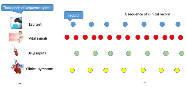
Figure 1: Heterogeneous Temporal Events. The sampling rates of different events vary significantly from each other. Different kinds of events are highly correlated.

However, the problem is challenging since patients’ historical records contain a variety of heterogeneous temporal events such as different lab tests, routine vital signals, diagnosis, and drug administrations (See Fig. 1 as an example). The visiting rates of different events vary significantly. For example, a patient may take a blood test every morning while take a temperature test every two hours. Besides, there is a high level of dependency among different kinds of events. For instance, some diagnosis are made according to the results of some lab tests. As a result, these heterogeneous temporal events yield heterogeneous event sequences consisting of thousands of correlated event types, the visiting rate of which varies significantly.

In the literature, learning representations of sequences are widely studied especially in the domain of speech recognition and natural language understanding. The state-of-the-art approaches for sequence modeling are recurrent neural networks (?) (RNNs) with the Long Short-term Memory (LSTM) units (?). RNNs are commonly used for modeling homogeneous sequences, but it is nontrivial to apply them for modeling heterogeneous event sequences. There are some recent works based on multi-task Gauss Process (MTGP) (?) for modeling the correlations between multiple sequences. However, the computational cost of MTGP is too expensive for EHR data since there are thousands of types of events. Therefore, we are seeking an approach that is able to: (1) effectively model the irregular visiting patterns of different events; (2) model the complex nonlinear relationships between different events; (3) scale up a large number of different types of events.

In this paper, we propose such an approach called Heterogeneous Event LSTM(HE-LSTM) for learning the joint representation of heterogeneous event sequences. Our approach is an extension of Phased LSTM (?), which was recently proposed and is used to model irregular event-based sequential data. Compared to the vanilla LSTM model, Phased LSTM (?) adds a new time gate, which is able to naturally integrate inputs from several sensors of arbitrary sampling rates. But Phased LSTM is not suitable for modeling the heterogeneous event sequence with thousands of event types in longitudinal EHR data. Our proposed model extends it by modeling correlated heterogeneous events with multi-scale sampling rates. Each event type and its attributes are embedded and fed into HE-LSTM. The HE-LSTM is equipped with an event gate controlled by the event type embeddings and the their timestamps. With the help of the event gates, the HE-LSTM can perfectly trace the temporal information of different event types in the long heterogeneous event sequence by asynchronously sample important and related events in the heterogeneous event sequence. Therefore, the representation of heterogeneous temporal events can be updated base on the dependency of the current input event and other events maintained in the HE-LSTM.

We conduct extensive experiments on real-world clinical data. Experiment results on the tasks of death prediction and abnormal lab test prediction prove that our proposed approach outperforms competitive baselines. Our proposed approach can be widely used in modeling data collected from sensors with arbitrary sampling rates, such as data collected from mobile sensors.

Our main contributions are:

$\bullet$ We formulate the clinical endpoint prediction task based on EHR data as a representation learning problem of heterogeneous temporal events consists of asynchronous clinical records from multiple sources.

$\bullet$ We propose a novel model called HE-LSTM for learning the representations of heterogeneous event sequence. The model effectively models the multi-scale sampling rates of different kinds of events and their temporal dependency.

$\bullet$ We conducted experiment on real-world clinical data on the tasks of death and abnormal lab tests. Promising results prove the effectiveness of our proposed approach over competitive baselines.

Related Works

Clinical Endpoint Prediction

There are plenty of works trying to solve the clinical endpoint prediction problem. However, many of these works only use a small subset of the whole EHR sequences in order to avoid dealing with the high-dimensional event types. Some works select a subset of the clinical events from the EHR data according to the expertise of physicians (?). For instance, Alaa only uses a set of 21 (temporal) physiological streams comprising a set of 11 vital signs and 10 lab test scores to predict ICU admission (?). Some techniques select 50 time series from the whole set of EHR data, and transformed the fixed-size subset into a new latent space using the hyper-parameters of multi-task GP(MTGP) models. They then calculate the similarity of patient’s records in the new hyper-parameter space (?). It is notable that manually selecting only a fraction of clinical sequences from original EHR data as the input brings out expert bias, thus these works seldom make full use of the important information of original data.

Most works ignore the content or value of clinical events, and only use the type information of clinical events to predict the endpoints (?). Specifically, some approaches train the semantic embeddings for different categories of clinical events for endpoint predictions (?).RETAIN uses two reversed recursive neural networks(RNN) generating attention variables of sequential ICD-9 code groups for the prediction tasks (?). There are some works using convolution neural network(CNN) to model irregular medical codes for future risk predictions (?). These works only exploit the type information of historical clinical events to make predictions, ignoring the fine-grained varying attributes of the events. Our work is to address the issue by utilizing the rich type information of clinical events as well as the content and values of the events.

Deep Learning Models for Sequential Data

Standard RNNs trained with stochastic gradient descent have difficulty learning long-term dependencies (i.e. spanning more than 10 time steps) encoded in the input sequences owing to the vanishing gradient (?). The problem has been addressed for example by using a specialized neuron structure in Long Short-Term Memory (LSTM) networks  (?) that maintains constant backward flow in the error signal.

In the Clockwork RNN (CW-RNN) (?), the hidden layer is partitioned into separate modules, each processing inputs at its own temporal granularity, making computations only at its prescribed clock rate. In this way, the fixed clock periods help to contain long-term dependencies.

Phased LSTM  (?)is a state-of-the-art RNN architecture for modeling event-based sequential data. It extends LSTM by adding the time gate. The gate has three phases: it rises from 0 to 1 in the first phase and drops from 1 to 0 in the second phase, which are active states. During the third phase, the model is in the inactive state. Updates to $\bm{c}_{t}$ and $\bm{h}_{t}$ are permitted only in the active state. The Phased LSTM network can achieve fast convergence in most experiments, owing to the fact that the auto-sampling on the long sequential data conducted by the time gate maintains derivative error in the longer back propagation.

However, these models only focus on learning long-term dependencies in homogeneous sequences, lacking the ability to capture the various and complex temporal dependencies in heterogeneous temporal events, which usually exist in EHR data.

Task Definition

Here are some notations and the definition of the task.

Heterogeneous Events Sequence

The heterogeneous event is defined as the triple $e_{i}=(type,value,time)$. $type$ is the category of event, $value$ is the attribute of the event, $type$ and $value$ of $e_{i}$ are logged at $time$. It is noteworthy that the attributes $value$s of different event types can be either numerical or categorical variable. For example, the attributes of a lab test, e.g.lactate blood test, is numerical while the attribute of the clinical status, e.g. ectopia type, is categorical variable(i.e. fusion beats, nodal bigeminy).

Heterogeneous events are merged in the ascending order of the record time into a triple sequence $\{e_{i}\}$. We denote the heterogeneous event sequence in a period of time $[T_{start},T_{end}]$ as $\{e_{i}\}_{T_{start}\leq e_{i}.t\leq T_{end}}$.

Clinical Endpoint Prediction Task

The clinical endpoint prediction task is formulated as follow: given a clinical heterogeneous event sequence $\{e_{i}\}_{T_{start}\leq e_{i}.t\leq T_{end}}$, and a binary label $\hat{y}$ for the target endpoint occurring at $T_{end}$ + $24$ hours, the objective is to predict what the target endpoint is in 24 hours using $\{e_{i}\}_{T_{start}\leq e_{i}.t\leq T_{end}}$.

In this paper, we aim to dynamically predict two endpoint outcomes base on the heterogeneous event sequence of patient data in EHR. In the first “death prediction dataset”, the endpoint outcome is death in either hospital or discharge to home. In the second “lab test result prediction dataset”, the endpoint outcome is either an abnormal result of the potassium lab test, or clinical stability.

Proposed Method

In this section, we introduce the technical details about our proposed model. The overall view of our model is illustrated in Figure 2.

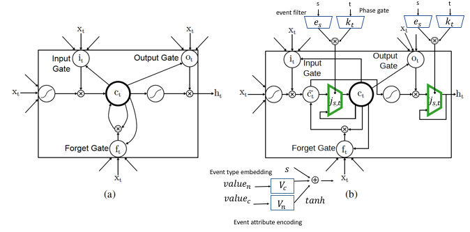
Figure 2: Model architecture. (a) Standard LSTM model. (b) HE-LSTM model, with event gate $\bm{j}_{t}$ consist of the event filter $\bm{e}_{s}$ and phase gate $\bm{k}_{t}$ separately controlled by the event type $\bm{s}$ and timestamp $t$. In the HE-LSTM formulation, each neural in the cell value $c_{t}$ and the hidden output $h_{t}$ can be updated during an “open” phase by only some certain types of events; otherwise, the previous values are maintained.

Event type embedding and attribute encoding

To help the HE-LSTM to trace temporal information of various kinds of events, we use “event type embedding” and “attribute encoding” to embed the type and attributes of the high dimensional events into compact continuous vectors, which can be trained end-to-end with the following HE-LSTM.

An event $e_{i}=(type,value,time)$ of the sequence will be embedded into three parts to feed the HE-LSTM for the endpoint prediction. The three input including embedding vector of event type $\bm{s}$, the event attribute encoding vector $\bm{x}$ and the scale variable time $t$.

The event type vector $\bm{s}$ carries the information of the event category of $\bm{e}_{i}$, and is constructed only by the one hot representation $\bm{type}$ of event type. Similar to word embedding (?), it will provide a low-dimension vector of the event type with semantic meaning in clinical field. The embedding lookup matrix $C_{type}\in\mathbb{R}^{N\times M}$, where $N$ is the embedding dimension and $M$ is the number of event types, is established for further training. The event type vector $\bm{s}$ is given by:

$$\bm{s}=C_{type}\times\bm{type}$$ (1)

The event attribute encoding vector $\bm{x}$ represents the combining information of both event type $\bm{type}$ and the attribute of the event $\bm{value}$, which is the main input of the following HE-LSTM. Each event has two kinds of attributes. One is categorical with the one hot representation $\bm{value_{c}}\in\{0,1\}^{C}$, where $C$ is the number of values of categorical attributes of all the event types. The other is numerical with the one hot representation $\bm{value_{n}}\in\mathbb{R}^{U}$, where $U$ is the number of all numerical attribute types of all the event types. Notice that the event attribute vector $\bm{value}=\left[\bm{value_{c}},\bm{value_{n}}\right]$.

Each value of categorical attributes is assigned with a vector from $V_{c}\in\mathbb{R}^{N\times C}$, where $N$ is the embedding dimension. As for numerical attributes, they are associated with a value encoding vector in $V_{n}\in\mathbb{R}^{N\times U}$, where $N$ is the embedding dimension.

The representing vector of a record $\bm{x}$ is mainly decided by its event type $\bm{s}$, however the event attributes also carries lots of information for modeling patients. The different values of the same event type, such as the abnormal label in a lab test event, can lead to distinct estimates for the patient’s future health status. The other important part of $\bm{x}$ is a disturbance from the numerical attribute values. For instance, the high numerical value of the lactate blood lab test event indicates potential health problem of the patient, while the low value does not offer much information. Finally, to combine the three parts of information, the attribute encoding vector $\bm{x}$ is given by:

$$\bm{x}=\bm{s}+V_{c}\times\bm{value_{c}}+\tanh(V_{n}\times\bm{value_{n}})$$ (2)

where $V_{c}$ and $V_{n}$ are parameters to learn.

Heterogeneous Event LSTM

Long short-term memory (LSTM) units (?) (Fig. 2(a)) is an important ingredient of modern deep RNN architectures. We first define their update equations in a commonly-used version in the following:

$$\bm{i}_{t} =\sigma(W_{ix}\bm{x}_{t}+W_{ih}\bm{h}_{t-1}+\bm{w}_{ic}\circ\bm{c}_{t-1}+\bm{b}_{i})$$ (3)

$$\bm{f}_{t} =\sigma(W_{fx}\bm{x}_{t}+W_{fh}\bm{h}_{t-1}+\bm{w}_{fc}\circ\bm{c}_{t-1}+\bm{b}_{f})$$ (4)

$$\bm{c}_{t} =\bm{f}_{t}\circ\bm{c}_{t-1}+\bm{i}_{t}\circ\tanh\big{(}W_{cx}\bm{x}_{t}+W_{ch}\bm{h}_{t-1}+\bm{b}_{c}\big{)}$$ (5)

$$\bm{o}_{t} =\sigma(W_{ox}\bm{x}_{t}+W_{oh}\bm{h}_{t-1}+\bm{w}_{oc}\circ\bm{c}_{t-1}+\bm{b}_{o})$$ (6)

$$\bm{h}_{t} =\bm{o}_{t}\circ\tanh\big{(}\bm{c}_{t}\big{)}$$ (7)

The main difference from classical RNNs is the use of the gating functions $\bm{i}_{t}$, $\bm{f}_{t}$, $\bm{o}_{t}$, which represent the input, forget, and output gate at time $t$ respectively. $\bm{c}_{t}$ is the cell activation vector, whereas $\bm{x}_{t}$ and $\bm{h}_{t}$ represent the input feature vector and the hidden output vector respectively. The gates use the typical sigmoid function $\sigma$ and $\tanh$ nonlinear function $\tanh$ with weight parameters $W_{ih}$, $W_{fh}$, $W_{oh}$, $W_{ix}$, $W_{fx}$, and $W_{ox}$, which connect the different inputs and gates with the memory cells and outputs, as well as biases $\bm{b}_{i}$, $\bm{b}_{f}$, and $\bm{b}_{o}$. The cell state $\bm{c}_{t}$ itself is updated with a fraction of the previous cell state that is controlled by $\bm{f}_{t}$, and a new input state created from the element-wise product, denoted by $\circ$, of $\bm{i}_{t}$ and the output of the cell state nonlinearity $\tanh$. Optional peephole (?) connection weights $\bm{w}_{ic}$, $\bm{w}_{fc}$, $\bm{w}_{oc}$ further influence the operation of the input, forget, and output gates.

HE-LSTM extends the LSTM model by adding a new event gate $\bm{j}_{s,t}$. The event gate has two factors — an event filter and a phase gate. The event filter only allows the information of a certain cluster of events to fuse into the corresponding memory cell, so that each cell will only trace a particular group of events. Collaborated with the phase gate, the event filter can help the network to maintain the temporal information of the different events in multi-scaled sampling rates. The dependency of the heterogeneous events will be easier to capture by the diverse and long memory of correlated events.

The opening and closing of this event gate is controlled by the event type embedding $\bm{s}$ and an independent rhythmic oscillation specified by the phase gate (?) with three parameters. And updates to the cell state $\bm{c}_{t}$ and $\bm{h}_{t}$ are permitted only when the gate is opened.

One factor of the event gate, the event filter $\bm{e}_{s}$, for each neuron is a feed forward network with a hidden layer of size $L$ with $\tanh$ activation function as following.

$$\bm{e}_{s} =\sigma(W_{em}\tanh\big{(}W_{ms}\bm{s}+\bm{b}_{m}\big{)}+\bm{b}_{e})$$ (8)

where $W_{em}\in\mathbb{R}^{H\times L}$, $W_{ms}\in\mathbb{R}^{L\times N}$, $\bm{b}_{e}\in\mathbb{R}^{H}$ and $\bm{b}_{m}\in\mathbb{R}^{L}$ are parameters to learn.

Considering the multi-scale sampling rates of the events, we extend the event filter $\bm{e}_{s}$ with a time factor proposed in phased LSTM (?) by three parameters: $t$, $r_{on}$ and $s$, where $t$ represents the real-time period of the gate, $s$ represents the phase shift and $r_{on}$ is the ratio of the open phase to the full period. $t$, $r_{on}$ and $s$ are learned by training. Therefore, $\bm{j}_{s,t}$ is formally defined as:

$$\phi_{t}=\frac{(t-s)\mod\tau}{\tau},k_{t}=\begin{cases}&\frac{2\phi_{t}}{r_{on}},\text{ if }\phi_{t}<\frac{1}{2}r_{on}\\ &2-\frac{2\phi_{t}}{r_{on}},\text{ if }\frac{1}{2}r_{on}<\phi_{t}<r_{on}\\ &\alpha\phi_{t},\text{ otherwise }\end{cases}$$ (9)

$$\bm{j}_{s,t}=\bm{e}_{s}\circ\bm{k}_{t}$$ (10)

Different from traditional RNNs for single sequential data and even sparser variants of RNNs  (?), updates in HE-LSTM can optionally be performed at irregularly sampled time points $t$ for different event types. This allows the RNNs to learn the multi-scale rhythm of related events and work with asynchronously sampled heterogeneous temporal event data. We use the shorthand notation $\bm{c}_{l}$ = $\bm{c}_{t_{l}}$ for cell states at time $t_{l}$ (analogously for other gates and units), and let $\bm{c}_{l-1}$ denote the state at the previous update time $t_{l-1}$. We can then rewrite the regular LSTM cell update equations for $\bm{c}_{l}$ and $\bm{h}_{l}$ (from Eq. 5 and Eq. 7), using proposed cell updates $\tilde{\bm{c}_{l}}$ and $\tilde{\bm{h}_{l}}$ mediated by the event gate $\bm{j}_{l}$ :

$$\bm{\tilde{}}{c_{l}} =\bm{f}_{l}\circ\bm{c}_{l-1}+\bm{i}_{l}\circ\tanh\big{(}W_{cx}\bm{x}_{l}+W_{ch}\bm{h}_{l-1}+\bm{b}_{c}\big{)}$$ (11)

$$\bm{c}_{l} =\bm{j}_{l}\circ\bm{\tilde{}}{c_{l}}+(1-\bm{j}_{l})\circ\bm{c}_{l-1}$$ (12)

$$\bm{\tilde{}}{h_{l}} =\bm{o}_{l}\circ\tanh\big{(}\bm{\tilde{}}{c_{l}}\big{)}$$ (13)

$$\bm{h}_{l} =\bm{j}_{l}\circ\bm{\tilde{}}{h_{l}}+(1-\bm{j}_{l})\circ\bm{h}_{l-1}$$ (14)

The HE-LSTM formulation ensures the flexible allocation and retain of information of each event clusters. Each neuron of the memory cell and hidden layer of HE-LSTM states can be updated only during the open periods of the event gate. In other words, only the information of a certain cluster of events’ records can flow into this certain neuron in its own phase. This is because the event filter $\bm{e}_{s}$, one of the factor of the event gate $\bm{j}_{s,t}$, can be seen as a binary classifier to chose the cluster of event types responsible for each neuron. Besides, the neuron maintains a perfect memory during its closed phase, i.e. $c_{l}=c_{l-\delta}$if $j_{l^{\prime}}=0$ for $t_{l}\leq l^{\prime}\leq t_{l-\delta}$. Thus, other neurons, tracing other events can directly use the information of this cluster of events even they are far away from each other in term of the sequence index. Because of this allocation mechanism, HE-LSTM can have much diverse and longer memory for modeling the dependency of multiple events.

We use a sigmoid layer to predict the true label $\hat{y_{t}}$ of the learned representation vector of sequence in the given decision times.

$$y_{t}=sigmoid(\bm{w}_{p}\bm{h}_{t}+b_{p})$$ (15)

where $\bm{w}_{p}\in\mathbb{R}^{N}$ and $b_{p}$ are parameters to learn.

We use cross-entropy to calculate the classification loss of the prediction $y_{t}$ and true label $\hat{y_{t}}$ of each sample as follows:

$$Loss(\hat{y_{t}},y_{t})=\frac{1}{N}\sum_{1\leq t\leq N}(\hat{y_{t}}\times\ln y_{t}+(1-\hat{y_{t}})\times\ln(1-y_{t}))$$ (16)

We can sum up the losses of all the samples in one mini-batch to get the total loss for back propagation.

Experiments

The source code of MIMIC-III EHR data preprocessing and the proposed model is available and can be found at https://github.com/pkusjh/HELSTM.

Data Description and Experimental Settings

We set up two data sets for evaluation of the models from one real clinical data source. MIMIC-III (?)(Medical Information Mart for Intensive Care III) is a large, freely-available database comprising de-identified health-related data relating to over forty thousand patients who stayed in critical care units of the Beth Israel Deaconess Medical Center between 2001 and 2012.

We extract all kinds of events from the MIMIC-III database to get the initial event type set(18192 kinds of events in total).The statistics of the event types with top frequency are listed in Table.1. By merging the heterogeneous events into triple sequence, we get a set of clinical event sequences. We drop out the sparse event types, whose frequency in total is less than 2500.

We extract episodes of patients, which are 24 hours before the occurrence time of each endpoint, from these event sequences as samples. And the upper bound of the record number of the samples is 1000. All the resulting sample events are labeled according to the target endpoint outcome in each task.

event sources	e.g. event types	# of types
lab test	HEMATOCRIT,	525
	WHITE BLOOD CELLS
vital signal	Heart Rate,	385
	Respiratory Rate
drug input	0.9% Normal Saline,	60
	Dextrose 5%
clinical symptom	Ectopy Type	2382
	Motor Response
procedure	electrocardiogram	19
	Invasive Ventilation
clinical output	Urine	17
	gastric retentive oral dosage

Table 1: Statistics of the event type

The statistics of the final clinical multiple sequences in two datasets are summarized in Table 2.

Dataset	# of samples	# of events	Avg timespan
death	24301(8%)	20290879	3d 15h 58m
lab test	784583(11%)	41006177	192d 22h 45m

Table 2: Statistics of the datasets(the percentage in the second column is the positive sample rate)

Each dataset is split into 3 parts with fixed proportions, namely training set(70%), validation set(10%) and evaluation set(20%). The data in validation set is used to select hyper-parameters of the proposed and comparing models and to conduct “early stop” while training, in which the samples may be different because of cross-validation. The evaluation set, the details of which is non-transparent for us in the process of training and parameter selection, will then be only used to calculate and report the evaluation metrics for comparison.

Methods	death		lab test
	AUC	AP	AUC	AP
Independent LSTM	0.8771 $\pm$ 0.0005	0.5573 $\pm$ 0.0006	0.7196 $\pm$ 0.0006	0.2969 $\pm$ 0.0008
Independent LSTM(shared weight)	0.8064 $\pm$ 0.0005	0.5301$\pm$ 0.0006	0.5308 $\pm$ 0.0005	0.1098 $\pm$ 0.0005
Phased LSTM	0.8474 $\pm$ 0.0005	0.4900 $\pm$ 0.0075	0.7722 $\pm$ 0.0007	0.3575 $\pm$ 0.0026
Clock-work RNN	0.8400 $\pm$ 0.0001	0.7181 $\pm$ 0.0003	0.6516 $\pm$ 0.0002	0.2208 $\pm$ 0.0003
RETAIN	0.8967 $\pm$ 0.0011	0.5808 $\pm$ 0.0114	0.7325 $\pm$ 0.0022	0.3096 $\pm$ 0.0052
LSTM + event embedding & attr encoding	0.9466 $\pm$ 0.0002	0.7445 $\pm$ 0.0007	0.7231 $\pm$ 0.0028	0.3021 $\pm$ 0.0014
HE-LSTM	0.9516 $\pm$ 0.0003	0.7687 $\pm$ 0.0011	0.7987 $\pm$ 0.0008	0.3914 $\pm$ 0.0013

Table 3: Performance of clinical endpoint prediction tasks

For all the results presented in this section, the networks, implemented with Theano (?),were trained with Adam  (?) set to default learning rate parameters.

Comparing Methods

We compare HE-LSTM to the following methods.

$\bullet$ Independent LSTM We use LSTM to model each homogeneous event independently and average the resulting representations into a logistic regression layer. Because the computational cost of thousands of independent LSTM exceed our tolerance, we select 25 important events as it was done in many works (?).

$\bullet$ Independent LSTM (shared weight) This model is the same as the previous one, except that the weights in each single LSTM is shared and all events are used as the input of the model.

$\bullet$ RETAIN RETAIN  (?) mimics physician practice by modeling the EHR data in a reverse time order, and a two-level RNN generating attention variables of sequential data can provides interpretation of the prediction.

$\bullet$ LSTM + event embedding & attr encoding We use the event embedding in the first part of proposed method section as the input of traditional LSTM. Logistic regression is applied to the top hidden layer.

$\bullet$ Clock-work RNN Clockwork RNN (?) described in related works section.

$\bullet$ Phased LSTM Phased LSTM (?) described in related works section.

Evaluating Metrics

All methods listed above can produce predict scores instead of binary labels, and the data for target prediction tasks are imbalanced labeled. So metrics for binary labels such as accuracy are not suitable for measuring the performance. Similar to the work (?; ?), we adopt the area under ROC curves (Receiver Operating Characteristic curves) and area under PRC (Precision-Recall curves) for evaluation. Both reflect the overall quality of predicted scores at each decision time, according to their true labels.

$\bullet$ the Area under ROC Curve(AUC) of comparing $y_{i}$ with the true label $\hat{y_{i}}$. AUC is robust to imbalanced positive/negative prediction labels, making it appropriate for evaluating the classification accuracy in the endpoint prediction prediction tasks.

$\bullet$ Average Precision(AP) Average precision (?) emphasizes ranking positive samples higher. It is the average of precisions computed at the point of each positive samples in the ranked sequence in ascending order of predict score:

$$AP=\frac{\sum_{r=1}^{N}(P(r)\times I(r))}{\mbox{number of positive samples}}$$ (17)

$$P(r)=\frac{|\{\mbox{positive samples of rank r or less}\}|}{r}$$ (18)

where r is the rank, N the total number of samples, $I()$ a index function on the positive sample of a given rank, and $P(r)$ precision at a given cut-off rank.

This metric is also referred to geometrically as the area under the Precision-Recall curve.

$\bullet$ Cross Entropy that measures the model loss on the test set. The loss can be calculated by Eq (16).

Quantitative Results

Methods		Phase gate	Event filter	Event gate
death prediction	AUC(1st epoch)	0.9301	0.9105	0.9370
	AUC	0.9471	0.9518	0.9516
	AP(1st epoch)	0.6856	0.6048	0.7094
	AP	0.7467	0.7679	0.7687
	Entropy(1st epoch)	0.1561	0.1835	0.1479
	Entropy	0.1369	0.1301	0.1297
abnormal lab test prediction	AUC(1st epoch)	0.7050	0.6747	0.7275
	AUC	0.7945	0.7559	0.7987
	AP(1st epoch)	0.2752	0.2403	0.2965
	AP	0.3875	0.3410	0.3914
	Entropy(1st epoch)	0.3373	0.3448	0.3298
	Entropy	0.3019	0.3178	0.3003

Table 4: Performance with different settings of the event gate

Table.3 shows the area under ROC and AP of different methods on death and lab test datasets respectively. From the results in Table.3, we draw the following conclusions:

Firstly, models considering the dependency of correlated events types outperform all the independent sequential models and the proposed HE-LSTM achieves the best performance. For example, on death prediction task, RETAIN, LSTM and HE-LSTM improve the AP of lab test prediction by around 4.3%, 2.4% and 32.1% respectively compared to the best of “independent LSTM” model without weight share of the parameters in each independent LSTMs. The similar results have been shown in other experiments and metrics. Furthermore, our model achieves the highest performance among these heterogeneous sequential models. For example, on lab test prediction task, HE-LSTM improves the AP by 26.2% and 29.4% compared to RETAIN and LSTM. Besides, the improvements on AUC are 9.0% and 10.4% respectively. We can draw the conclusion that the dependency information of correlated clinical temporal events is useful in endpoint prediction tasks and learning joint representations is more effective to model the temporal dependency of different events of EHR data compared to simple independent sequential models.

Secondly, compared to the densely updating recurrent neural networks, the RNNs adaptive to the sampling rate pattern of events make more improvement of the prediction performance. For example, clock-work RNN improve the AP of death prediction by 29.0% and 33.9% compared to the two kinds of independent LSTMs, while the improvements of AUC and AP are 7.0% and 20.7% for phased LSTM compared to the best of independent LSTMs in the lab test prediction task. We can draw the conclusion that multi-scaled sampling rate pattern of events is effective for endpoint prediction, which makes the model concentrate more on the important events in different phases other than treating all clinical events equally in the long sequence.

Thirdly, HE-LSTM achieves the best performance on all datasets and all evaluation metrics. HE-LSTM outperforms all sparsely updating recurrent neural networks and heterogeneous sequential models on each metrics of two datasets. Models solely utilizing multi-scale sampling pattern in event sequence or models straight-forwardly merging different type of events are not the best choice for clinical endpoint prediction in EHR data. Take the result of death prediction for example, HE-LSTM improves the AUC and AP by 12.4% and 7.0% respectively compared to the best of sparsely updating methods without the event type embedding and attribute encoding modules. The improvements of HE-LSTM compared to the heterogeneous sequential models without event gates are 3.4% and 30.3% in average in term of AUC and AP. We can draw the conclusion that the proposed HE-LSTM effectively improve the performance because of the joint effects of tracing the temporal dependency of heterogeneous events and adaptively fitting their multi-scaled sampling patterns.

Experiment on variations of the event gate

To evaluate the effect of the components in the event gate $\bm{j}_{s,t}$, we replace $\bm{j}_{s,t}$ in (Eq 10) with its factors, namely phase gate $\bm{k}_{t}$ and event filter $\bm{e}_{s}$ while remaining the other parts of the model identical. The results on two datasets are list in table 4, including AUC, AP and cross entropy on test data as well as the values of the three metrics when the first training epoch is finished.

The event filter mainly helps to improve the performance of clinical endpoint prediction tasks by modeling the dependency of heterogeneous events. Both the event gate and the event filter achieve good performance in all metrics and both datasets when the training is finished. For example, the event gate and the event filter improve the AUC of death prediction by 0.5% and 0.5% compared to the phase gate, while the improvements of AP are 2.8% and 2.9% and the improvements of entropy are 4.9% and 5.2%.

The phase gate helps to achieve a fast convergence in the early stage of training by fitting the multi-scaled sampling rates of different events. HE-LSTM and the model with only phase gate get much higher performance in all metrics and both datasets in the first epoch of training. Take results in lab test task for example, the phase gate and the event gate improve the AUC in first epoch by 4.6% and 7.9% compared to the event filter, while the improvements of AP are 14.5% and 23.3% and the improvements of entropy are 2.2% and 4.3%.

From these comparisons, we draw the conclusion that the event filter and the phase gate collaborates jointly in modeling the dependency in heterogeneous temporal events with the multi-scale sampling rates, which leads to the accurate and efficient performance on the clinical endpoint prediction task.

Experiment on varying length of multiple sequential data

To evaluate the ability to model the temporal dependency of heterogeneous temporal events of our proposed architect and the other baselines, we feed the trained models multiple events in test set with various length, in the range of 20 to 1000, as input. From figure 3, we can draw the following conclusions:

Firstly, temporal information is effective for endpoint prediction tasks. The performances of most models improve with the increase of the input sequence length. Especially, the performance increases sharply when the length of input sequence is less than 200.

Secondly, HE-LSTM is better at handling the dependency of heterogeneous temporal events than other models. When the input sequence is short, the performances of different models are similar. The reason lies in the fact that, for short sequence input, the combination of independent representations of a single event makes less difference from the joint representation of heterogeneous events in HE-LSTM. But when the input sequence get longer and longer, the performance of our model steadily increase from 0.7551 to 0.7687 in term of AP and from 0.9482 to 0.9516 in term of AUC. The performance of other models remained almost unchanged at almost 0.9465 of AUC and 0.7434 of AP.

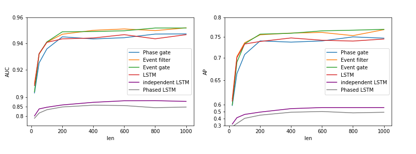
Figure 3: the performance on death prediction task with varying input length of the heterogeneous event sequence data

Different initial period

To explore the effect of the event filter in the event gate when modeling heterogeneous sequential EHR data, we compare the performance of the proposed HE-LSTM with the reduced HE-LSTM, of which the event filter factor in the event gate is removed. We use different initial periods of $\tau$ during training for death prediction task. The period was drawn uniformly in the exponential domain, comparing four sampling intervals $\exp(U(1,2))$, $\exp(U(2,3))$, $\exp(U(3,4))$, and $\exp(U(4,5))$ for each model. The results in Figure.4 show that the initialization of $\tau$ affects the performance of both models. But HE-LSTM is more robust to the initialization. For example, the improvements of HE-LSTM compared to the one without event filter are 4.1%, 4.1%, 2.8%and 6.6% on average. We can draw the conclusion that, with the help of event filter, the event gate can be more adaptive to multi-scale sampling rates of the events in the heterogeneous temporal sequence.

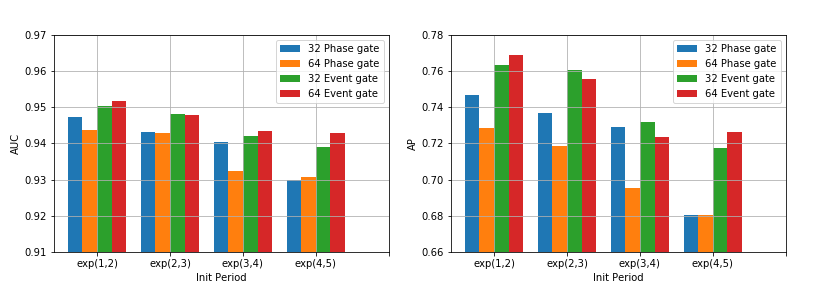
Figure 4: Different initial period

Conclusion

In this paper, we propose a novel HE-LSTM model to learn joint representations of heterogeneous temporal events for clinical endpoint prediction. Our model can adaptively fit the multi-scaled sampling rates of events in the heterogeneous event sequence. By tracing the temporal information of different kinds of events in the long sequence, the temporal dependency of different types of events can be captured in our learned representations. Experimental results with real-world clinical data on the tasks of predicting death and abnormal lab tests prove the effectiveness of our proposed approach over competitive baselines.

References

- [Alaa, Hu, and van der Schaar 2017] Alaa, A. M.; Hu, S.; and van der Schaar, M. 2017. Learning from clinical judgments: Semi-markov-modulated marked hawkes processes for risk prognosis. arXiv preprint arXiv:1705.05267.
- [Bergstra et al. 2010] Bergstra, J.; Breuleux, O.; Bastien, F.; Lamblin, P.; Pascanu, R.; Desjardins, G.; Turian, J.; Warde-Farley, D.; and Bengio, Y. 2010. Theano: A cpu and gpu math compiler in python. In Proc. 9th Python in Science Conf, 1–7.
- [Blunsom et al. 2017] Blunsom, P.; Cho, K.; Dyer, C.; and Schütze, H. 2017. From characters to understanding natural language (c2nlu): Robust end-to-end deep learning for nlp (dagstuhl seminar 17042). In Dagstuhl Reports, volume 7. Schloss Dagstuhl-Leibniz-Zentrum fuer Informatik.
- [Caballero Barajas and Akella 2015] Caballero Barajas, K. L., and Akella, R. 2015. Dynamically modeling patient’s health state from electronic medical records: A time series approach. In Proceedings of the 21th ACM SIGKDD International Conference on Knowledge Discovery and Data Mining, 69–78. ACM.
- [Choi et al. 2016] Choi, E.; Bahadori, M. T.; Sun, J.; Kulas, J.; Schuetz, A.; and Stewart, W. 2016. Retain: An interpretable predictive model for healthcare using reverse time attention mechanism. In Advances in Neural Information Processing Systems, 3504–3512.
- [Gers and Schmidhuber 2000] Gers, F. A., and Schmidhuber, J. 2000. Recurrent nets that time and count. In Neural Networks, 2000. IJCNN 2000, Proceedings of the IEEE-INNS-ENNS International Joint Conference on, volume 3, 189–194. IEEE.
- [Ghassemi et al. 2015] Ghassemi, M.; Pimentel, M. A.; Naumann, T.; Brennan, T.; Clifton, D. A.; Szolovits, P.; and Feng, M. 2015. A multivariate timeseries modeling approach to severity of illness assessment and forecasting in icu with sparse, heterogeneous clinical data. In Proceedings of the AAAI Conference on Artificial Intelligence. AAAI Conference on Artificial Intelligence, volume 2015, 446. NIH Public Access.
- [He et al. 2016] He, K.; Zhang, X.; Ren, S.; and Sun, J. 2016. Deep residual learning for image recognition. In Proceedings of the IEEE conference on computer vision and pattern recognition, 770–778.
- [Henriksson et al. 2015] Henriksson, A.; Zhao, J.; Bostrom, H.; and Dalianis, H. 2015. Modeling electronic health records in ensembles of semantic spaces for adverse drug event detection. In IEEE International Conference on Bioinformatics and Biomedicine, 343–350.
- [Hinton et al. 2012] Hinton, G.; Deng, L.; Yu, D.; Dahl, G. E.; Mohamed, A.-r.; Jaitly, N.; Senior, A.; Vanhoucke, V.; Nguyen, P.; Sainath, T. N.; et al. 2012. Deep neural networks for acoustic modeling in speech recognition: The shared views of four research groups. IEEE Signal Processing Magazine 29(6):82–97.
- [Hochreiter and Schmidhuber 1997] Hochreiter, S., and Schmidhuber, J. 1997. Long short-term memory. Neural computation 9(8):1735–1780.
- [Hochreiter et al. 2001] Hochreiter, S.; Bengio, Y.; Frasconi, P.; Schmidhuber, J.; et al. 2001. Gradient flow in recurrent nets: the difficulty of learning long-term dependencies.
- [Johnson et al. 2016] Johnson, A. E.; Pollard, T. J.; Shen, L.; Lehman, L.-w. H.; Feng, M.; Ghassemi, M.; Moody, B.; Szolovits, P.; Celi, L. A.; and Mark, R. G. 2016. Mimic-iii, a freely accessible critical care database. Scientific data 3.
- [Kingma and Ba 2014] Kingma, D., and Ba, J. 2014. Adam: A method for stochastic optimization. Computer Science.
- [Koutnik et al. 2014] Koutnik, J.; Greff, K.; Gomez, F.; and Schmidhuber, J. 2014. A clockwork rnn. In International Conference on Machine Learning, 1863–1871.
- [Liu et al. 2015] Liu, C.; Wang, F.; Hu, J.; and Xiong, H. 2015. Temporal phenotyping from longitudinal electronic health records: A graph based framework. In ACM SIGKDD International Conference on Knowledge Discovery and Data Mining, 705–714.
- [Mikolov et al. 2010] Mikolov, T.; Karafiát, M.; Burget, L.; Cernockỳ, J.; and Khudanpur, S. 2010. Recurrent neural network based language model. In Interspeech, volume 2, 3.
- [Mikolov et al. 2013] Mikolov, T.; Sutskever, I.; Chen, K.; Corrado, G. S.; and Dean, J. 2013. Distributed representations of words and phrases and their compositionality. In Advances in neural information processing systems, 3111–3119.
- [Neil, Pfeiffer, and Liu 2016] Neil, D.; Pfeiffer, M.; and Liu, S.-C. 2016. Phased lstm: Accelerating recurrent network training for long or event-based sequences. In Advances in Neural Information Processing Systems, 3882–3890.
- [Nguyen et al. 2016] Nguyen, P.; Tran, T.; Wickramasinghe, N.; and Venkatesh, S. 2016. Deepr: A convolutional net for medical records. IEEE Journal of Biomedical and Health Informatics.
- [Turpin and Scholer 2006] Turpin, A., and Scholer, F. 2006. User performance versus precision measures for simple search tasks. In Proceedings of the 29th annual international ACM SIGIR conference on Research and development in information retrieval, 11–18. ACM.