Learning Monocular 3D Human Pose Estimation from Multi-view Images

Abstract

Accurate 3D human pose estimation from single images is possible with sophisticated deep-net architectures that have been trained on very large datasets. However, this still leaves open the problem of capturing motions for which no such database exists. Manual annotation is tedious, slow, and error-prone. In this paper, we propose to replace most of the annotations by the use of multiple views, at training time only. Specifically, we train the system to predict the same pose in all views. Such a consistency constraint is necessary but not sufficient to predict accurate poses. We therefore complement it with a supervised loss aiming to predict the correct pose in a small set of labeled images, and with a regularization term that penalizes drift from initial predictions. Furthermore, we propose a method to estimate camera pose jointly with human pose, which lets us utilize multi-view footage where calibration is difficult, e.g., for pan-tilt or moving handheld cameras. We demonstrate the effectiveness of our approach on established benchmarks, as well as on a new Ski dataset with rotating cameras and expert ski motion, for which annotations are truly hard to obtain.

1 Introduction

With the advent of Deep Learning, the effectiveness of monocular 3D human pose estimation algorithms has greatly improved. This is especially true when capturing human motions for which there is enough annotated data to properly train the deep nets. Walking and upright poses are prime examples of this, and state-of-the-art algorithms [18, 27, 20, 15, 17] now deliver impressive real-time results in uncontrolled environments. However, this is not yet the case for more unusual motions for which the training data is harder to obtain, such as sports. Skiing is a good example of this, because pose estimation is crucial to biomechanical and performance analysis, and data cannot easily be acquired in a laboratory.

The brute-force approach to tackle such unusual motions would be to annotate video data. However, achieving high accuracy would require a great deal of annotation, which is tedious, slow, and error-prone. As illustrated by Fig. 1, we therefore propose to replace most of the annotations by the use of multiple views, at training time only. Specifically, we use them to provide weak supervision and force the system to predict the same pose in all views.

Figure 1: Multi-view constraints as weak supervision. Our approach lets us effectively train a deep network to predict 3D pose for actions where only little annotated data is available. This is the case for skiing, which cannot be captured in a laboratory.

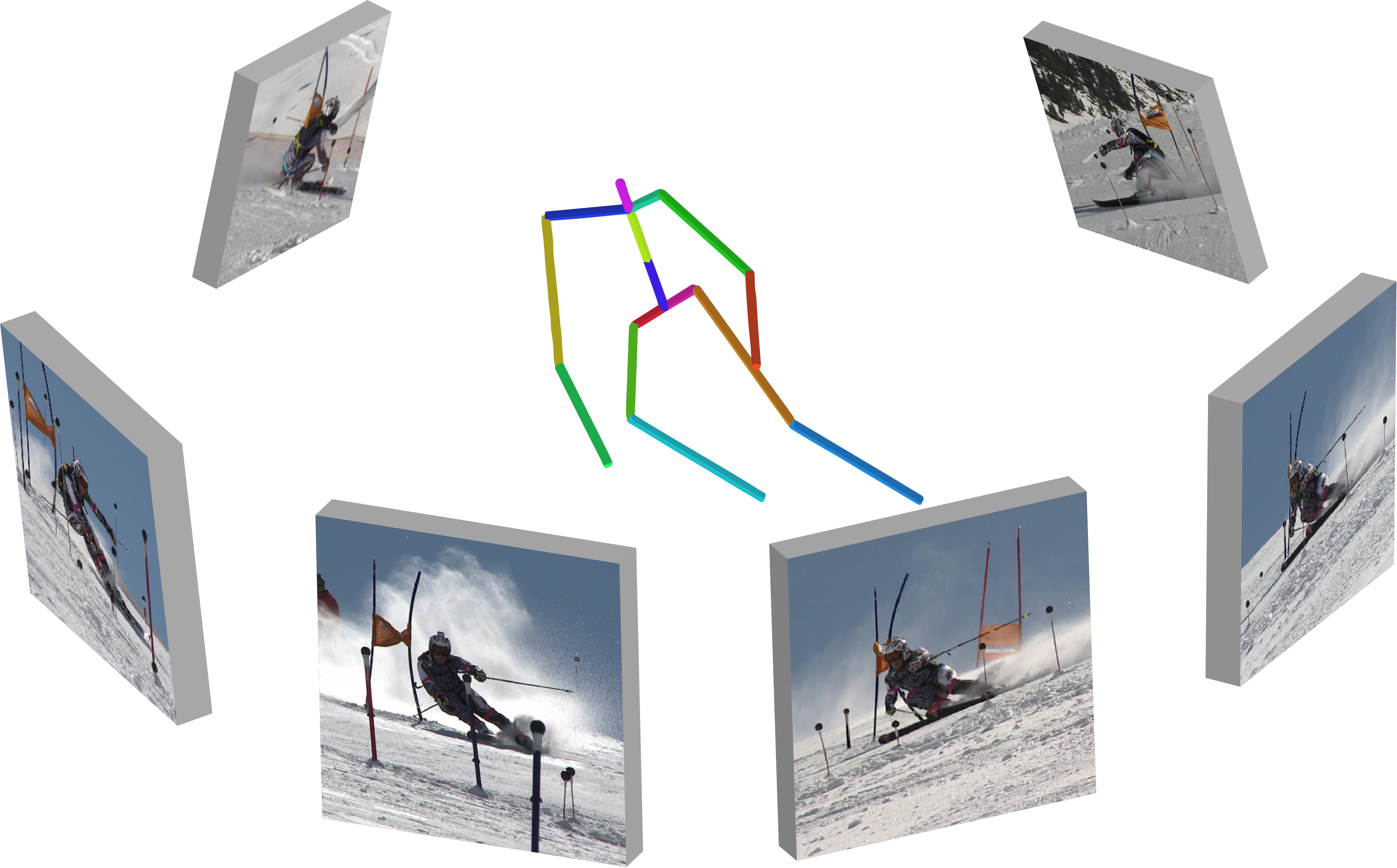
While such view consistency constraints increase accuracy, they are unfortunately not sufficient. For example, the network can learn to always predict the same pose, independently of the input image. To prevent this, we use a small set of images with ground-truth poses, which serve a dual purpose. First, they provide strong supervision during training. Second, they let us regularize the multi-view predictions by encouraging them to remain close to the predictions of a network trained with the scarce supervised data only.

In addition, we propose to use a normalized pose distance to evaluate all losses involving poses. It disentangles pose from scale, and we found it to be key to maintain accuracy when the annotated data is scarce.

Our experiments demonstrate the effectiveness of our weakly-supervised multi-view training strategy on several datasets, including standard 3D pose estimation benchmarks and competitive alpine skiing scenarios, in which annotated data is genuinely hard to obtain. Not only does our approach drastically cut the need for annotated data, but it also increases the robustness of our algorithm to viewpoint and scale changes.

2 Related work

Algorithms for 3D human pose estimation from single images [18, 27, 20, 15, 17, 23, 19, 31, 26, 25] have now matured to the point where they can operate in real-time and in the wild. They typically rely on sophisticated deep-net architectures that have been trained using very large datasets. However, dealing with motions for which no such database exists remains an open problem. In this section, we discuss the recent techniques that tackle this aspect.

Image Annotation.

An obvious approach is to create the required datasets, which is by no means easy and has become a research topic in itself. In a controlled studio environment, marker-suits [9] and marker-less motion capture systems [16, 11, 19] can be used to estimate the pose automatically. While effective for a subset of human activities, these methods do not generalize well to in-field scenarios in which videos must be annotated manually or using semi-automated tools [12]. However, even with such tools, the annotation process remains costly, labor-intensive and error-prone at large scales.

Data Augmentation.

An attractive alternative is to augment a small labeled dataset with synthetically generated images. This was done in [16, 21] by replacing the studio background and human appearance of existing datasets with more natural textures, and in [22] by generating diverse images via image mosaicing. Several authors have proposed to leverage recent advances in computer graphics and human rendering [14] to rely on fully-synthetic images [1, 29]. However, the limited diversity of appearance and motion that such simulation tools can provide, along with their not yet perfect realism, limits both the generality and the accuracy of networks trained using only synthetic images.

Weak supervision.

In this paper, this is the approach we focus on by introducing a weakly-supervised multi-view training method. It is related in spirit but different in both task and methodology to the method on geometric supervision of monocular depth estimation from stereo views of Garg et al. [6], the multi-view visual hull constraint used for reconstruction of static objects by Yan et al. [30] , and the differentiable ray-potential view-consistency used by Tulsiani et al. [28] . Weak supervision has been explored for pose estimation purposes in [31], which involves complementing fully-annotated data with 2D pose annotations. Furthermore, Simon et al. [24] iteratively improve a 2D pose detector through view consistency in a massive multi-view studio, using RANSAC and manual intervention to remove outliers. While effective for imposing reprojection constraints during training, these methods still require extensive manual 2D annotation in the images featuring the target motions and knowledge of the external camera matrix. By contrast, the only manual intervention our approach requires is to supply the camera intrinsic parameters, which are either provided by the manufacturer or can be estimated using standard tools.

Figure 2: Labeled and unlabeled examples. The loss $S(\theta,\mathcal{L})$ acts on the images (a) with associated poses (b), whereas the view consistency loss $M(\theta,\mathcal{U})$ exploits unlabeled images of different skiers that are taken at the same time (c). In (c) each column depicts the same camera and each row the same time $t$.

3 Approach

Our goal is to leverage multi-view images, for which the true 3D human pose is unknown, to train a deep network to predict 3D pose from a single image. To this end, we train our network using a novel loss function that adds view-consistency terms to a standard supervised loss evaluated on a small amount of labeled data and a regularization term that penalizes drift from initial pose predictions. This formulation enables us to use unlabeled multi-view footage by estimating jointly the body pose in a person-centered coordinate system and the rotation of that coordinate system with respect to the cameras.

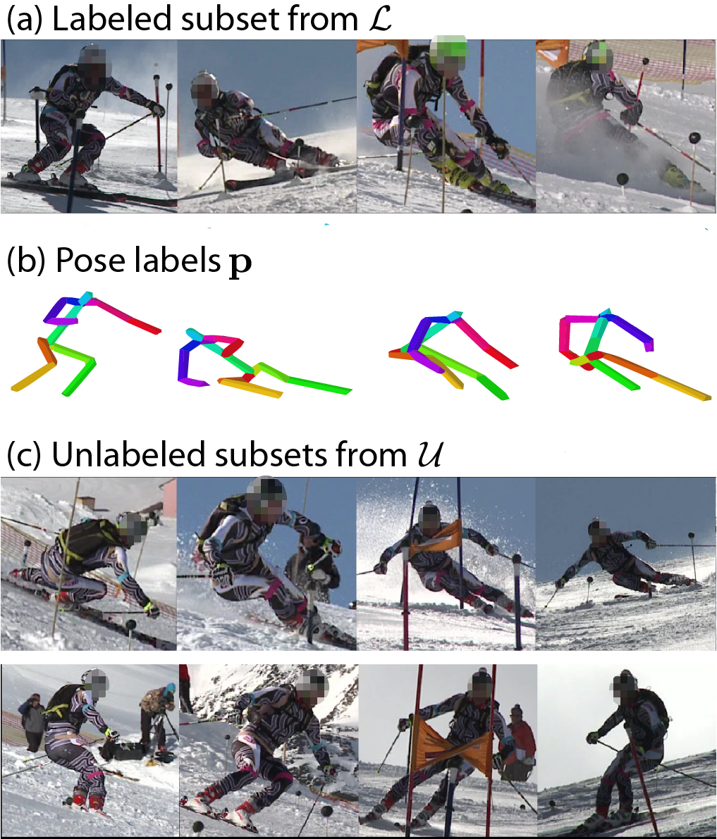
Formally, let $f_{\theta}$ denote the mapping, with parameters $\theta$, encoded by a CNN taking a monocular image $\mathbf{I}\in\mathbb{R}^{w\times h\times 3}$ as input and producing a 3D human pose $\mathbf{p}=f_{\theta}(\mathbf{I})\in\mathbb{R}^{3\times N_{J}}$ as output, where $N_{J}$ is the number of human joints in our model and the $k^{th}$ column of $\mathbf{p}$ denotes the position of joint $k$ relative to the pelvis. Furthermore, let $\mathcal{L}=\{(\mathbf{I}_{i},\mathbf{p}_{i})\}_{i=1}^{N_{s}}$ be a set of supervised samples, with corresponding images and poses, and $\mathcal{U}=\{(\mathbf{I}_{t}^{j})_{j=1}^{n_{t}}\}_{t=1}^{N_{u}}$ be a set of $N_{u}$ unsupervised samples, with the $t^{th}$ sample consisting of $n_{t}$ views of the same person acquired at the same time $t$, as illustrated in Fig. 2. To train our model, we minimize the loss function

$$L_{f}(\theta)=M(\theta,\mathcal{U})+S(\theta,\mathcal{L})+R(\theta,\mathcal{U})\;,$$ (1)

with respect to the network parameters $\theta$, where $M$ is an unsupervised loss that enforces prediction consistency across multiple views, $S$ is a supervised loss that operates on the labeled data, and $R$ is a regularization term. Below, we describe these three terms in more detail.

Multi-View Consistency Loss.

One of our contributions is to leverage multi-view images as a form of weak supervision for human pose estimation. To this end, our first loss term $M(\cdot)$ encodes view consistency constraints. Specifically, this term penalizes variations other than rigid transformations between the predictions obtained from two or more different views of the same person at the same time. Since our pose vectors are centered at the pelvis, we can ignore camera translation and take rigid transformations to be rotations only. We therefore write

$$M_{C}(\theta,\mathcal{U}) = \frac{1}{N_{u}}\sum_{t=1}^{N_{u}}\frac{1}{n_{t}}\sum_{c=1}^{n_{t}}C(\mathbf{R}_{t}^{c}f_{\theta}(\mathbf{I}_{t}^{c}),\bar{\mathbf{p}}_{t})\;,$$ (2)

$$\bar{\mathbf{p}}_{t} = \frac{1}{|\Omega_{t}|}\sum_{\Omega_{t}}\mathbf{R}_{t}^{c}f_{\theta}(\mathbf{I}_{t}^{c})\;,$$

where $\mathbf{R}^{c}_{t}$ denotes the rotation matrix for camera $c$ and sample $t$, $\bar{\mathbf{p}}_{t}$ is a reference pose for sample $t$, computed as a robust mean of the individual poses obtained by averaging over the consensus set $\Omega_{t}$ of views whose predictions agree. $\Omega_{t}$ is obtained with a deterministic variant of the traditional RANSAC [5], as the subset of $f_{\theta}(\mathbf{I}_{t}^{c})^{n_{t}}_{c=1}$ with the largest agreement in mean pose. $C(\cdot)$ denotes the distance between poses.

Distance between poses.

We could take $C(\cdot)$ in Eq. 2 to be the squared error

$$\text{SE}{}(\mathbf{p}_{1},\mathbf{p}_{2})=\|\mathbf{p}_{1}-\mathbf{p}_{2}\|^{2}\;,$$ (3)

where $\|\mathbf{p}\|$ is the vector norm of $\mathbf{p}$. However, scale is difficult to estimate from single images. Furthermore, $\text{SE}(\cdot)$ can be trivially minimized by taking $\mathbf{p}_{1}=\mathbf{p}_{2}=0$. This can lead to undesirable behaviors when neither $\mathbf{p}_{1}$ nor $\mathbf{p}_{2}$ is fixed, which is the case when working with the proposed unsupervised term. We therefore introduce a new distance that is normalized for scale and expressed as

$$\text{NSE}{}(\mathbf{p}_{1},\mathbf{p}_{2})=\left|\left|\frac{\mathbf{p}_{1}}{\|\mathbf{p}_{1}\|}-\frac{\mathbf{p}_{2}}{\|\mathbf{p}_{2}\|}\right|\right|^{2}\;.$$ (4)

It has a similar influence as enforcing constant bone length with a geometric constraint. We will see in the results section that using NSE instead of SE during training substantially increases accuracy, especially when there are only very few labeled samples.

Figure 3: The multi-view consistency constraint evaluated on test images (a). Without the supervised term $S_{\text{NSE}}$ and regularization term $R_{\text{NSE}}$ (b) predictions are biased towards elongates poses. Only the full model (c) can exploit the unlabeled examples and predict correct poses.

Estimating the rotations.

For static capture setups, the rotation $\mathbf{R}^{c}_{t}$ is constant for each camera $c$ across all times $t$ and can easily be estimated using standard tools. However, in the wild and when the camera is moving, estimating the changing $\mathbf{R}^{c}_{t}$s becomes more difficult. In line with our goal of minimizing the required amount of manual intervention, we use the subjects and their estimated poses as calibration targets.

Without loss of generality, let $\mathbf{R}_{t}^{1}$ be the identity, meaning that all other rotations are expressed with respect to the coordinate system of the first camera. We estimate them as

$$\mathbf{R}_{t}^{c}=\operatornamewithlimits{argmin}_{\mathbf{R}}\left\|\frac{\mathbf{R}f_{\theta}(\mathbf{I}_{t}^{c})}{\|f_{\theta}(\mathbf{I}_{t}^{c})\|}-\frac{f_{\theta}(\mathbf{I}_{t}^{1})}{\|f_{\theta}(\mathbf{I}_{t}^{1})\|}\right\|^{2}\;,$$ (5)

where the $f_{\theta}(\mathbf{I}_{t}^{c})$ are the current pose estimates. This corresponds to the rotational part of Procrustes analysis [8]. For the sake of robustness, it is only computed on the torso joints, not the limb joints.

During training, we do not backpropagate the gradient through this rotation matrix computation, which would require a singular value decomposition and is intricate to differentiate [10]. Instead, we simply fix the rotations to update the network parameters $\theta$ and update $\mathbf{R}_{t}^{c}$ after each gradient iteration. This makes our approach independent from the camera rotation. It is also independent from the camera position because it predicts hip-centered poses, as is common in the field. Therefore, unlike other recent multi-view approaches [24, 19], we do not require a full camera calibration. We only need the intrinsics.

Supervised Regression Loss.

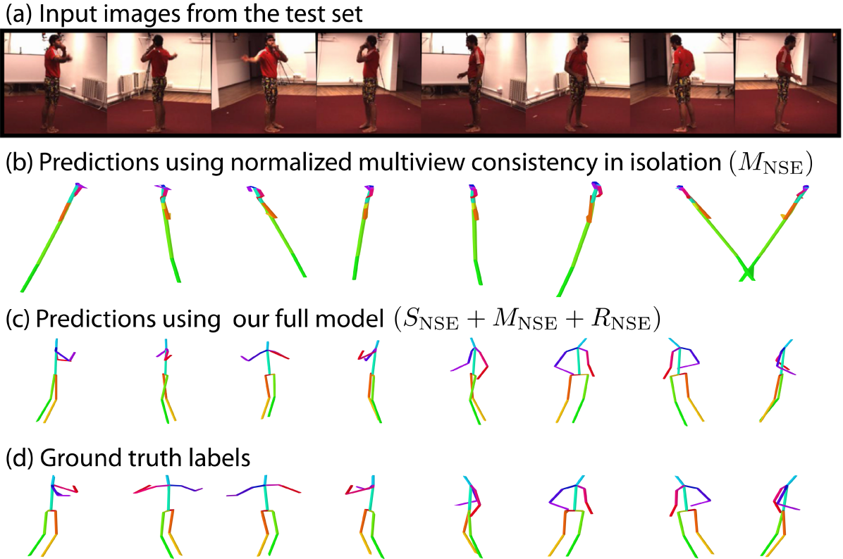
As illustrated by Fig. 3, only using the multi-view consistency loss would yield trivial solutions where all predicted poses would be random but identical. To prevent this, we propose to also use a small amount of supervised data. To this end, we define a loss that penalizes deviations between the predicted and ground-truth poses. We write it as

$$S_{C}(\theta,\mathcal{L})=\frac{1}{N_{s}}\sum_{i=1}^{N_{s}}C(f_{\theta}(\mathbf{I}_{i}),\mathbf{p}_{i})\;,$$ (6)

where $C$ is one of the distances introduced before, that is, it can be either the squared error of Eq. 3 or the scale-invariant version of Eq. 4.

Regularization Loss.

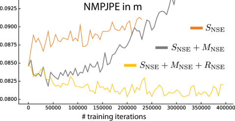
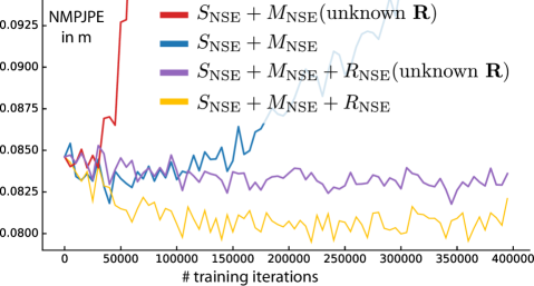
As shown in Fig. 7, using both $M(\cdot)$ and $S(\cdot)$ during training improves validation accuracy in the early training stages, thus showing the benefits of our multi-view weak supervision. However, after several epochs, the resulting model overfits, as indicated by the increasing error in Fig. 7. On closer examination, it appeared that the network learns to distinguish the labeled examples from the unlabeled ones and to, again, predict consistent but wrong poses for the latter, as depicted by Fig. 3 (b).

To prevent this, we introduce an additional regularization term $R_{C}(\theta,\mathcal{U})$, that penalizes predictions that drift too far away from the initial ones during training. To obtain these initial predictions, we use our scarce annotated data to begin training a network using only the loss $S$ and stop early to avoid overfitting, which corresponds to the 0 on the $x$-axis of Fig. 7. Let $\gamma$ be the parameters of this network. Assuming that the labeled poses are representative, the predictions $f_{\gamma}(\mathbf{I}_{t}^{c})$ for the unlabeled images will look realistic. We therefore write our regularizer as

$$R_{C}(\theta,\mathcal{U})=\frac{1}{N_{u}}\sum_{t=1}^{N_{u}}\frac{1}{n_{t}}\sum_{c=1}^{n_{t}}C(f_{\theta}(\mathbf{I}_{t}^{c}),f_{\gamma}(\mathbf{I}_{t}^{c}))\;.$$ (7)

In other words, we penalize 3D poses that drift too far away from these initial estimates. In principle, we could progressively update $\gamma$ during training. However, in practice, we did not observe any improvement and we keep it fixed in all experiments reported in this paper.

Our complete approach is summarized in Algorithm 1.

Data: Labeled training set $\mathcal{L}$ and unlabeled set $\mathcal{U}$

Result: Optimized neural network parameters $\theta$

Pre-training of $f_{\theta}$ on $\mathcal{L}$ through $S_{\text{NSE}}$

$\gamma\leftarrow\theta$

for # of gradient iterations do

      Select a random subset of 8 examples from $\mathcal{L}$

      Select 8 examples from $\mathcal{U}$ such that the first four ($n_{t}=4$) as well as the last four are taken at the same time $t$

      if $\mathbf{R}$ not available then

          Estimate rotations $\mathbf{R}_{t}^{c}$ for each quadruple

           Infer consensus sets $\Omega_{t}$

           Compute reference poses $\bar{\mathbf{p}}_{t}$

           Optimize $L_{f}(\theta)$ with respect to $\theta$ using Adam

Algorithm 1 Summary of our weakly supervised training method using the default parameters

Implementation Details.

We rely on the ResNet-50 architecture [7] up to level 5. In order to regress the pose vector output from convolutional features, we replace level 5 with two convolutional layers and a fully-connected layer. The first convolutional layer we added has a $3\times 3$ kernel size and 512 output channels. The second one has a $5\times 5$ kernel size and 128 output channels. The first three levels are initialized through transfer learning by pre-training on a 2D pose estimation task, as proposed by [16], and then kept constant. For the weak supervision experiments, the network is pre-trained on $\mathcal{L}$.

During training, we use mini-batches of size 16. Each one contains 8 labeled and 8 unlabeled samples. A consensus set size $|\Omega|$ of two was most effective in our examples. If more than four camera views are available, a random subset of cardinality four is chosen. Since the full objective function $L_{f}$ of Eq. 1 is the sum of three terms, their respective influence has to be adjusted. We have found empirically that weighting the supervised loss $S$ of Eq. 6 and regularizer $R$ of Eq. 7 by 100 and the unsupervised loss $M$ of Eq. 2 by 1 worked well for all experiments. We used the Adam optimizer with a constant learning rate of $0.001$. All examples in our training database are of resolution $256\times 256$, augmented by random rotations of $\pm 20^{\circ}$ and scaled by a factor between 0.85 and 1.15. Furthermore, we correct for the perspective effect as described in [16], which requires the camera intrinsics.

4 Results

In the following, we quantify the improvement of our weak-supervision approach and evaluate its applicability in diverse situations. We will provide videos and further qualitative results in the supplementary material.

Datasets.

We first test our approach on the well-known Human3.6M (H36M) [9] dataset to compare it to other state-of-the-art methods and on the more recent MPII-INF-3DHP (3DHP) set [16] to demonstrate how it generalizes to different viewpoints and outdoor scenes. In both cases, the images were recorded using a calibrated multi-camera setup, which makes these dataset easily exploitable for us.

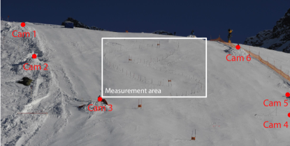
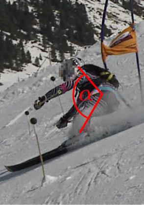
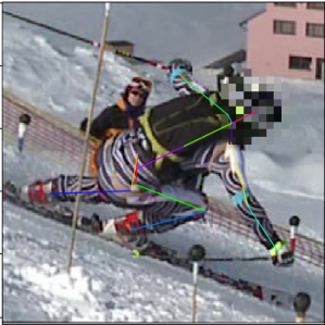
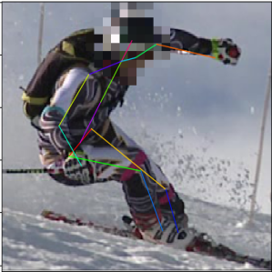
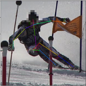
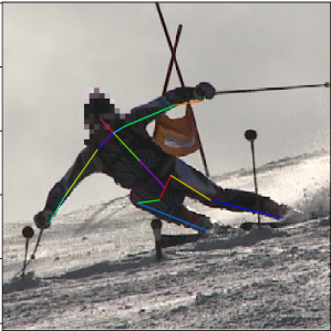
To highlight the effectiveness of our approach when using moving cameras to capture specialized motions that cannot be performed indoors, we also introduce a multi-view ski dataset that features competitive racers going down alpine slalom courses. The setup is shown in Fig. 4. Details on the capture and annotation process are explained in the supplemental document. Re-projection of the 3D annotation shows a very accurate overlap with the images, see Fig. 5. We make it available to facilitate future work towards reliable monocular pose reconstruction with weak supervision (cvlab.epfl.ch/Ski-PosePTZ-Dataset).

Figure 4: The alpine ski measurement setup. (Left) Six pan-tilt-zoom cameras are placed in a rough circle around the race course. (Right) Metrics such as hip flexion are commonly used for performance analysis.

Figure 5: Alpine ski dataset. The dataset provides six camera views as well as corresponding 3D pose. Four example views are shown. The 3D pose matches accurately when reprojected onto the input views, here shown by the stick-figure overlay.

Metrics.

Supervised training on all subjects of H36M
Training Sub.	Method	MPJPE in mm	NMPJPE in mm	PMPJPE in mm
Subjects S1+S5+S6+S7+S8	Pavlakos et al. [19]	118.4	not available	not available
	Rogez et al. [23]	87.7	not available	71.6
	Pavlakos et al. [18]	71.9	not available	51.9
	Zhou et al. [31]	64.9	not available	not available
	Mehta et al. [16]	74.1	68.6	54.6
	Tekin et al. [26]	69.7	not available	50.1
	Popa et al. [20]⋆	63.4	not available	not available
	Martinez et al. [15]	62.9	not available	47.7
	$S_{\text{SE}}$	66.8	63.3	51.6
	$S_{\text{NSE}}$	not applicable	64.2	53.0
Weakly-supervised training with varying training sets
Training Sub.	Method	MPJPE in mm	NMPJPE in mm	PMPJPE in mm
S1 only, known $\mathbf{R}$	$S_{\text{NSE}}$	not applicable	83.4	68.4
	$S_{\text{NSE}}+M_{\text{NSE}}+R_{\text{NSE}}$	not applicable	78.2	64.6
S1, unknown $\mathbf{R}$	$S_{\text{NSE}}+M_{\text{NSE}}+R_{\text{NSE}}$	not applicable	80.1	65.1
S1+S5, known $\mathbf{R}$	$S_{\text{NSE}}$	not applicable	76.1	61.8
	$S_{\text{NSE}}+M_{\text{NSE}}+R_{\text{NSE}}$	not applicable	70.8	58.5

Table 1: H36M results. (Top portion) In the fully supervised case, our comparatively simple network architecture is competitive when used in conjunction with the NSE distance function ($S_{\text{NSE}}$), but its performance is worse when used in conjunction with SE ($S_{\text{SE}}$). Note that the method of [20] (^⋆) uses silhouette information for training, which none of the other methods do. (Middle portion) Using a single subject to provide the supervised training set and enforcing the consistency constraints on the others ($S_{\text{NSE}}+M_{\text{NSE}}+R_{\text{NSE}}$) or not ($S_{\text{NSE}}$). (Bottom portion) Using two subjects to provide the supervised training set. In both cases, imposing the consistency constraints boosts the accuracy.

Weakly-supervised training with varying loss functions
Training Sub.	Method	MPJPE in mm	NMPJPE in mm
S1 only, known $\mathbf{R}$	$S_{\text{SE}}$	99.6	91.5
	$S_{\text{SE}}+M_{\text{SE}}+R_{\text{SE}}$	98.5	88.8
	$S_{\text{NSE}}$	not applicable	83.4
	$S_{\text{NSE}}+M_{\text{NSE}}+R_{\text{NSE}}$	not applicable	78.2
S1+S5, known $\mathbf{R}$	$S_{\text{SE}}$	90.3	77.5
	$S_{\text{SE}}+M_{\text{SE}}+R_{\text{SE}}$	89.0	74.7
	$S_{\text{NSE}}$	not applicable	76.1
	$S_{\text{NSE}}+M_{\text{NSE}}+R_{\text{NSE}}$	not applicable	70.8

Table 2: Different pose distances on H36M. Our multi-view constraint improves reconstructions, both with the commonly used SE distance ($S_{\text{SE}}+M_{\text{SE}}+R_{\text{SE}}$) and the normalized NSE version ($S_{\text{NSE}}+M_{\text{NSE}}+R_{\text{NSE}}$). However, reconstruction accuracy is higher and improvements are larger for the proposed normalized loss (compare second and fourth rows). This improvement is consistent across varied training sets (top vs. bottom portion).

We evaluate pose accuracy in terms of the mean per joint position error (MPJPE) and the percentage of correct keypoints (PCK), that is, the percentage of joints whose estimated position is within 15cm of the correct one. To make both measures independent from the subjects’ height, we systematically apply a single scale factor to the prediction so as to minimize the squared distance SE between label and prediction. We refer to the resulting normalized metrics as NMPJPE and NPCK. Since orientation is left unchanged, this is a less constraining transformation than the more commonly used Procrustes alignment, to which we refer as PMPJPE. For skiing, we also compute four specialized metrics commonly used in this scenario [3, 4]. The first two are the COM-hip joint distance and the COM-ankle distance being representative of relative COM position. The COM is computed from 3D pose according to the average body weight distribution [2]. The other two are the hip-flexion and knee-flexion angles. These metrics have been extensively used in sking related research before and are depicted by Fig. 4 (right).

Baseline.

In the top portion of Table 1, we report the MPJPE and NMPJPE values of fully-supervised methods on H36M using the same protocol as in [13, 31, 16, 26, 18, 19]: Five subjects (S1, S5, S6, S7, S8) are used for training and the remaining two (S9, S11) for testing. The 3D position of the 16 major human joints is predicted relative to the pelvis. The training and test sets are subsampled at 10fps, to reduce redundancy and validation time.

It shows that our modified ResNet-50 architecture, introduced in Section 3, yields results that are representative of the state-of-the-art methods, despite being considerably simpler—and also faster to train and experiment with. For example, the approach of [16] uses a residual network with twice as many layers as ours, along with a complex learning rate scheduling. The popular stacked-hourglass network used by some of the most recent methods [15, 31, 26] is even more complex, which results in long training and testing times of 32 ms per batch . The volumetric network of Pavlakos et al. [18] even takes 67 ms. Popa et al. [20] use a complex iterative multitask architecture and incorporate semantic segmentation, that is, labels that are not used by any of the other methods. This justifies choosing our modified ResNet-50 architecture, which has a runtime of only 11 ms .

For training the baseline, we test the NSE and SE loss using the dataset mean and standard deviation normalization as proposed by [25]. The NSE loss performs better than SE when the labeled training set is small and in combination with the multi-view constraint, see Table 2. We will refer to it as $S_{\text{NSE}}$ in the remainder of this section. Since our approach does not depend on the architecture of the base classifier, the slightly higher accuracies obtained by more complex ones would translate to our weakly-supervised results if we were to use them as our model.

4.1 Multi-View Supervision on Human3.6M

To test our multi-view weak supervision scheme, we split the standard training set into a supervised set $\mathcal{L}$ and an unsupervised one $\mathcal{U}$. In $\mathcal{L}$, we use the images and associated ground-truth poses, while in $\mathcal{U}$, we only use the camera orientation and bounding box crop information. In the bottom portion of Table 1, we report our results for two different splits: Either two subjects, S1 and S5, in $\mathcal{L}$ and the other three in $\mathcal{U}$, or only S1 in $\mathcal{L}$ and the other four in $\mathcal{U}$. The numbers we report are averages for all actions and we supply a detailed breakdown in the supplementary material. In both cases, the performance of $S_{\text{NSE}}$ trained only on $\mathcal{L}$ is lower than when using the full training set. Importantly, our approach ($S_{\text{NSE}}+M_{\text{NSE}}+R_{\text{NSE}}$) allows us to recover 5 mm in NMPJPE. That is, 28% and 42% of the difference to the full set is recovered, thus showing the benefits of our weak supervision. We show qualitative results in Fig. 6. In all these experiments, we used the known camera rotations. We will discuss what happens when we try to also recover the rotations below.

Figure 6: $S_{\text{NSE}}+M_{\text{NSE}}+R_{\text{NSE}}$ (yellow) and $S_{\text{NSE}}$ (orange) results overlaid on the ground truth label (black). Out of 2800 test images, the NMPJE is improved by more than 10 mm in 813 of them and degraded in only 259. Crouching and extreme stretching motions are improved most often.

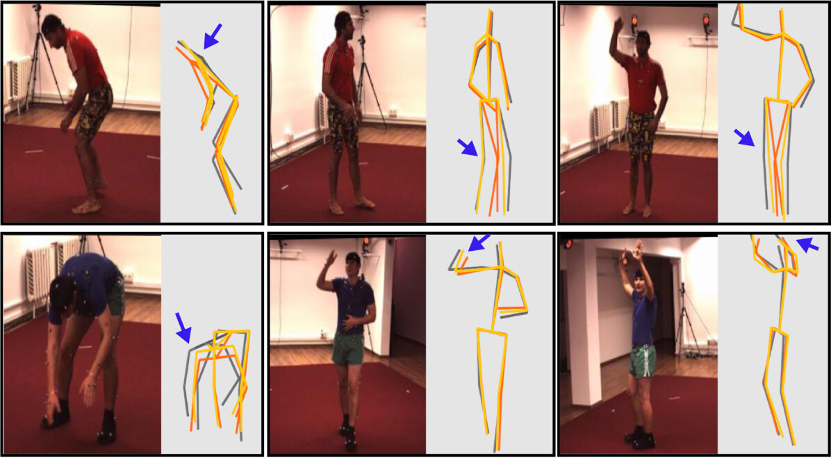
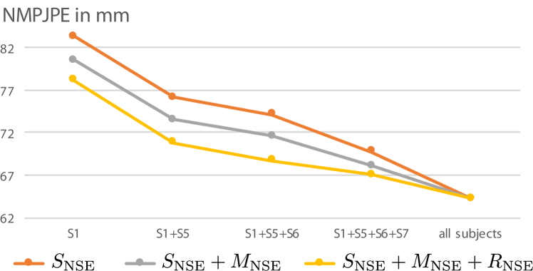
Fig. 8 summarizes these results. We plot the NMPJPE values as a function of the number of people in $\mathcal{L}$. As expected, the relative improvement brought about by our weak supervision is larger when we have fewer people in $\mathcal{L}$, and the order of the methods remains consistent throughout, with $S_{\text{NSE}}+M_{\text{NSE}}+R_{\text{NSE}}$ being best, followed by $S_{\text{NSE}}+M_{\text{NSE}}$ and $S_{\text{NSE}}$. The behavior is exactly the same when using NPCK instead of NMPJPE as error metric.

To demonstrate the importance of the regularization term of Eq. 7, we also trained our network using a loss function that is the sum of the multi-view loss of Eq. 2 and the supervised loss of Eq. 6, but without regularization. We refer to this as $S_{\text{NSE}}+M_{\text{NSE}}$, which we found much more difficult to train. As shown in Fig. 7, performing too many training iterations decreases accuracy, and we therefore had to resort to early stopping. Our complete model, with the additional regularization term, does not suffer from this issue.

Network initialization

Initializing the weights with ImageNet instead of pre-training on 2D human pose yields an error of 95.4 mm NMPJPE for our fully-supervised baseline. Using only S1 and S5 for supervision yields 159.0 mm. Using the unsupervised subjects S6-S8 improves by 16.1 mm, or 25.3 % of the gap. This is a larger absolute but slightly smaller relative improvement compared to the results obtained by pre-training on the MPII 2D pose dataset. For S1 our method improves from $161.4$ to $153.3$ and for $S1+S5+S6$ from $122.9$ to $114.5$. This shows that our multi-view approach can be applied as is, even in the absence of 2D annotations.

Figure 7: Validation error on H36M. Mean NMPJPE evaluated at equidistant points during training. With the normalized NSE loss the network performance improves initially, but needs early stopping since it diverges after 30k iterations. In combination with the regularizer $R_{\text{NSE}}$ the lowest error is attained.

Figure 8: Baselines and our full model evaluated on the Human3.6M dataset with varying number of subjects in the labeled set $\mathcal{L}$. Both, $S_{\text{SE}}$ and $S_{\text{NSE}}+M_{\text{NSE}}+R_{\text{NSE}}$ improve consistently.

Figure 9: Generalization to new camera views. (left) We overlay $S_{\text{NSE}}+M_{\text{NSE}}+R_{\text{NSE}}$ predictions in yellow, $S_{\text{NSE}}$ predictions in orange and GT in gray in top-down views that are not part of the training set. (right) Only labeled examples acquired by chest-height camera, like the rightmost image, were used for training.

4.2 Viewpoint Changes — MPII-3DHP

While the prediction accuracy of state-of-the-art methods on Human3.6M saturates at about 60mm, the recent MPII-3DHP dataset targets more challenging motions, such as gymnastics. Ground-truth joint positions were obtained via marker-less motion capture from 12 synchronized cameras, which allows the actors to wear more diverse clothing. We rely on the standard protocol: The five chest-hight cameras and the provided 17 joint universal skeletons are used for training and testing. Note that here we compare the methods in terms of the PCK and NPCK metrics, which are more widely used on this dataset and for which a higher value is better. Table 3 shows that our baseline $S_{\text{NSE}}$ is on par with existing methods when trained in a fully supervised manner either on H36M or 3DHP and tested on 3DHP. In the weakly-supervised case, with a single labeled subject, $S_{\text{NSE}}+M_{\text{NSE}}+R_{\text{NSE}}$ improves NPCK, as it did in the H36M experiments.

An interesting aspect of 3DHP is the availability of top-down and bottom-up views, which are missing from other pose datasets. This allows us to test the robustness of our approach to new camera views, as shown in Fig. 9. To this end, we train $S_{\text{NSE}}+M_{\text{NSE}}+R_{\text{NSE}}$with the standard views of S1 as strong supervision and with unlabeled examples from all the views—both standard and not—for S2 to S7. As shown in the bottom portion of Table 3, this greatly improves the predictions for the novel views of S8 compared to using the supervised data only.

Full H36M training, MPII-3DHP test set
Training	Method	NMPJPE in mm	PCK	NPCK
H36M	Mehta et al. [16]	not available	64.7	not available
	Zhou et al. [31]	not available	not available	69.2
	$S_{\text{NSE}}$	141.1	not applicable	66.9
Training and test on MPII-3DHP
Training	Method	NMPJPE in mm	PCK	NPCK
S1,S2,…,S8	Mehta et al. [16]	not available	$\mathbf{72.5}$	not available
	$S_{\text{NSE}}$	101.5	not applicable	$\mathbf{78.8}$
Supervised training on MPII-3DHP S1, weakly-supervised on S2 to S8
Training	Method	NMPJPE in mm	PCK	NPCK
S1, known $\mathbf{R}$	$S_{\text{NSE}}$	124.9	not applicable	71.6
	$S_{\text{NSE}}+M_{\text{NSE}}+R_{\text{NSE}}$	119.8	not applicable	73.1
S1, unknown $\mathbf{R}$	$S_{\text{NSE}}+M_{\text{NSE}}+R_{\text{NSE}}$	121.8	not applicable	72.7
Generalization to new viewpoints through weak supervision
(labeled S1, views [0, 2, 4, 7, 8]; unlabeled S2 to S7, views 0-9; test on S8, views [1,3,5,6,9])
Training	Method	NMPJPE in mm	PCK	NPCK
S1, known $\mathbf{R}$	$S_{\text{NSE}}$	125.4	not applicable	70.9
	$S_{\text{NSE}}+M_{\text{NSE}}+R_{\text{NSE}}$	108.7	not applicable	77.5

Table 3: Comparison to the state-of-the-art on MPII-3DHP. (Top 2 tables) In the fully-supervised case, when training either on H36M or on MPII-3DHP, our baselines $S_{\text{SE}}$ and $S_{\text{NSE}}$ yield NPCK (the higher the better) comparable to the state of the art, with a superior performance when exploiting our NSE metric. (Third table) In the weakly-supervised scenario, with a single labeled subject, $S_{\text{NSE}}+M_{\text{NSE}}+R_{\text{NSE}}$ provides a boost in accuracy over our baselines. (Fourth table) Our approach can also be used to improve accuracy on new viewpoints without having to rely on any labeled images from these viewpoints.

4.3 Outdoor Capture— Competitive Ski Dataset

In competitive skiing, the speeds are such that a static camera setup would cover a capture volume too small to acquire more than fractions of a turn. Therefore, most biomechanical studies rely on pan-tilt-zoom (PTZ) cameras to follow the racers over multiple turns, and their pose is estimated by manually annotating the images. The technique we propose here has the potential to eliminate the need for most of these annotations.

For our experiments, we have access to a training database that was used in an earlier methodological study [4]. Six pan-tilt-zoom cameras were used to capture six subjects during two runs each down a giant slalom course. See Fig. 4 for an overview. After manual annotation, followed by processing and filtering inaccurate poses, 10k temporal frames remained, which were split into 8481 for training (Subjects 1–5) and 1760 for testing (Subject 6).

The intrinsic and extrinsic camera parameters were estimated using geodetically measured reference points. In other words, the rotation $\mathbf{R}_{t}^{c}$ of camera $c$ with respect to the reference frame is precisely known for all cameras at all times. To test the ability of our approach to operate without this knowledge, we report results both when using these known rotations and when estimating them by solving the minimization problem of Eq. 5.

Figure 10: Bar plot of improvements of $S_{\text{NSE}}+M_{\text{NSE}}+R_{\text{NSE}}$ in comparison to the baseline $S_{\text{NSE}}$ on the task of ski-motion reconstruction for varying amount of labeled training data. Ski specific measurements, such as the knee flexion angle in degree, are measured alongside the NMPJPE.

Figure 11: Skiing reconstruction. Training with additional unsupervised data improves reconstruction in difficult cases that are not covered by $\mathcal{L}$, such as partial occlusion by snow and gate crossings, and extreme poses. We overlay $S_{\text{NSE}}+M_{\text{NSE}}+R_{\text{NSE}}$ predictions in yellow, $S_{\text{NSE}}$ predictions in orange and GT in gray.

Known rotations

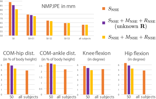
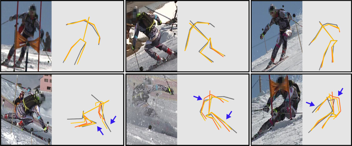
In Fig. 10, as before, we report our results as a function of the number of skiers used to form the supervised set $\mathcal{L}$, with the videos of the other ones being used to enforce the multi-view consistency constraints. We express our results in terms of NMPJPE, COM, hip-flexion, and knee-flexion angles. Altogether, $S_{\text{NSE}}+M_{\text{NSE}}+R_{\text{NSE}}$ systematically improves over $S_{\text{NSE}}$, with the improvement monotonically decreasing the more labeled data we use. In particular occlusions and extreme poses are improved, as depicted by Fig. 11.

Estimated rotations

The results shown above were computed assuming the rotations to be known, which was the case because the images were acquired using a very elaborate setup. To test the viability of our approach in a less constrained setup, such as one where the images are acquired using hand-held cameras, we repeated the above experiments without assuming the rotations to be known. The results are shown in Fig. 10 as purple bars. The improvement brought about by the weak supervision drops with respect to what it was when the rotations were given—for example from 7.4 to 3.4 mm in NMPJPE terms when using the motions of a single skier to form $\mathcal{L}$—but remains consistent. A similar improvement of 3-5 mm in NMPJPE is maintained on H36M and 3DHP, see the row below the dashed line in Tables 1 and 3.

Convergence.

In Fig. 12, we plot the training errors for the different versions of our approach, including $S_{\text{NSE}}+M_{\text{NSE}}$, the variant in which we minimize the multi-view consistency constraint but not the regularization term, for both known and estimated rotations. When regularizing, the loss remains well-behaved and attains a lower minimum in both cases, whereas it diverges when the regularizer is omitted, which confirms its importance.

Figure 12: Training error on H36M, with and without estimating the camera rotation $\mathbf{R}$ alongside the human pose $\mathbf{p}$. Training only converges with the proposed regularization term.

5 Conclusion

We have shown that a small annotated dataset of images and corresponding 3D poses could be effectively supplemented by a set of images acquired by multiple synchronized cameras using minimal amounts of supervision, even if their relative positions are not exactly known. At the heart of our approach are a multi-view consistency loss that encourages the regressor to predict consistent 3D poses in all views and a regularization loss that prevents the classifier from behaving differently on the annotated images and on the others. A key limitation of our current approach is that we work on individual images even though we are using video data. A clear next step will be to enforce temporal consistency both on the camera motions and the predictions at training time to increase performance. Our existing multi-view framework should make this relatively straightforward since multiple images acquired over time are not fundamentally different from multiple images acquired at the same time, except for the fact that the pose cannot be expected to be exactly the same.

References

- [1] W. Chen, H. Wang, Y. Li, H. Su, Z. Wang, C. Tu, D. Lischinski, D. Cohen-or, and B. Chen. Synthesizing Training Images for Boosting Human 3D Pose Estimation. In 3DV, 2016.
- [2] C. Clauser, J. McConville, and J. Young. Weight, Volume, and Center of Mass Segments of the Human Body. Journal of Occupational and Environmental Medicine, 13(5):270, 1971.
- [3] B. Fasel, J. Spörri, J. Chardonnens, J. Kröll, E. Müller, and K. Aminian. Joint inertial sensor orientation drift reduction for highly dynamic movements. IEEE journal of biomedical and health informatics, 22(1):77–86, 2018.
- [4] B. Fasel, J. Spörri, M. Gilgien, G. Boffi, J. Chardonnens, E. Müller, and K. Aminian. Three-dimensional body and centre of mass kinematics in alpine ski racing using differential gnss and inertial sensors. Remote Sensing, 8(8):671, 2016.
- [5] M. Fischler and R. Bolles. Random Sample Consensus: A Paradigm for Model Fitting with Applications to Image Analysis and Automated Cartography. Communications ACM, 24(6):381–395, 1981.
- [6] R. Garg, G. Carneiro, and I. Reid. Unsupervised CNN for Single View Depth Estimation: Geometry to the Rescue. In European Conference on Computer Vision, pages 740–756, 2016.
- [7] K. He, X. Zhang, S. Ren, and J. Sun. Deep Residual Learning for Image Recognition. In Conference on Computer Vision and Pattern Recognition, pages 770–778, 2016.
- [8] B. Horn. Closed-Form Solution of Absolute Orientation Using Unit Quaternions. Journal of the Optical Society of America, 4(4):629–642, April 1987.
- [9] C. Ionescu, J. Carreira, and C. Sminchisescu. Iterated Second-Order Label Sensitive Pooling for 3D Human Pose Estimation. In Conference on Computer Vision and Pattern Recognition, 2014.
- [10] C. Ionescu, O. Vantzos, and C. Sminchisescu. Matrix backpropagation for Deep Networks with Structured Layers. 2015.
- [11] H. Joo, H. Liu, L. Tan, L. Gui, B. Nabbe, I. Matthews, T. Kanade, S. Nobuhara, and Y. Sheikh. Panoptic Studio: A Massively Multiview System for Social Motion Capture. In International Conference on Computer Vision, 2015.
- [12] C. Lassner, J. Romero, M. Kiefel, F. Bogo, M. Black, and P. Gehler. Unite the People: Closing the Loop Between 3D and 2D Human Representations. In Conference on Computer Vision and Pattern Recognition, 2017.
- [13] S. Li and A. Chan. 3D Human Pose Estimation from Monocular Images with Deep Convolutional Neural Network. In Asian Conference on Computer Vision, 2014.
- [14] M. Loper, N. Mahmood, J. Romero, G. Pons-Moll, and M. Black. SMPL: A Skinned Multi-Person Linear Model. ACM SIGGRAPH Asia, 34(6), 2015.
- [15] J. Martinez, R. Hossain, J. Romero, and J. Little. A Simple Yet Effective Baseline for 3D Human Pose Estimation. In International Conference on Computer Vision, 2017.
- [16] D. Mehta, H. Rhodin, D. Casas, P. Fua, O. Sotnychenko, W. Xu, and C. Theobalt. Monocular 3D Human Pose Estimation in the Wild Using Improved CNN Supervision. In International Conference on 3D Vision, 2017.
- [17] D. Mehta, S. Sridhar, O. Sotnychenko, H. Rhodin, M. Shafiei, H. Seidel, W. Xu, D. Casas, and C. Theobalt. Vnect: Real-Time 3D Human Pose Estimation with a Single RGB Camera. In ACM SIGGRAPH, 2017.
- [18] G. Pavlakos, X. Zhou, K. Derpanis, G. Konstantinos, and K. Daniilidis. Coarse-To-Fine Volumetric Prediction for Single-Image 3D Human Pose. In Conference on Computer Vision and Pattern Recognition, 2017.
- [19] G. Pavlakos, X. Zhou, K. D. G. Konstantinos, and D. Kostas. Harvesting Multiple Views for Marker-Less 3D Human Pose Annotations. In Conference on Computer Vision and Pattern Recognition, 2017.
- [20] A.-I. Popa, M. Zanfir, and C. Sminchisescu. Deep Multitask Architecture for Integrated 2D and 3D Human Sensing. In Conference on Computer Vision and Pattern Recognition, 2017.
- [21] H. Rhodin, C. Richardt, D. Casas, E. Insafutdinov, M. Shafiei, H.-P. Seidel, S. B, and C. Theobalt. Egocap: Egocentric Marker-Less Motion Capture with Two Fisheye Cameras. ACM SIGGRAPH Asia, 35(6), 2016.
- [22] G. Rogez and C. Schmid. Mocap Guided Data Augmentation for 3D Pose Estimation in the Wild. In Advances in Neural Information Processing Systems, 2016.
- [23] G. Rogez, P. Weinzaepfel, and C. Schmid. Lcr-Net: Localization-Classification-Regression for Human Pose. In Conference on Computer Vision and Pattern Recognition, 2017.
- [24] T. Simon, H. Joo, I. Matthews, and Y. Sheikh. Hand keypoint detection in single images using multiview bootstrapping. In Conference on Computer Vision and Pattern Recognition, volume 2, 2017.
- [25] X. Sun, J. Shang, S. Liang, and Y. Wei. Compositional human pose regression. In International Conference on Computer Vision, volume 2, 2017.
- [26] B. Tekin, P. Márquez-neila, M. Salzmann, and P. Fua. Learning to Fuse 2D and 3D Image Cues for Monocular Body Pose Estimation. In International Conference on Computer Vision, 2017.
- [27] D. Tome, C. Russell, and L. Agapito. Lifting from the Deep: Convolutional 3D Pose Estimation from a Single Image. In arXiv preprint, arXiv:1701.00295, 2017.
- [28] S. Tulsiani, T. Zhou, A. Efros, and J. Malik. Multi-view supervision for single-view reconstruction via differentiable ray consistency. In Conference on Computer Vision and Pattern Recognition, volume 1, page 3, 2017.
- [29] G. Varol, J. Romero, X. Martin, N. Mahmood, M. Black, I. Laptev, and C. Schmid. Learning from synthetic humans. In Conference on Computer Vision and Pattern Recognition, 2017.
- [30] X. Yan, J. Yang, E. Yumer, Y. Guo, and H. Lee. Perspective Transformer Nets: Learning Single-View 3D Object Reconstruction Without 3D Supervision. In Advances in Neural Information Processing Systems, pages 1696–1704. 2016.
- [31] X. Zhou, Q. Huang, X. Sun, X. Xue, and Y. We. Weakly-Supervised Transfer for 3D Human Pose Estimation in the Wild. arXiv Preprint, 2017.