Hydrodynamics of Diffusion in Lipid Membrane Simulations

Abstract

By performing molecular dynamics simulations with up to 132 million coarse-grained particles in half-micron sized boxes, we show that hydrodynamics quantitatively explains the finite-size effects on diffusion of lipids, proteins, and carbon nanotubes in membranes. The resulting Oseen correction allows us to extract infinite-system diffusion coefficients and membrane surface viscosities from membrane simulations despite the logarithmic divergence of apparent diffusivities with increasing box width. The hydrodynamic theory of diffusion applies also to membranes with asymmetric leaflets and embedded proteins, and to a complex plasma-membrane mimetic.

Molecular dynamics (MD) simulations provide insight into the organization and dynamics of lipids and membrane proteins Pluhackova and Böckmann (2015); Ingólfsson et al. (2016); Hedger et al. (2016); Duncan et al. (2017). Receptor clustering, lipid second-messenger patterning, and lipid domain formation occur in systems with complex lipid composition Ingólfsson et al. (2014) on length scales $\geq$100 nm. Advances in computing, coarse-grained force fields Marrink et al. (2007); Cooke et al. (2005); Izvekov and Voth (2005), and simulation management Wassenaar et al. (2015); Stansfeld et al. (2015); Wu et al. (2014) open up this biologically important regime to simulations Ingólfsson et al. (2016); Koldsø et al. (2016); Lyman et al. (2018). However, simulations of dynamics in membranes face a serious challenge: the translational diffusion coefficients of membrane-embedded molecules are ill-defined. As anticipated from hydrodynamic theory Camley et al. (2015) and shown by MD simulations Vögele and Hummer (2016); Venable et al. (2017), the apparent diffusion coefficients diverge logarithmically with the size of the simulated membrane patch. One can think of a membrane particle and its periodic images above and below as forming an infinite quasi-cylindrical structure embedded in a layered medium that effectively imposes 2D flows. In this picture, the logarithmic divergence of the diffusion coefficient is a molecular-scale manifestation of Stokes’ paradox, i.e., the vanishing hydrodynamic friction of an infinite cylinder in an infinite medium with 2D flow. The divergence appears to preclude a meaningful comparison between simulation and experiment for membrane dynamic processes.

Here we show that hydrodynamic theory Camley et al. (2015); Vögele and Hummer (2016) can be used to overcome this challenge, as in neat fluids Yeh and Hummer (2004). First, we show that the logarithmic divergence can be broken by expanding the system also in the third dimension, normal to the membrane. This requires simulations with $\geq$10⁸ coarse-grained particles. Then we show that the Oseen correction, a hydrodynamic correction using the Oseen tensor for a point perturbation Vögele and Hummer (2016), quantitatively accounts for the observed behavior, from lipids to membrane proteins and over the entire range of box widths and heights. On this basis, we develop a procedure to correct the simulated diffusion coefficient. By exploiting the strong finite-size dependence, we not only extract the true infinite-system diffusion coefficients $D_{0}$ of lipids or embedded proteins, but also the difficult-to-obtain membrane surface viscosity $\eta_{m}$. We apply the formalism to simulations of the diffusion of proteins embedded in lipid membranes, and of a plasma-membrane model with a complex lipid composition.

For neat Dünweg and Kremer (1993); Yeh and Hummer (2004) and confined fluids Simonnin et al. (2017), hydrodynamic self-interactions under periodic boundary conditions (PBC) account for the system-size dependence of self-diffusion coefficients ${D}_{\mathrm{PBC}}$ in MD simulations,

$${D}_{\mathrm{PBC}}={D}_{0}+k_{\mathrm{B}}T\lim_{r\to 0}\mathrm{Tr}[\mathbf{T}^{\mathrm{PBC}}(\vec{r})-\mathbf{T}_{0}(\vec{r})]/n_{d}$$ (1)

In the Oseen correction, $\Delta D=D_{\mathrm{PBC}}-D_{0}$ is approximated as the difference between the Oseen tensors $\mathbf{T}^{\mathrm{PBC}}(\vec{r})$ for PBC and $\mathbf{T}_{0}(\vec{r})$ for the infinite system at the origin, $r\to 0$, with $\mathrm{Tr}$ the trace, $n_{d}$ the dimension ($n_{d}=2$ for membranes), $k_{\mathrm{B}}$ the Boltzmann constant, and $T$ the absolute temperature.

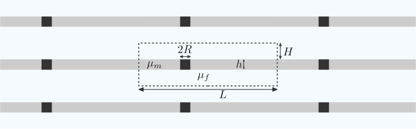
This formulation suggests hydrodynamic corrections also for membrane simulations Camley et al. (2015); Vögele and Hummer (2016). In the Saffman-Delbrück (SD) model Saffman and Delbrück (1975); Hughes et al. (1981); Petrov and Schwille (2008), the membrane is treated as a viscous fluid embedded in an infinite solvent system. Camley et al. Camley et al. (2015) extended the SD model to PBC by representing the Oseen tensor as a two-dimensional lattice sum, $T^{\mathrm{PBC}}_{ij}(\vec{r})=L_{x}^{-1}L_{y}^{-1}\sum_{\vec{k}\neq 0}\tau_{ij}(\vec{k})\,\exp(-i\vec{k}\cdot\vec{r})$, where $\tau_{ij}(\vec{k})=(\delta_{ij}-{k_{i}k_{j}}/{k^{2}})/(\eta_{m}k^{2}+2\eta_{f}k\tanh(kH))$. The ratio of membrane-surface and solvent viscosities $\eta_{m}$ and $\eta_{f}$, respectively, defines the SD length $L_{\mathrm{SD}}=\eta_{m}/2\eta_{f}$. The wave vectors are $\vec{k}=2\pi(n_{x}/L_{x},n_{y}/L_{y})$ with $n_{i}$ integers and $L_{i}$ the box widths ($i=x,y$), $k=|\vec{k}|$, and $\delta_{ij}$ the Kronecker delta. $2H=L_{z}-h$ is the height of the solvent layer separating the periodic images of the membrane, with $h$ the membrane thickness and $L_{z}$ the box height. The $\tanh$ term accounts for the influence of the surrounding solvent on the diffusion inside the membrane. An Oseen tensor for monotopic inclusions (spanning only one leaflet, such as typical lipids) was proposed as Camley et al. (2015): $\tau_{ij}(\vec{k})=(\delta_{ij}-{k_{i}k_{j}}/{k^{2}}){A(k)}/({A(k)^{2}-B(k)^{2}})$, with $A(k)=\eta_{m}k^{2}/2+\eta_{f}k/\tanh(2Hk)+b$, $B(k)=\eta_{f}k/\sinh(2Hk)+b$, and $b$ the interleaflet friction coefficient. We sped up convergence of the lattice sums in Eq. (1) by adding and subtracting integrals Vögele and Hummer (2016) that can be solved analytically for the transmembrane case and numerically for the monotopic case (see Supplemental Material SI ). All correction formulas are implemented in Python and available at https://github.com/bio-phys/memdiff along with an example application.

For the diffusion in membranes contained in flat square simulation boxes, $L=L_{x}=L_{y}\gg L_{z}$, one has Vögele and Hummer (2016)

$$D_{\mathrm{PBC}}\approx D_{0}+\frac{k_{\mathrm{B}}T}{4\pi\eta_{m}}\frac{\ln\left(L/(L_{\mathrm{SD}}+1.565H)\right)-1.713}{\left(1+H/L_{\mathrm{SD}}\right)}$$ (2)

Accordingly, $D_{\mathrm{PBC}}$ diverges asymptotically as $\ln L$ for large widths $L$ and fixed height $H$ (or $L_{z}$). This approximation is also valid for narrow boxes, $L<L_{\mathrm{SD}}$, if one sets $H=0$ instead of using the actual value Vögele and Hummer (2016). At a box width of $L_{c}\approx\left(L_{\mathrm{SD}}+1.565H\right)\,e^{1.713}$, in-plane and between-membrane self-interactions effectively cancel, and the box-size corrections vanishes, $D_{\mathrm{PBC}}\approx D_{0}$. In numerical tests, the flat-box approximation Eq. (2) is within 2 % of Eq. (1) for atomistic and coarse-grained systems (see Supplemental Material SI ). The hydrodynamic correction (but not $D_{0}$!) is insensitive to variations in the interleaflet friction coefficient $b$ for typical lipid models (see Supplemental Material SI ). The simpler transmembrane correction is thus expected to be an excellent approximation also for monotopic molecules such as individual lipids.

Figure 1: Diffusion coefficients of POPC lipids from MD simulations (symbols) as function of the height $H$ of the water layers above and below the membrane in simulation boxes of constant width $L=0.42\,\mu$m (top axis: number of particles in the system). The prediction according to Eq. (1) with the transmembrane Oseen tensor is shown as orange dashed line. $D_{0}$ and $\eta_{m}$ were fitted to POPC membrane simulations in flat boxes Vögele and Hummer (2016) and $\eta_{f}$ was determined independently from pressure fluctuations in bulk water simulations (SI, ). Horizontal lines indicate the true diffusion coefficient $D_{0}$ (green) and the limit $H\to\infty$ for fixed $L$ (red). Shading indicates the uncertainty range (1 s.d.).

Key open questions are: (1) does the Oseen correction apply beyond the flat-box limit with its logarithmically divergent $D_{\mathrm{PBC}}$; (2) how can one extract meaningful diffusion coefficients from membrane simulations; and (3) does a simple materials parameter, $\eta_{m}$, suffice to describe the dynamics in complex asymmetric membranes? To address the first challenge, we performed simulations with boxes large also normal to the membrane, $L_{z}\gg L_{\mathrm{SD}}$. To be consistent with Vögele and Hummer (2016), we simulated lipid membranes using the MARTINI coarse-graining scheme Marrink et al. (2007) and the GROMACS 4.5.6. software package Hess et al. (2008). The bilayer structures were built using insane.py Wassenaar et al. (2015). Water was added to reach the desired box heights. Because undulations of the lipid bilayer shorten the distance of lipid motions projected onto the $x$-$y$ plane, we suppressed long-wavelength undulations by a weak harmonic restraint acting on the $z$ coordinate of the center of mass of a quarter of the lipids Ingólfsson et al. (2014); Vögele and Hummer (2016). With these restraints, we assure a constant wavelength spectrum of undulations over all box sizes. Otherwise, long-wavelength undulations would only be suppressed in small boxes, with the longest wavelengths permitted under PBC being $L_{x}$ and $L_{y}$. Energy minimization was followed by equilibration and data production runs in an NPT Berendsen et al. (1984); Bussi et al. (2007) ensemble with semiisotropic pressure coupling at 1 bar and 300 K. Simulation details are listed in the Supplemental Material SI .

We obtained diffusion coefficients and viscosities by minimizing $\chi^{2}=\sum_{i=1}^{N}(D_{i}-D_{\mathrm{PBC}}^{(i)})^{2}/\sigma_{i}^{2}$ with respect to $D_{0}$ and $\eta_{m}$, treating $\eta_{f}$ either as an additional parameter in the minimization or fixing it at the bulk water viscosity, as determined from independent simulations. $i$ indexes the $N$ runs with different box sizes. $D_{i}$ is the uncorrected diffusion coefficient of run $i$ and $D_{\mathrm{PBC}}^{(i)}=D_{0}+\Delta D^{(i)}$ with $\Delta D^{(i)}$ the Oseen finite-size correction Eq. (1) evaluated numerically for fixed membrane thickness $h=4.5$ nm as described in Supplemental Material SI .

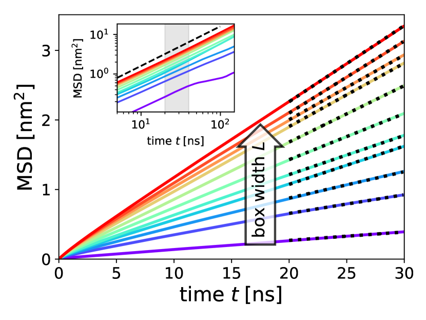
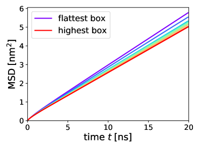
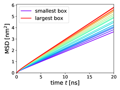
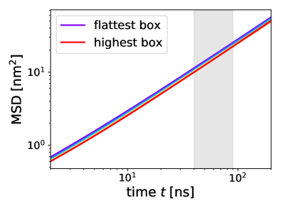
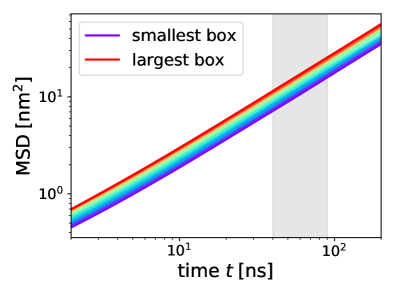
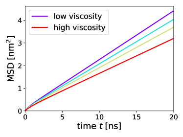
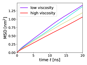
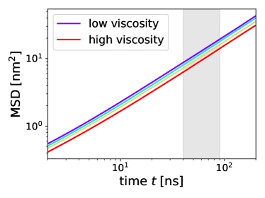
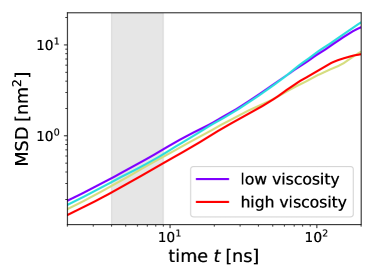
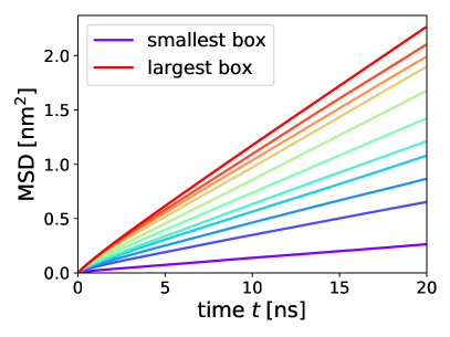
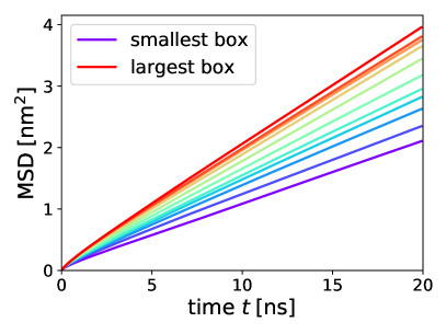
The $D_{i}$ were determined from the slopes of straight-line fits to the mean-squared displacement (MSD) in the membrane plane Vögele and Hummer (2016) over a time window from 40-90 ns for lipids, 4-9 ns for membrane-spanning carbon nanotubes (CNT; see Vögele and Hummer (2016); Vögele et al. (2018) for details on the CNT model), and 20-40 ns for integral membrane proteins, using shorter times for the latter two because their low abundance affects the sampling at longer times. We calculated the MSD with a Fourier-based algorithm Calandrini et al. (2011), after removing the center-of-mass motion of the membrane from lipid, protein, and CNT trajectories. Statistical errors $\sigma_{i}$ were estimated by block averaging using 20 blocks.

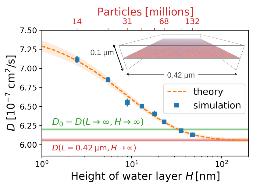
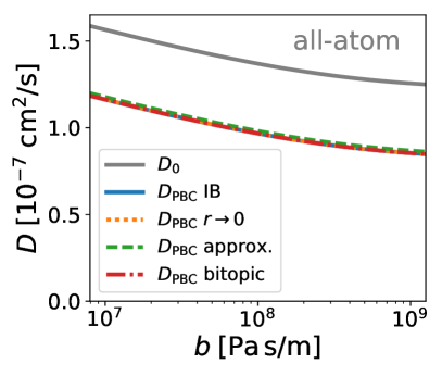
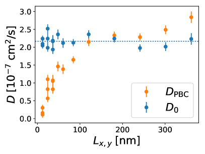
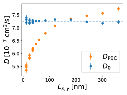
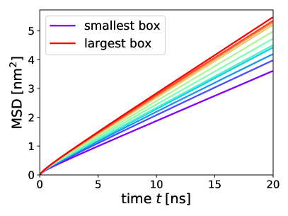
Figure 1 shows that Eq. (1) accounts quantitatively for the calculated diffusion coefficients for systems with up to 132 million particles in simulation boxes $L=0.42\,\mu$m wide and up to $L_{z}=0.1\,\mu$m tall. The simulation results match the hydrodynamic predictions using $\eta_{m}$ fitted only to flat-box simulations Vögele and Hummer (2016) and $\eta_{f}=10.2(4)$ determined independently from pressure fluctuations Hess (2002) of bulk MARTINI water. From a global fit of the transmembrane Oseen correction against all POPC simulations here and in Vögele and Hummer (2016), we obtained $D_{0}=6.20(2)\times 10^{-7}$ cm²/s, $\eta_{f}=9.6(2)\times 10^{-4}$ Pa s, and $\eta_{m}=3.97(6)\times 10^{-11}$ Pa s m, so that $L_{\mathrm{SD}}=20.7$ nm. The monotopic correction with $b=2.9\times 10^{6}$ Pa s/m den Otter and Shkulipa (2007); SI gives an indistinguishable fit with the same $D_{0}$, $\eta_{f}=10.17(20)\times 10^{-4}$ Pa s, and $\eta_{m}=4.05(6)\times 10^{-11}$ Pa s m. Thicker water layers weaken between-membrane hydrodynamic interactions and slow down lipid diffusion. For the tallest systems, $D_{\mathrm{PBC}}$ approaches a plateau. However, even with $10^{8}$ particles, the turnover is incomplete. The limit for $H\to\infty$ is below $D_{0}$; i.e., for tall boxes, hydrodynamics retards diffusion.

Figure 2: Dependence of diffusion coefficients $D_{\mathrm{PBC}}$ and $D_{0}$ of POPC lipids and CNTs Vögele and Hummer (2016) on water viscosity $\eta_{f}$ ($L=40$ nm, $L_{z}=9$ nm, 300 K). Lines show theory (Eq. (1) and $D_{0}^{\mathrm{SD}}$). Vertical line: $\eta_{f}$ for standard MARTINI water.

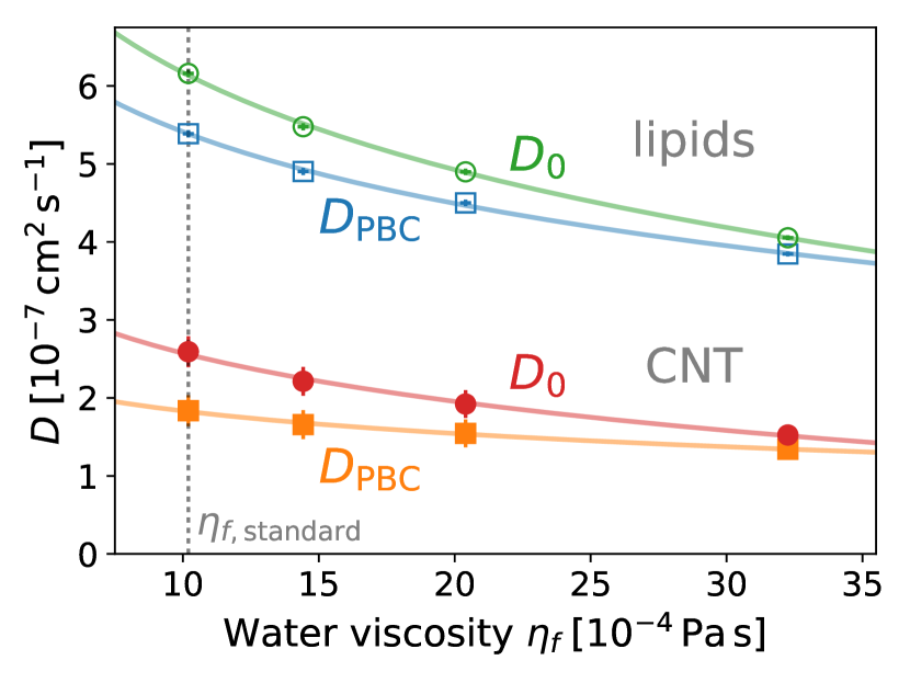
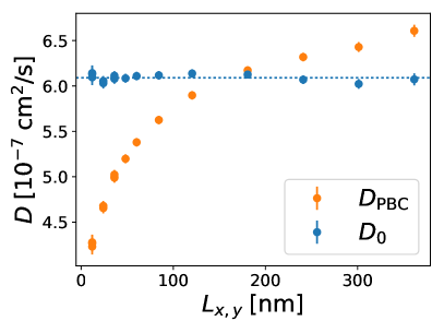
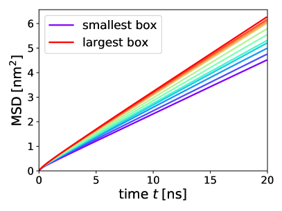
As an additional test of the hydrodynamic model, we examined the effect of water viscosity on diffusion in the membrane (Fig. 2). We reduced the SD length $L_{\mathrm{SD}}$ by increasing the mass $M$ of MARTINI water particles up to 10-fold, scaling the water viscosity as $M^{1/2}$ without altering the structure and thermodynamics of the system. For large $\eta_{f}$, $L_{\mathrm{SD}}$ becomes small and $D_{\mathrm{PBC}}$ approaches the infinite-box limit $D_{0}$. As shown in Fig. 2, the water viscosity dependence of the diffusion coefficients both of lipids in a neat membrane and of membrane-spanning CNTs quantitatively agrees with the predictions of Eq. (1), further validating the hydrodynamic model.

We determined hydrodynamic radii $R_{h}$ of diffusing molecules by setting their $D_{0}$ equal to the SD expression for the diffusion coefficient Saffman and Delbrück (1975), $D_{0}^{\mathrm{SD}}=k_{\mathrm{B}}T(4\pi\eta_{m})^{-1}(\ln(\eta_{m}/\eta_{f}R_{h})-\gamma)$ with $\gamma\approx 0.5772$ the Euler-Mascheroni constant. For the CNT, a fit to the data in Vögele and Hummer (2016) gave $D_{0}=2.76(12)\times 10^{-7}$ cm²/s. The resulting hydrodynamic radius of $R_{h}=0.83(14)$ nm agrees with the geometric value of 0.85 nm for this ideal cylinder obtained by summing the radii of the cylinder (0.615 nm) and a carbon bead (0.235 nm). Values of $D_{\mathrm{PBC}}\leq 1.9\times 10^{-7}$ cm²/s without hydrodynamic correction would have given unphysical radii $R_{h}\geq 2.3$ nm.

Figure 3: MSD of protein ANT1 in model mitochondrial membrane simulated in boxes of widths from $L=12$ nm (purple) to 360 nm (red) at constant box height $L_{z}=10.2$ nm ($H=2.85$ nm). Dotted black lines show fits of $\mathrm{MSD}(t)=a+4Dt$ over the time window used to extract the uncorrected diffusion coefficients $D$. The intercept $a$ accounts for local and fast molecular motions before proper diffusion sets in. In the double-logarithmic inset, the dashed line indicates a linear dependence on time. The fitting region is highlighted in gray.

Figure 4: Diffusion in complex membranes. Upper left: Model inner mitochondrial membrane ($L=360$ nm) with 900 ANT1 transmembrane proteins (yellow; see zoom-in). Lower left: $D_{\mathrm{PBC}}$ (symbols) and fits to hydrodynamic theory (protein: circles and solid lines; outer leaflet: stars and dotted lines; inner leaflet: squares and dashed lines), and infinite-system values (horizontal lines). Upper right: Plasma-membrane simulation ($L=286$ nm). Lower right: $D_{\mathrm{PBC}}$ for representative membrane components that remain in each leaflet (inner/outer) and for those that jump between both leaflets (“both”). Vertical gray lines indicate $L=L_{c}$, where $D_{\mathrm{PBC}}=D_{0}$. Corrections here were calculated using Eq. (2).

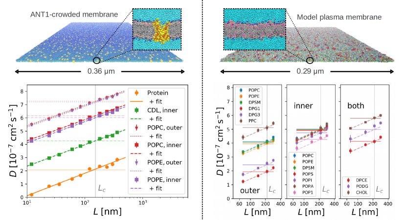
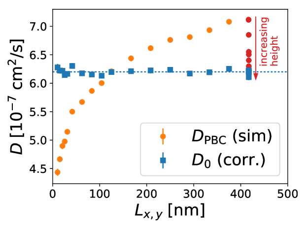
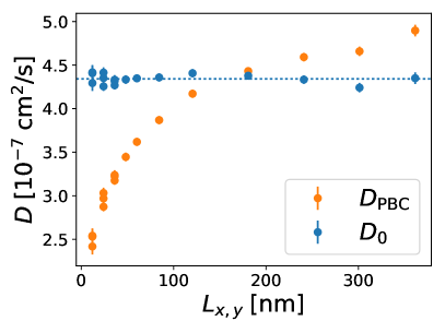
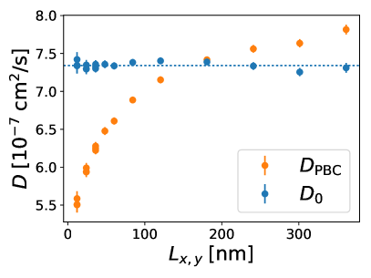
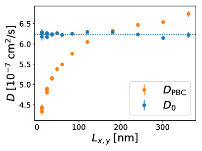
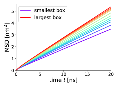
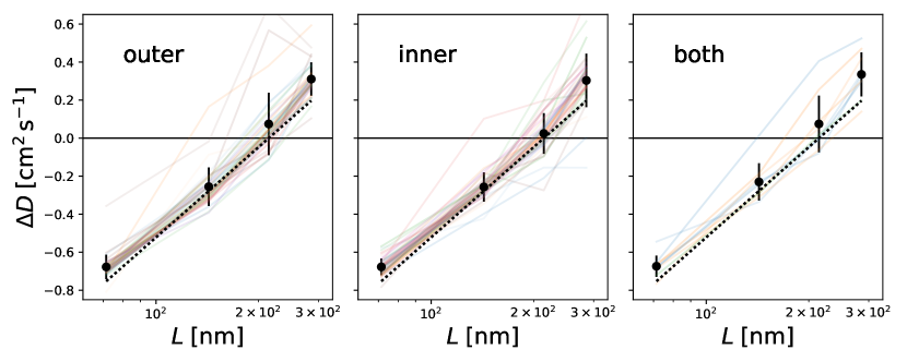
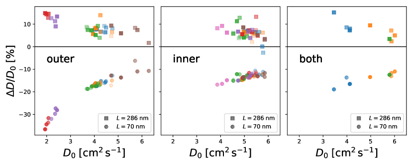
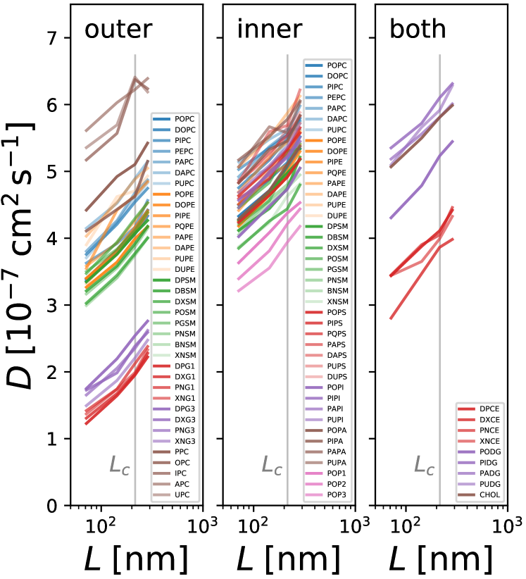
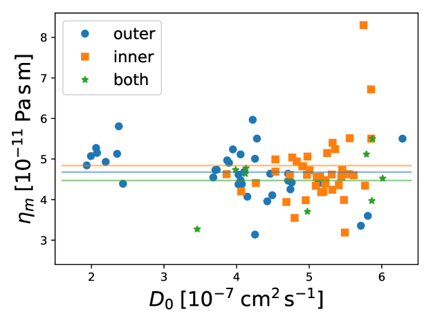
Hydrodynamic theory also accounts for the dramatic box-size dependence of membrane protein diffusion (Fig. 3). As a model inner mitochondrial membrane, we simulated a POPC/POPE membrane densely packed with the membrane-spanning protein adenine nucleotide translocase (ANT1) and with cardiolipin in the inner leaflet Hedger et al. (2016). Systems were built with MemProtMD Stansfeld et al. (2015) for a wide range of box widths $L$ (Fig. 4 upper left) at fixed heights $H$, such that proteins covered $\approx$11 % of the membrane area while not yet forming large clusters within the simulation time. In simulations using the parameters of Hedger et al. (2016), the proteins and different lipid components exhibit the same finite-size dependence (Fig. 4 lower left). Despite variations by about a factor 50 for the smallest systems, the apparent diffusivities $D_{\mathrm{PBC}}$ grow linearly as function of $\ln L$ with component-independent slopes, as predicted by the Oseen correction. Diffusion of POPC and POPE is slower in the inner leaflet by about 20 %, likely due to the presence of the large cardiolipin molecules. The ANT1 mitochondrial model membrane has an effective viscosity $\eta_{m}\approx 4.36\times 10^{-11}$ Pa s m, and ANT1 has a hydrodynamic radius of $R_{h}=2.1(4)$ nm, close to $R_{h}=2.3$ nm estimated from the convex hull in the $xy$ plane. By contrast, uncorrected diffusion coefficients would have given $R_{h}$ from 0.7 to 24.3 nm.

The Oseen correction also applies to membranes of even more complex composition. Figure 4 (right) shows that finite system sizes affect the diffusion in a plasma-membrane model Ingólfsson et al. (2014). We used the simulation parameters and the configuration provided at http://cgmartini.nl and built start configurations as squares of 1, 4, 9, and 16 copies of the original box. Even without clear phase separation Ingólfsson et al. (2014), heterogeneous structures emerged as small clusters of lipids. Moreover, molecules such as cholesterol flipped between the leaflets. Nevertheless, the slope of the apparent diffusion coefficients $D_{\mathrm{PBC}}$ with respect to $\ln L$ is independent of membrane component and leaflet localization, defining an effective membrane viscosity $\eta_{m}\approx 4.73\times 10^{-11}$ Pa s m according to Eq. (2) (Fig. 4 lower right). Even in asymmetric membranes of complex composition, a component-independent correction compensates for large finite-size effects.

We showed that finite-size effects in membrane simulations can be corrected by hydrodynamic theory. The Oseen corrections are independent of membrane component. Complex lipid composition and integral membrane proteins do not alter the effects in absence of protein clustering Duncan et al. (2017), strong protein crowding Javanainen et al. (2017), and phase segregation. With the Oseen correction Eq. (1) and its approximation Eq. (2), two simulations in flat boxes of different widths $L$ suffice to determine proper membrane diffusion coefficients $D_{0}$ and membrane viscosities $\eta_{m}$, using $\eta_{f}$ from independent bulk-solvent simulations. Thermostats are used in standard protocols for membrane MD simulations. Nevertheless, for weakly coupled rescaling thermostats Berendsen et al. (1984); Bussi et al. (2007), the diffusion of lipids, proteins, and nanotubes in membranes follows the predictions of hydrodynamic theory with respect to the dependence on system size and water viscosity. Based on the remarkable accuracy in capturing the dynamics of complex lipid membranes, we expect the hydrodynamic model to apply to transport phenomena also in other 2D layered materials.

I Acknowledgments

We thank Frank L. H. Brown, Richard W. Pastor, Lukas S. Stelzl, and Max Linke for helpful discussions. We acknowledge PRACE for access to Mare Nostrum at the Barcelona Supercomputing Centre. Further computations were performed on Hydra at the Max Planck Computing and Data Facility Garching. This work was supported by the Max Planck Society.

I Theoretical Details

Figure S1: Cut through a schematic simulation box (dashed lines) of a lipid membrane (gray) with surrounding periodic images according to the Saffman-Delbrück model. The membrane itself is treated as a fluid layer of height $h$ and viscosity $\eta_{m}$ immersed in a fluid (light blue) of viscosity $\eta_{f}$, with a cylindrical inclusion (black) of radius $R$.

I.1 Numerical Evaluation of the Correction Formulas for Transmembrane and Monotopic Inclusions

The numerical evaluation of the correction formula for transmembrane inclusions was described in Vögele and Hummer (2016). We subtract the long-wavelength part from the lattice sum and approximate it by an integral that can be solved analytically:

$$2\Delta T^{\mathrm{trans}} \equiv \frac{1}{L^{2}}\sum_{\vec{k}(\neq 0)}\frac{1}{\eta_{m}k^{2}+2\eta_{f}k\tanh(kH)}-\int\frac{d^{2}k}{(2\pi)^{2}}\frac{1}{\eta_{m}k^{2}+2\eta_{f}k}$$ (S1)

$$= \lim_{\sigma\to\infty}\Bigg{[}\frac{1}{L^{2}}\sum_{\vec{k}(\neq 0)}\Bigg{(}\frac{1}{\eta_{m}k^{2}+2\eta_{f}k\tanh(kH)}-\frac{1-e^{-k^{2}/2\sigma^{2}}}{\eta_{m}k^{2}+2\eta_{f}k}\Bigg{)}-\frac{e^{-u^{2}}\left[\pi\,\mathrm{erfi}(u)-E_{i}(u^{2})\right]}{4\pi\eta_{m}}\Bigg{]},$$ (S2)

where $\Delta T=\lim_{r\to 0}\mathrm{Tr}[\mathbf{T}_{\mathrm{PBC}}(\vec{r})-\mathbf{T}_{0}(\vec{r})]/2$, $u=\sqrt{2}\eta_{f}/\eta_{m}\sigma$, $\mathrm{erfi}(x)$ is the imaginary error function, and $E_{i}(x)$ the exponential integral.

In the monotopic case (an inclusion only within one leaflet or a lipid), we follow the same strategy, with the difference that the integral is solved numerically instead of analytically. Again, we first perform the subtraction of the long-wavelength part:

$$2\Delta T^{\mathrm{mono}} \equiv \frac{1}{L^{2}}\sum_{\vec{k}(\neq 0)}\frac{A(k)}{A(k)^{2}-B(k)^{2}}-\int\frac{\mathrm{d}^{2}k}{(2\pi)^{2}}\left[\frac{A(k)}{A(k)^{2}-B(k)^{2}}\right]_{H\rightarrow\infty}$$

$$= \frac{1}{L^{2}}\sum_{\vec{k}(\neq 0)}\left[\frac{A(k)}{A(k)^{2}-B(k)^{2}}-\frac{\eta_{\mathrm{mono}}k^{2}+\eta_{f}k+b}{(\eta_{\mathrm{mono}}k^{2}+\eta_{f}k+b)^{2}-b^{2}}\right]$$

$$+ \lim_{\sigma\to\infty}\Bigg{[}\frac{1}{L^{2}}\sum_{\vec{k}(\neq 0)}\frac{e^{-k^{2}/2\sigma^{2}}(\eta_{\mathrm{mono}}k^{2}+\eta_{f}k+b)}{(\eta_{\mathrm{mono}}k^{2}+\eta_{f}k+b)^{2}-b^{2}}-\int\frac{\mathrm{d}^{2}k}{(2\pi)^{2}}\frac{e^{-k^{2}/2\sigma^{2}}(\eta_{\mathrm{mono}}k^{2}+\eta_{f}k+b)}{(\eta_{\mathrm{mono}}k^{2}+\eta_{f}k+b)^{2}-b^{2}}$$

$$+ \frac{1}{L^{2}}\sum_{\vec{k}}\frac{(1-e^{-k^{2}/2\sigma^{2}})(\eta_{\mathrm{mono}}k^{2}+\eta_{f}k+b)}{(\eta_{\mathrm{mono}}k^{2}+\eta_{f}k+b)^{2}-b^{2}}-\int\frac{\mathrm{d}^{2}k}{(2\pi)^{2}}\frac{(1-e^{-k^{2}/2\sigma^{2}})(\eta_{\mathrm{mono}}k^{2}+\eta_{f}k+b)}{(\eta_{\mathrm{mono}}k^{2}+\eta_{f}k+b)^{2}-b^{2}}\Bigg{]}$$ (S4)

where $\eta_{\mathrm{mono}}=\eta_{m}/2$ is the monolayer surface viscosity and $A(k)$ and $B(k)$ as defined in the main text. For finite $\sigma$, the last line is close to zero because it is a Riemann sum minus the corresponding integral. For $\sigma\rightarrow\infty$, the last line vanishes exactly. In this way, we remove the singularity. The first line and the first term of the second line can be evaluated numerically the same way as for the transmembrane case. We still have to evaluate the remaining integral

$$I=\int\frac{\mathrm{d}^{2}k}{(2\pi)^{2}}\frac{e^{-k^{2}/2\sigma^{2}}(\eta_{\mathrm{mono}}k^{2}+\eta_{f}k+b)}{(\eta_{\mathrm{mono}}k^{2}+\eta_{f}k+b)^{2}-b^{2}}$$ (S5)

which we rewrite in polar coordinates

$$I=\int\frac{\mathrm{d}k}{2\pi}\frac{k\,e^{-k^{2}/2\sigma^{2}}(\eta_{\mathrm{mono}}k^{2}+\eta_{f}k+b)}{(\eta_{\mathrm{mono}}k^{2}+\eta_{f}k+b)^{2}-b^{2}}$$ (S6)

and for lack of an analytical solution evaluate numerically along with the other terms. To extrapolate from numerical results for finite $\sigma$ to infinity, we take advantage of the approximately linear dependence on $1/\sigma^{2}$. Because $\tanh(x)\approx 1$ and $\sinh(x)\to\infty$ for large $x$, the summands decay exponentially for large $k$. Approximately, the limit is approached as $\Delta T^{\mathrm{mono}}(\sigma)\approx\Delta T+a/\sigma^{2}$. From two values at $\sigma_{1}$ and $\sigma_{2}$, we extrapolate

$$\Delta T^{\mathrm{mono}}\approx\frac{\sigma_{1}^{2}\Delta T^{\mathrm{mono}}(\sigma_{1})-\sigma_{2}^{2}\Delta T^{\mathrm{mono}}(\sigma_{2})}{\sigma_{1}^{2}-\sigma_{2}^{2}}$$ (S7)

and find numerical convergence for $\sigma_{1}=5\times 2\pi/L$ and $\sigma_{2}=6\times 2\pi/L$.

I.2 Immersed-Boundary Method

To predict the diffusion coefficient in an infinite and in a periodic system, Camley et al. Camley et al. (2015) used the immersed boundary (IB) method. In this approach, the solid diffusing object is approximated as a fluid region to avoid the solution of boundary value problems. The Oseen tensor is modified by a Gaussian function whose width is chosen to reproduce results of an extended SD model Saffman and Delbrück (1975); Hughes et al. (1981); Petrov and Schwille (2008). They arrive at the following expressions for transmembrane inclusions (with $\beta=0.828494$) Camley et al. (2015):

$$D_{\mathrm{PBC}}^{\mathrm{trans}} = \frac{k_{\mathrm{B}}T}{2L^{2}}\sum_{\vec{k}(\neq 0)}\frac{1}{\eta_{m}k^{2}+2\eta_{f}k\tanh(kH)}\exp\left(-\frac{1}{2}k^{2}\beta^{2}R^{2}\right)$$ (S8)

$$D_{0}^{\mathrm{trans}} = \frac{k_{\mathrm{B}}T}{2}\int\frac{\mathrm{d}^{2}k}{(2\pi)^{2}}\frac{1}{\eta_{m}k^{2}+2\eta_{f}k}\exp\left(-\frac{1}{2}k^{2}\beta^{2}R^{2}\right)$$ (S9)

For monotopic inclusions, the IB method gives Camley et al. (2015):

$$D_{\mathrm{PBC}}^{\mathrm{mono}} = \frac{k_{\mathrm{B}}T}{2L^{2}}\sum_{\vec{k}(\neq 0)}\frac{A(k)}{A(k)^{2}-B(k)^{2}}\exp\left(-\frac{1}{2}k^{2}\beta^{2}R^{2}\right)$$ (S10)

$$D_{0}^{\mathrm{mono}} = \frac{k_{\mathrm{B}}T}{2}\int\frac{\mathrm{d}^{2}k}{(2\pi)^{2}}\left[\frac{A(k)}{A(k)^{2}-B(k)^{2}}\right]_{H\rightarrow\infty}\exp\left(-\frac{1}{2}k^{2}\beta^{2}R^{2}\right)$$ (S11)

$$A(k) \rightarrow \eta_{\mathrm{mono}}k^{2}+\eta_{f}k+b\qquad\mathrm{for}\quad H\rightarrow\infty$$ (S12)

$$B(k) \rightarrow b\qquad\mathrm{for}\quad H\rightarrow\infty$$ (S13)

with $A(k)$ and $B(k)$ as defined in the main text.

The IB approach Camley et al. (2015) is able to calculate a prediction for both the infinite-system value as well as the value under PBC. It also takes the explicit dependence on the radius into account. However, we should keep in mind that the Oseen tensor itself is only an approximation for the case in which the distance between two particles is much larger than the particle size.

I.3 Comparison of Oseen and IB Theoretical Descriptions

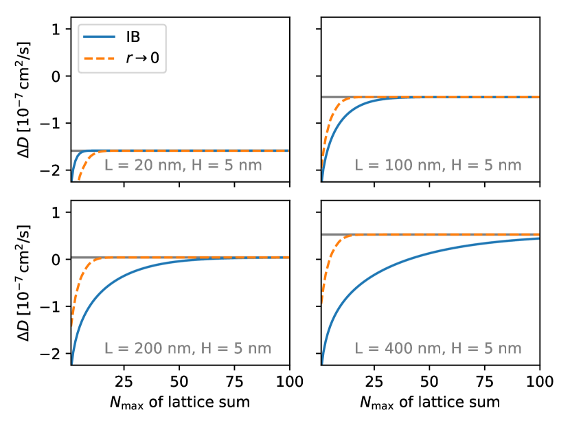
When calculating the lattice sums for the theoretical descriptions, care should be taken that convergence is reached. For the IB method, convergence depends on the box geometry while we can safely assume the sums in the point-perturbation method to be converged after 20-30 summands (Fig. S2).

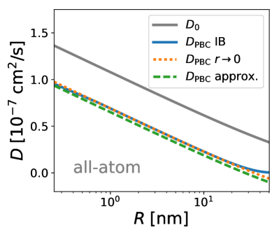
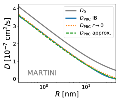
We calculated the radius dependence of those two theories and for the flat-box approximation (Eq. (2)) for typical values of fully atomistic and MARTINI coarse-grained simulations (Fig. S3).

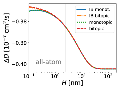
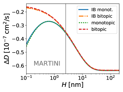
For the monotopic correction, we compare the descriptions around two typical regions of the interleaflet friction coefficient $b$ (Fig. S4). Typical values are for all-atom simulations ($b\approx 10^{8}\,\mathrm{Pa\,s/m}$) and for MARTINI ($b\approx 10^{6}-10^{7}\,\mathrm{Pa\,s/m}$) Camley et al. (2015).

Figure S2: Theoretical prediction of the difference $\Delta D=D_{\mathrm{PBC}}-D_{0}$ between the diffusion coefficients in PBC and in the infinite system depending on the number of summands (${n_{x}}^{2}+{n_{y}}^{2}\leq{N_{\mathrm{max}}}^{2}$) considered in the lattice sum for four different box geometries (constant $H=5\,\mathrm{nm}$ and $L=20$, 100, 200, and 400 nm) and a protein radius of $1\,\mathrm{nm}$. The differences were calculated for the Oseen correction (orange lines) evaluated using Eq. (S2) ($r\rightarrow 0$), and for the IB method (blue lines) using the difference of Eq. (S8) and Eq. (S9) (IB). The gray horizontal line shows the converged value.

Figure S3: Theoretical prediction of the diffusion coefficient of a cylindrical membrane inclusion as a function of its radius $R$ for different levels of theory for properties of typical all-atom (left) and MARTINI (right) simulations. Values for all-atom: $\eta_{f}=5.47\times 10^{-4}\;\mathrm{Pa\,s}$, $\eta_{m}=1.6\times 10^{-10}\;\mathrm{Pa\,s\,m}$. Values for MARTINI: $\eta_{f}=7.0\times 10^{-4}\;\mathrm{Pa\,s}$, $\eta_{m}=4.0\times 10^{-11}\;\mathrm{Pa\,s\,m}$. In both cases, $L=100\,\mathrm{nm}$ and $H=5\,\mathrm{nm}$. Results are shown for the Oseen correction (orange lines), the approximate Oseen correction Eq. (2) (green lines), and the IB method (blue lines). For reference, the gray lines show $D_{0}$ calculated from Eq. (S9). Both in the all-atom and MARTINI systems, the Oseen and IB corrections coincide almost perfectly. Diffusion coefficients in PBC were calculated according to Eq. (S8) (IB) and by adding to Eq. (S9) the corrections from Eq. (S2) ($r\rightarrow 0$) and Eq. (2) (flat-box approximation), respectively. The deviations shown for very small radii are caused by the slower convergence of the IB method (see Fig. S2).

I.4 Comparison of Monotopic and Transmembrane Correction

In comparisons for typical membrane physical parameters (such as in Fig. S4), we found the difference in the monotopic and transmembrane corrections to be negligible, especially for the high intermonolayer friction in atomistic simulations. Notable deviations are only observed for $b<10^{6}$ Pa s/m, a regime just below the one of MARTINI simulations. The weak dependence on the interleaflet friction coefficient $b$ renders it impossible to obtain $b$ from the size dependence. As an advantage, the use of the transmembrane (bitopic) correction and its flat-box approximation also for monotopic molecules simplifies the analysis.

For large heights, the monotopic and bitopic (transmembrane) expressions converge. For $H\rightarrow\infty$ and $k$ small but finite, we have for the reciprocal of the summand in the monotopic case: $(A^{2}(k)-B^{2}(k))/A(k)\approx 2\eta_{f}k+(\eta_{m}-\eta_{f}^{2}/b)k^{2}+\mathcal{O}(k^{3})$. For the bitopic case, we have exactly $2\eta_{f}k+\eta_{m}k^{2}$. That is, the two expressions have the same leading term and almost the same secondary term. The relative deviation of the factor of $k^{2}$ is therefore $\eta_{f}^{2}/(\eta_{m}b)\approx 1/40$. With MARTINI values, this means that also the $k^{2}$ term is essentially identical with only a 2.5 % correction. We therefore expect the bitopic correction to be sufficient in most cases and interpret the term $\eta_{f}^{2}/(\eta_{m}b)$ as the (dimensionless) relative importance of using the monotopic correction instead of the bitopic one. For our POPC simulations, we estimate an importance of $\eta_{f}^{2}/(\eta_{m}b)\approx 0.008$ for the monotopic correction from the results of the fit and from a value of $b=2.8\times 10^{6}$ Pa s/m. This value was estimated for a similar lipid in the MARTINI model, however with a longer saturated tail (five beads instead of four) and at 323 K den Otter and Shkulipa (2007), but we assume it provides a good estimate and we can use it to compare the two formalisms

In the monotopic IB and Oseen corrections for very small $H$, we noticed a turnover to a pathological divergence to $\Delta D\rightarrow-\infty$ (see Fig. S5). This small-$H$ divergence might be associated with the not strictly $z$-periodic formulation of the monotopic Oseen tensor Camley et al. (2015). It is difficult to test from our data gained in a $b$-insensitive regime whether the monotopic Oseen tensor describes the dynamics significantly better than the standard bitopic one.

Figure S4: Theoretical prediction of the diffusion coefficient of a cylindrical monotopic membrane inclusion with radius 0.5 nm as a function of interleaflet friction coefficient $b$ for properties of typical all-atom (left) and MARTINI (right) simulations. Values for all-atom: $\eta_{f}=5.47\times 10^{-4}\;\mathrm{Pa\,s}$, $\eta_{m}=1.6\times 10^{-10}\;\mathrm{Pa\,s\,m}$. Values for MARTINI: $\eta_{f}=7.0\times 10^{-4}\;\mathrm{Pa\,s}$, $\eta_{m}=4.0\times 10^{-11}\;\mathrm{Pa\,s\,m}$. In both cases, $L=100\,\mathrm{nm}$ and $H=5\,\mathrm{nm}$. Results are shown for the Oseen correction (orange lines), the approximate Oseen correction Eq. (2) (green lines), and the IB method (blue lines). For reference, the gray lines show $D_{0}$ calculated from Eq. (S11). Both in the all-atom and MARTINI systems, the Oseen and IB corrections coincide almost perfectly. Diffusion coefficients in PBC were calculated according to Eq. (S10) (IB) and by adding to Eq. (S11) the corrections from Eq. (S4) ($r\rightarrow 0$) and Eq. (2) (flat-box approximation), respectively.

Figure S5: Theoretical prediction of the difference $\Delta D=D_{\mathrm{PBC}}-D_{0}$ between the diffusion coefficients in PBC and in the infinite system for a cylindrical monotopic membrane inclusion with radius 0.5 nm as a function of $H$ for properties of typical all-atom (left) and MARTINI (right) simulations. Values for all-atom: $\eta_{f}=5.47\times 10^{-4}\;\mathrm{Pa\,s}$, $\eta_{m}=1.6\times 10^{-10}\;\mathrm{Pa\,s\,m}$, $b=1.0\times 10^{8}\;\mathrm{Pa\,s/m}$. Values for MARTINI: $\eta_{f}=7.0\times 10^{-4}\;\mathrm{Pa\,s}$, $\eta_{m}=4.0\times 10^{-11}\;\mathrm{Pa\,s\,m}$, $b=2.8\times 10^{6}\;\mathrm{Pa\,s/m}$. In both cases, $L=100\,\mathrm{nm}$. Results are shown for the Oseen correction (green lines for monotopic and red lines for bitopic) and the IB method (blue lines for monotopic and orange lines for bitopic). For large $H$, all corrections coincide almost perfectly. Vertical lines indicate a typical value in membrane simulations, $H=2.5$ nm.

II Simulation Details

II.1 Height Study

For our simulations of neat POPC membrane systems, we used the protocol and setup of Vögele and Hummer (2016), except for variations in box geometry. To fit the viscosities and the infinite-system diffusion coefficient, we used the simulation data from both studies. To give the context, we show the combined data in Fig. S6 and mean-squared displacement (MSD) curves of both studies in Fig. S7.

init. $L_{z}$ [nm]	num. of lipids	num. of water beads	box width $\langle L\rangle$ [nm]	box height $\langle L_{z}\rangle$ [nm]	sim. time [$\mathrm{\mu s}$]
9	540800	6791600	416.71(5)	9.43(1)	2.00
15	540800	14664800	417.02(1)	15.44(1)	2.00
22	540800	23850200	417.12(1)	22.44(1)	0.60
30	540800	34347800	417.17(1)	30.46(1)	2.00
40	540800	47469800	417.17(1)	40.50(1)	0.53
50	540800	60591800	417.20(1)	50.49(1)	2.00
75	540800	93396800	417.21(1)	75.51(1)	1.00
99	540800	124889600	417.19(1)	99.61(1)	0.50

Table S1: System parameters of the lipid membrane simulations to test the height dependence.

Figure S6: Diffusion coefficients in the full data set of POPC simulations with varied width (orange) at $H=2.25\,\mathrm{nm}$ and varied height (red) at $L=417\,\mathrm{nm}$, respectively, together with the corrected values and the best-fit infinite-system values (blue). The corresponding height dependence (here: red) for 417 nm is shown explicitly in Figure 1.

Figure S7: MSD curves for the height study (left) and, for comparison, from a width study (right) from earlier work Vögele and Hummer (2016). The upper plots show the initial phase and the lower the long-time behavior on a logarithmic scale with the fitting range in gray.

In a typical application, one would use the viscosity $\eta_{f}$ of the bulk solvent as input instead of performing a computationally expensive height study. Using $\eta_{f}=10.2$ Pa s (as obtained from pressure fluctuations in bulk-solvent simulations; see Table S3) in the analysis of only the flat-box simulations of Vögele and Hummer (2016), we obtained almost the same values of $D_{0}$ and $\eta_{m}$ for the POPC membrane as in the global fit that included the height-dependent simulations and left $\eta_{f}$ variable (main text). Results for the full Oseen correction Eq. (1) using bitopic and monotopic Oseen tensors, and for the approximate bitopic correction Eq. (2), are listed in Table S2. Also included are fits with fixed $\eta_{f}$ to all POPC membrane simulations here and in Vögele and Hummer (2016). The consistency of all fits justifies (1) fixing the solvent viscosity $\eta_{f}$ at a precalculated bulk value, and (2) using the approximate expression Eq. (2) for the analysis of typical membrane simulations.

data set	correction	$D_{0}$ [$10^{-7}$ cm2/s]	$\eta_{m}$ [10-11 Pa s m] ]
flat boxes	monotopic	6.20(2)	4.07(6)
flat boxes	bitopic	6.16(2)	3.94(6)
flat boxes	approximate	6.23(2)	3.92(6)
all data	monotopic	6.20(2)	4.06(6)
all data	bitopic	6.18(2)	3.96(6)
all data	approximate	6.20(2)	3.89(6)

Table S2: Infinite-system diffusion coefficient and membrane surface viscosity obtained from fits of the full Oseen correction Eq. (1) using monotopic and bitopic Oseen tensors, and of the approximate bitopic Oseen correction Eq. (2) at fixed fluid viscosity $\eta_{f}=10.2$ Pa s. For reference, a bitopic fit to all data with $\eta_{f}$ variable gave (main text) $D_{0}=6.20(2)\times 10^{-7}$ cm²/s and $\eta_{m}=3.97(6)\times 10^{-11}$ Pa s m

II.2 Viscosity of Water from Pressure Fluctuations

The viscosity of a specific water model under certain conditions can be obtained via the fluctuations of the off-diagonal elements of the pressure tensor in a simulation with constant box volume. We calculated $\eta_{f}$ according to the following Einstein relation Hess (2002):

$$\eta_{f} = \lim_{t\rightarrow\infty}\frac{1}{2}\frac{V}{k_{\mathrm{B}}T}\frac{\mathrm{d}}{\mathrm{d}t}\left\langle\left(\int_{t_{0}}^{t_{0}+t}P_{xz}(t^{\prime})\,\mathrm{d}t^{\prime}\right)^{2}\right\rangle_{t_{0}}$$ (S14)

where $V$ is the box volume, $P_{xz}$ is any off-diagonal element of the pressure tensor, and $t$ is the time.

We simulated cubes of 524880 MARTINI water beads (10% of which were antifreeze particles) for $1.0\;\mathrm{\mu s}$ at a fixed edge length of $40\,\mathrm{nm}$ with the same thermostat settings as in the respective membrane simulations. From these simulations, we obtained the values for the water viscosity by fitting the slope of the correlation function in Eq. (S14) over the time range 64 to 80 ns. For the temperatures and thermostats used in this work, we obtained the following MARTINI water viscosities:

• $10.2(4)\;\mathrm{Pa\,s}$ for $300\;\mathrm{K}$ with the Berendsen thermostat Berendsen et al. (1984) according to the simulation protocol in Vögele and Hummer (2016)

• $8.4(4)\;\mathrm{Pa\,s}$ for $310\,\mathrm{K}$ with the modified Berendsen thermostat for canonical sampling (Bussi-Donadio-Parrinello thermostat) Bussi et al. (2007) according to the simulation protocol in Hedger et al. (2016) for the ANT1 protein-loaded system

• $7.1(4)\;\mathrm{Pa\,s}$ for $323\;\mathrm{K}$ with the Bussi-Donadio-Parrinello thermostat Bussi et al. (2007) according to the simulation protocol in Ingólfsson et al. (2014) for the plasma membrane

II.3 Details on the Influence of the Water Viscosity

In the simulations testing the influence of the water viscosity, we varied the mass of the MARTINI water beads and left all other parameters the same. The viscosity of bulk water scales with the square root of the water mass $M$, $\eta_{f}(M)=(M/M_{0})^{1/2}\eta_{f}(M_{0})$. By contrast, we expect the surface viscosity $\eta_{m}$ to be relatively unaffected, such that $L_{\mathrm{SD}}\propto M^{-1/2}$ approximately. We performed four simulations using MARTINI water beads with masses of $M=M_{0}=72$ and $M=144$, 288 and 720 amu. The box height was $L_{z}=9$ nm, and the width $L=40$ nm.

Figure S8: MSD of POPC lipids (left) and membrane-spanning CNTs Vögele and Hummer (2016) (right) for different water viscosities in a box of size $L=40$ nm and $L_{z}=9$ nm. The viscosity $\eta_{f}$ of MARTINI water was varied by changing the mass of water particles from 72 amu to 144, 288, and 720 amu, respectively. The upper plots show the initial phase and the lower the long-time behavior on a logarithmic scale with the fitting range in gray.

$M\;\mathrm{[amu]}$	72	144	288	720
$\eta_{f}\;[\mathrm{10^{-4}\,Pa\,s}]$	$10.2(2)$	$14.4(2)$	$20.4(2)$	$32.2(2)$
$\Delta D/D_{0}$(POPC)	-12.5 %	-10.5 %	-8.1 %	-5.1 %
$\Delta D/D_{0}$(CNT)	-29.2 %	-25.1 %	-19.6 %	-11.9 %

Table S3: Details on the various water viscosities: Mass $M$ of the water beads, corresponding water viscosity $\eta_{f}$, and resulting corrections on the diffusion coefficient for lipids and the CNT.

W mass [amu]	num. of lipids	num. of water beads	box width $\langle L\rangle$ [nm]	box height $\langle L_{z}\rangle$ [nm]	sim. time [$\mathrm{\mu s}$]
72	5408	67916	41.69(5)	9.43(2)	2.00
144	5408	67916	41.69(5)	9.42(2)	2.00
288	5408	67916	41.69(5)	9.43(2)	2.00
720	5408	67916	41.70(5)	9.42(2)	2.00

Table S4: System parameters of the lipid membrane simulations to test the viscosity dependence.

II.4 Details of the Protein-Crowded Membrane

ANT1	POPC	POPE	Card.	solvent	box width $\langle L\rangle$ [nm]	box height $\langle L_{z}\rangle$ [nm]	sim. time [$\mathrm{\mu s}$]
1	220	160	20	6588	12.05(5)	10.19(9)	2.00
4	880	640	80	26332	24.10(5)	10.19(4)	2.00
9	1980	1440	180	59202	36.15(5)	10.18(3)	2.00
16	3520	2560	320	105440	48.20(5)	10.19(2)	2.00
25	5500	4000	500	164875	60.24(5)	10.20(2)	2.00
49	10780	7840	980	322812	84.34(5)	10.19(1)	2.00
100	22000	16000	2000	658400	120.48(6)	10.19(1)	2.00
225	49500	36000	4500	1480950	180.72(6)	10.19(1)	2.00
400	88000	64000	8000	2634800	240.96(6)	10.19(1)	2.00
625	137500	100000	12500	4111250	301.20(7)	10.18(1)	2.00
900	198000	144000	18000	5925600	361.45(8)	10.19(1)	2.00

Table S5: System parameters of the ANT1 simulations.

             Protein                                                      Cardiolipin (lower leaflet)
       POPC (upper leaflet)                                       POPC (lower leaflet)
       POPE (upper leaflet)                                       POPE (lower leaflet)

Figure S9: Diffusion coefficient of all components in the simulations of ANT1 proteins in a cardiolipin-containing POPC/POPE membrane with the infinite-system value fitted with fixed fluid viscosity $\eta_{f}=8.4\times 10^{-4}\,\mathrm{Pa\,s}$.

             Protein                                     Cardiolipin (lower leaflet)

       POPC (upper leaflet)                     POPC (lower leaflet)

       POPE (upper leaflet)                     POPE (lower leaflet)

Figure S10: MSD curves of all components in the simulations of ANT1 proteins in a cardiolipin-containing POPC/POPE membrane.

membrane	$\eta_{m}$	$D_{0}$
component	$[10^{-11}\,\mathrm{Pa\,s\,m}]$	$[10^{-7}\;\mathrm{cm^{2}/s}]$
Protein	4.08	2.15
Cardiolipin	4.30	4.34
POPC, outer	4.47	7.34
POPC, inner	4.42	6.24
POPE, outer	4.43	7.26
POPE, inner	4.35	6.09

Table S6: Membrane viscosity $\eta_{m}$ and infinite-system diffusion coefficients $D_{0}$ from individual fits using the approximation Eq. (2) for each component. The viscosity obtained from a global fit is $\eta_{m}=4.36\times 10^{-11}\;\mathrm{Pa\,s\,m}$. The results deviate by typically $\approx$ 2 % and maximally by 5 % from those obtained by using the full Oseen correction (see Table S7).

membrane	$\eta_{m}$ (monotopic)	$D_{0}$ (monotopic)	$\eta_{m}$ (bitopic)	$D_{0}$ (bitopic)
component	$[10^{-11}\,\mathrm{Pa\,s\,m}]$	$[10^{-7}\;\mathrm{cm^{2}/s}]$	$[10^{-11}\,\mathrm{Pa\,s\,m}]$	$[10^{-7}\;\mathrm{cm^{2}/s}]$
Protein	-	-	4.08	2.04
Cardiolipin	4.45	4.26	4.30	4.24
POPC, outer	4.61	7.26	4.47	7.24
POPC, inner	4.57	6.16	4.41	6.13
POPE, outer	4.57	7.17	4.43	7.16
POPE, inner	4.50	6.01	4.34	5.99

Table S7: Membrane viscosity $\eta_{m}$ and infinite-system diffusion coefficients $D_{0}$ from individual fits for each component using the Oseen correction Eq. (1) with the monotopic and the bitopic formalism, respectively. For the monotopic case, $b=2.9\times 10^{6}$ Pa s/m was used.

II.5 Details of the Plasma Membrane Model

mult.	num. of lipids	num. of solvent beads	box width $\langle L\rangle$ [nm]	box height $\langle L_{z}\rangle$ [nm]	sim. time [$\mathrm{\mu s}$]
1	28535	292306	71.39(6)	11.30(2)	2.00
4	114140	1169224	142.80(6)	11.29(1)	2.00
9	256815	2630754	214.20(2)	11.29(1)	1.70
16	456560	4676896	285.59(3)	11.30(1)	2.00

Table S8: System parameters of the plasma membrane simulations.

Figure S11: Comparisons of the results for the plasma membrane. Top: Deviations of the diffusion coefficients in the simulations from the respective infinite-system value (shaded colored lines) with their average (black circles) and the theoretical prediction (dashed line). Bottom: Relative errors of the diffusion coefficients of different lipid species depending on their infinite-system diffusion coefficient. Squares show the results of the largest system and circles those of the smallest system under study.

Figure S12: Diffusion coefficients for membrane components that remain in each leaflet (inner/outer) and for those that jump between both leaflets. Colors are assigned according to the lipid types present in each group. Present in the inner as well as in the outer leaflet are phosphatidylcholines (PC - blue), phosphatidylethanolamines (PE - orange), and sphingomyelins (SM - green). Present only in the outer leaflet are monosialotetrahexosylgangliosides (GM1/G1 - red), monosialodihexosylganglioside (GM3/G3 - purple), and lysophosphatidylcholines (LPC/C - brown). Present only in the outer leaflet are phosphatidylserines (PS - red), phosphatidylinositols (PI - purple), phosphatidic acids (PA - brown), and phosphatidylinositol(1-3)phosphates (PIP/P(1-3) - pink). Components that flip between leaflets are ceramides (CER/CE - red), diacylglycerols (DAG/DG - purple) and cholesterol (brown). The vertical grey lines indicate $L_{c}$, the box width at which the infinite-system value of the diffusion coefficient is reproduced.

Figure S13: Membrane viscosity $\eta_{m}$ obtained from fits to each single component of the model plasma membrane, grouped by leaflet (“both” indicates components that flip between the inner and outer leaflets).

leaflet	$\eta_{m,i}\;[10^{-11}\,\mathrm{Pa\,s\,m}]$
outer	$4.68$
inner	$4.84$
both	$4.47$
global	$4.73$

Table S9: Membrane viscosity $\eta_{m}$ from fits for each leaflet and for a global fit.

References

- Pluhackova and Böckmann (2015) K. Pluhackova and R. A. Böckmann, J. Phys. Condens. Matter 27, 323103 (2015).
- Ingólfsson et al. (2016) H. I. Ingólfsson, C. Arnarez, X. Periole, and S. J. Marrink, J. Cell Sci. 129, 257 (2016).
- Hedger et al. (2016) G. Hedger, S. L. Rouse, J. Domanski, M. Chavent, H. Koldsø, and M. S. P. Sansom, Biochem. 55, 6238 (2016).
- Duncan et al. (2017) A. L. Duncan, T. Reddy, H. Koldsø, J. Hélie, P. W. Fowler, M. Chavent, and M. S. P. Sansom, Sci. Rep. 7, 16647 (2017).
- Ingólfsson et al. (2014) H. I. Ingólfsson, M. N. Melo, F. J. V. Eerden, C. Arnarez, C. A. López, T. A. Wassenaar, X. Periole, A. H. D. Vries, D. P. Tieleman, and S. J. Marrink, J. Am. Chem. Soc. 136, 14554 (2014).
- Marrink et al. (2007) S. J. Marrink, H. J. Risselada, S. Yefimov, D. P. Tieleman, and A. H. D. Vries, J. Phys. Chem. B 111, 7812 (2007).
- Cooke et al. (2005) I. R. Cooke, K. Kremer, and M. Deserno, Phys. Rev. E 72, 011506 (2005).
- Izvekov and Voth (2005) S. Izvekov and G. A. Voth, J. Phys. Chem. B 109, 2469 (2005).
- Wassenaar et al. (2015) T. A. Wassenaar, H. I. Ingólfsson, R. A. Böckmann, D. P. Tieleman, and S. J. Marrink, J. Chem. Theory Comput. 11, 2144 (2015).
- Stansfeld et al. (2015) P. J. Stansfeld, J. E. Goose, M. Caffrey, E. P. Carpenter, J. L. Parker, S. Newstead, and M. S. Sansom, Structure 23, 1350 (2015).
- Wu et al. (2014) E. L. Wu, X. Cheng, S. Jo, H. Rui, K. C. Song, E. M. Dávila-Contreras, Y. Qi, J. Lee, V. Monje-Galvan, R. M. Venable, J. B. Klauda, and W. Im, J. Comput. Chem. 35, 1997 (2014).
- Koldsø et al. (2016) H. Koldsø, T. Reddy, P. W. Fowler, A. L. Duncan, and M. S. P. Sansom, J. Phys. Chem. B 120, 8873 (2016).
- Lyman et al. (2018) E. Lyman, C. Eggeling, and C.-L. Hsieh, bioRxiv (2018), https://doi.org/10.1101/292383.
- Camley et al. (2015) B. A. Camley, M. G. Lerner, R. W. Pastor, and F. L. H. Brown, J. Chem. Phys. 143, 243113 (2015).
- Vögele and Hummer (2016) M. Vögele and G. Hummer, J. Phys. Chem. B 120, 8722 (2016).
- Venable et al. (2017) R. M. Venable, H. I. Ingólfsson, M. G. Lerner, B. S. Perrin, B. A. Camley, S. J. Marrink, F. L. Brown, and R. W. Pastor, J. Phys. Chem. B 121, 3443 (2017).
- Yeh and Hummer (2004) I. C. Yeh and G. Hummer, J. Phys. Chem. B 108, 15873 (2004).
- Dünweg and Kremer (1993) B. Dünweg and K. Kremer, J. Chem. Phys. 99, 6983 (1993).
- Simonnin et al. (2017) P. Simonnin, B. Noetinger, C. Nieto-Draghi, V. Marry, and B. Rotenberg, J. Chem. Theory Comput. 13, 2881 (2017).
- Saffman and Delbrück (1975) P. G. Saffman and M. Delbrück, Proc. Natl. Acad. Sci. USA 72, 3111 (1975).
- Hughes et al. (1981) B. D. Hughes, B. A. Pailthorpe, and L. R. White, J. Fluid Mech. 110, 349 (1981).
- Petrov and Schwille (2008) E. P. Petrov and P. Schwille, Biophys. J. 94, L41 (2008).
- (23) See Supplemental Material for details about numerical evaluations, simulations, and water viscosity dependence.
- Hess et al. (2008) B. Hess, C. Kutzner, D. Van Der Spoel, and E. Lindahl, J. Chem. Theory Comput. 4, 435 (2008).
- Berendsen et al. (1984) H. J. C. Berendsen, J. P. M. Postma, W. F. van Gunsteren, A. DiNola, and J. R. Haak, J. Chem. Phys. 81, 3684 (1984).
- Bussi et al. (2007) G. Bussi, D. Donadio, and M. Parrinello, J. Chem. Phys. 126, 014101 (2007).
- Vögele et al. (2018) M. Vögele, J. Köfinger, and G. Hummer, Faraday Discuss. (2018), https://doi.org/10.1039/C8FD00011E, in press.
- Calandrini et al. (2011) V. Calandrini, E. Pellegrini, P. Calligari, K. Hinsen, and G. R. Kneller, Collection SFN 12, 201 (2011).
- Hess (2002) B. Hess, J. Chem. Phys. 116, 209 (2002).
- den Otter and Shkulipa (2007) W. den Otter and S. Shkulipa, Biophys. J. 93, 423 (2007).
- Javanainen et al. (2017) M. Javanainen, H. Martinez-Seara, R. Metzler, and I. Vattulainen, J. Phys. Chem. Lett. 8, 4308 (2017).
Supplemental Material: