Instability of precession driven Kelvin modes: Evidence of a detuning effect

Abstract

We report an experimental study of the instability of a nearly-resonant Kelvin mode forced by precession in a cylindrical vessel. The instability is detected above a critical precession ratio via the appearance of peaks in the temporal power spectrum of pressure fluctuations measured at the end-walls of the cylinder. The corresponding frequencies can be grouped into frequency sets satisfying resonance conditions with the forced Kelvin mode.

We show that one set forms a triad that is associated with a parametric resonance of Kelvin modes. We observe a significant frequency variation of the unstable modes with the precession ratio, which can be explained by a detuning mechanism due to the slowdown of the background flow. By introducing a semi-analytical model, we show that the departure of the flow from the solid body rotation leads to a modification of the dispersion relation of Kelvin modes and to a detuning of the resonance condition.

The second frequency set includes a very low frequency and does not exhibit the properties of a parametric resonance between Kelvin modes. Interestingly this frequency set always emerges before the occurence of the triadic resonances, i.e. at a lower precession ratio, which implies that it may correspond to a new type of instability. We discuss the relevance of an instability of a geostrophic mode described by Kerswell [J. Fluid Mech. 1999, 382, 283–306] although other mechanisms cannot be completely ruled out.

I Introduction

Since the original work of Kelvin (Thomson, 1880) it is known that rotating columns of fluid support helical modes composed of two inertial waves, which nowadays are called Kelvin modes. Experiments have shown that Kelvin modes can be directly forced in precessing or librating flows McEwan (1970) or by emulating tidal forcing Le Bars et al. (2015). Kelvin modes may also appear via an instability, as observed in the Lamb-Oseen vortex Fabre et al. (2006), or in a column of fluid that is elliptically deformed Kerswell (2002). Global stability analysis shows that a single directly forced Kelvin mode may become unstable via a parametric (triadic) resonance with two further free Kelvin modes Kerswell (1999), i.e. two modes that are not present before the onset of the instability. Whereas the linear mechanisms have been extensively studied, the experimental investigation of the non-linear evolution of the instability, which involves the saturation process, is still an open issue. Two scenarios, which may coexist, have been suggested to explain the final stage of the instability. First, saturation can be achieved by non-linear interactions between the unstable modes and small scale structures. This leads to an energy transfer from the linearly unstable modes to small scale dissipative structures Kerswell (1999). This mechanism can be intermittent, as observed by McEwan (McEwan, 1970) during the ”resonant collapse” of Kelvin modes. Saturation can also be achieved by a secondary mean flow generated directly by the unstable modes. The resulting modification of the background flow leads to a saturation of the amplitude of the unstable mode, via a frequency detuning or a phase shifting between the unstable modes and the forced mode Waleffe (1989). This problem can be decomposed into two parts: the modification of the background flow produced by Kelvin modes, and the feedback of this flow on the Kelvin modes. The first point is a complex problem because the direct non-linear interaction between a single Kelvin mode and the background flow is not permitted at first order for the steady case in the long time scale (Greenspan, 1969). However, the emergence of strong mean flows via non-linear interactions between inertial modes is allowed for finite Rossby number (the ratio between non-linear advection $|\textbf{u}\nabla\textbf{u}|$ over the Coriolis term $|2{\bm{\Omega}}\times\textbf{u}|$) or finite Ekmann number (the ratio between viscous forces and the Coriolis force) Le Reun et al. (2017).

In the present study we deal with the second point by examining experimentally and theoretically the detuning of resonant Kelvin modes caused by the induced modification of the background flow in a precessing fluid. The experiments utilize a cylinder filled with water which rotates around its symmetry axis at the rotation rate $\Omega_{\rm{c}}$. This cylinder is mounted on a turntable rotating at the precession rate $\Omega_{\rm{p}}$. When the angle between the axes of rotation and precession (the nutation angle $\alpha$) is non-zero, the flow deviates from the solid body rotation, due to the acceleration of the rotation axis. As originally observed by McEwan (McEwan, 1970), the primary response of the fluid is a laminar flow that is composed of Kelvin modes superimposed on a solid body rotation Manasseh (1992); Kobine (1995); Meunier et al. (2008); Liao and Zhang (2012). The gyroscopic force due to precession directly forces a Kelvin mode with azimuthal wave number $m=1$ and angular frequency $-\Omega_{\rm{c}}$ in the frame of reference of the cylinder. This mode can be resonant if its eigenfrequency $\omega$ is close to the angular frequency of the forcing $\Omega_{\rm{c}}$. Out of the resonance, the amplitude of the mode scales like $|\omega-\Omega_{\rm{c}}|^{-1}$ and increases with the strength of the precession, quantified by the precession ratio $\epsilon=\Omega_{\rm{p}}/\Omega_{\rm{c}}$. At resonance, viscous and non-linear effects must be taken into account for explaining the saturation of the forced Kelvin mode Gans (1970); Meunier et al. (2008); Kobine (1996); Liao and Zhang (2012). It is worth noting that non-linear and viscous effects may lead to the generation of a geostrophic mode Meunier et al. (2008); Kobine (1996) in the laminar regime before the occurrence of the instability of the forced Kelvin modes Kerswell (1999). The instability of the forced Kelvin mode sets in above a critical precession ratio McEwan (1970); Manasseh (1992); Kobine (1995), and the linear analyses Kerswell (1999) predicts a triggering of a parametric (triadic) resonance which has been confirmed in experimental and numerical studies Lagrange et al. (2008); Lin et al. (2014); Albrecht et al. (2015); Herault et al. (2015); Giesecke et al. (2015); Albrecht et al. (2018). The parametric instability can either saturate to a periodic state Lagrange et al. (2011) or trigger a non-stationary sequence of bifurcations which may account for a chaotic state called resonant collapse as it has been observed experimentally McEwan (1970); Manasseh (1992); Lin et al. (2014). The weakly non-linear analysis of the instability Lagrange et al. (2011) shows that saturation can also be achieved by a detuning of the forced Kelvin mode due to a modification of the solid body rotation.

This scenario is supported by measurements of the modification of the background flow in the laminar Kobine (1996); Meunier et al. (2008) as well as in the nonlinear regime Lagrange et al. (2011); Mouhali et al. (2012). In this regard, simulations and experiments indicate a fundamental difference between the emerging flow at small and at large nutation angle $\alpha$, which can be seen in the transition from laminar to turbulent flow. At small $\alpha$ different types of the transition into the turbulent regime can be observed, which are usually referred to as resonant collapse Manasseh (1992). Recent simulations by Albrecht et al. (2018) give evidence that a cascadic emergence of triadic resonances determines the transient evolution during the resonant collapse. In contrast, at large $\alpha$ only one type of definite transition is found at a critical precession ratio Herault et al. (2015) which presumably is not related to the first instabilities because it only occurs for a precession ratio approximately two times larger than the threshold of the parametric instability. Moreover, measurements from our previous study Herault et al. (2015) do not support the scenario of a resonant collapse of Kelvin modes but rather a subcritical transition with sudden and definitive relaminarizations, a phenomenon frequently observed in shear-flows Hof et al. (2006). A strong shear flow is indeed observed in our experiments and simulations which is reflected in a significant braking of the initial solid body rotation Giesecke et al. (2018). The associated strong velocity gradients near the outer walls tend to become unstable which may trigger the transition in the turbulent regime at large $\alpha$ by eruptions that originate in the lateral boundary layers and penetrate into the bulk flow Lopez and Marques (2016).

The generation of mean flows from precessional forcing is a rather complex process strongly impacted by nonlinearities, and the analytical calculation of the feedback of the instability, i.e. how the unstable modes backreact on the background flow, is hardly tractable, although particular studies have been applied to the laminar case for forced Kelvin modes Meunier et al. (2008) and to the unstable regime Lagrange et al. (2011). In this study, we do not focus on this part, but we assume a priori the functional form of the modified background flow which results from some unspecified mechanism. In particular, we do not assume that the instability is responsible for the modification of the background flow, but that a modified background flow impacts the instabilities by detuning, which finally causes the saturation of the instability.

Up to present, the experimental evidence of the saturation via a modification of the background flow that goes along with the detuning of Kelvin modes is still lacking. The detuning of the frequency of the forced mode could only be observed indirectly by measuring a decrease of its amplitude, because its frequency always remains the one of the forcing. In contrast, the detuning of free Kelvin modes can be measured directly because only the condition of resonance must be maintained, i.e. the difference or the sum of their frequencies. The present paper aims at demonstrating the detuning of free Kelvin modes with experimental measurements and complementary analytic calculations that are based on a perturbation approach. After introducing the experimental set-up and the theoretical background in sections II and III, we report our experimental observations in section IV. We briefly discuss the qualitative behavior of the pattern of the unstable Kelvin mode and study the amplitudes and the frequencies of the contributing modes. The remainder of the paper aims at an analytical explanation of the detuning of the frequency as a function of the modification of the background flow (Section V.1) followed by a brief sketch of the theoretical background that describes the impact of shear on the eigenmodes in a rotating fluid (Section V). Finally, we discuss the effect of the detuning on the parametric instability (section VI).

II Mathematical preliminaries

II.1 Basic equations

We consider a viscous and incompressible fluid with kinematic viscosity $\nu$, which is contained in a rigid cylindrical cavity of radius $R$ and height $H$. We apply cylindrical coordinates with the origin of the reference frame located at the center of the cylinder (Fig. 1b) so that the fluid domain is defined by $(r,\varphi,z)\in\left([0,R]\times[0,2\pi]\times[-H/2,H/2]\right)$. The cylinder rotates at an angular frequency $\Omega_{\rm{c}}=2\pi f_{\rm{c}}$ around the axial direction $\textbf{e}_{z}$. This axis $\textbf{e}_{z}$ in turn rotates around a second axis, the axis of precession $\textbf{e}_{\rm{p}}$, at the angular frequency $\Omega_{\rm{p}}=2\pi f_{\rm{p}}$. In the present study the angle between $\textbf{e}_{z}$ and $\textbf{e}_{\rm{p}}$ is fixed at $\alpha=90^{\circ}$. In the following, all computations are performed in the reference frame of the cylinder, where the walls are at rest. In this system, it is the axis of precession, $\textbf{e}_{\rm{p}}$, that rotates around the axis $\textbf{e}_{z}$. The equation describing the velocity field v in the cylinder reference frame rotating at ${\bm{\Omega}}=\Omega_{\rm{c}}\textbf{e}_{z}+\Omega_{\rm{p}}\textbf{e}_{\rm{p}}$ is

$$\partial_{t}\textbf{v}+\textbf{v}\cdot\nabla\textbf{v}+2\left[\Omega_{\rm{c}}\textbf{e}_{z}+\Omega_{\rm{p}}\textbf{e}_{\rm{p}}(t)\right]\times\textbf{v}=-\frac{1}{\rho}\nabla P+\textbf{F}+\nu\Delta\textbf{v}$$ (1)

where v additionally satisfies the mass conservation

$$\nabla\cdot\textbf{v}=0$$ (2)

and $\textbf{e}_{\rm{p}}(t)$ is given by

$$\textbf{e}_{\rm{p}}(t)=\sin\alpha\cos(\Omega_{\rm{c}}t+\varphi)\hat{\textbf{r}}-\sin\alpha\sin(\Omega_{\rm{c}}t+\varphi)\hat{\bm{\varphi}}+\cos\alpha\hat{\textbf{z}}.$$ (3)

In equation (1) $P$ denotes the modified pressure that includes the centrifugal contributions. The forcing term F, also called Poincaré acceleration, corresponds to the gyroscopic force which is responsible for the departure of the flow from the solid body rotation and is given by

$$\textbf{F}=-\Omega_{\rm{c}}\Omega_{\rm{p}}r\cos(\Omega_{\rm{c}}t+\varphi)\textbf{e}_{z}.$$ (4)

The velocity field v satisfies no-slip conditions at the wall ($r=R$ and $z=\pm H/2$)

$$\textbf{v}=\textbf{0}.$$ (5)

The variables are made dimensionless using the time scale $\Omega_{\rm{c}}^{-1}$ and the length scale $R$. The rescaled coordinates become $(r^{\prime},z^{\prime})=(r/R,z/R)$ and the time $t^{\prime}=t\Omega_{\rm{c}}$. The equation governing the dynamics of the dimensionless velocity field $\textbf{U}=\textbf{v}/(R\Omega_{\rm{c}})$ and pressure field $P^{\prime}=P/(\rho R^{2}\Omega_{\rm{c}}^{2})$ is then

$$\partial_{t^{\prime}}\textbf{U}+\textbf{U}\cdot\nabla\textbf{U}+2\left(\textbf{e}_{z}+\epsilon\textbf{e}_{\rm{p}}\right)\times\textbf{U}=-\nabla P^{\prime}+\textbf{F}^{\prime}+{\rm{Ek}}\Delta\textbf{U}$$ (6)

with $\epsilon=\Omega_{\rm{p}}/\Omega_{\rm{c}}$ the precession ratio and ${\rm{Ek}}=\nu/(\Omega_{\rm{c}}R^{2})$ the Ekman number. The forcing term is then given by

$$\textbf{F}^{\prime}=-\epsilon r\cos(t+\varphi)\textbf{e}_{z}.$$ (7)

For the sake of simplicity, we remove the prime index in the remainder of the paper. In the limit ${\rm{Ek}}\rightarrow 0$, the viscous effects are essentially localized in the Ekman boundary layers, varying with $\delta_{{\rm{Ek}}}\sim{\rm{Ek}}^{1/2}$. In this limit, the bulk flow satisfies only a no-outward flow condition close to the wall, by omitting the pumping at first order Greenspan (1968),

$$\textbf{U}\cdot\textbf{n}={0}\quad\hbox{at the wall}$$ (8)

with n the unitary vector normal to the wall.

II.2 Linearized equations

II.2.1 General case

In order to establish the dispersion relation of the eigenmodes of a rotating fluid in a cylinder (the Kelvin modes), we linearize the Navier–Stokes equation (6) by introducing the infinitesimal velocity perturbation $\textbf{u}=\textbf{U}-\textbf{U}_{\beta}$, where $\textbf{U}_{\beta}(r)$ is a mean azimuthal circulation that is given by $\textbf{U}_{\beta}=r\beta\Omega_{\beta}(r)\textbf{e}_{\varphi}$ with $\Omega_{\beta}(r)$ a continuous function of $r$ characterizing the departure from the solid body rotation and $\beta$ its real amplitude. Note that ${\Omega}_{\beta}$ only depends on the radius and is independent of $z$ (see section V). Note also that all calculations are performed in the cylinder reference frame, i.e., the frame co-rotating with the cylinder wall so that $\textbf{U}_{\beta}$ does not include the solid body rotation.

We linearize around $\textbf{U}_{\beta}(r)$ and neglect the non-linear term $\textbf{u}\cdot\nabla\textbf{u}$, the viscous term, the forcing term F and the non-stationary component of the Coriolis term $\epsilon\textbf{e}_{\rm{p}}{(t)}\times\textbf{u}$. The equation thus simplified describes the linear eigenmodes of a rotating fluid with a modified rotation profile in the limit of vanishing precession $\epsilon\rightarrow 0$ and reads

$$\left(\partial_{t}+\beta\Omega_{\beta}\partial_{\varphi}\right)\textbf{u}-2\beta\Omega_{\beta}u_{\varphi}\textbf{e}_{r}+\beta\Omega_{\beta}u_{r}\textbf{e}_{\varphi}+u_{r}\partial_{r}\textbf{U}_{\beta}+\textbf{e}_{z}\times\textbf{u}=-\nabla P.$$ (9)

We look for infinitesimal perturbations in the form of eigenmodes, characterized by an axial wave number $k$, an azimuthal wave number $m$ and a complex frequency $\omega$,

$$(\textbf{u},p)=\exp(i\omega t+im\varphi+ikz)\left(\begin{array}[]{rl}\tilde{u}_{r}(r)\\ \tilde{u}_{\varphi}(r)\\ \tilde{u}_{z}(r)\\ \tilde{p}(r)\\ \end{array}\right)+c.c$$ (10)

where $(\tilde{u}_{r},\tilde{u}_{\theta},\tilde{u}_{z},\tilde{p})$ are complex functions of $r$, and $c.c.$ refers to the complex conjugate in order to obtain a real velocity field. The eigenmodes satisfy the boundary condition (8) at the top and the bottom of the cylinder, $z=\pm\Gamma^{-1}/2$, if $k=\pi n\Gamma$ with $n$ an integer. The linearized equation with the given perturbations (10) leads to the following set of equations

$$\left\{\begin{array}[]{ll}\displaystyle{i\left(\omega+m\beta\Omega_{\beta}\right)\tilde{u}_{r}-2\left(1+\beta\Omega_{\beta}\right)\tilde{u}_{\varphi}+\partial_{r}\tilde{p}=0}\\ \\ \displaystyle{i\left(\omega+m\beta\Omega_{\beta}\right)\tilde{u}_{\varphi}+\left(2+\beta\zeta_{\beta}\right)\tilde{u}_{r}+\frac{im}{r}\tilde{p}=0}\\ \\ \displaystyle{i\left(\omega+m\beta\Omega_{\beta}\right)\tilde{u}_{z}+ik\tilde{p}=0}\\ \\ \displaystyle{\frac{1}{r}\partial_{r}(r\tilde{u}_{r})+\frac{im}{r}\tilde{u}_{\varphi}+ik\tilde{u}_{z}=0}\end{array}\right.$$ (11)

with $\zeta_{\beta}={{2}}\Omega_{\beta}+r\partial_{r}\Omega_{\beta}$ denoting the $z$ component of the vorticity associated to $\Omega_{\beta}$. The system of equations (11) can be rewritten using a four-component formulation for the complex velocity-pressure field $(\tilde{\textbf{u}},\tilde{p})$ which leads to the compact form

$$\left(i\omega{\mathcal{I}}+{\mathcal{L}}\right)(\tilde{\textbf{u}},\tilde{P})=\textbf{0},$$ (12)

with ${\mathcal{L}}={\mathcal{L}}_{0}+\beta{\mathcal{L}}_{\beta}$, and the operators $\mathcal{I}$, ${\mathcal{L}}_{0}$ and ${\mathcal{L}}_{\beta}$ given in appendix A.1. The operator ${\mathcal{L}}_{0}$ represents the action of the Coriolis force with the uniform rotation rate $\Omega_{\rm{c}}$ and the incompressibility condition, and ${\mathcal{L}}_{\beta}$ characterizes the effect of the modification of the background flow due to $\Omega_{\beta}(r)$.

II.2.2 Kelvin modes with uniform rotation

First, we consider the classical problem of a solid body rotation, i.e. $\beta=0$, which gives

$$\left(i\omega_{0l}{\mathcal{I}}+{\mathcal{L}}_{0}\right)(\tilde{\textbf{u}},\tilde{p})_{0l}=\textbf{0}$$ (13)

where the index $0$ is used to denote the eigenmodes and frequencies for $\beta=0$. The index $l$ denotes a radial eigenmode $(\tilde{\textbf{u}},\tilde{p})_{0l}$ with azimuthal and axial wave numbers $m$ and $k$ and characterizes the series of solutions of the dispersion relation (see next paragraph).

The corresponding dispersion relation provides the radial wave numbers $\delta_{0l}$ and frequencies $\omega_{0l}$ and consists of two equations given by

$$\omega_{0l}^{2}=\frac{4k^{2}}{\delta_{0l}^{2}+k^{2}}$$ (14)

and

$$(2+\omega_{0l})mJ_{m}(\delta_{0l})-\omega_{0l}\delta_{0l}J_{m+1}(\delta_{0l})=0$$ (15)

with $m$ and $k$ given and $J_{m}$ the Bessel function of order $m$. The first equation is the well known dispersion relation of inertial waves. The second equation results from the enforcement of the no-outflow condition $u_{r}=0$ at the lateral wall. For $m$ and $k$ fixed, there exists an infinitely countable number of couples $(\omega_{0l},\delta_{0l})$ satisfying equations (14) and (15). We distinguish three families of waves: Kelvin modes are either prograde with $\omega_{0l}/m<0$, rotating in the azimuthal direction of the background flow, or retrograde with $\omega_{0l}/m>0$, rotating in the opposite direction. For the retrograde (resp. prograde) Kelvin modes, the radial wave numbers $\delta_{0l}$ are numbered in ascending (resp. descending) order with $l$ a positive (negative) integer. The absolute value $|l|$ corresponds to the number of zeroes in the radial direction plus one (associated with the origin). The third family, called geostrophic modes, is characterized by $k=0$ and $\omega_{0l}=0$, and the radial wave number arises as a solution of $J_{m}(\delta_{0l})=0$.

Introducing the solution of Eq. (13) in (10) and imposing free-slip boundary conditions at the wall, the velocity field satisfying Eq. (9) is given by a sum of Kelvin modes

$$\textbf{u}(\textbf{r},t)=\sum_{m}\sum_{n}\sum_{l}\exp(i\omega_{0l}t+im\varphi)~{}a_{mnl}\textbf{u}_{mnl}(r,z)+c.c.$$ (16)

with $(r,\varphi,z)\in\left([0,1]\times[0,2\pi]\times[-\Gamma^{-1}/2,\Gamma^{-1}/2]\right)$. The complex amplitude of the Kelvin mode, $a_{[m,n,l]}$ with the wave numbers $m,n$ and $l$ is associated to the velocity components $\textbf{u}_{mnl}(r,z)$ given by

$$\textbf{u}_{mnl}(r,z)=\left(\begin{array}[]{rl}\tilde{u}^{r}_{mnl}(r)\sin(\pi n\Gamma z)\\[5.69046pt] \tilde{u}^{\varphi}_{mnl}(r)\sin(\pi n\Gamma z)\\[5.69046pt] \tilde{u}^{z}_{mnl}(r)\cos(\pi n\Gamma z)\end{array}\right)$$ (17)

and the radial structure of the Kelvin mode reads

$$\begin{array}[]{rcl}\displaystyle\tilde{u}^{r}_{mnl}(r)&=&\displaystyle{\frac{-i}{4-\omega_{0l}^{2}}\left(\frac{(2+\omega_{0l})m}{r}J_{m}(\delta_{0l}r)-\omega_{0l}\delta_{0l}J_{m+1}(\delta_{0l}r)\right)},\\ \\ \displaystyle\tilde{u}^{\varphi}_{mnl}(r)&=&\displaystyle{\frac{1}{4-\omega_{0l}^{2}}\left(\frac{(2+\omega_{0l})m}{r}J_{m}(\delta_{0l}r)-2\delta_{0l}J_{m+1}(\delta_{0l}r)\right)},\\ \\ \displaystyle\tilde{u}^{z}_{mnl}(r)&=&\displaystyle{-\frac{k}{\omega_{0l}}J_{m}(\delta_{0l}r)}.\end{array}$$ (23)

The velocity fields of the Kelvin modes form an orthogonal basis Greenspan (1968) for the scalar product

$$\int\limits_{r=0}^{1}\int\limits_{\varphi=0\vphantom{\Gamma}}^{2\pi}\int\limits_{z=-\nicefrac{{1}}{{2}}\Gamma}^{1/2\Gamma}\left(\textbf{u}_{mnl}(r,z)e^{im\varphi}\right)^{*}\cdot\left(\textbf{u}_{m^{\prime}n^{\prime}l^{\prime}}(r,z)e^{im^{\prime}\varphi}\right)rdrd\varphi dz=\frac{\pi}{\Gamma}e_{l^{\prime}l}\delta_{n^{\prime}n}\delta_{m^{\prime}m}$$ (24)

if they satisfy the boundary condition (8). The elements $e_{l^{\prime}l}$ (where we omit the indices $m$ and $n$ for the sake of brevity) on the right hand side of definition (24) are given by $e_{l^{\prime}l}=\langle\tilde{\textbf{u}}_{0l^{\prime}},\tilde{\textbf{u}}_{0l}\rangle\delta_{l^{\prime}l}$ $e_{l^{\prime}l}=\langle\tilde{\textbf{u}}_{l^{\prime}m^{\prime}n^{\prime}},\tilde{\textbf{u}}_{lmn}\rangle$ with

$$\langle\tilde{\textbf{u}}_{m^{\prime}n^{\prime}l^{\prime}},\tilde{\textbf{u}}_{mnl}\rangle=\int\limits_{r=0}^{1}\left[\tilde{u}^{r}_{m^{\prime}n^{\prime}l^{\prime}}{}^{*}\tilde{u}^{r}_{mnl}+\tilde{u}^{\varphi}_{m^{\prime}n^{\prime}l^{\prime}}{}^{*}\tilde{u}^{\varphi}_{mnl}+\tilde{u}^{z}_{m^{\prime}n^{\prime}l^{\prime}}{}^{*}\tilde{u}^{z}_{mnl}\right]rdr.$$ (25)

II.2.3 Laminar flow driven by precession

We briefly recall the response of a rotating fluid to precessional forcing. Two new terms appear due to precession: the Coriolis term associated with the axis $\textbf{e}_{\rm{p}}$, and the Poincaré acceleration caused by the temporal variation of $\textbf{e}_{z}$. Only the latter is usually considered at leading order which leads to the equation

$$\partial_{t}\textbf{u}+2\textbf{e}_{z}\times\textbf{u}+\nabla P=-\epsilon r\cos(t+\varphi)\textbf{e}_{z}.$$ (26)

We look for the solution as a sum of Kelvin modes of axial and radial wave numbers $n$ and $l$ forced at the frequency $\omega_{0l}=1$ and azimuthal wave number $m=1$ Manasseh (1994). In that case Eq. (16) becomes

$$\textbf{u}=\left(\sum_{n,l}a_{1nl}\textbf{u}_{1nl}(r,z)e^{it+i\varphi}\right)+c.c.$$ (27)

The gyroscopic force on the right hand side of equation (26) is anti-symmetric with respect to the mid-plane of the cylinder and only forces modes with an axial component with the same parity, i.e. with an odd axial wave number $n$. By using equation (13) and the properties of orthogonality (24), the amplitude $a_{[1,n,l]}$ is given by

$$a_{1nl}=-\frac{i}{1-\omega_{0l}}{{\frac{\Gamma}{\pi}}}\frac{\iiint\left(\textbf{u}_{1nl}e^{-(it+i\varphi)}\right)\cdot\textbf{F}\hbox{dV}}{\langle\tilde{\textbf{u}}_{mnl},\tilde{\textbf{u}}_{mnl}\rangle}$$ (28)

with $\omega_{0l}$ the eigenfrequency of the mode with $(m=1,n,l)$. The forcing term F (given by (7)) that appears beyond the Integral on the right side of (28) implies that the amplitude $a$ is directly proportional to the precession ratio $\epsilon$. An explicit calculation of the terms $a_{1nl}$ can be found in Meunier et al. (2008); Liao and Zhang (2012); Manasseh (1994). The forced mode is retrograde and standing in the turntable reference frame.

For $\Gamma=0.5$ the eigenfrequency of the mode $(m,n,l)=(1,1,1)$ is $\omega=0.996\Omega_{\rm{c}}$ so that our experimental configuration corresponds to a nearly-resonant case with a single forced Kelvin mode. Hence, we consider that the flow is mostly composed of one Kelvin mode plus the background flow before any instability. Near the resonance $\omega_{0l}\simeq 1$, the amplitude given by (28) diverges and viscous and non-linear effects must be considered for the computation of the amplitude of the Kelvin modes Gans (1970); Meunier et al. (2008); Liao and Zhang (2012).

III Experimental setup

The experimental setup is illustrated in Fig. 1a. The vessel is a cylinder of radius $R=163\,{\rm{mm}}$ and height $H=326\,{\rm{mm}}$ filled with water. For a qualitative visualization of the flow, a small amount of air is introduced so that the spatial distribution of small gas bubbles within the rotating vessel enables a first estimation of the basic structure of the flow. The bubbles are only used to visualize the flow pattern (reported in section IV.1) while all quantitative results presented in sections IV.2 and IV.3 have been obtained with a significantly smaller gas fraction. The container rotates around its symmetry axis with a frequency $f_{\rm{c}}$ of up to $10\,{\rm{Hz}}$ and is mounted on a turntable which can rotate with a frequency $f_{\rm{p}}$ of up to $1\,{\rm{Hz}}$. In all experiments discussed here the rotation axis and the precession axis are orthogonal ($\alpha=\pi/2$, Fig. 1b). A more detailed description of the experiment can be found in Herault et al. (2015).

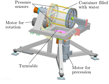
(a)

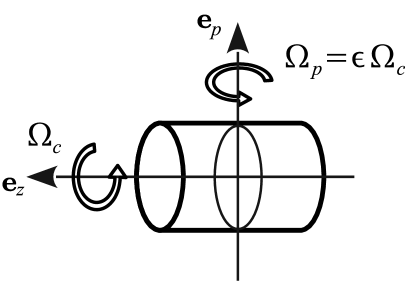
(b)

Figure 1: (a) Sketch of the experimental setup. (b) Sketch of the reference frame.

In the following, we will refer to angular frequencies defined by $\Omega_{\rm{c}}=2\pi f_{\rm{c}}$ and $\Omega_{\rm{p}}=2\pi f_{\rm{p}}$ in order to match the notation in the theory section below. The precessing system is now determined by three dimensionless parameters: the aspect ratio $\Gamma=R/H$ which in this study is always fixed at $\Gamma=0.5$, the Ekman number, ${\rm{Ek}}=\nu({\Omega}_{\rm{c}}R^{2})^{-1}$, and the precession ratio $\epsilon=\Omega_{\rm{p}}/\Omega_{\rm{c}}$. The mesured frequencies $\Omega$ ($\Omega_{\rm{c}}$ included) will be rescaled by $\Omega_{\rm{c}}$ so that $\Omega^{\prime}=\Omega/\Omega_{\rm{c}}$. To lighten the notations, we will omit the prime symbol in the next sections so that the angular frequency $\Omega=1$ corresponds to the angular frequency of the cylinder. The essential physical parameters that characterize the experimental set up are summarized in Table 1. Note that the reported Ekman numbers are one order of magnitude smaller than those obtained in previous studies Lagrange et al. (2008); Lin et al. (2014), which allows us to investigate less viscous regimes. In addition to the direct visualization of the flow, the pressure is measured at one of the end-caps close to the motor (Fig. 1a). Two XPM5 miniature pressure sensors with a diameter of $3.6\,{\rm{mm}}$ are mounted flush on one end-cap at a radius $r_{\rm{p}}=160\,{\rm{mm}}$ with an angle of $180^{\circ}$ between them. For these diametrically opposed probes, we define the symmetrical component $P_{\rm{s}}$ and the anti-symmetrical component $P_{\rm{a}}$ as the sum, respectively the difference, of their measurement values:

$$\left\{\begin{array}[]{ll}P_{\rm{s}}=\left[P(r_{\rm{p}},\varphi,H/2)+P(r_{\rm{p}},\varphi+\pi,H/2)\right]/2\\ \\ P_{\rm{a}}=\left[P(r_{\rm{p}},\varphi,H/2)-P(r_{\rm{p}},\varphi+\pi,H/2)\right]/2.\end{array}\right.$$ (29)

The power-spectral density (PSD) of $P_{\rm{s}}$ is given by

$$E_{\rm{s}}(\Omega)=\frac{1}{T_{\rm{m}}}\overline{\tilde{P}_{\rm{s}}(\Omega)\tilde{P}_{\rm{s}}^{*}{{(\Omega)}}}\quad\hbox{with}\quad\tilde{P}_{\rm{s}}{{(\Omega)}}=\int\limits_{0}^{T_{\rm{m}}}P_{\rm{s}}{{(t)}}e^{-i\Omega t}dt$$ (30)

with $T_{\rm{m}}$ the duration of the measurements and $\overline{~{}\cdot~{}}$ the average over the realizations. The same procedure defines the power-spectral density $E_{\rm{a}}$ of $P_{\rm{a}}$.

Table 1: Parameters and non-dimensional numbers used in this study. The Ekman number is based on a viscosity of water at $15^{\circ}\mbox{ C}$ of $\nu=1.17\times 10^{-6}\,{\rm{m}}^{2}/{\rm{s}}$.

Name	Notation	Definition	Experimental values
Cylinder frequency	$f_{\rm{c}}$	$-$	$0-10\,{\rm{Hz}}$
Precession frequency	$f_{\rm{p}}$	$-$	$0-1\,{\rm{Hz}}$
Radius	$R$	$-$	$163\,{\rm{mm}}$
Height	$H$	$-$	$326\,{\rm{mm}}$
Ekman number	${\rm{Ek}}$	$\nu(\Omega_{\rm{c}}R^{2})^{-1}$	$7\times 10^{-7}-7\times 10^{-6}$
Precession ratio	$\epsilon$	$f_{\rm{p}}/f_{\rm{c}}$	$2.5\times 10^{-2}-6\times 10^{-2}$
Aspect ratio	$\Gamma$	$R/H$	$0.5$

IV Experimental evidence of frequency detuning

IV.1 Flow pattern

(a)                                     (b)                                     (c)                                     (d)                                    

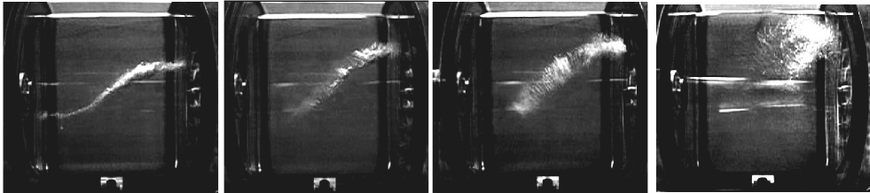
Figure 2: Photographs of the precessing cylinder in the turntable frame. The bright regions correspond to air bubbles, where the pressure is minimal. The Ekman number is ${\rm{Ek}}=7\times 10^{-7}$ ($f_{\rm{c}}=10\,{\rm{Hz}}$), and the precession ratio $\epsilon=0.74\times 10^{-2}$ (a), $\epsilon=3\times 10^{-2}$ (b), $\epsilon=3.4\times 10^{-2}$ (c) and $4.8\times 10^{-2}$ (d).

Before presenting quantitative results on the instability of the precessing flow, we discuss the qualitative diversity of the flow pattern for increasing precession ratio. We characterize the flow by analyzing the region of minimal pressure which is visualized by means of small air-bubbles that – at least in the laminar regime – align along the minimum pressure line. Although we do not observe any measurable changes of the instability thresholds in the experiments that include a small amount of gas, the air is removed to perform the quantitative measurement of the wall-pressure presented in the remainder of the paper. Figure 2 shows four snapshots of characteristic flow patterns at ${\rm{Ek}}=7\times 10^{-7}$ corresponding to $f_{\rm{c}}=10\,{\rm{Hz}}$. In the laminar regime the superposition of the nearly-resonant Kelvin mode and the solid body rotation yields an S-shaped tube that roughly corresponds to the effective rotation axis of the fluid ($\epsilon=0.74\times 10^{-2}$, Fig.  2a). The pattern is standing in the turntable frame, where the pictures are taken, and respects the centro-symmetry of the forcing. When the laminar flow becomes unstable around $\epsilon=3\times 10^{-2}$, we see erratic fluctuations resulting in a blurring of the S-tube (Fig. 2b). Further increasing $\epsilon$, the apparent width of the tube grows and we observe a stronger mixing in the vicinity of the tube associated to the spreading of bubbles (Fig. 2c). Around $\epsilon=4.8\times 10^{-2}$, the S-tube has dissolved and the bubbles are trapped in the upper-right region close to the end-cap (Fig. 2d). This localization of the bubbles close to one side can be explained by the appearance of one or few modes breaking the centro-symmetry of the laminar flow and thus creating a region of lower pressure close to one end-cap. At this state, the flow is chaotic but not yet turbulent. However, it is important to state that we never observe a phenomenon comparable to the resonant collapse Manasseh (1992) which would lead to an intermittent fine scale turbulence in the entire vessel. An abrupt transition to a turbulent state characterized by a homogeneous spreading of bubbles in the entire vessel only occurs above a critical precession ratio that is approximately twice as large as that for the onset of the instability. This phenomenon has been characterized in Herault et al. (2015) (see Fig 2 in Herault et al. (2015)) and will not be discussed in this study.

IV.2 Pressure measurement at constant Ekman number

IV.2.1 Frequencies

In the present section, we study the spectral information contained in the pressure measurements. The measurements are performed for constant Ekman number ${\rm{Ek}}=1.76\times 10^{-6}$ ($f_{\rm{c}}=4\,{\rm{Hz}}$) and the precession ratio $\epsilon$ is varied in the range $[0,6]\times 10^{-2}$. Each run lasts at least for $40$ minutes, or $9.6\times 10^{4}$ periods. In the following, time is measured in units of the rotation time of the cylinder so that all (angular) frequencies are denoted in units of the angular frequency of the cylinder, which, consistently, is set to unity, $\Omega_{\rm{c}}=1$. The power-spectra of the pressure components $P_{\rm{a}}$ (anti-symmetric) and $P_{\rm{s}}$ (symmetric), defined by equation (29), are shown in Fig. 3 for $\epsilon=0.68\times 10^{-2}$.

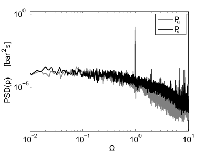
Figure 3: Spectra of the pressure components $P_{\rm{a}}$ (anti-symmetric, grey) and $P_{\rm{s}}$ (symmetric, black) for $\epsilon=0.68\times 10^{-2}$ and ${\rm{Ek}}=1.76\times 10^{-6}$ ($f_{\rm{c}}=4\mbox{ Hz}$, laminar regime).

In this case the flow is laminar and the spectrum is only composed of peaks located at $\Omega_{\rm{c}}$ and its multiples. The most intense peak belongs to the anti-symmetric component $P_{\rm{a}}$ at $\Omega_{\rm{c}}$ and originates from the forced Kelvin mode with $m=1$. Increasing the precession ratio to $\epsilon=3\times 10^{-2}$ the power spectra exhibit new features (Fig. 4a and b). An intense peak appears at low frequency at $\Omega_{1}=0.021$ (Fig. 4a). The smaller peak on the right side of $\Omega_{1}$ corresponds to the frequency $2\Omega_{1}$ and disappears for larger $\epsilon$. A close inspection of the power spectrum in the vicinity of $\Omega_{\rm{c}}=1$ shows the presence of two further peaks located on both sides of the forced mode $\Omega_{\rm{c}}$ (Fig. 4b). The maxima of these peaks correspond to the frequencies $\Omega_{4}=0.981$ and $\Omega_{5}=1.025$ (the choice for the index $4$ and $5$ is explained in next paragraph). The four frequencies $\Omega_{\rm{c}},\Omega_{1},\Omega_{4}$ and $\Omega_{5}$ fulfil the relations

$$\left\{\begin{array}[]{l}{{\Omega}}_{4}+{{\Omega}}_{1}\simeq{{\Omega}}_{\rm{c}}=1\\ \\ {{\Omega}}_{5}-{{\Omega}}_{1}\simeq{{\Omega}}_{\rm{c}}=1.\end{array}\right.$$ (31)

The location of the frequencies $\Omega_{1},\Omega_{4},$ and $\Omega_{5}$ depends monotonously on the precession ratio such that they always fulfill the relations (31).

Further increasing the precession ratio we find another pair of signals emerging at $\epsilon=3.75\times 10^{-2}$ (Fig. 5). At the lower end of the spectrum we now see two peaks at $\Omega_{1}\approx 0.064$ and $\Omega_{2}\approx 0.187$ (Fig. 5a) and three peaks in the vicinity of ${{\Omega}}_{\rm{c}}$ with ${{\Omega}}_{3}\approx 0.81$, $\Omega_{4}\approx 0.94$ and $\Omega_{5}\approx 1.06$. Comparable to the already known frequencies ${{\Omega}}_{1},{{\Omega}}_{4},{{\Omega}}_{5}$ the frequencies $\Omega_{2}$ and $\Omega_{3}$ fulfil the relation

$$\Omega_{2}+\Omega_{3} \simeq \Omega_{\rm{c}}=1.$$ (32)

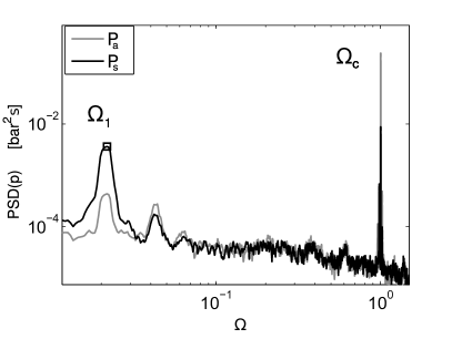
(a)

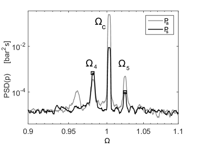
(b)

Figure 4: (a) Spectra of the pressure components $P_{\rm{a}}$ (anti-symmetric,grey) and $P_{\rm{s}}$ (symmetric, black) for $\epsilon=3\times 10^{-2}$ above the onset of instability. (b) Zoom in the vicinity of the forced mode ($\Omega_{\rm{c}}$). Three peaks in addition to the forced mode are well identified and labelled by $\Omega_{1},\Omega_{4}$ and $\Omega_{5}$.

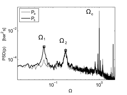
(a)

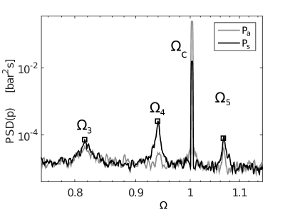
(b)

Figure 5: (a) Spectra of the pressure components $P_{\rm{a}}$ (anti-symmetric, grey) and $P_{\rm{s}}$ (symmetric, black) for $\epsilon=3.75\times 10^{-2}$ and ${\rm{Ek}}=1.77\times 10^{-6}$ past the onset of the instability. (b) Zoom in the vicinity of ${{\Omega}}={{\Omega}}_{\rm{c}}$. Beside the forced mode ${{\Omega}}_{\rm{c}}$ five peaks are well identified labeled by ${{\Omega}}_{1},{{\Omega}}_{2},{{\Omega}}_{3},{{\Omega}}_{4}$ and ${{\Omega}}_{5}$.

In total, there are now five frequencies indexed in an ascending order from $1$ to $5$, that can be grouped into two frequency sets $({{\Omega}}_{1},\Omega_{4},\Omega_{5})$ and $(\Omega_{2},\Omega_{3})$ satisfying (31) and (32), respectively. All frequencies show a systematic dependence on the precession ratio $\epsilon$ shown in Fig. 6 which presents the frequencies, $\Omega_{1}$ (circles), $\Omega_{2}$ (diamonds), $\Omega_{3}$ (triangles), $\Omega_{4}$ (squares) and $\Omega_{5}$ (stars) as a function of $\epsilon$. The relations (31) and  (32) between different pairs of the observed frequencies and the forcing frequency $\Omega_{\rm{c}}$ persist for all precession ratios (Fig. 7).

The remaining small differences, mostly smaller than $1\%$, are of the order of the control accuracy of the rotation rate of the motors. The individual signals occur only in a limited range of precession ratios with the frequencies $\Omega_{1},\Omega_{4}$ and $\Omega_{5}$ (respectively $\Omega_{2}$ and $\Omega_{3}$) appearing at $\epsilon=2.85\times 10^{-2}$ (resp. $3.34\times 10^{-2}$) and disappearing at $5.5\times 10^{-2}$ (resp. $4.2\times 10^{-2}$). The systematic study of the power-spectra shows that the frequencies vary monotonically with $\epsilon$, i.e. the frequencies $\Omega_{1},\Omega_{3}$ and $\Omega_{5}$ increase with the precession ratio, whereas $\Omega_{2}$ and $\Omega_{4}$ decrease. We further observe a qualitative change in the behavior of the frequency variations. Initially, for $\epsilon<\epsilon^{*}\approx 4.3\times 10^{-2}$, the frequencies $\Omega_{1},\Omega_{4}$ and $\Omega_{5}$ exhibit a basically linear variation with $\epsilon$ which, e.g. for $\Omega_{1}$ can be described by

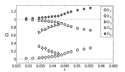
(a)

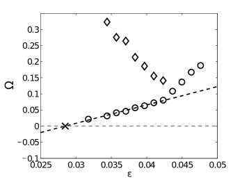
(b)

Figure 6: (a) Frequencies as a function of $\epsilon$ for ${\rm{Ek}}=1.76\times 10^{-6}$ ($f_{\rm{c}}=4\,{\rm{Hz}}$). The frequencies are sorted in an ascending order from the smallest ($\Omega_{1}$) to the largest ($\Omega_{5}$). (b) Zoom on the two smallest frequencies $\Omega_{1}$ and $\Omega_{2}$. Below $\epsilon^{*}=4.3\times 10^{-2}$ the frequency $\Omega_{1}$ follows a linear curve with $\Omega_{1}=C_{\rm{f}}(\epsilon-\epsilon_{\rm{c}})$. The black cross corresponds to the estimated threshold $\epsilon_{\rm{c}}=2.85\times 10^{-2}$.

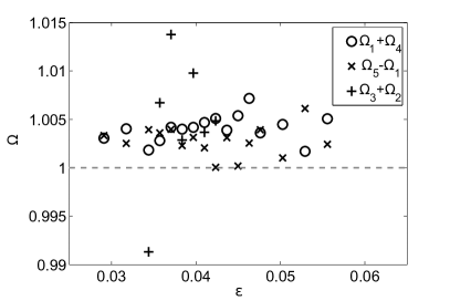
Figure 7: The resonance conditions with $\Omega_{1}+\Omega_{4}$ (circles), $\Omega_{5}-\Omega_{1}$ (crosses) and $\Omega_{2}+\Omega_{3}$ (plus) rescaled by $\Omega_{c}$.

$${{\Omega}}_{1}=C_{f}\left(\epsilon-\epsilon_{c}\right)$$ (33)

with $\epsilon_{c}=2.85\times 10^{-2}$ and $C_{f}=5.7$ (see dashed line in Fig. 6b). Similar relations can be given for ${{\Omega}}_{4}$ and ${{\Omega}}_{5}$, since ${{\Omega}}_{4,5}\pm{{\Omega}}_{1}\simeq 1$. We interpretate the coefficient $\epsilon_{c}$ as the threshold of the instability, by assuming that $\Omega_{1}$ departs from zero at the onset of the instability. For $\epsilon>\epsilon^{*}\simeq 4.3\times 10^{-2}$, $\Omega_{1},$ $\Omega_{4}$ and $\Omega_{5}$ abruptly change their slope which may be associated to a new instability. Note that the signals corresponding to $\Omega_{2}$ and $\Omega_{3}$ approximately vanish close to $\epsilon^{*}$. The evolution of the frequencies suggests that the disappearance of ${{\Omega}}_{2}$ and $\Omega_{3}$ occurs when the frequencies $\Omega_{1}$ and $\Omega_{2}$ are almost equal at $\epsilon^{*}$. However, measurements at $f_{\rm{c}}=1\,{\rm{Hz}}$ and $f_{\rm{c}}=8\,{\rm{Hz}}$ show that the frequency $\Omega_{2}$ only disappears slightly after the intersection with $\Omega_{1}$ (see e.g. red and green symbols in Fig. 8 below).

IV.3 Effect of the Ekman number

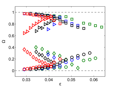
(a)

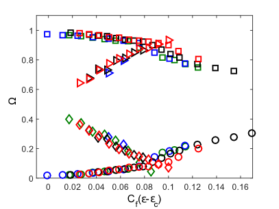
(b)

Figure 8: (a) Evolution of the rescaled frequencies $\Omega_{i}$ as a function of $\epsilon$ for $\Omega_{\rm{c}}=1\,{\rm{Hz}}$ (green), $2\,{\rm{Hz}}$ (blue), $4\,{\rm{Hz}}$ (black) and $8\,{\rm{Hz}}$ (red). (b) The same frequencies with a rescaled abscissa $C_{f}(\epsilon-\epsilon_{\rm{c}})$. In both plots $\Omega_{1}$ is denoted by circles, $\Omega_{2}$ by diamonds, $\Omega_{3}$ by triangles, and $\Omega_{4}$ by squares.

We have performed four series of measurements for different ${\rm{Ek}}=7\times 10^{-6}$, $3.5\times 10^{-6}$, $1.76\times 10^{-6}$ and $8.8\times 10^{-7}$ that correspond to rotation frequencies $f_{\rm{c}}=1$, $2$ , $4$ and $8\,{\rm{Hz}}$. The results are shown in Fig. 8a with $f_{\rm{c}}=1\,{\rm{Hz}}$ (green), $2\,{\rm{Hz}}$ (blue), $4\,{\rm{Hz}}$ (black) and $8\,{\rm{Hz}}$ (red). For the sake of clarity, we omit the frequencies $\Omega_{5}$. In all cases the power spectra show a behavior similar to the results presented in the previous section. Basically, we find up to five different peaks that globally exhibit the same tendency, but their thresholds of appearance and disappearance and their slope vary with the Ekman number. Generally, the frequencies appear for lower $\epsilon$, when ${\rm{Ek}}$ is decreased. Moreover, the frequencies $\Omega_{1}$, $\Omega_{4}$ and $\Omega_{5}$ always appear before $\Omega_{2}$ and $\Omega_{3}$.

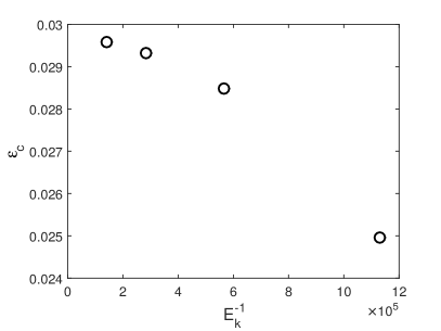
(a)

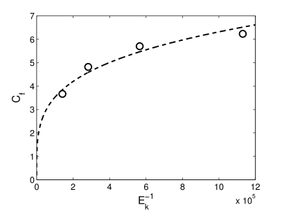
(b)

Figure 9: Evolution of the threshold $\epsilon_{\rm{c}}$ for the appearance of the mode $\Omega_{1}$ (a) and the coefficient $C_{{f}}$ (b) as a function of the inverse of the Ekman number ${\rm{Ek}}^{-1}$. The coefficient $C_{{f}}$ follows a power-law ${\rm{Ek}}^{-1/4}$.

In search for a common explanation of the underlying physical behavior, we change the variables: $({\rm{Ek}},\epsilon)\rightarrow C_{f}(\epsilon-\epsilon_{c})$ with $C_{f}({\rm{Ek}})$ and the critical value $\epsilon_{\rm{c}}({\rm{Ek}})$ for the onset of the instability. The frequencies are shown on Fig. 8b as a function of $C_{f}(\epsilon-\epsilon_{\rm{c}})$ with $C_{f}$ and $\epsilon_{\rm{c}}$ calculated separately for each Ekman number. In that case, all curves belonging to the frequencies $\Omega_{1},\Omega_{2},\Omega_{3},$ and $\Omega_{4}$, respectively, collapse, which was expected for $\Omega_{1}$ and $\Omega_{4}$ because $\Omega_{1}$ is used for the calculation of $\epsilon_{\rm{c}}$. However, it is surprising that the frequencies $\Omega_{2}$ and $\Omega_{3}$ scale in the same way. This strongly suggests that the variation of the frequencies is controlled by the same process, even if the nature of the instability may differ between both sets (see section IV.4 and VI). The threshold $\epsilon_{\rm{c}}$ decreases when ${\rm{Ek}}$ decreases, i.e. when $\Omega_{\rm{c}}$ increases, which goes along with the reduction of dissipative effects (Fig. 9a). The coefficient $C_{f}$ increases with the inverse of ${\rm{Ek}}$ and an empirical fitting indicates a scaling proportional to ${\rm{Ek}}^{-1/4}$ (Fig. 9b) so that for a constant relative precession ratio $\epsilon-\epsilon_{c}$ the detuning becomes stronger when the dissipation is reduced. Hence, we rule out the possibility of viscous detuning, which should increase with ${\rm{Ek}}$, and imply that the observed modification of all frequencies is provoked by a change of the base flow. For a constant relative precession ratio $\epsilon-\epsilon_{c}$ we further conclude that the detuning becomes stronger when the dissipation is reduced, which again rules out viscous detuning, which is expected to be constant for a given Ekman number Kerswell and Barenghi (1995).

IV.4 A preliminary analysis of the experimental results

The first step is to identify the modes from the dispersion relation Lagrange et al. (2011); Lin et al. (2014). One cannot expect a perfect correspondence between the frequencies given by the dispersion relation (14) and (15) and the experimental frequencies because the experimental ones vary with the precession ratio $\epsilon$. Here, we assume that at the threshold of appearance the frequencies $\Omega_{2}$ and $\Omega_{3}$ are close to exact solutions of the dispersion relation (14) and (15), i.e., the frequencies $\omega_{2}$ and $\omega_{3}$ of Kelvin modes with solid body rotation. This relies on the hypothesis that the variation of the frequencies is a consequence of the non-linear saturation of the instability Lagrange et al. (2011). Hence, we expect that the smaller the distance from the threshold, the weaker is the detuning.

Despite the fact that pressure measurements do not give information about the spatial structure of the modes it is suggestive to associate the measured frequencies $\Omega_{2}$ and $\Omega_{3}$, which at the threshold have the values $\Omega_{2}=0.37$ and $\Omega_{3}=0.64$, to Kelvin modes with the wave numbers given by $(m_{2},n_{2},l_{2})=(5,1,-1)$ and $(m_{3},n_{3},l_{3})=(6,2,1)$. According to the dispersion relation (14) and (15) the corresponding eigenfrequencies have the values $\omega_{2}=-0.34$ and $\omega_{3}=0.63$ so that the mode $\omega_{2}$ is prograde and the mode $\omega_{3}$ is retrograde. These solutions have the simplest possible geometric structure, i.e., the smallest azimuthal and axial wave numbers that satisfy the spatial resonance conditions (see equation (44) and (45) below and Meunier et al. (2008)). Similar Kelvin modes have also been identified in experiments conducted by Lagrange et al. (2008) even for aspect ratios that do not fullfil the resonance condition of the forced Kelvin mode $(m,n,l)=(1,1,1)$ and the corresponding triadic resonance turns out to be the most unstable combination Lagrange et al. (2011).

In contrast, a parametric resonance of free Kelvin modes with the frequencies $\Omega_{1}$ and $\Omega_{4}$ or $\Omega_{1}$ and $\Omega_{5}$ is not very likely. This can be seen, if we tentatively assume that the frequencies $\Omega_{1},\Omega_{4}$ and $\Omega_{5}$ are associated with Kelvin modes such that their frequencies at their threshold of appearance is given by the dispersion relation (14) and (15). The frequency $\Omega_{1}$ is almost equal to zero with $\Omega_{1}\simeq 0.025$ as the smallest value. Conversely, the frequencies $\Omega_{4}$ and $\Omega_{5}$ are almost equal to $1$, with $\Omega_{4}<1$ and $\Omega_{5}>1$. Certainly such solutions are allowed from the dispersion relation, however, these “extreme” cases go along with specific requirements for the radial wave number $\delta$ and the axial wave number $k$. In the limit of a vanishing frequency $\omega\rightarrow 0$ the dispersion relation (14) and (15) immediately yields $\delta\gg k$, whereas on the other side the limit $\omega\rightarrow 1$ would come along with $\delta\rightarrow\sqrt{3}k$. Additionally, the occurrence of a triadic resonance of two free Kelvin modes with $\omega\rightarrow 0$ and $\omega\rightarrow 1$ involving the directly forced mode further constrains the axial wave number $k$ by demanding $|\Delta k|=|k_{1}-k_{4}|=\pi\Gamma$ (which is the axial wave number of the forced mode), which, if both modes were free Kelvin modes, would end up with $\delta_{1}\gg\delta_{4}$ as a necessary condition for the radial wave numbers.

Consequently, if the modes $\Omega_{1}$ and $\Omega_{4}$ were free Kelvin modes, they would have significant different radial wave numbers with $\delta_{1}\gg\delta_{4}$ (The same argument works for the mode $\Omega_{5}$). The coupling between Kelvin modes with a large difference of radial wave number is in principle possible, but the efficiency of the coupling is very weak, and usually only parametric resonances with $\delta_{1}\simeq\delta_{4}$ are observed Kerswell (1999); Lagrange et al. (2008). Moreover, a mode with a large radial number is expected to be strongly damped by viscous effects, inhibiting the instability. Thus, we conclude that the frequencies $\Omega_{1},\Omega_{4},$ and $\Omega_{5}$ are very unlikely to be the spectral signature of a triadic resonance between a forced Kelvin mode and two free Kelvin modes. Instead we propose a new kind of instability Lagrange et al. (2008); Lin et al. (2014); Albrecht et al. (2015); Herault et al. (2015); Giesecke et al. (2015). where $\Omega_{1}$ is associated with a geostrophic mode ($k=0$) that results from the destabilisation of the (azimuthal) background flow. There are a couple of (experimentally justified) reasons for our interpretation. In case of a solid body rotation, a geostrophic mode must be steady in the cylinder reference frame, i.e. $\omega=0$. However, when the background flow departs from the solid body rotation, so that the background vorticity depends on the radius $r$, geostrophic modes are expected to be unsteady. The canonic example is a Rossby wave which has an angular frequency given by $\omega-kU\propto\beta$ where $\beta$ is the shear amplitude. In the same manner, the frequency of a non-axisymmetric geostrophic mode in the cylinder reference frame should increase with the shear amplitude $\beta$, as shown in Eq. (35) below.

Kerswell (1999) has reported the presence of an instability with a dominant geostrophic component, which displays some similarities with the features of the frequency set $(\Omega_{1},\Omega_{4},\Omega_{5})$. In his model, the modes do not emerge from a triad-type instability and the instability of the forced mode involves three further participants: a dominant geostrophic mode and two sub-dominant Kelvin modes with frequencies that are not solutions of the dispersion relation. These modes emerge from non-linear interactions between the geostrophic mode and the forced mode and their frequencies result from the linear combination of those two modes. Hence, the frequencies $\Omega_{4}$ and $\Omega_{5}$ belong to modes that are forced out of resonance, explaining the apparent mismatch between the observed frequency and their genuine eigenfrequency. Furthermore, Kerswell Kerswell (1999) found that this instability emerges before the parametric resonance, if the resonant triad is imperfectly tuned and the amplitude of the forced mode is relatively large. Since both conditions are satisfied in our experiment, this scenario may explain the presence of the frequency group $(\Omega_{1},\Omega_{4},\Omega_{5})$ before the frequency set associated with the parametric resonance $(\Omega_{2},\Omega_{3})$.

An alternative explanation for the low frequency mode $\Omega_{1}$ could be a secondary or tertiary instability of the triadic parametric resonance as they have been found experimentally by Lagrange et al. (2008, 2011) and numerically by Marques and Lopez (2015). In these cases the low frequency mode results from a slow drift in phase space between the forced mode and the two free Kelvin modes with $m=5$ and $m=6$, thus reflecting a slow near-heteroclinic cycle. However, these low frequency modes have only been found in a narrow region of parameter space so that most probably we can rule out this interpretation for our measurements, because we always observe $\Omega_{1}$ in a wide region of the parameter space $({\rm{Ek}},\epsilon)$ before (and thus it rules out a secondary instability) and after the occurrence of $\Omega_{2}$ and $\Omega_{3}$ due to the parametric resonances. Recently, Lopez and Marques Lopez and Marques (2018) found a low frequency state for a wider range of rotation frequencies (keeping ${\rm{Po}}$ fixed). However, due to their small nutation angle $\alpha=3^{\rm{\circ}}$, precession and rotation frequency cannot be independently controlled and the aspect ratrio $\Gamma=1.333$ used in their study entails quite different resonance frequencies, making a direct comparison rather difficult.

Nevertheless, the presence of a geostrophic mode and the associated instability remains speculative, and further measurements would be needed to confirm our hypothesis.

V Theoretical Model of parametric resonances in rotating flows with shear

V.1 Motivation and background flow

In the following, we will discuss the effect of the frequency detuning on the parametric resonance between Kelvin modes. We focus on the modes with the frequencies $\Omega_{2}$ and $\Omega_{3}$ which we previously associated with Kelvin modes with $(m_{2},n_{2},l_{2})=(5,1,-1)$ and $(m_{3},n_{3},l_{3})=(6,2,1)$, and we aim at explaining the detuning of $\Omega_{2}$ and $\Omega_{3}$ and the disappearance of the resonant triad in the same framework. We derive a model that gives the variation of the frequencies (i.e. the solutions of Eqs. (14) and (15)) with the amplitude of the modification of the background shear flow.

First, we address the form of the modification of the background flow, which we fix a priori since our measurements give no direct information about this secondary flow. We consider an axisymmetric stationary azimuthal perturbation $\beta U_{\beta}(r)=\beta r\Omega_{\beta}(r)$ in the cylinder frame with $0<\beta<1$, the amplitude of the secondary flow. Evidently, this flow cannot satisfy no-slip boundary conditions at the end-caps. We consider $V_{\beta}=0$ at the lateral wall at $r=1$ and we assume that a boundary layer exists between the end-caps and this flow. We choose a quadratic form for $\Omega_{\beta}$ given by

$$\Omega_{\beta}(r)=r^{2}-1$$ (35)

which corresponds to a retrograde flow for $\beta>0$. This functional form is the first possible polynomial correction to the rotation rate because any monomials $r^{n}$ with $n$ odd must vanish in order to satisfy the axi-symmetry. It also corresponds to the Chebyshev polynomial of the first kind $T_{2}(r)=r^{2}-1$ for $r\in[0,1]$. Interestingly, Meunier et al. Meunier et al. (2008) have observed a geostrophic mode (see their Fig. 17a) with a similar structure for the laminar regime with a forced Kelvin mode with $m=1$ and $l=1$ close its resonance.

The associated $z$-component of the vorticity is given by $\zeta_{\beta}={{2}}\Omega_{\beta}+r\partial_{r}\Omega_{\beta}=4r^{2}-2$. This flow is stable against centrifugal and shear-induced instabilities Chandrasekhar (1961). Figure 10 shows three paradigmatic azimuthal velocity profiles for $\beta=0$, $0.1$ and $0.25$.

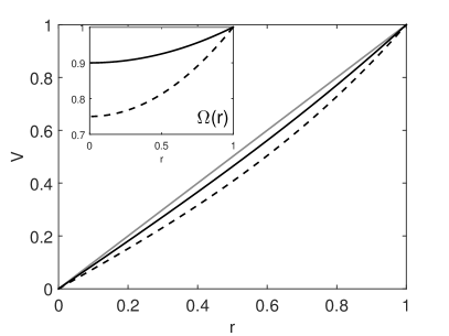
Figure 10: Radial dependence of the nondimensional total azimuthal velocity $V_{\varphi}=r+\beta U_{\beta}=(1+\beta\Omega_{\beta})r$ with $\beta=0$ (grey line), $\beta=0.1$ (black curve), $\beta=0.25$ (dashed curve). The inserted figure shows the associated angular frequencies $\Omega(r)=1+\beta\Omega_{\beta}$.

V.2 Dispersion relation of the Kelvin modes

Gunn and Aldridge Gunn and Aldridge (1990) have calculated the dispersion relation of Kelvin modes with a non-uniformly rotating fluid applying a perturbation method. In this section, we address this issue with a spectral decomposition of the solutions of equation (12) for small values of $\beta$. By using the orthogonal base formed by the solution obtained with $\beta=0$ (section II.2.2) for $m$ and $n$ given, the solutions of equation (12) are searched with the ansatz

$$(\tilde{\textbf{u}},\tilde{p})=\sum_{l=-N/2}^{N/2}a_{l}(\tilde{\textbf{u}},\tilde{p})_{0l},$$ (36)

with $a_{l}=a_{[m,n,l]}$ the amplitude of the Kelvin mode for $\beta=0$ and $(\tilde{\textbf{u}},\tilde{p})_{0l}$ taken as solutions of Eq. (13) for a given azimuthal and axial wave number $m$ and $n$. The sum is over the $N$ modes ($N$ being even) composed of the $N/2$ first retrograde modes and $N/2$ first prograde modes. They satisfy automatically the mass conservation and the boundary condition at $r=1$ and $z=\pm\Gamma^{-1}/2$. Equation (12) becomes

$$\sum_{l}a_{l}\left[i\left(\omega-\omega_{0l}\right){{\mathcal{I}}}+\beta{\mathcal{L}}_{\beta}\right](\tilde{\textbf{u}},\tilde{p})_{0l}=0$$ (37)

$\mathcal{L}_{0}(\tilde{\textbf{u}},\tilde{p})_{0l}=-\omega_{0l}(\tilde{\textbf{u}},\tilde{p})_{0l}$ and ${\mathcal{I}}$ the matrix defined by equation (59) in appendix A.1. In order to obtain a linear system coupling the coefficients, the equation is projected on the Kelvin modes $(\tilde{\textbf{u}},\tilde{p})_{0j}$ via the scalar product $\langle(\tilde{\textbf{u}},\tilde{p})_{0j},\cdot\rangle$. The resulting decomposition consists of $N$ linear equations given by

$$i\left(\omega-\omega_{0j}\right)e_{jj}a_{j}-i\beta\sum_{l}a_{l}q_{jl}=0$$ (38)

with $q_{jl}=i\langle{{(\tilde{\textbf{u}},\tilde{p})}}_{0j},{\mathcal{L}}_{\beta}{{(\tilde{\textbf{u}},\tilde{p})}}_{0{{l}}}\rangle$ and $e_{jj}=\langle(\tilde{\textbf{u}},\tilde{p})_{0j},(\tilde{\textbf{u}},\tilde{p})_{0j}\rangle$. This system can be written as a general eigenvalue problem

$$\omega\mathcal{E}\textbf{a}_{l}=\left(\mathcal{E}\mathcal{D}_{0}+\beta\mathcal{Q}\right)\textbf{a}_{l}$$ (39)

with $\mathcal{D}_{0}$ (resp. $\mathcal{E}$) the diagonal matrix of elements $\omega_{0j}$ (resp. $e_{jj}$). The elements of the matrices $\mathcal{Q}$ are given by $q_{{jl}}$. The solutions of the equation (39) are the generalized eigenmodes described by the set of eigenvectors $\textbf{a}_{l}$ and the corresponding eigenfrequencies $\omega_{l}$ indexed by $l$.

The modified background flow $\Omega_{\beta}$ given by (35) can be decomposed into a shear component (the quadratic term) and a solid body rotation (the constant term). If we only consider the constant term, the frequency detuning would be $\omega=\omega_{0}+\beta(m-\omega_{0})$ because for this simple case the matrix $\mathcal{Q}$ is diagonal and equal to $\mathcal{E}\left(-\mathcal{D}_{0}+m\mathcal{I}\right)$. Hence, the off-diagonal terms in $\mathcal{Q}$ are only due to the shear component. It is worth noting that the dispersion relation for the geostrophic mode ($k=0$) becomes

$$\omega_{l}\mathcal{E}\textbf{a}_{l}=\beta\mathcal{Q}\textbf{a}_{l}$$ (40)

because in that case $\mathcal{D}_{0}$ is a null matrix. The frequencies $\omega_{l}$ are the eigenfrequencies of $\mathcal{E}^{-1}\mathcal{Q}$ multiplied by $\beta$. Hence, the shear removes the frequency degeneracy, i.e. all the frequencies depart from $\omega_{0}=0$ and increase linearly with $\beta$.

V.3 Effect of shear on forced Kelvin modes

We now solve Eq. (39) numerically using the method described in the appendix A.2 including the benchmarking of our results against the ones obtained by a code based on the Chebyshev pseudo-spectral method Antkowiak and Brancher (2007).

We start with the frequencies of the Kelvin mode with $(m,n)=(1,1)$ and vary $\beta$ in the range $[0,0.5]$. We focus on the first five retrograde and prograde modes ($|l|<5$). The evolution of the frequencies is represented in Fig. 11 for the retrograde (a) and prograde (b) modes. For the retrograde (respectively the prograde) modes, the largest (resp. smallest) frequencies correspond to the mode with the smallest radial wave number for a given $\beta$. Initially, the frequencies increase linearly as a function of $\beta$ implying that the retrograde modes accelerate and the prograde modes decelerate. This effect can be partially explained by the Doppler effect $\omega=\omega_{0}+\beta(m-\omega_{0})$ caused by the slowdown of the solid body rotation. The factor $(m-\omega_{0})$ being positive for the considered Kelvin modes, yields the increase of the frequency (Doppler shift). An exception is the first retrograde mode with $l=1$, which is only weakly impacted by the modification of the solid body rotation because $\omega_{0}\simeq m=1$ (it is almost standing in the turntable reference frame). For increasing $\beta$ we observe a deviation of the linear detuning, which would correspond to the tangents at the origin represented by the dashed lines in Fig. 11. The departure of the retrograde and prograde modes from the linear behavior occurs approximately for $\beta>0.2$. The initial prograde mode may even become retrograde as, e.g., the prograde mode with $l=-5$ for $\beta>0.4$. For large $\beta$, the frequencies $\omega{{{}_{l}}}$ of the retrograde modes become tangent to $\beta$ (dotted line).

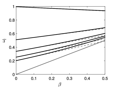
(a)

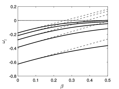
(b)

Figure 11: Evolution of the first five eigenfrequencies $\omega_{l}$ (black) of the retrograde modes with $l\in[1;5]$ (a) and prograde modes with $l\in[-5;-1]$ (b) with $m=1$ and $n=1$ as a function of the shear amplitude $\beta$. Dashed lines correspond to the tangent at the origin. The dotted line corresponds to the line, where $\omega{{{}_{l}}}=\beta$ for (a) and $\omega_{{l}}=0$ for (b).

V.4 Effect of shear on free Kelvin modes

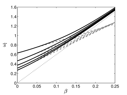
(a)

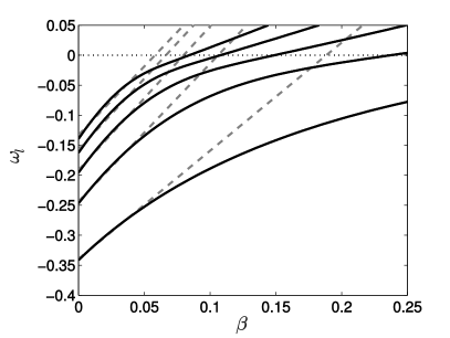
(b)

Figure 12: Dependence of the first five eigenfrequencies $\omega_{{l}}$ (solid black line) of the retrograde modes with $(m,n)=(6,2)$ (a) and the prograde modes with $(m,n)=(5,1)$ on the shear amplitude $\beta$. Dashed lines correspond to the tangent at the origin. The dotted line in (a) corresponds to the critical line, where $\omega_{{l}}=6\beta$.

We focus on the modes $(m,n)=(6,2)$ and $(5,1)$ which we assigned to the unstable Kelvin modes with the frequencies $\Omega_{2}$ and $\Omega_{3}$ observed in the experiment. We recall that the mode $(6,2)$ is retrograde whereas the mode $(5,1)$ is prograde. The dependence of the first five retrograde modes with $m=6{{,n=2}}$ and prograde modes with $m=5{{,n=1}}$ on $\beta$ is shown in Fig. 12a and b. A visible departure from the tangent at the origin occurs for $\beta{\ {\gtrsim}}0.07$ for the retrograde mode 12a, and for $\beta{{\gtrsim}}0.05$ for the prograde mode 12b. Hence, the linear detuning is only valid for small values of $\beta$. This property is important for the conditions of the parametric resonance, as we will see below. The frequencies of the retrograde modes approach $\omega_{l}=6\beta$ for large $\beta$. In the following we concentrate on the behavior of the first prograde and the first retrograde mode. Figure 13a shows the absolute value of the frequencies of the first prograde mode $(5,1,-1)$ (${{\omega_{2}}}$), the first retrograde mode $(6,2,1)$ (${{\omega_{3}}}$) and their difference $\omega_{3}-\omega_{2}$. The frequencies follow a similar behavior as the observed frequencies $\Omega 2$ and $\Omega 3$ in Fig. 6. At $\beta=0$, the difference is equal to $\omega_{3}-\omega_{2}=0.97$ and the exact resonance, i.e. $\omega_{3}-\omega_{2}=1$, occurs at $\beta=0.044$. In the range $\beta\in[0,0.2]$, the difference $\omega_{3}-\omega_{2}$ is well approximated by a polynomial expansion (grey curve in Fig. 13a)

$$\omega_{3}-\omega_{2}\simeq\delta\omega_{(0)}+\beta\delta\omega_{(1)}+\beta^{2}\delta\omega_{(2)}+\Delta$$ (41)

with $\delta\omega_{(0)}=0.97$ , $\delta\omega_{(1)}=0.172$, $\delta\omega_{(2)}=10.8$, and a residual $\Delta$ of order $|\Delta|\simeq 3\times 10^{-3}$. The quadratic term becomes significant for $\beta=\delta\omega_{(1)}/\delta\omega_{(2)}=0.017$, i.e. already before the exact resonance at $\beta=0.044$. This expansion shows that the quadratic detuning is required in the vicinity of the exact resonance, since the linear detuning underestimates the departure from the resonance even for small amplitudes of $\beta$. We point out that the exact resonant interaction at $\beta=0.044$ of the first prograde $[(m,n,l)=(5,1,-1)]$ and the first retrograde $[(m,n,l)=(6,2,1)]$ modes with the forced mode occurs well before a sequence of possible exact resonances between higher radial wave numbers. Figure 13b shows the frequencies $\omega_{3}$ (black curves) and $1+\omega_{2}$ (dashed curves) for the first four retrograde and prograde modes such that their intersection corresponds to a resonance (black circles). We see that for $\beta>0.1$, a large number of resonances occurs between modes with larger radial wave number. These resonances could trigger instabilities, which would be an efficient mechanism to transfer energy from large ($m=1$) to small scales like observed in the resonance collapse. This phenomenon suggests that the shear of the background flow could play an important role during the resonant collapse. A similar idea was proposed in Gunn and Aldridge (1990).

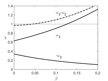
(a)

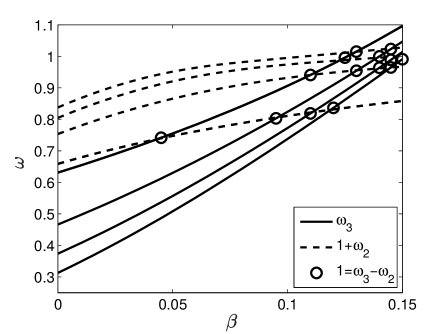
(b)

Figure 13: (a) Frequencies $\omega_{3}$ and $\omega_{2}$ of free Kelvin modes, corresponding to $(m,n,l)=(6,2,1)$ and $(5,1,-1)$, as a function of $\beta$. The dashed line represents the difference $\omega_{3}-\omega_{2}$, such that its intersection with the dotted grey line corresponds to an exact resonance. The thick grey curve (below the dashed line) corresponds to the polynomial expansion of $\omega_{3}-\omega_{2}$ given by (41). (b) The black curves show to the frequencies $\omega_{{3}}$ of the first four retrograde modes with $(m,n)=(6,2)$. The dashed lines correspond to the shifted frequencies $\omega_{{2}}+1$ of the first four prograde modes with $(m,n)=(5,1)$. The circles indicate the exact resonance between the modes, where $\omega_{3}-\omega_{2}=1$.

VI Effect of the shear on the parametric resonance of Kelvin modes

VI.1 Formulation of the parametric resonance of Kelvin modes

In this section, we study the effect of the detuning on the condition of parametric resonance. We consider a parametric instability of a single forced Kelvin mode $\gamma\textbf{u}_{0}$ of amplitude $\gamma$ and wave numbers $(m,n,l)=(1,1,1)$, via wave-interactions with two infinitesimal perturbations $(\xi\textbf{u}^{(a)},\xi\textbf{u}^{(b)})$ with $\xi\ll 1$ with the azimuthal and axial wave numbers $(m_{a},n_{a})$ and $(m_{b},n_{b})$. According to Kerswell (1999), we assume that the total velocity field u can be decomposed into

$$\textbf{u}=\gamma\textbf{u}_{0}(\textbf{r},t)+\xi\textbf{u}^{(a)}(\textbf{r},t)+\xi\textbf{u}^{(b)}(\textbf{r},t)$$ (42)

with

$$\left\{\begin{array}[]{ll}\textbf{u}_{0}&=\textbf{u}_{111}(r,z)e^{i(\varphi+t)}+c.c.\\ \\ \textbf{u}^{(a)}&=\sum\limits_{j}a_{j}(t)\textbf{u}_{m_{a}n_{a}j}(r,z)e^{im_{a}\varphi}+c.c.\\ \\ \textbf{u}^{(b)}&=\sum\limits_{l}b_{l}(t)\textbf{u}_{m_{b}n_{b}l}(r,z)e^{im_{b}\varphi}+c.c.\end{array}\right.$$ (43)

The modes $\textbf{u}^{(a)}$ and $\textbf{u}^{(b)}$ are decomposed as sums of Kelvin modes with different radial wave number indexed respectively by $j$ and $l$, and associated with the complex amplitudes $a_{j}$ and $b_{{l}}$. The velocity components $u_{mnl}(r,z)$ are given by Eq. (17), and satisfy the boundary conditions (8). For $\beta=0$, the amplitude of the modes $a_{j}$ and $b_{l}$ are associated to their eigenfrequencies $\omega_{0j}^{(a)}$ and $\omega_{0l}^{(b)}$ (see section V.2). Following the approach of Kerswell Kerswell (1999), we now consider two Kelvin modes satisfying the spatial resonance conditions so that their axial and azimuthal wave numbers fulfil the relations

$$\left\{\begin{array}[]{ll}m_{a}-m_{b}=&1\\ \\ |n_{a}-n_{b}|=&1\end{array}\right.$$ (44)

There is no restriction for the resonance in terms of radial wave numbers. An exact resonance between two modes indexed by $j$ and $l$ occurs if their frequencies satisfy the temporal resonance condition

$${{\omega_{0j}^{(a)}-\omega_{0l}^{(b)}=1}}.$$ (45)

However, the relations (44) and (45) require particular conditions in terms of a suitable aspect ratio in order to be fulfilled simultaneously for all contributing modes. In the following, we assume that the frequency condition (45) can be relaxed in order to achieve near-resonance. The azimuthal wave number and the index of the axial wave number must be integers (if $n$ is not an integer, it violates the boundary condition at the end-caps). Thus, only the condition on the frequency can be changed into a near-resonance condition by introducing the parameter

$$\Delta\omega_{0}=\frac{1}{2}\left(\omega_{0j}^{(a)}-\omega_{0l}^{(b)}-1\right).$$ (46)

We now consider the dimensionless inviscid Navier-Stokes equation expressed in the cylinder reference frame including the non-linear terms but with $\beta=0$

$$\partial_{t}\textbf{u}=-2\textbf{e}_{z}\times\textbf{u}-\nabla p+\textbf{u}\times\left(\nabla\times\textbf{u}\right).$$ (47)

Inserting ansatz (43) in (47) and projecting respectively onto the modes $\textbf{u}^{(a)}$ and $\textbf{u}^{(b)}$ we obtain two equations for the amplitudes $a_{j}$ and $b_{l}$ given by

$$\left\{\begin{array}[]{ll}\dot{a}_{j}=i\omega^{(a)}_{0j}a_{j}+c_{jl}^{(a)}\gamma b_{l}e^{it},\\ \\ \dot{b}_{l}=i\omega^{(b)}_{0l}b_{l}+c_{lj}^{(b)}\gamma^{*}a_{j}e^{-it}\end{array}\right.$$ (48)

with $c_{jl}^{(a)}$ and $c_{lj}^{(b)}$ denoting coupling terms given by Kerswell (1999)

$$\left\{\begin{array}[]{ll}c_{jl}^{(a)}=\displaystyle{\frac{1}{e_{jj}^{(a)}}{2\pi}{\Gamma}\left(\frac{\omega_{0l}^{(b)}-n_{{b}}}{\omega_{0l}^{(b)}}\right)\left\langle\textbf{u}_{0j}^{(a)}\cdot\left(\textbf{u}_{0l}^{(b)}\times\textbf{u}_{0}\right)\right\rangle},\\ \\ c_{lj}^{(b)}=\displaystyle{\frac{1}{e_{ll}^{(b)}}{2\pi}{\Gamma}\left(\frac{\omega_{0j}^{(a)}-n_{{a}}}{\omega_{0j}^{(a)}}\right)\left\langle\textbf{u}_{0l}^{(b)}{}\cdot\left(\textbf{u}_{0j}^{(a)}\times\textbf{u}_{0}{}^{*}\right)\right\rangle.}\end{array}\right.$$ (49)

where $\textbf{u}^{(a)}_{0j}$ (respectively $\textbf{u}^{(b)}_{0l}$) is the unperturbed eigenfunction given by (17) and (23) with the indices $j$ (respectively l) representing the $j$th (respectively $l$th) solution of the dispersion relation and the indizes $m$ and $n$ being supressed for the sake of clarity (they have to be fixed a priori). Furthermore, we applied the relation between velocity and vorticity for inertial waves, $\nabla\times\textbf{u}=\left(2\pi n\Gamma/\omega\right)\textbf{u}$ Kerswell (1999). The system (48) reduces to a linear system with constant coefficients via the change of variables $(a_{j},b_{l})=(\tilde{a}_{j}e^{it/2},\tilde{b}_{l}e^{-it/2})e^{i\sigma t}$ with $(\tilde{a}_{j},\tilde{b}_{l})$ two constants and $\sigma$ the eigenvalue of system (48), with $\sigma_{r}$ its real component and $\sigma_{i}$ the imaginary component. After some algebra, we obtain the solution

$$\sigma=\frac{\omega_{0j}^{(a)}+\omega_{0l}^{(b)}}{2}\pm\sqrt{(\Delta\omega_{0})^{2}-C|\gamma|^{2}}$$ (50)

with the product $C=c_{lj}^{(a)}c_{jl}^{(b)}$ given by

$$C=\displaystyle{\frac{4\left(\pi\Gamma\right)^{2}}{e_{{{jj}}}^{(a)}e_{{ll}}^{(b)}}\frac{\left(\omega^{(b)}_{0l}-n_{{b}}+2\Delta\omega_{0}\right)\left(\omega^{(b)}_{0l}-n_{{b}}\right)}{-\omega_{0l}^{(b)}\omega_{0j}^{(a)}}}\times\left|\left\langle\textbf{u}^{(a)}_{0j}\cdot\left(\textbf{u}^{(b)}_{0l}\times\textbf{u}_{0}\right)\right\rangle\right|^{2}.$$ (51)

Note that for perfectly tuned resonance the relations (49) and (51) giving the growthrate of the instability are equivalent to Eq. (5.5) and Eq. (5.6) in Kerswell (1999). If $C$ is negative, the imaginary part of $\sigma$ always vanishes and the solution remains stable. Hence, the minimum requirement for the instability is $C>0$. For an exact resonance, i.e. $\Delta\omega_{0}=0$, the coefficient $C$ is positive if the product $\omega_{0l}^{(b)}\omega_{0j}^{(a)}$ is negative, which is always fulfilled when one mode is prograde ($\omega_{0l}^{(b)}<0$) and the other one is retrograde ($\omega_{0j}^{(a)}>0$). In that case, each mode has a positive feedback on the other mode, thus enforcing the instability. The growth rate is then given by $\sigma_{i}=\pm\sqrt{|C|}|\gamma|$, i.e. the flow is unstable for all $\gamma$ in the inviscid case. Out of resonance $\Delta\omega_{0}\neq 0$, the growth rate becomes imaginary if $\Delta\omega_{0}^{2}-C|\gamma|^{2}$ becomes negative. This requires that the coefficient $C$ must be positive, so that

$$\left\{\begin{array}[]{lll}2\Delta\omega_{0}>-(\omega_{0l}^{(b)}-n_{b})&\hbox{if}&(\omega_{0l}^{(b)}-n_{b})>0\\ \\ 2\Delta\omega_{0}<-(\omega_{0l}^{(b)}-n_{b})&\hbox{if}&(\omega_{0l}^{(b)}-n_{b})<0.\end{array}\right.$$ (52)

The parametric resonance occurs if the eigenvalue $\sigma$ has a non-vanishing imaginary contribution, i.e. when the amplitude of $|\gamma|$ is larger than $\gamma_{c}=|\Delta\omega_{0}|/\sqrt{|C|}$.

We now consider the mode $a$ given by $(m_{a},k_{a},l)=(6,2,1)$ and the mode $b$ given by $(m_{b},k_{b},j)=(5,1,-1)$ where $\Delta\omega_{0}=-1.5\times 10^{-2}$. The frequencies of the modes are given by $\omega^{(a)}=\sigma_{r}^{+}+0.5$ and $\omega^{(b)}=\sigma_{r}^{-}-0.5$, while the growthrate is $-\sigma_{i}$: the mode is stable if $\sigma_{i}\geq 0$ and it is unstable otherwise.

Initially, the frequencies are given by $\omega^{(a)}=\omega_{0j}^{(a)}$ and $\omega^{(b)}=\omega_{0l}^{(b)}$ for $\gamma=0$.

The behavior of the eigenvalues $\sigma$ in dependence of the amplitude $\gamma$ of the unstable mode is shown in figure 14a and b. Below the critical amplitude $\gamma_{c}=2.3\times 10^{-3}$, the growth rate $\sigma_{i}$ vanishes and we have two solutions with frequencies such that the resonance condition $\sigma_{r}^{+}-\sigma_{r}^{-}=\omega^{(a)}-\omega^{(b)}-1$ is not equal to zero. Both frequencies converge, eventually merging at the onset of the instability at $\gamma_{c}$. Exactly at the critical amplitude, $\sigma_{r}^{+}$ and $\sigma_{r}^{-}$ collapse. Past this bifurcation we have two solutions for $\sigma_{i}$ and the solution becomes unstable with the two frequencies of the modes being locked with a difference equal to $1$, so that $\omega^{(a)}=0.645$ and $\omega^{(b)}=-0.355$. This simple model explains the basic properties of the parametric instability but does not reproduce the frequency drifting and the disappearance of the instability for large $\epsilon$, which requires the formalism introduced in section V.1.

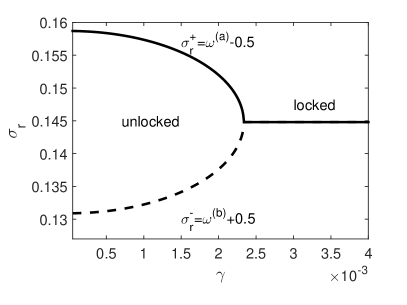
(a)

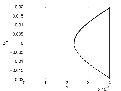
(b)

Figure 14: Frequencies $\sigma_{r}$ (a) and growth-rates $\sigma_{i}$ (b) of the eigenmodes given by the equation (50).

VI.2 Effect of the shear on the parametric instability

Now we consider the effect of shear with $\beta\neq 0$. Unlike in the previous section, the eigenmodes are no longer the original Kelvin modes because the shear couples different Kelvin modes (section V.1). The velocity decomposition (42) is now extended to

$$\textbf{u}=\gamma\textbf{u}_{0}(\textbf{r},t)+\xi\textbf{u}^{(a)}(\textbf{r},t)+\xi\textbf{u}^{(b)}(\textbf{r},t)+\beta r\Omega_{\beta}(r){\textbf{e}}_{\varphi}$$ (53)

with $\textbf{u}_{0},\textbf{u}^{(a)}$ and $\textbf{u}^{(b)}$ again given by the decomposition (43) and the last term on the right hand side corresponding to the modification of the background flow. After some algebra, the linear system coupling the $N$ amplitudes of $a_{j}$ and $b_{l}$ becomes

$$\left(\begin{array}[]{ccc}\mathcal{E}^{(a)}&&0\\ 0&&\mathcal{E}^{(b)}\end{array}\right)\frac{d\textbf{x}}{dt}=\left(\begin{array}[]{ccc}i\mathcal{N}^{(a)}&&\gamma e^{it}\mathcal{C}^{(a)}\\ \gamma^{*}e^{-it}\mathcal{C}^{(b)}&&i\mathcal{N}^{(b)}\end{array}\right)\!\textbf{x}\qquad\mbox{ with }\qquad\left\{\begin{array}[]{ll}\textbf{x}^{T}=\left(a_{1},\dots,a_{N},b_{1},\dots,b_{N}\right)\\ \\ \mathcal{N}^{(i)}=\left(\mathcal{E}\mathcal{D}_{0}+\beta\mathcal{Q}\right)^{(i)}\end{array}\right.$$ (54)

where $\mathcal{C}^{(a)}$ (respectively $\mathcal{C}^{(b)}$) is the matrix with the elements $c_{jl}^{(a)}e_{jj}^{(a)}$ (resp. $c_{lj}^{(b)}e_{{{ll}}}^{(b)}$) given by (25) and (49). When the matrices $\mathcal{C}^{(a)}$ and $\mathcal{C}^{(b)}$ are set to zeros, we recover the linear dispersion of Kelvin modes given in section V.1, and when the elements of $\mathcal{Q}$ are set to zeros, i.e. $\mathcal{N}=\mathcal{E}\mathcal{D}_{0}$, we obtain $2N$ equations describing the parametric resonance for Kelvin modes with $\beta=0$. The system (54) reduces to a linear system with constant coefficients with the change of variables

$$\textbf{x}=\left(\begin{array}[]{ccc}\mathcal{I}e^{it/2}&&0\\ 0&&\mathcal{I}e^{-it/2}\end{array}\right)\tilde{\mbox{$\textbf{x}$}}e^{i\sigma t}$$ (55)

and the eigenvalue $\sigma$ is the solution of the general eigenvalue problem

$$\sigma\left(\begin{array}[]{ccc}\mathcal{E}^{(a)}&&0\\ \\ 0&&\mathcal{E}^{(b)}\end{array}\right)\tilde{\mbox{$\textbf{x}$}}=\left(\begin{array}[]{ccc}-\frac{1}{2}\mathcal{E}^{(a)}+\mathcal{N}^{(a)}&&-i\gamma\mathcal{C}^{(a)}\\ \\ -i\gamma^{*}\mathcal{C}^{(b)}&&\frac{1}{2}\mathcal{E}^{(b)}+\mathcal{N}^{(b)}\end{array}\right)\tilde{\mbox{$\textbf{x}$}}.$$ (56)

This system is solved with the same procedure as described in section V.1.

VI.3 Application to the modes $(m,n)=(5,1)$ and $(6,2)$

Finally, we give a brief outline of an application of the theoretical framework developped in the previous section and a possibility to confirm the theory from our experimental measurements. We calculate the growthrates of free Kelvin modes in dependence of the amplitude of the modification of the background flow. Assuming that $\Omega_{1}$ is a geostrophic mode, we can linearly relate the shear amplitude $\beta$ to the precession ratio $\epsilon$, which is at least qualitatively confirmed in our measurements.

The matrices $\mathcal{E}$, $\mathcal{N}$ and $\mathcal{C}$ are calculated for prograde modes with $(m_{2},n_{2})=(5,1)$ and retrograde modes with $(m_{3},n_{3})=(6,2)$. Since we do not know the amplitude of the forced mode, we consider $\gamma$ as a free control parameter in addition to the parameter $\beta$, the amplitude of the perturbation of the solid body rotation.

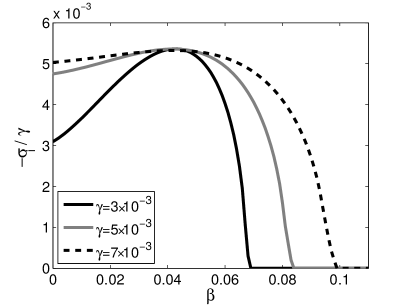
(a)

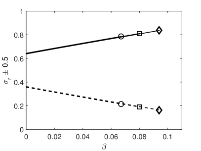
(b)

Figure 15: (a) Rescaled growth-rates $-\sigma_{i}/\gamma$ of the eigenmodes given by the system (54) as a function of $\beta$ for an amplitude of the forced mode $\gamma$ equal to $3\times 10^{-3}$ (black line), $5\times 10^{-3}$ (grey line) and $7\times 10^{-3}$ (black dashed line). (b) Corresponding frequencies $\sigma_{r}\pm\frac{1}{2}$ in the cylinder reference frame. The symbols denote the frequencies of marginal stability where $\sigma_{i}=0$, i.e. the parametric resonance switches off (circles, squares and diamonds correspond to $\gamma=3\times 10^{-3},5\times 10^{-3},7\times 10^{-3}$).

We calculate the eigenvalues $\sigma=\sigma_{r}+i\sigma_{i}$ of system (56) for three values $\gamma=[3,5,7]\times 10^{-3}$ which are above the critical value $\gamma_{\rm{c}}$ required for the onset of the instability. The parameter $\beta$ is varied in the interval $\beta\in[0,0.15]$. The results yield one unstable mode in dependence of $\beta$ and $\gamma$, which for $\beta=0$ is formed by the Kelvin modes $(6,2,1)$ and $(5,1,-1)$. The corresponding growthrates rescaled by $\gamma$ are shown in Fig.15a.

The positive growth-rate, $-\sigma_{i}$, has a maximum at the exact resonance $\beta=0.044$, (see section V.4), which increases linearly with $\gamma$ so that $\max(-\sigma_{i})={{5.3\times 10^{-3}}}\gamma$. The growthrate becomes zero when the background flow is strong enough to detune the parametric resonance. Qualitatively, the regime with resonance becomes broader (i.e. allows larger $\beta$, i.e. stronger detuning) for increasing $\gamma$. The eigenfrequencies $\sigma_{r}$ in the reference frame of the cylinder are shown in Fig. 15b. The frequencies vary almost linearly with $\beta$ and the amplitude of $\gamma$ only modifies the maximum $\beta$ at which the parametric resonance vanishes and the frequency locking ceases. The circles ($\gamma=3\times 10^{-3}$), squares ($\gamma=5\times 10^{-3}$) and diamonds ($\gamma=7\times 10^{-3}$) denote the exact locations at which unlocking of the frequencies occurs, i.e. when $\sigma_{i}$ vanishes. The marginal stability curves are shown in Fig. 16a as a function of $\gamma$ and $\beta$ (grey color for stable region and white for unstable). The unstable region describes a resonance tongue Arnolʹd (1983), which for large $\beta$ gives a threshold $\gamma_{c}\sim\beta$. This can be explained by a heuristic model when assuming that the coupling term $C$, given by Eq. (51), increases linearly with $\Delta\omega$. Fixing $\sigma_{i}=0$, the threshold $\gamma_{c}$ varies with $\Delta\omega/\sqrt{|C|}$ (Eq. 50) and we obtain $\gamma_{c}\sim\sqrt{\Delta\omega}$. On the other hand, we have shown in section V.4 that $\Delta\omega\sim\beta^{2}$ for large $\beta$, thus we obtain $\gamma_{c}\sim\beta$.

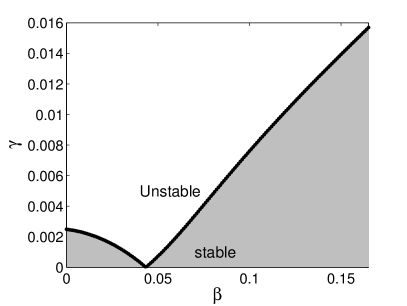
(a)

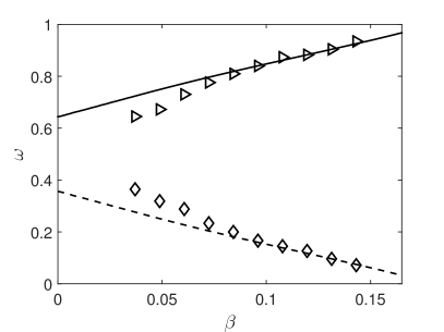
(b)

Figure 16: (a) Parameter space $(\beta,\gamma)$ with the domain of existence of the parametric instability (white region) separated by the marginal stability curve with $\sigma_{i}=0$ (black curves). (b) Frequencies corresponding to the marginal stability curve. The diamonds correspond to the experimental frequencies $\Omega_{2}$ and the triangles correspond to $\Omega_{3}$ for ${\rm{Ek}}=8.8\times 10^{-7}$ as a function of ${{\beta=}}\alpha C_{f}(\epsilon-\epsilon_{\rm{c}})$ with $C_{f}=6.23$, $\epsilon_{c}=2.5\times 10^{-2}$ and $\alpha=1.43$.

To compare numerical and experimental data, the parameters $\gamma$ and $\beta$ of the dispersion relation (56), quantifying respectively the amplitude of the forced mode and the amplitude of the shear, have to be expressed as a function of the precession ratio $\epsilon$ and the Ekman number $\rm{Ek}$. However, both parameters cannot be determined directly by the local wall-pressure measurements. To overcome this limitation we assume that the instability saturates via frequency detuning of the unstable modes (Waleffe, 1989; Lagrange et al., 2011). In our model, the saturation occurs when the shear amplitude $\beta$ reaches the marginal stability curves for a given amplitude $\gamma$. Consequently, we reduce the number of parameters to one, by only considering the parameter $\beta$ as a function of $\gamma$ all along the marginal stability curve (thick line in Fig. 16a). Figure 16b shows the curves of the theoretical frequencies $\omega_{2}$ (dashed curve) and $\omega_{3}$ (thick curve) obtained from the dispersion relation (56) as a function of $\beta$ along the marginal stability curve. In section IV.2, we showed that the experimental frequencies $\Omega_{2}$ and $\Omega_{3}$ vary with $C_{f}(\epsilon-\epsilon_{c})$ for all Ekman numbers and precession ratios $\epsilon$, with a relatively small scatter. Since the frequencies are functions of $\beta$ (from theory) and $C_{f}(\epsilon-\epsilon_{c})$ (from experiment), it is suggestive to express the shear amplitude $\beta$ as a function of $C_{f}(\epsilon-\epsilon_{c})$. The frequencies $-\Omega_{2}$ (respectively $\Omega_{3}$) are monotonically decreasing (resp. increasing) functions of $\beta(\gamma_{c})$ and/or $C_{f}(\epsilon-\epsilon_{c})$, so we conclude that the shear amplitude $\beta$ is an increasing function of $C_{f}(\epsilon-\epsilon_{c})$. Hence, the coefficient $C_{f}$ quantifies the amplitude of the shear for a given distance from the onset of instability $\epsilon-\epsilon_{c}$. We emphasize that the coefficient $C_{f}$ increases with $\rm{Ek}^{-1/4}$ (Fig. 9b), i.e. the shear increases when the Ekmann number decreases, a feature in agreement with previous observations Meunier et al. (2008); Lagrange et al. (2008). The functional form of $\beta$ finally may be deduced by assuming that the mode associated with the frequency $\Omega_{1}$ is a geostrophic mode, as suggested in section IV.4. From the dispersion relation of the geostrophic modes given by equation (40), the frequency $\Omega_{1}$ can be written as

$$\Omega_{1}=\beta/\alpha.$$ (57)

The coefficient $\alpha^{-1}$ corresponds to one of the eigenfrequencies of the matrix $\mathcal{E}^{-1}\mathcal{Q}$ (see section V.2) and is independent of $\rm{Ek}$ and $\epsilon$ by construction. Using Eq. 33, the shear amplitude $\beta$ can be written in the form

$$\beta=\alpha C_{f}(\epsilon-\epsilon_{c}).$$ (58)

Once the parameter $\alpha$ is estimated, we are able to evaluate the shear amplitude $\beta$ for any Ekman number and precession ratios so that all sets are equivalent when expressed as a function of $C_{f}(\epsilon-\epsilon_{c})$ (Fig. 8). As an example we choose the frequencies from the set of measurements at the smallest Ekman number examined within the present study (${\rm{Ek}}=8.8\times 10^{-7}$) for which we have $\epsilon_{c}=2.5\times 10^{-2}$ and $C_{f}=6.23$. The coefficient $\alpha$ is determined empirically so that the distance between experimental and numerical data is minimized. The results are shown in Fig. 16b, with $\Omega_{2}$ (diamonds) and $\Omega_{3}$ (triangles) plotted as a function $\beta$ given by (58) with $\alpha=1.43$. We observe a good agreement, even if close to the threshold the experimental frequencies differ slightly from the theoretical solutions (difference of $12\%$).

Of course, this application is based on a simple hypothesis and the model essentially relies only on two parameters. Whereas the frequency of the (hypothetic) geostrophic mode (the inverse of the eigenvalue $\alpha^{-1}$) can be computed from experimental data, it remains impossible to determine the amplitude $\gamma$ of the forced mode from our pressure measurements without elaborate measurements of the flow (PIV, Doppler probes), which could confirm our scenario.

VII Conclusion

In the present study, we have investigated experimentally and theoretically the stability of a Kelvin mode driven by precession. The instability is detected experimentally above a critical precession ratio via the appearance of peaks in the temporal power spectrum of pressure fluctuations measured at the end-walls of a precessing cylinder. All frequencies satisfy resonance conditions so that the sum or the difference of the frequencies is equal to the frequency of the forced Kelvin mode. Two sets have been identified: a triad with the frequencies $(\Omega_{\rm{c}},\Omega_{2},\Omega_{3})$ and a second set consisting of four modes $(\Omega_{\rm{c}},\Omega_{1},\Omega_{4},\Omega_{5})$. All frequencies vary with the precession ratio, while they continue to fulfil the temporal resonance condition with the forced mode. The frequency variations are significant, and cannot be explained by a viscous detuning, since the observed detuning increases when the Ekman number decreases. Similar to observations by Lin et al. (2014), each set of frequency disappears for larger precession ratio.

The first set corresponds to two free Kelvin modes characterized by $(\omega_{2},m_{2},n_{2},l_{2})=(-0.34,5,1,-1)$ and $(\omega_{3},m_{3},n_{3},l_{3})=(0.64,6,2,1)$ which result from a parametric instability of the forced mode. Comparable free Kelvin modes were found in different experiments and simulations. These modes constitute the most unstable modes in the precessing system with aspect ratio $\Gamma=R/H=0.5$, which is close to the exact $(m=1,n=1,l=1)$ resonance at $\Gamma=0.502559$ and there are nearly no doubts about this interpretation. The behavior may be different for another aspect ratio, where other free Kelvin modes emerge Giesecke et al. (2015), and where the forced mode is no longer resonant, which would result in a weaker amplitude and a different location in the stability diagram shown in Figure 16a.

We developed a consistent framework to explain the behavior of the frequencies $\Omega_{2}$ and $\Omega_{3}$, and we showed that the parametric resonance is able to lock the frequencies to maintain the resonant condition, despite the detuning due to background shear flow. However, the instability is suppressed when the amplitude of the forced mode is not sufficiently large for allowing the frequency locking. We have investigated theoretically the modification of the dispersion relation due to a non-uniformly rotating background flow. Our numerical results are in good agreement with the experimental observations: the frequency of a retrograde Kelvin mode (resp. prograde Kelvin mode) increases (resp. decreases) with the coefficient $\beta$ that parameterizes the slowdown of the background flow. We show that a slight modification of the background solid body rotation ($\beta=0.044$) is sufficient to trigger an exact resonance between the Kelvin modes. Furthermore, we have studied the effect of the detuning on the condition of parametric resonance. The frequency difference $\omega_{3}-\omega_{2}$ increases quadratically with $\beta$ and a small perturbation of the solid body rotation ($\beta\simeq 0.15$) is sufficient to unlock the frequencies so that the parametric resonance is suppressed. This feature explains the disappearance of the frequencies $\Omega_{2}$ and $\Omega_{3}$, above a critical precession ratio. At the critical point, the amplitude of the forced mode is no longer strong enough to lock the frequencies of the unstable Kelvin modes.

The identification of the modes of the second set and the nature of this instability are more speculative. At the threshold of appearance, the frequency $\Omega_{1}$ is close to zero and the frequencies $\Omega_{4}$ and $\Omega_{5}$ are close to $\Omega_{\rm{c}}=1$. This frequency set always appears at a lower critical precession ratio than required for the triadic resonances discussed above. With almost certainty we can rule out the possibility that these modes form a resonant triad and we suggest that $\Omega_{4}$ and $\Omega_{5}$ correspond to Kelvin modes resulting from the interaction of the directly forced mode and a geostrophic mode $\Omega_{1}$. In that case, the non-vanishing frequency of the geostrophic mode results from a background shear flow that removes the frequency degeneracy at $\omega_{0}=0$ in case of the background flow being an unperturbed solid body rotation. Following this hypothesis, the second set could be an experimental hint of the instability involving a geostrophic mode, predicted numerically in Kerswell (1999).

The ad-hoc parameterization of the shear amplitude $\beta$ as a function of the precession ratio $\epsilon$ is based on the hypothesis that the mode associated with the frequency $\Omega_{1}$ is a geostrophic mode. From the dispersion relation, we know that the frequency of the geostrophic mode increases linearly with $\beta$. Assuming $\Omega_{1}\propto\beta$ , we observe a good agreement between numerical prediction and the experimental results. However, without experimental confirmation of the spatial structure of the instability, the presence of a geostrophic mode remains speculative, although we find similarities between our observations and the frequency variation of the instability of a geostrophic mode described by Kerswell Kerswell (1999).

Our experimental and theoretical results point out that the saturation mechanism of the instability of a Kelvin mode is related to a modification of the background flow, which changes the dispersion relation of the Kelvin modes. The conditions of resonance are particularly sensitive to the amplitude of the background flow: a slight modification can tune or detune a resonance. Moreover, our calculations suggest that a sequence of small scale unstable modes could emerge after the disappearance of the first resonant triad. We did not detect these modes in the pressure measurements, since the power spectrum becomes flat for moderate precession ratio (see also Lin et al. (2014)). This regime is not yet turbulent Herault et al. (2015), although the flow cannot be described by a superimposition of free Kelvin modes. The nature of this regime remains enigmatic, and further numerical and experimental studies are required to characterize the features of this non-linear regime. At current stage, we presume that the instability of small scale modes may be inhibited by the viscous dissipation.

The development of the azimuthal shear is of relevance for the large precession dynamo experiment currently under construction at HZDR, where a precession-driven flow of liquid sodium is expected to generate a magnetic field Stefani et al. (2015). Simulations have shown that the modification of the azimuthal shear profile is accompanied by further instabilities, which are of great importance for the dynamo process Giesecke et al. (2018). A deeper understanding of these processes and especially a robust detection of the azimuthal flow profile in an opaque medium like a liquid metal are therefore of great importance for this experiment. The kind of “spectroscopy” of Kelvin modes as developed for this study, could be applied using the measured detuning of the parametric resonance as starting point to deduce a model of the radial profile of the azimuthal shear, which, of course will require a more sophisticated approach than the simple (quadratic) form for the rotation law, as assumed in Eq. (35).

So far the ultimate confirmation of the emergence of a geostrophic mode by directly resolving the flow structure is lacking and other possibilities for explaining our observations might be possible. For example, an altenative explanation may interpretate the frequency $\Omega_{1}$ as a ‘beat’ frequency indicative of a near-commensurate quasi-periodic response, which, however, would require different assumptions, e.g., about the origin of this near-commensurate quasi-periodic frequency. At this stage, we are not able to give a final answer to this question so that – although the scenario connected with a geostrophic mode is quite plausible – the presence and the origin of the modes $\Omega_{1},\Omega_{4},$ and $\Omega_{5}$ must remain an unsolved issue.

Appendix A Operators and solutions

A.1 Linear operators

The operators used in equation (12) read as follows

$${\mathcal{I}}=\left(\begin{array}[]{ccccccc}1&&0&&0&&0\\ \\ \vphantom{\displaystyle\frac{1}{r}}0&&1&&0&&0\\ \\ 0&&0&&1&&0\\ \\ \vphantom{\displaystyle\frac{1}{r}}0&&0&&0&&0\\ \end{array}\right)$$ (59)

$${\mathcal{L}}_{0}=\left(\begin{array}[]{ccccccc}0&&-2&&0&&\partial_{r}\\ \\ 2&&0&&0&&\displaystyle i\frac{m}{r}\\ \\ 0&&0&&0&&ik\\ \\ \displaystyle\frac{1}{r}+\partial_{r}&&\displaystyle i\frac{m}{r}&&ik&&0\\ \end{array}\right)$$ (60)

$${\mathcal{L}}_{\beta}=\left(\begin{array}[]{ccccccc}im\Omega&&-2\Omega&&0&&0\\ \\ \zeta&&im\Omega&&0&&0\\ \\ 0&&0&&im\Omega&&0\\ \\ 0&&0&&0&&0\\ \end{array}\right).$$ (61)

A.2 Numerical convergence

Equation (39) is solved via a MATLAB code. The number of involved Kelvin modes is fixed to $N=100$, i.e the first $50$ prograde and retrograde modes. We have checked the convergence by also using $N=200$. The roots of the dispersion relations (14) and (15) are solved with a residual smaller than $10^{-10}$. The scalar products $m_{jl}$ and $e_{ll}$ are calculated via a Gauss-Legendre quadrature rule, which is based on a collocation method using the Legendre polynomials as weighting functions. We used $10^{3}$ collocation points for the integration of the Bessel functions, which corresponds to $20$ points per lobe for the Kelvin modes with $l=\pm 50$. The generalized eigenvalue problem (39) is solved by using the routine EIG, which calculates the eigenvalues $\omega_{l}$ and eigenvectors $\textbf{a}_{l}$. We have checked that the residual for the first Kelvin modes, i.e $|{l}|<5$, is smaller than $10^{-10}$. Another way to verify the convergence is to validate that the imaginary part of $\omega_{l}$ is zero without dissipation (the mode remains stable).

We have verified our code by comparing our result with a code developed by Antkowiak and Brancher Antkowiak and Brancher (2007) based on the Chebyshev pseudo-spectral method Weideman and Reddy (2000). Unlike our code, the Chebyshev code respects no-slip boundary conditions. We have used a sufficient number of collocation points (typically $50$) to converge the results without resolving the boundary layer in order to mimic a free-slip condition. We fix a small Ekman number (${\rm{Ek}}<10^{-3}$) in order to neglect the viscous dissipation in the bulk flow. The difference between the eigenfrequency of our method and the Chebyshev code for $m=1$, $n=1$ and $l=(1,2,3)$, with $\omega_{0l}=(0.99,0.51,0.34)$, is shown in Fig.17. We have checked that the relative difference is small, with values of order $10^{-4}$.

We point out that our code allows to follow continuously all Kelvin modes by varying $\beta$, whereas spurious modes arise in the Chebyshev code when the resolution is increased.

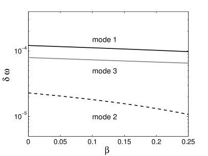
Figure 17: Difference between the eigenfrequencies calculated by a Chebyshev code and our code. The differences are calculated with the three first retro-grade modes with $m=1$ and $n=1$.

References

- Thomson (1880) W. Thomson, “Vibrations of a columnar vortex,” Philos. Mag. 10, 152–165 (1880).
- McEwan (1970) A. D. McEwan, “Inertial oscillations in a rotating fluid cylinder,” J. Fluids Mech. 40, 603–640 (1970).
- Le Bars et al. (2015) M. Le Bars, D. Cébron, and P. Le Gal, “Flows Driven by Libration, Precession, and Tides,” Annu. Rev. Fluid Mech. 47, 163–193 (2015).
- Fabre et al. (2006) David Fabre, Denis Sipp, and Laurent Jacquin, “Kelvin waves and the singular modes of the lamb–oseen vortex,” J. Fluid Mech. 551, 235–274 (2006).
- Kerswell (2002) R. R. Kerswell, “Elliptical instability,” Annu. Rev. Fluid Mech. 34, 83–113 (2002).
- Kerswell (1999) R. R. Kerswell, “Secondary instabilities in rapidly rotating fluids: inertial wave breakdown,” J. Fluids Mech. 382, 283–306 (1999).
- Giesecke et al. (2018) A. Giesecke, T. Vogt, T. Gundrum, and F. Stefani, “Nonlinear large scale flow in a precessing cylinder and its ability to drive dynamo action,” Phys. Rev. Lett. 120, 024502 (2018).
- Waleffe (1989) F. Waleffe, The 3D instability of a strained vortex and its relation to turbulence, Ph.D. thesis, Massachusetts Institute of Technology (1989).
- Greenspan (1969) H. P. Greenspan, “On the non-linear interaction of inertial modes,” J. Fluid Mech. 36, 257–264 (1969).
- Le Reun et al. (2017) T. Le Reun, B. Favier, A. J. Barker, and M. Le Bars, “Inertial wave turbulence driven by elliptical instability,” Phys. Rev. Lett. 119, 034502 (2017).
- Manasseh (1992) R. Manasseh, “Breakdown regimes of inertia waves in a precessing cylinder,” J. Fluids Mech. 243, 261–296 (1992).
- Kobine (1995) J. J. Kobine, “Inertial wave dynamics in a rotating and precessing cylinder,” J. Fluids Mech. 303, 233–252 (1995).
- Meunier et al. (2008) P. Meunier, C. Eloy, R. Lagrange, and F. Nadal, “A rotating fluid cylinder subject to weak precession,” J. Fluids Mech. 599, 405–440 (2008).
- Liao and Zhang (2012) X. Liao and K. Zhang, “On flow in weakly precessing cylinders: the general asymptotic solution,” J. Fluids Mech. 709, 610–621 (2012).
- Gans (1970) R. F. Gans, “On the precession of a resonant cylinder,” J. Fluids Mech. 41, 865–872 (1970).
- Kobine (1996) J. J. Kobine, “Azimuthal flow associated with inertial wave resonance in a precessing cylinder,” J. Fluids Mech. 319, 387–406 (1996).
- Lagrange et al. (2008) R. Lagrange, C. Eloy, F. Nadal, and P. Meunier, “Instability of a fluid inside a precessing cylinder,” Phys. Fluids 20, 081701 (2008).
- Lin et al. (2014) Y. Lin, J. Noir, and A. Jackson, “Experimental study of fluid flows in a precessing cylindrical annulus,” Phys. Fluids 26, 046604 (2014).
- Albrecht et al. (2015) T. Albrecht, H. M. Blackburn, J. M. Lopez, R. Manasseh, and P. Meunier, “Triadic resonances in precessing rapidly rotating cylinder flows,” J. Fluids Mech. 778, R1 (2015).
- Herault et al. (2015) J. Herault, T. Gundrum, A. Giesecke, and F. Stefani, “Subcritical transition to turbulence of a precessing flow in a cylindrical vessel,” Phys. Fluids 27, 124102 (2015).
- Giesecke et al. (2015) A. Giesecke, T. Albrecht, T. Gundrum, J. Herault, and F. Stefani, “Triadic resonances in nonlinear simulations of a fluid flow in a precessing cylinder,” New J. Phys. 17, 113044 (2015).
- Albrecht et al. (2018) T. Albrecht, H. M. Blackburn, J. M. Lopez, R. Manasseh, and P. Meunier, “On triadic resonance as an instability mechanism in precessing cylinder flow,” J. Fluids Mech. 841, R3 (2018).
- Lagrange et al. (2011) R. Lagrange, P. Meunier, F. Nadal, and C. Eloy, “Precessional instability of a fluid cylinder,” J. Fluids Mech. 666, 104–145 (2011).
- Mouhali et al. (2012) W. Mouhali, T. Lehner, J. Léorat, and R. Vitry, “Evidence for a cyclonic regime in a precessing cylindrical container,” Exp. Fluids 53, 1693–1700 (2012).
- Hof et al. (2006) B. Hof, J. Westerweel, T. M. Schneider, and B. Eckhardt, “Finite lifetime of turbulence in shear flows,” Nature 443, 59–62 (2006).
- Lopez and Marques (2016) J. M. Lopez and F. Marques, “Nonlinear and detuning effects of the nutation angle in precessionally forced rotating cylinder flow,” Phys. Rev. Fluids 1, 023602 (2016).
- Greenspan (1968) H. P. Greenspan, The Theory of Rotating Fluids, Cambridge Monographs on Mechanics (Cambridge University Press, 1968).
- Manasseh (1994) R. Manasseh, “Distortions of inertia waves in a rotating fluid cylinder forced near its fundamental mode resonance,” J. Fluids Mech. 265, 345–370 (1994).
- Kerswell and Barenghi (1995) R. R. Kerswell and C. F. Barenghi, “On the viscous decay rates of inertial waves in a rotating circular cylinder,” J. Fluid Mech. 285, 203–214 (1995).
- Marques and Lopez (2015) F. Marques and J. M. Lopez, “Precession of a rapidly rotating cylinder flow: traverse through resonance,” J. Fluids Mech. 782, 63–98 (2015).
- Lopez and Marques (2018) J. M. Lopez and F. Marques, “Rapidly rotating precessing cylinder flows: forced triadic resonances,” J. Fluid Mech. 839, 239–270 (2018).
- Chandrasekhar (1961) S. Chandrasekhar, Hydrodynamic and Hydromagnetic Stability, Dover Books on Physics Series (Dover Publications, 1961).
- Gunn and Aldridge (1990) J. S. Gunn and K. D. Aldridge, “Inertial wave eigenfrequencies for a nonuniformly rotating fluid,” Phys. Fluids 2, 2055–2060 (1990).
- Antkowiak and Brancher (2007) A. Antkowiak and P. Brancher, “On vortex rings around vortices: an optimal mechanism,” J. Fluid Mech. 578, 295–304 (2007).
- Arnolʹd (1983) V. I. Arnolʹd, Geometrical methods in the theory of ordinary differential equations (Springer, 1983).
- Stefani et al. (2015) F. Stefani, T. Albrecht, G. Gerbeth, A. Giesecke, T. Gundrum, J. Herault, C. Nore, and C. Steglich, “Towards a precession driven dynamo experiment,” Magnetohydrodynamics 51, 275–284 (2015).
- Weideman and Reddy (2000) J. A. Weideman and S. C. Reddy, “A matlab differentiation matrix suite,” ACM Transactions on Mathematical Software (TOMS) 26, 465–519 (2000).