Pure Exploration in Infinitely-Armed Bandit Models with Fixed-Confidence

Abstract

We consider the problem of near-optimal arm identification in the fixed confidence setting of the infinitely armed bandit problem when nothing is known about the arm reservoir distribution. We (1) introduce a PAC-like framework within which to derive and cast results; (2) derive a sample complexity lower bound for near-optimal arm identification; (3) propose an algorithm that identifies a nearly-optimal arm with high probability and derive an upper bound on its sample complexity which is within a log factor of our lower bound; and (4) discuss whether our $\log^{2}\frac{1}{\delta}$ dependence is inescapable for “two-phase” (select arms first, identify the best later) algorithms in the infinite setting. This work permits the application of bandit models to a broader class of problems where fewer assumptions hold.

Keywords: Infinitely-Armed Bandit Models, Pure Exploration

1 Introduction

We present an extension of the stochastic multi-armed bandit (MAB) model, which is applied to many problems in computer science and beyond. In a bandit model, an agent is confronted with a set of arms that are unknown probability distributions. At each round $t$, the agent chooses an arm to play, based on past observation, after which a reward drawn from the arm’s distribution is observed. This sequential sampling strategy (“bandit algorithm”) is adjusted to optimize some utility measure. Two measures are typical: cumulative regret minimization and pure exploration. For regret minimization, one attempts minimize regret, the difference between the expected cumulative rewards of an optimal strategy and the employed strategy. In the pure-exploration framework, one seeks the arm with largest mean irrespective of the observed rewards. Two dual settings have been studied: the fixed-budget setting, wherein one can use only a given number of arm-pulls, and the fixed-confidence setting, wherein one attempts to achieve a utility target with minimal arm-pulls.

While the literature mainly considers bandit models with a known, finite number of arms, for many applications the number of arms may be very large and even infinite. In these cases, one can often settle for an arm which is “near” the best in some sense, as such an arm can be identified at significantly less cost. One such application is machine learning: given a large pool of possible classifiers (arms), one wants to find the one with minimal risk (mean reward) by sequentially choosing a classifier, training it and measuring its empirical test error (reward). In text, image, and video classification, one often encounters effectively infinite sets of classifiers which are prohibitively expensive to assess individually. Addressing such cases with bandit models is particularly useful when used within ensemble algorithms such as AdaBoost (Freund and Schapire, 1996), and some variations on this idea have already been explored (Appel et al., 2013; Busa-Fekete and Kégl, 2010; Dubout and Fleuret, 2014; Escudero et al., 2001), though the task of efficiently identifying a near-optimal classifier is at present unsolved. We here approach such problems from a theoretical standpoint.

Two distinct lines of work address a potentially infinite set of arms. Let $\mathcal{W}$ be a (potentially uncountable) set of arms and assume that there exists $\mu:\mathcal{W}\rightarrow\mathbb{R}$, a mean-reward mapping such that when some arm $w$ is selected, one observes an independent draw of a random variable with mean $\mu(w)$. One line of research (Kleinberg et al., 2008; Bubeck et al., 2011b; Grill et al., 2015) assumes that $\mathcal{W}$ is some metric space, and that $\mu$ has some regularity property with respect to the metric (for example it is locally-Lipschitz). Both regret minimization and fixed-budget pure-exploration problems have been studied in this setting. Another line of research, starting with the work of Berry et al. (1997) assumes no particular structure on $\mathcal{W}$ and no regularity for $\mu$. Rather, there is some reservoir distribution on the arms’ means (the set $\mu(\mathcal{W})$ with our notation) such that at each round the learner can decide to query a new arm, whose mean is drawn from the reservoir, and sample it, or to sample an arm that was previously queried. While regret minimization was studied by several authors (Wang et al., 2009; Bonald and Proutière, 2013; David and Shimkin, 2014), the recent work of Carpentier and Valko (2015) is the first to study the pure-exploration problem in the fixed-budget setting.

We present a novel theoretical framework for the fixed-confidence pure-exploration problem in an infinite bandit model with a reservoir distribution. The reservoir setting seems well-suited for machine learning, since it is not clear whether the test error of a parametric classifier is smooth with respect to its parameters. Typically, an assumption is made on the form of the tail of the reservoir which allows estimation of the probability that an independently-drawn arm will be “good;” that is, close to the best possible arm. However, for problems such as that mentioned above such an assumption does not seem warranted. Instead, we employ a parameter, $\alpha$, indicating the probability of independently drawing a “good” arm. When a tail assumption can be made, $\alpha$ can be computed from this assumption. Otherwise, it can be chosen based on the user’s needs. Note that the problem of identifying a “top-$\alpha$” arm in the infinite case corresponds to the finite case problem of finding one of the top $m$ arms from a set of $n$ arms, for $n>m$, with $\alpha=m/n$. The first of two PAC-like frameworks we introduce, the $(\alpha,\delta)$ framework, aims to identify an arm in the top-$\alpha$ tail of the reservoir with probability at least $1-\delta$, using as few samples as possible.

We now motivate our second framework. When no assumptions can be made on the reservoir, one may encounter reservoirs with large probability masses close to the boundary of the top-$\alpha$ tail. Indeed, the distribution of weighted classifier accuracies in later rounds of AdaBoost has this property, as the weights are chosen to drive all classifiers toward random performance. This is a problem for any framework defined purely in terms of $\alpha$, because such masses make us likely to observe arms which are not in the top-$\alpha$ tail but which are hard to distinguish from top-$\alpha$ arms. However, in practice their similarity to top-$\alpha$ arms makes them reasonable arms to select. For this reason we add an $\epsilon$ relaxation, which limits the effort spent on arms near the top-$\alpha$ tail while adding directly to the simple regret a user may observe. Formally, our $(\alpha,\epsilon,\delta)$ framework seeks an arm within $\epsilon$ of the top-$\alpha$ fraction of the arms with probability at least $1-\delta$, using as few samples from the arms as possible.

Although $\alpha$ and $\epsilon$ both serve to relax the goal of finding an arm with maximum mean, they have distinct purposes and are both useful. One might wonder, if the inverse CDF $G^{-1}$ for the arm reservoir was available (at least at the tail), why one would not simply compute $\epsilon^{\prime}=\epsilon+G^{-1}(1-\alpha)$ and use the established $(\epsilon,\delta)$ framework. Indeed, $\alpha$ is important precisely when the form of the reservoir tail is unknown. The user of an algorithm will wish to limit the effort spent in finding an optimal arm, and with no assumptions on the reservoir $\epsilon$ alone is insufficient to limit an algorithm’s sample complexity. Just as there might be large probability close to the $\alpha$ boundary, it may be that there is virtually no probability within $\epsilon$ of the top arm. The user applies $\alpha$ to (effectively) specify how hard to work to estimate the reservoir tail, and $\epsilon$ to specify how hard to work to differentiate between individual arms.

Our approach differs from the typical reservoir setting in that it does not require any regularity assumption on the tail of the reservoir distribution, although it can take advantage of one when available. Within this framework, we prove a lower bound on the expected number of arm pulls necessary to achieve $(\alpha,\delta)$ or $(\alpha,\epsilon,\delta)$ performance by generalizing the information-theoretic tools introduced by Kaufmann et al. (2016) in the finite MAB setting. We also study a simple algorithmic solution to the problem based on the KL-LUCB algorithm of Kaufmann and Kalyanakrishnan (2013), an algorithm for $\epsilon$-best arm identification in bandit models with a finite number of arms, and we compare its performance to our derived lower bound theoretically. Our algorithm is an $(\alpha,\epsilon,\delta)$ algorithm, but we show how to achieve $(\alpha,\delta)$ performance when assumptions can be made on the tail of the reservoir.

We introduce the $(\alpha,\delta)$ and $(\alpha,\epsilon,\delta)$ frameworks and relate them to existing literature in Section 2. Section 3 proves our sample complexity lower bounds. In Section 4, we present and analyze the $(\alpha,\epsilon)$-KL-LUCB algorithm for one-dimensional exponential family reward distributions. A comparison between our upper and lower bounds can be found in Section 4.4. We defer most proofs to the appendix, along with some numerical experiments.

2 Pure Exploration with Fixed Confidence

Here we formalize our frameworks and connect them to the existing literature.

2.1 Setup, Assumptions, and Notation

Let $(\mathcal{W},\mathcal{F}_{\mathcal{W}},M)$ be a probability space over arms with measure $M$, where each arm $w\in\mathcal{W}$ is some abstract object (e.g. a classifier), and let $(\Theta,\mathcal{F}_{\Theta})$ be a measurable space over expected rewards, where $\Theta\subseteq\mathbb{R}$ is a continuous interval and $\mathcal{F}_{\Theta}$ is the Borel $\sigma$-algebra over $\Theta$ (i.e. the smallest $\sigma$-algebra containing all sub-intervals of $\Theta$). Also let $P_{\Theta}=\mathchoice{\left\{p_{\theta},\theta\in\Theta\right\}}{\{p_{\theta},\theta\in\Theta\}}{\{p_{\theta},\theta\in\Theta\}}{\{p_{\theta},\theta\in\Theta\}}$ be a parametric set of probability distributions such that each distribution is continuously parameterized by its mean. To ease the notation, we shall assume $\mathds{E}_{X\sim p_{\theta}}[X]=\theta$. One can think of $P_{\Theta}$ as a one-parameter exponential family (e.g. the family of Bernoulli, Gaussian with fixed and known variance, Poisson or Exponential distributions with means in some interval or other subset of $\mathbb{R}$), however we do not limit ourselves to such well-behaved reward distributions. We defer our further assumptions on $P_{\Theta}$ to Section 3.1. We will denote by $f_{\theta}$ the density of the element in $P_{\Theta}$ with mean $\theta$.

An infinite bandit model is characterized by a probability measure $M$ over $(\mathcal{W},\mathcal{F}_{\mathcal{W}})$ together with a measurable mapping $\mu:\mathcal{W}\rightarrow\Theta$ assigning a mean $\theta$ (and therefore a reward distribution $p_{\theta}$) to each arm. The role of the measure $M$ is to define the top-$\alpha$ fraction of arms, as we will show in Eq. 2; it can be used by the algorithm to sample arms. At each time step $t$, a user selects an arm $W_{t}\in\mathcal{W}$, based on past observation. He can either query a new arm in $\mathcal{W}$ (which may be sampled $W_{t}\sim M$, or selected adaptively) or select an arm that has been queried in previous rounds. In any case, when arm $W_{t}$ is drawn, an independent sample $Z_{t}\sim p_{\mu(W_{t})}$ is observed.

For example, when boosting decision stumps (binary classifiers which test a single feature against a threshold), the set of arms $\mathcal{W}$ consists of all possible decision stumps for the corpus, and the expected reward for each arm is its expected accuracy over the sample space of all possible classification examples. An algorithm may choose to draw the arms at random according to the probability measure $M$; this is commonly done by, in effect, placing uniform probability mass over the thresholds placed halfway between the distinct values seen in the training data and placing zero mass over the remaining thresholds. We are particularly interested in the case when the number of arms in the support for $M$ is so large as to be effectively infinite, at least with respect to the available computational resources.

We denote by $\mathbb{P}_{\mu}^{M}$ and $\mathds{E}_{\mu}^{M}$ the probability and expectation under an infinite bandit model with arm probability measure $M$ and mean function $\mu$. The history of the bandit game up to time $t$ is $H_{t}=((W_{1},Z_{1}),\dots,(W_{t},Z_{t})).$ By our assumption, the arm selected at round $t$ only depends on $H_{t-1}$ and $U_{t}$, which is uniform on $[0,1]$ and independent of $H_{t-1}$ (used to sample from $M$ if needed). In particular, the conditional density of $W_{t}$ given $H_{t-1}$, denoted by $\mathbb{P}_{\mu}^{M}\left(W_{t}|H_{t-1}\right)$, is independent of the mean mapping $\mu$. Note that this property is satisfied as well if, when querying a new arm, $W_{t}$ can be chosen arbitrarily in $\mathcal{W}$ (depending on $H_{t-1}$), and not necessarily at random from $M$. Under these assumptions, one can compute the likelihood of $H_{T}$:

$$\ell\left(H_{T};\mu,M\right)=\prod_{t=1}^{T}f_{\mu(W_{t})}(Z_{t})\mathbb{P}_{\mu}^{M}\left(W_{t}|H_{t-1}\right).$$ (1)

Note that the arms $W_{t}$ are not latent objects: they are assumed to be observed, but not their means $\mu(W_{t})$. For instance, in our text classification example we know the classifier we are testing but not its true classification accuracy. Treating arms as observed in this way simplifies the likelihood by making the choice of new arms to query independent of their mean mappings. This is key to our approach to dealing with reservoirs about which nothing is known; we can avoid integrating over such reservoirs and so do not require the reservoir to be smooth. For details, see Appendix A.1.

2.2 Objective and Generic Algorithm

Reservoir distribution.

The probability space over arms $(\mathcal{W},\mathcal{F}_{\mathcal{W}},M)$ and the mapping $\mu$ is used to form a pushforward measure over expected rewards $M_{\Theta}(\mathcal{E}):=(\mu_{*}(M))(\mathcal{E})=M(\mu^{-1}(\mathcal{E})),\text{ for }\mathcal{E}\in\mathcal{F}_{\Theta},$ inducing the probability space $(\Theta,\mathcal{F}_{\Theta},M_{\Theta})$ over expected rewards. We define our reservoir distribution CDF $G(\tau)=M_{\Theta}(\mathchoice{\left\{\theta\leq\tau\right\}}{\{\theta\leq\tau\}}{\{\theta\leq\tau\}}{\{\theta\leq\tau\}})$ whose density $g$ is its Radon-Nikodym derivative with respect to $M$. For convenience, we also define the “inverse” CDF $G^{-1}(p):=\inf\mathchoice{\left\{\theta:G(\theta)\geq p\right\}}{\{\theta:G(\theta)\geq p\}}{\{\theta:G(\theta)\geq p\}}{\{\theta:G(\theta)\geq p\}}.$ We assume that $G$ has bounded support and let $\mu^{*}$ be the largest possible mean under the reservoir distribution, $\mu^{*}:=G^{-1}(1)=\inf\mathchoice{\left\{\theta:G(\theta)=1\right\}}{\{\theta:G(\theta)=1\}}{\{\theta:G(\theta)=1\}}{\{\theta:G(\theta)=1\}}.$

In the general setup introduced above, the reservoir may or may not be useful to query new arms, but it is needed to define the notion of top-$\alpha$ fraction.

Finding an arm in the top-$\alpha$ fraction.

In our setting, for some fixed $\alpha\in]0,1[$ and some $\epsilon\geq 0$, the goal is to identify an arm that belongs to the set

$$\mathcal{G}_{M,\mu}^{\alpha,\epsilon}:=\mathchoice{\left\{w\in\mathcal{W}:\mu(w)\geq G^{-1}(1-\alpha)-\epsilon\right\}}{\{w\in\mathcal{W}:\mu(w)\geq G^{-1}(1-\alpha)-\epsilon\}}{\{w\in\mathcal{W}:\mu(w)\geq G^{-1}(1-\alpha)-\epsilon\}}{\{w\in\mathcal{W}:\mu(w)\geq G^{-1}(1-\alpha)-\epsilon\}}$$ (2)

of arms whose expected mean rewards is high, in the sense that their mean is within $\epsilon$ of the quantile of order $1-\alpha$ of the reservoir distribution. For notational convenience, when we set $\epsilon$ to zero we write $\mathcal{G}_{M,\mu}^{\alpha}:=\mathcal{G}_{M,\mu}^{\alpha,0}$.

0:  Arm set $\mathcal{W}$, target $\alpha,\epsilon,\delta$

0:  Some arm $\hat{s}$

  for $t\leftarrow 1,2,\dots$ do

     (choose one of:)

1. Pull arm: Choose $W_{t}\sim\mathbb{P}_{\mu}^{M}\left(W_{t}|H_{t-1}\right)$ and observe reward $Z_{t}\sim p_{\mu(W_{t})}$

2. Stop: Choose $\hat{s}\leftarrow W_{s}$ for some $s<t$,

   return $\hat{s}$

  end for

Algorithm 1 Generic algorithm.

Generic algorithm

An algorithm is made of a sampling rule $(W_{t})$, a stopping rule $\tau$ (with respect to the filtration generated by $H_{t}$) and a recommendation rule $\hat{s}_{\tau}$ that selects one of the queried arms as a candidate arm from $\mathcal{G}_{M,\mu}^{\alpha,\epsilon}$. This is summarized in Algorithm 1.

Fix $\delta\in]0,1[$. An algorithm that returns an arm from $\mathcal{G}_{M,\mu}^{\alpha,\epsilon}$ with probability at least $1-\delta$ is said to be $(\alpha,\epsilon,\delta)$-correct. Moreover, an $(\alpha,\epsilon,\delta)$-correct algorithm must perform well on all possible infinite bandit models: $\forall(M,\mu),\ \ \mathbb{P}_{\mu}^{M}\left(\hat{s}_{\tau}\in\mathcal{G}_{M,\mu}^{\alpha,\epsilon}\right)\geq 1-\delta.$ Our goal is to build an $(\alpha,\epsilon,\delta)$-correct algorithm that uses as few samples as possible, i.e. for which $\mathds{E}_{\mu}^{M}\left[\tau\right]$ is small. We similarly define the notion of $(\alpha,\delta)$-correctness when $\epsilon=0$.

$(\alpha,\epsilon,\delta)$-correctness

When little is known about the reservoir distribution (e.g. it might not even be smooth), an $\epsilon$-relaxed algorithm is appropriate. The choice of $\epsilon$ represents a tradeoff between simple regret (defined shortly) and the maximum budget used to differentiate between arms. We provide our lower bound in both $\epsilon$-relaxed and unrelaxed forms. Our algorithm requires an $\epsilon$ parameter, but we show how this parameter can be chosen under regularity assumptions on the tail of the reservoir to provide an $(\alpha,\delta)$-correct algorithm.

Simple regret guarantees.

In the infinite bandit literature, performance is typically measured in terms of simple regret: $r_{\tau}=\mu^{*}-\mu(\hat{s}_{\tau})$. If the tail of the reservoir distribution is bounded, one can obtain simple regret upper bounds for an algorithm in our framework.

A classic assumption (see, e.g. Carpentier and Valko (2015)) is that there exists $\beta>0$ and two constants $E,E^{\prime}$ such that

$$\forall\rho>0,E\rho^{\beta}\leq M_{\Theta}(\mathchoice{\left\{\theta\geq\mu^{*}-\rho\right\}}{\{\theta\geq\mu^{*}-\rho\}}{\{\theta\geq\mu^{*}-\rho\}}{\{\theta\geq\mu^{*}-\rho\}})\leq E^{\prime}\rho^{\beta}.$$ (3)

With $C=E^{-1/\beta}$ and $C^{\prime}=(E^{\prime})^{-1/\beta}$, this translates into $\forall\alpha>0,C\alpha^{1/\beta}\leq\mu^{*}-G^{-1}(1-\alpha)\leq C^{\prime}\alpha^{1/\beta},$ and a $(\alpha,\delta)$-correct algorithm has its simple regret upper bounded as

$$\mathbb{P}\left(r_{\tau}\leq C^{\prime}\alpha^{1/\beta}\right)\geq 1-\delta.$$ (4)

Similarly, a $(\alpha,\epsilon,\delta)$-correct algorithm has its simple regret bounded as

$$\mathbb{P}\left(r_{\tau}\leq C^{\prime}\alpha^{1/\beta}+\epsilon\right)\geq 1-\delta.$$ (5)

If $\beta$ is known, $\alpha$ and $\epsilon$ can be chosen to guarantee a simple regret below an arbitrary bound.

2.3 Related Work

Bandit models were introduced by Thompson (1933). There has been recent interest in pure-exploration problems (Even-Dar et al., 2006; Audibert et al., 2010); for which good algorithms are expected to differ from those for the classic regret minimization objective (Bubeck et al., 2011a; Kaufmann and Garivier, 2017).

For a finite number of arms with means $\mu_{1},\dots,\mu_{K}$, the fixed-confidence best arm identification problem was introduced by Even-Dar et al. (2006). The goal is to select an arm $\hat{a}\in\{1,\dots,K\}$ satisfying $\mathbb{P}\left(\mu_{\hat{a}}\geq\mu^{*}-\epsilon\right)\geq 1-\delta$, where $\mu^{*}=\max_{a}\mu_{a}$. Such an algorithm is called $(\epsilon,\delta)$-PAC. In our setting, assuming a uniform reservoir distribution over $\{1,\dots,K\}$ yields an $(\alpha,\delta)$-correct algorithm with $\alpha$ being the fraction of $\epsilon$-good arms. Algorithms are either based on successive eliminations (Even-Dar et al., 2006; Karnin et al., 2013) or on confidence intervals (Kalyanakrishnan et al., 2012; Gabillon et al., 2012). For exponential family reward distributions, the KL-LUCB algorithm of Kaufmann and Kalyanakrishnan (2013) refines the confidence intervals to obtain better performance compared to its Hoeffding-based counterpart, and a sample complexity scaling with the Chernoff information between arms (an information-theoretic measure related to the Kullback-Leibler divergence). We build on this algorithm to define $(\alpha,\epsilon)$-KL-LUCB in Section 4. Lower bounds on the sample complexity have also been proposed by Mannor et al. (2004); Kaufmann et al. (2016); Garivier and Kaufmann (2016). In Section 3 we generalize the change of distribution tools used therein to present a lower bound for pure exploration in an infinite bandit model.

Regret minimization has been studied extensively for infinite bandit models (Berry et al., 1997; Wang et al., 2009; Bonald and Proutière, 2013; David and Shimkin, 2014), whereas Carpentier and Valko (2015) is the first work dealing with pure-exploration for general reservoirs. The authors consider the fixed-budget setting, under the tail assumption (3) for the reservoir distribution, already discussed.

Although the fixed-confidence pure-exploration problem for infinitely armed bandits has been rarely addressed for general reservoir distributions, the most-biased coin problem studied by Chandrasekaran and Karp (2012); Jamieson et al. (2016) can be viewed as a particular instance, with a specific reservoir distribution that is a mixture of “heavy” coins of mean $\theta_{1}$ and “light” coins of mean $\theta_{0}$: $G=(1-\alpha)\delta_{\theta_{0}}+\alpha\delta_{\theta_{1}}$, where $\theta_{1}>\theta_{0}$ and with $\delta_{\theta}$ here denoting the Dirac delta function. The goal is to identify, with probability at least $1-\delta$, an arm with mean $\theta_{1}$. If a lower bound $\alpha_{0}$ on $\alpha$ is known, this is equivalent to finding an $(\alpha_{0},\delta)$-correct algorithm by our definition. We suggest in Section 4.4 that the sample complexity of any two-phase algorithm (such as ours) might scale like $\log^{2}\frac{1}{\delta}$, while Jamieson et al. achieve a dependence on $\delta$ of $\log\frac{1}{\delta}$ for the special case they address.

Finally, the recent work of Chaudhuri and Kalyanakrishnan (2017) studies a framework that is similar to the one introduced in this paper. Their first goal of identifying, in a finite bandit model an arm with mean larger than $\mu_{[m]}-\epsilon$ (with $\mu_{[m]}$ the arm with $m$-th largest mean) is extended to the infinite case, in which the aim is to find an $(\alpha,\epsilon)$-optimal arm. The first algorithm proposed for the infinite case applies the Median Elimination algorithm (Even-Dar et al., 2006) on top of $\frac{1}{\alpha}\log\frac{2}{\delta}$ arms drawn from the reservoir and is proved to have a $O\left(\frac{1}{\alpha\epsilon^{2}}\log^{2}\frac{1}{\delta}\right)$ sample complexity. The dependency in $\log^{2}\frac{1}{\delta}$ is the same as the one we obtain for $(\alpha,\epsilon)$-KL-LUCB, however our analysis goes beyond the scaling in $\frac{1}{\epsilon^{2}}$ and reveals a complexity term based on KL-divergence, that can be significantly smaller. Another algorithm is presented, without sample complexity guarantees, that runs LUCB on successive batches of arms drawn from the reservoir in order to avoid memory storage issues.

3 Lower Bound

We now provide sample complexity lower bounds for our two frameworks.

3.1 Sample complexity lower bound

Our lower bound scales with the Kullback-Leibler divergence between arm distributions $p_{\theta_{1}}$ and $p_{\theta_{2}}$, denoted by $\operatorname{d}\left(\theta_{1},\theta_{2}\right):=\operatorname{KL}\left(p_{\theta_{1}}\|p_{\theta_{2}}\right)=\mathds{E}_{X\sim p_{\theta_{1}}}\left[\log\frac{f_{\theta_{1}}(X)}{f_{\theta_{2}}(X)}\right].$

Furthermore, we make the following assumptions on the arm reward distributions, that are typically satisfied for one-dimensional exponential families.

Assumption 1

The KL divergence, that is the application $(\theta_{1},\theta_{2})\mapsto\operatorname{d}\left(\theta_{1},\theta_{2}\right)$ is continuous on $\Theta\times\Theta$, and $\Theta$ and $\operatorname{d}$ satisfy

• $\theta_{1}\neq\theta_{2}\Rightarrow 0<\operatorname{d}\left(\theta_{1},\theta_{2}\right)<\infty$

• $\theta_{1}<\theta_{2}<\theta_{3}\Rightarrow\operatorname{d}\left(\theta_{1},\theta_{3}\right)>\operatorname{d}\left(\theta_{2},\theta_{3}\right)$ and $\operatorname{d}\left(\theta_{1},\theta_{2}\right)<\operatorname{d}\left(\theta_{1},\theta_{3}\right)$

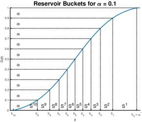
Figure 1: Our reservoir partition. Each consecutive $\alpha$-interval on the CDF defines some subset $\mathcal{S}^{i}$.

It also relies on the following partition of the arms in $\mathcal{W}$ by their expected rewards. Let $m=\lceil 1/\alpha\rceil$. We partition $\mathcal{W}$ into subsets $\mathcal{S}^{i}$ for $1\leq i\leq m$, where $\mathcal{S}^{i}=\{w\in\mathcal{W}:\mu(w)\in]b_{i},b_{i-1}]\}$. The interval boundaries $b_{i}$ are defined so that each subset has measure $\alpha$ under the reservoir distribution $g$, with the possible exception of the subset with smallest expected reward. In particular, $b_{0}=\mu^{*}$ and $b_{i}$ lies at the boundary between subsets $i$ and $i+1$.

$$b_{i}=\left\{\begin{array}[]{ll}\mu^{*}&\text{if $i=0$}\\ G^{-1}(G(b_{i-1})-\alpha)&\text{if $i\geq 1$}\end{array}\right.,$$ (8)

where $\mu^{*}$ is defined in Eq. 2.2. See Figure 1 for an illustration.

In the Bernoulli case, Assumption 2 reduces to $\mu^{*}<1$ (no arm has perfect performance); when the set of possible means $\Theta$ is unbounded it always holds as $G$ has a finite support.

Assumption 2

$\mu^{*}<\sup_{\theta\in\Theta}\theta$.

Theorem 1

Fix some $\alpha,\delta\in]0,1[$. Any $(\alpha,\delta)$-correct algorithm needs an expected sample complexity $\mathds{E}_{\mu}^{M}\left[\tau\right]$ that is lower bounded as follows.

$$\mathds{E}_{\mu}^{M}\left[\tau\right]\geq \left(\frac{1}{\operatorname{d}\left(\mu^{*},b_{2}\right)}+\sum_{i=2}^{m-1}\frac{1}{\operatorname{d}\left(b_{i},\mu^{*}\right)}\right)\log\frac{1}{2.4\delta}.$$

Remark 2

When $\mathcal{W}$ is finite s.t. $|\mathcal{W}|=K$, if we choose a uniform reservoir and let $\alpha=1/K$, then $|\mathcal{S}^{i}|=1$ for all $i$ and our lower bound reduces to the bound obtained by Kaufmann et al. (2016) for best arm identification with $\epsilon=0$. Assuming arm means $\theta_{1}>\theta_{2}\geq\dots\geq\theta_{K}$, one has

$$\mathds{E}_{\mu}^{M}\left[T\right]\geq \left[\frac{1}{\operatorname{d}\left(\theta_{1},\theta_{2}\right)}+\sum_{i=2}^{K}\frac{1}{\operatorname{d}\left(\theta_{i},\theta_{1}\right)}\right]\log\frac{1}{2.4\delta}.$$

3.2 Proof of Theorem 1

The proof relies on the following lemma that expresses a change of measure in an infinite bandit model. Its proof is detailed in Appendix A.

Lemma 3

Let $\lambda:\mathcal{W}\rightarrow\Theta$ be an alternative mean-mapping. Let $T_{i}(t)=\sum_{s=1}^{t}\mathds{1}_{\left(w_{s}\in\mathcal{S}^{i}\right)}$ be the number of times an arm in $\mathcal{S}^{i}$ has been selected. For any stopping time $\sigma$ and any event $C\in H_{\sigma}$,

$$\sum_{i=1}^{m}\mathds{E}_{\mu}^{M}\left[T_{i}(\sigma)\right]\sup_{w\in\mathcal{S}^{i}}\operatorname{d}\left(\mu(w),\lambda(w)\right)\geq\operatorname{kl}\left(\mathbb{P}_{\mu}^{M}\left(C\right),\mathbb{P}_{\lambda}^{M}\left(C\right)\right),$$

where $\operatorname{kl}\left(x,y\right)=x\log(x/y)+(1-x)\log((1-x)/(1-y))$ is the Bernoulli relative entropy.

Let $\tau^{i}=T_{i}(\tau)$ be the (random) number of draws from arms in $\mathcal{S}^{i}$, so $\tau=\sum_{i=1}^{m}\tau^{i}$. Our lower bound on $\mathds{E}_{\mu}^{M}\left[\tau\right]$ follows from bounds on each of the $\mathds{E}_{\mu}^{M}\left[\tau^{i}\right]$. We omit $\mathcal{S}^{m}$ because its measure may be less than $\alpha$. By Assumption 2, there is $\epsilon>0$ such that $\mu^{*}+\epsilon<\sup_{\theta\in\Theta}\theta$. Fix $i$ between $2$ and $m-1$ and define an alternative arm reward mapping $\lambda^{i}(w)$ as follows.

$$\lambda^{i}(w)=\left\{\begin{array}[]{ll}\mu^{*}+\epsilon&\text{if }w\in\mathcal{S}^{i}\\ \mu(w)&\text{otherwise}\end{array}\right.$$ (11)

This mapping induces an alternative reservoir distribution $g^{i}$ under which for all $i<m$, $\mathcal{G}_{M,\lambda^{i}}^{\alpha}=\mathcal{S}^{i}$ because $\mathcal{S}^{i}$ has measure $\alpha$ (as $M$ is unchanged) and under $\lambda^{i}$ the expected rewards of its arms are above all other arms by at least $\epsilon$. Also, by construction $\mathcal{G}_{M,\mu}^{\alpha}=\mathcal{S}^{1}$.

Define the event $C_{\mu}=(\hat{s}_{\tau}\in\mathcal{S}^{1})$. Any $(\alpha,\delta)$-correct algorithm thus satisfies $\mathbb{P}_{\mu}^{M}\left(C_{\mu}\right)\geq 1-\delta$ and $\mathbb{P}_{\lambda}^{M}\left(C_{\mu}\right)\leq\delta$. First using some monotonicity properties of the binary relative entropy $\operatorname{kl}\left(x,y\right)$, one has $\operatorname{kl}\left(\mathbb{P}_{\mu}^{M}\left(C_{\mu}\right),\mathbb{P}_{\lambda^{i}}^{M}\left(C_{\mu}\right)\right)\geq\operatorname{kl}\left(1-\delta,\delta\right)\geq\log\frac{1}{2.4\delta},$ where the second inequality is due to Kaufmann et al. (2016).

Applying Lemma 3 to event $C_{\mu}$ and using the fact that $\lambda^{j}(w)=\mu(w)$ for all $j\neq i$, one obtains $\mathds{E}_{\mu}^{M}\left[T^{i}\right]\sup_{w\in\mathcal{S}^{i}}\operatorname{d}\left(\mu(w),\mu^{*}+\epsilon\right)\geq\log\frac{1}{2.4\delta}.$ Letting $\epsilon$ go to $0$ yields, for all $i\neq 1$,

$$\mathds{E}_{\mu}^{M}\left[\tau^{i}\right]\geq\frac{1}{\sup_{w\in\mathcal{S}^{i}}\operatorname{d}\left(\mu(w),\mu^{*}\right)}\log\left(\frac{1}{2.4\delta}\right),$$

and $\sup_{w\in\mathcal{S}^{i}}\operatorname{d}\left(\mu(w),\mu^{*}\right)\leq\operatorname{d}\left(b_{i},\mu^{*}\right)$ as $\theta\mapsto\operatorname{d}\left(\theta,\mu^{*}\right)$ is decreasing when $\theta<\mu^{*}$.

We now define the alternative mean rewards mapping, for $\epsilon>0$ small enough

$$\lambda^{1}(w)=\left\{\begin{array}[]{ll}b_{2}-\epsilon&\text{if }w\in\mathcal{S}^{1}\\ \mu(w)&\text{otherwise}\end{array}\right.$$ (14)

One has $\mathcal{G}_{M,\mu}^{\alpha}=\mathcal{S}_{1}$ whereas $\mathcal{G}_{M,\lambda^{1}}^{\alpha}=\mathcal{S}_{2}$, hence letting $C_{\mu}=(\hat{s}_{\tau}\in\mathcal{S}_{1})$ satisfies $\mathbb{P}_{\mu}^{M}\left(C_{\mu}\right)\geq 1-\delta$ and $\mathbb{P}_{\lambda^{1}}^{M}\left(C_{\mu}\right)\leq\delta$. Using the same reasoning as before yields

$$\log\left(\frac{1}{2.4\delta}\right)\leq\mathds{E}_{\mu}^{M}\left[\tau^{1}\right]\sup_{w\in\mathcal{S}^{1}}\operatorname{d}\left(\mu(w),b_{2}-\epsilon\right)=\operatorname{d}\left(\mu^{*},b_{2}-\epsilon\right)$$

Letting $\epsilon$ go to zero yields $\mathds{E}_{\mu}^{M}\left[\tau^{1}\right]\geq\displaystyle\frac{1}{\operatorname{d}\left(\mu^{*},b_{2}\right)}\log\left(\frac{1}{2.4\delta}\right)$. $\square$

One can prove an $\epsilon$-relaxed version of this theorem, which provides a lower bound on the number of samples needed to find an arm whose expected reward is within $\epsilon$ of the top-$\alpha$ fraction of arms with probability at least $1-\delta$. When $\epsilon>0$ multiple subsets may contain such arms, and the proof approach above does not work for these subsets. We instead adopt the strategy of Mannor et al. (2004): at most one such subset can have probability greater than $1/2$ of its arms being chosen by the algorithm, so we exclude this subset from our bound. We arrive at the following, which holds when $\mu^{*}+\epsilon$ is in $\Theta$ (i.e. for $\epsilon$ small enough).

Remark 4

Fix some $\alpha,\epsilon,\delta\in]0,1[$, and let $q$ be the number of subsets containing arms within $\epsilon$ of the top $\alpha$ fraction. Any $(\alpha,\epsilon,\delta)$-correct algorithm needs an expected sample complexity $\mathds{E}_{\mu}^{M}\left[\tau\right]$ that is lower bounded as follows.

$$\mathds{E}_{\mu}^{M}\left[\tau\right]\geq \left(\frac{q-1}{\operatorname{d}\left(b_{1}-\epsilon,\mu^{*}+\epsilon\right)}+\sum_{i=q+1}^{m-1}\frac{1}{\operatorname{d}\left(b_{i},\mu^{*}+\epsilon\right)}\right)\log\frac{1}{4\delta}.$$

4 Algorithm and Upper Bound

In this section we assume that $P_{\Theta}=\mathchoice{\left\{p_{\theta},\theta\in\Theta\right\}}{\{p_{\theta},\theta\in\Theta\}}{\{p_{\theta},\theta\in\Theta\}}{\{p_{\theta},\theta\in\Theta\}}$ is a one-parameter exponential family, meaning that there exists some twice differentiable convex function $b(\theta)$ and some reference measure $\nu$ such that $p_{\theta}$ has a density $f_{\theta}$ with respect to $\nu$, where $f_{\theta}(x)=\exp(\theta x-b(\theta)).$ Distributions in an exponential family can indeed be parameterized by their means as $\mu=b^{-1}(\theta)$. We do not make any new assumptions on the reservoir distribution.

Under these assumptions on the arms, we present and analyze a two-phase algorithm called $(\alpha,\epsilon)$-KL-LUCB. We prove the $(\alpha,\epsilon,\delta)$-correctness of this algorithm and a high probability upper bound on its sample complexity in terms of the complexity of the reservoir distribution induced by the arm measure $M$ and the arm reward mapping function $\mu$. We also show how to obtain $(\alpha,\delta)$-correctness under assumptions on the tail of the reservoir.

4.1 The algorithm

0:  $\alpha,\epsilon,\delta>0$

  $n=\frac{1}{\alpha}\ln\frac{2}{\delta}$

  for $a\leftarrow 1$ to $n$ do

     draw arm $w^{a}\sim M$

     sample arm $w^{a}$ once

  end for

  $t=n$ (current number of samples drawn)

  $B(n)=\infty$ (stopping index)

  Compute confidence bounds $U_{a}(n)$ and $L_{a}(n)$

  while $B(t)>\epsilon$ do

     Draw arm $w^{\hat{a}(t)}$ and $w^{\hat{b}(t)}$

     $t=t+2$

     Update confidence bounds, compute $\hat{a}(t)$ and $\hat{b}(t)$

     $B(t)=U_{\hat{b}(t)}(t)-L_{\hat{a}(t)}(t)$

  end while

  return $w^{\hat{a}(t)}$

Algorithm 2 $(\alpha,\epsilon)$-KL-LUCB

$(\alpha,\epsilon)$-KL-LUCB, presented as Algorithm 2, is a two-phase algorithm. It first queries $n=\frac{1}{\alpha}\log\frac{2}{\delta}$ arms $w^{1},\dots,w^{n}$ from $M$, the measure over $\mathcal{W}$, and then runs the KL-LUCB algorithm (Kaufmann and Kalyanakrishnan, 2013) on the queried arms. KL-LUCB identifies the $m$-best arms in a multi-armed bandit model, up to some $\epsilon>0$. We use it with $m=1$. This algorithm adaptively selects pairs of arms to sample from based on confidence intervals on the means of the arms. These confidence intervals rely on some exploration rate

$$\beta(t,\delta):=\log(k_{1}nt^{\gamma}/\delta),$$ (15)

for constants $\gamma>1$ and $k_{1}>2(1+\frac{1}{\gamma}-1)$. The upper and lower confidence bounds are

$$U_{a}(t) :=\max\mathchoice{\left\{\theta\in\Theta:N_{a}(t)\operatorname{d}\left(\hat{p}_{a}(t),\theta\right)\leq\beta(t,\delta)\right\}}{\{\theta\in\Theta:N_{a}(t)\operatorname{d}\left(\hat{p}_{a}(t),\theta\right)\leq\beta(t,\delta)\}}{\{\theta\in\Theta:N_{a}(t)\operatorname{d}\left(\hat{p}_{a}(t),\theta\right)\leq\beta(t,\delta)\}}{\{\theta\in\Theta:N_{a}(t)\operatorname{d}\left(\hat{p}_{a}(t),\theta\right)\leq\beta(t,\delta)\}}$$ (16)

$$L_{a}(t) :=\min\mathchoice{\left\{\theta\in\Theta:N_{a}(t)\operatorname{d}\left(\hat{p}_{a}(t),\theta\right)\leq\beta(t,\delta)\right\}}{\{\theta\in\Theta:N_{a}(t)\operatorname{d}\left(\hat{p}_{a}(t),\theta\right)\leq\beta(t,\delta)\}}{\{\theta\in\Theta:N_{a}(t)\operatorname{d}\left(\hat{p}_{a}(t),\theta\right)\leq\beta(t,\delta)\}}{\{\theta\in\Theta:N_{a}(t)\operatorname{d}\left(\hat{p}_{a}(t),\theta\right)\leq\beta(t,\delta)\}},$$ (17)

where $N_{a}(t)=\sum_{s=1}^{t}\mathds{1}_{\left(W_{s}=w^{a}\right)}$ is the number of times arm $w^{a}$ was sampled by round $t$ and $\hat{p}_{a}(t)=\frac{1}{N_{a}(t)}\sum_{s=1}^{t}\mathds{1}_{\left(W_{s}=w^{a}\right)}Z_{s}$ is the empirical mean reward of arm $w^{a}$ at round $t$, where $Z_{s}$ is an i.i.d. draw from arm $W_{s}$, with distribution $p_{\mu(W_{s})}$. Recall that $\operatorname{d}\left(\mu_{1},\mu_{2}\right)$ is the KL divergence between arm distributions parameterized by their means $\mu_{1}$ and $\mu_{2}$.

For each queried arm $w^{a}$, the algorithm maintains a confidence interval $\mathcal{I}_{a}(t)=[L_{a}(t),U_{a}(t)]$ on $\mu(w^{a})$, and at any even round $t$ selects two arm indexes: (1) the empirical best arm $\hat{a}(t)\in{\operatorname*{argmax}}_{a=1,\dots,n}\ \hat{p}_{a}(t)$, and (2) the arm among the empirical worst arms that is most likely to be mistaken with $\hat{a}(t)$, $\hat{b}(t)={\operatorname*{argmax}}_{a\neq\hat{a}(t)}\ U_{a}(t)$. The two arms are sampled: $W_{t}=w^{\hat{a}(t)}$ and $W_{t+1}=w^{\hat{b}(t)}$ and the confidence intervals are updated. The algorithm terminates when the overlap between the associated confidence intervals is smaller than some $\epsilon>0$: $\tau=\inf\mathchoice{\left\{t\in\mathbb{N}^{*}:L_{\hat{a}(t)}(t)>\max_{a\neq\hat{a}(t)}U_{a}(t)+\epsilon\right\}}{\{t\in\mathbb{N}^{*}:L_{\hat{a}(t)}(t)>\max_{a\neq\hat{a}(t)}U_{a}(t)+\epsilon\}}{\{t\in\mathbb{N}^{*}:L_{\hat{a}(t)}(t)>\max_{a\neq\hat{a}(t)}U_{a}(t)+\epsilon\}}{\{t\in\mathbb{N}^{*}:L_{\hat{a}(t)}(t)>\max_{a\neq\hat{a}(t)}U_{a}(t)+\epsilon\}}.$ The recommendation rule is $\hat{s}_{\tau}=w^{\hat{a}(t)}$.

4.2 $(\alpha,\epsilon,\delta)$-Correctness

For the algorithm to be $(\alpha,\epsilon,\delta)$-correct, it is sufficient that the following two events occur:

• $A$ is the event that some $w^{a}$ was drawn from the top-$\alpha$ fraction of the reservoir.

• $B$ is the event that the KL-LUCB algorithm succeeds in identifying an arm within $\epsilon$ of the best arm among the $n$ arms drawn in the initialization phase.

Indeed, on $A\cap B$ the recommended arm $\hat{s}_{\tau}=w^{\hat{a}(\tau)}$ satisfies $\mu(\hat{s}_{\tau})>\max_{a}\mu(w^{a})-\epsilon\geq G^{-1}(1-\alpha)-\epsilon,$ hence $\hat{s}_{\tau}$ belongs to the top-$\alpha$ fraction, up to $\epsilon$. We prove in Appendix B that $\mathbb{P}\left(A^{\complement}\right)\leq\delta/2$ and $\mathbb{P}\left(B^{\complement}\right)\leq\delta/2$, which yields the following result.

Lemma 5

With $\beta(t,\delta)$ defined in (15), $(\alpha,\epsilon)$-KL-LUCB returns an arm from $\mathcal{G}_{M,\mu}^{\alpha,\epsilon}$ with probability at least $1-\delta$.

It follows that when the parameter $\epsilon$ is chosen small enough, e.g., $\epsilon<G^{-1}\left(1-\frac{\alpha}{2}\right)-G^{-1}\left(1-{\alpha}\right),$ $(\alpha,\epsilon)$-KL-LUCB is $(\alpha/2,\delta)$-correct. For example, under the tail assumption 3, $\epsilon$ can be chosen of order $c\alpha^{1/\beta}$. However, when nothing is known about the reservoir distribution (e.g. it may not even be smooth) we are not aware of an algorithm to choose $\epsilon$ to provide a $(\alpha,\delta)$-correctness guarantee.

4.3 Sample Complexity of $(\alpha,\epsilon)$-KL-LUCB

Recall the partition of $\mathcal{W}$ into subsets $\mathcal{S}^{i}$ of measure $\alpha$ for $1\leq i\leq m$, where $\mathcal{S}^{i}=\mathchoice{\left\{w\in\mathcal{W}:\mu(w)\in]b_{i},b_{i-1}]\right\}}{\{w\in\mathcal{W}:\mu(w)\in]b_{i},b_{i-1}]\}}{\{w\in\mathcal{W}:\mu(w)\in]b_{i},b_{i-1}]\}}{\{w\in\mathcal{W}:\mu(w)\in]b_{i},b_{i-1}]\}}$. We define our sample complexity bound in terms of the complexity term:

$$\overline{H}_{\alpha,\epsilon}=\frac{2}{\epsilon^{2}}+\sum_{i=2}^{m}\frac{1}{\max(\epsilon^{2}/2,\operatorname{d^{*}}\left(b_{i-1},b_{1}\right))},$$ (18)

where $\operatorname{d^{*}}\left(p,q\right)$ is the Chernoff information between two reward distributions parameterized by their means $p$ and $q$. This quantity is closely related to the KL-divergence: it is defined as $\operatorname{d^{*}}\left(p,q\right)=\operatorname{d}\left(z^{*},p\right)$ where $z^{*}$ is the unique solution in $z$ to $\operatorname{d}\left(z,p\right)=\operatorname{d}\left(z,q\right)$.

Let the random variable $\tau$ be the number of samples used by $(\alpha,\epsilon)$-KL-LUCB. The following upper bound on $\tau$ holds.

Theorem 6

Let $\alpha,\delta$ such that $0<\delta\leq\alpha\leq 1/3$. The $(\alpha,\epsilon)$-KL-LUCB algorithm with exploration rate $\beta(t,\delta)$ defined by (15) and a parameter $\epsilon>0$ is $(\alpha,\epsilon,\delta)$-correct and satisfies, with probability at least $1-7\delta$,

$$\tau\leq 12C_{0}(\gamma)\overline{H}_{\alpha,\epsilon}\log^{2}\frac{1}{\delta}+o\left(\log^{2}\frac{1}{\delta}\right),$$

with $C_{0}(\gamma)$ such that $C_{0}(\gamma)\geq\gamma\log(C_{0}(\gamma))+1+\frac{\gamma}{e}$.

Theorem 6 only presents the leading term in $\delta$ (when $\delta$ goes to zero) of the sample complexity upper bound, but an explicit upper bound can be extracted from the proof of Theorem 6, given in Appendix D.

4.4 Comparison and Discussion

Our $\epsilon$-relaxed bounds simplify, for appropriate constants $c_{1},c_{2}$ and small enough $\epsilon$, to

$$\mathds{E}_{\mu}^{M}\left[\tau\right] \geq c_{1}\left(\frac{1}{\operatorname{d}\left(b_{1}-\epsilon,b_{0}+\epsilon\right)}+\sum_{i=3}^{m-1}\frac{1}{\operatorname{d}\left(b_{i},b_{0}+\epsilon\right)}\right)\log\frac{1}{\delta},$$

$$\tau \leq c_{2}\left(\frac{4}{\epsilon^{2}}+\sum_{i=2}^{m-1}\frac{1}{\operatorname{d^{*}}\left(b_{i},b_{1}\right)}\right)\log^{2}\frac{1}{\delta}.$$

A log factor separates our bounds, and the upper bound complexity term is slightly larger than that in the lower bound. KL-divergence in the lower bound is of comparable scale to Chernoff information in the upper bound: in the Bernoulli case one has $\frac{(\mu^{*}-x)^{2}}{2}<\operatorname{d^{*}}\left(x,\mu^{*}\right)<\operatorname{d}\left(x,\mu^{*}\right)<\frac{(\mu^{*}-x)^{2}}{\mu^{*}(1-\mu^{*})}.$ However, for $i\neq 1$, $\operatorname{d^{*}}\left(b_{i},b_{1}\right)$ is slightly smaller than $\operatorname{d}\left(b_{i},b_{0}+\epsilon\right)$, while $\epsilon^{2}$ is smaller than $\operatorname{d}\left(b_{1}-\epsilon,b_{0}+\epsilon\right)$. These differences are reduced as $\alpha$ is decreased.

When $\delta$ is not too small, the extra $\log\frac{1}{\delta}$ factor is small compared to the constants in our upper bound. It is well-established for finite bandit models that for a wide variety of algorithms the sample complexity scales like $\log\frac{1}{\delta}$. The additional log factor comes from the fact that each phase of our algorithm needs a $\delta$-correctness guarantee. In our first phase, we choose a number of arms to draw from the reservoir without drawing any rewards from those arms. In the second phase, we observe rewards from our arms without drawing any new arms from the reservoir. It is an interesting open question to prove whether in any such two-phase algorithm the $\log^{2}\frac{1}{\delta}$ term is avoidable. It is not hard to show that the first phase must draw at least $\frac{c}{\alpha}\log\frac{1}{\delta}$ arms for some constant $c$ in order to obtain a single arm from the top-$\alpha$ fraction with high probability, but the expected number of arms in the top-$\alpha$ fraction is already $c\log\frac{1}{\delta}$ in this case. The second phase can be reduced to a problem of finding one of the top $m$ arms, or of finding one arm above the unknown threshold $G^{-1}(1-\alpha)$, but we are not aware of a lower bound on these problems even for the finite case.

Despite all this, it seems likely that a one-phase algorithm can avoid the quadratic dependence on $\log\frac{1}{\delta}$. Indeed, Jamieson et al. (2016) provides such an algorithm for the special case of reservoirs involving just two expected rewards. They employ a subroutine which returns the target coin with constant probability by drawing a number of coins that does not depend on $\delta$. They wrap this subroutine in a $\delta$-correct algorithm which iteratively considers progressively more challenging reservoirs, terminating when a target coin is identified. We agree with the authors that adapting this approach for general reservoirs is an interesting research direction. However their method relies on the special shape of their reservoir and it is not immediately clear how it might be generalized.

5 Conclusion

In contrast with previous approaches to bandit models, we have limited consideration to changes of distribution which change only the mean mapping $\mu$ and not the measure $M$ over arms $\mathcal{W}$. This allows us to analyze infinite bandit models without a need to integrate over the full reservoir distribution, so we can prove results for reservoirs which are not even smooth. We proved a lower bound on the sample complexity of the problem, and we introduced an algorithm with an upper bound within a log factor of our lower bound.

An interesting future direction is to study improved algorithms, namely one-phase algorithms which alternate between sampling arms to estimate the reservoir and drawing new arms to obtain better arms with higher confidence. These algorithms might be able to have only a $\log\frac{1}{\delta}$ instead of $\log^{2}\frac{1}{\delta}$ dependency in the upper bound. In practice, however, the algorithm we present exhibits good empirical performance.

Acknowledgement.

We thank Virgil Pavlu for the fruitful discussions and his efforts that made this project better. E. Kaufmann acknowledges the support of the French Agence Nationale de la Recherche (ANR), under grant ANR-16-CE40-0002 (project BADASS).

A Changes of distribution in infinite bandit models

A.1 Proof of Lemma 3

We describe in this section the key results that allow us to adapt changes of distribution arguments to the infinite bandit setting. Lemma 3 follows easily from Lemma 7 and Lemma 8 that are stated below and proved in the next two sections.

All the regret or sample complexity lower bounds in bandit models rely on change of distributions arguments (see, e.g. [27, 7, 2]). A change of distribution relates the probability of an event under a given bandit model to the probability of that event under an alternative bandit model, that is “not too far” from the initial model but under which the performance of the algorithm is supposed to be completely different. [28, 25] recently found an elegant formulation for such a change of distribution in terms of the expected log-likelihood ratio and we explain below how we generalize these tools to the infinite bandit model.

Given an infinite bandit model $(M,\mu)$, one may consider an alternative bandit model $(M,\lambda)$ in which the measure $M$ is similar but the mean function is different: $\lambda\neq\mu$. As mentioned in Section 2.1, we consider strategies such that $\mathbb{P}_{\mu}^{M}\left(W_{t}|H_{T-1}\right)$ is independent from $\mu$. Hence, defining the log-likelihood ratio between $(M,\mu)$ and $(M,\lambda)$ at round $t$ as $L_{\mu,\lambda}(t)=\log(\ell(H_{t};\mu,M)/\ell(H_{t};\lambda,M))$, where the likelihood is defined in (1), one has

$$L_{\mu,\lambda}(T) =\sum_{t=1}^{T}\log\frac{f_{\mu(W_{t})}(Z_{t})}{f_{\lambda(W_{t})}(Z_{t})}.$$ (19)

The following result generalizes Lemma 1 in [25] to the infinite bandit model. It permits to relate the expected log-likelihood ratio to the probability of any event under the two different models.

Lemma 7

Let $\sigma$ be a stopping time and $\mu$ and $\lambda$ be two reward mappings. For any event $C$ in $H_{\sigma}$,

$$\mathds{E}_{\mu}^{M}\left[L_{\mu,\lambda}(\sigma)\right]\geq\operatorname{kl}\left(\mathbb{P}_{\mu}^{M}\left(C\right),\mathbb{P}_{\lambda}^{M}\left(C\right)\right),$$

where $\operatorname{kl}\left(x,y\right)=x\log(x/y)+(1-x)\log((1-x)/(1-y))$ is the Bernoulli relative entropy.

The next result provides an upper bound on the expected log-likelihood ratio. While in a classic multi-armed bandit model, the log-likelihood can be expressed as a sum that features the expected number of draws of each arm, such a quantity would not be defined in the infinite bandit model. Hence, we need to introduce a partition of $\mathcal{W}$.

Lemma 8

Fix $\mathcal{S}_{1},\dots,\mathcal{S}_{m}$ a partition of $\mathcal{W}$ and let $T_{i}(t)=\sum_{s=1}^{t}\mathds{1}_{\left(w_{s}\in\mathcal{S}^{i}\right)}$ be the number of times an arm in $\mathcal{S}^{i}$ has been selected. For any stopping time $\sigma$,

$$\mathds{E}_{\mu}^{M}\left[L_{\mu,\lambda}(\sigma)\right]\leq\sum_{i=1}^{m}\mathds{E}_{\mu}^{M}\left[T_{i}(\sigma)\right]\sup_{w\in\mathcal{S}^{i}}\operatorname{d}\left(\mu(w),\lambda(w)\right).$$

A.2 Proof of Lemma 7

The proof for the infinite case follows the argument by [25] for the finite case. First, the conditional Jensen’s inequality is applied, given the convexity of $\exp(-x)$. The expectation derivations hold for our infinite arms case without modification. The only necessary statement for which the finite case proof needs updating, $\mathbb{P}_{\lambda}^{M}\left(C\right)=\mathds{E}_{\mu}^{M}\left[\mathds{1}_{\left(C\right)}\exp(-L_{\mu,\lambda}(\sigma))\right]$, is proven for our infinite case setting as Lemma 9.

Lemma 9

Let $\mu$ and $\lambda$ be two arm reward mappings, $L_{\mu,\lambda}(T)$ be the log likelihood ratio defined in (19) and $C$ be an (event) subset of histories of length $T$. Then

$$\mathbb{P}_{\lambda}^{M}\left(C\right)=\mathds{E}_{\mu}^{M}\left[\mathds{1}_{\left(C\right)}\cdot\exp(-L_{\mu,\lambda}(T))\right]$$

Proof of Lemma 9.

Let $\ell(H_{T};\mu,M)$ be the likelihood function defined in (1). We introduce furthermore the notation $h_{t}=(W_{1},Z_{1},\dots,W_{t},Z_{t})$, $\bm{w}_{T}=(W_{1},\dots,W_{T})$ and $\bm{z}_{T}=(Z_{1},\dots,Z_{T})$. Recall that a strategy is such that conditional density of $W_{t}$ given $H_{t-1}$ does not depend on the mean reward mapping but only on the reservoir distribution: we denote it by $\mathbb{P}_{M}(W_{t}|H_{t-1})$. The proof of Lemma 9 follows from the following inequalities.

$$\mathbb{P}_{\lambda}^{M}\left(C\right)=\mathds{E}_{\lambda}^{M}\left[\mathds{1}_{\left(C\right)}\right] =\int\mathds{1}_{\left(C\right)}(H_{T})\ell(H_{T};\lambda,M)\mathop{}\!\mathrm{d}H_{T}$$

$$=\int\mathds{1}_{\left(C\right)}(h_{T})\prod_{t=1}^{T}f_{\lambda(W_{t})}(Z_{t})\mathbb{P}_{M}(W_{t}|h_{t-1})\mathop{}\!\mathrm{d}\bm{w}_{T}\mathop{}\!\mathrm{d}\bm{z}_{T}$$

$$=\int\mathds{1}_{\left(C\right)}(h_{T})\prod_{t=1}^{T}\frac{f_{\lambda(W_{t})}(Z_{t})}{f_{\mu(W_{t})}(Z_{t})}\prod_{t=1}^{T}f_{\mu(W_{t})}(Z_{t})\mathbb{P}_{M}(W_{t}|h_{t-1})\mathop{}\!\mathrm{d}\bm{w}_{T}\mathop{}\!\mathrm{d}\bm{z}_{T}$$

$$=\int\mathds{1}_{\left(C\right)}(H_{T})\prod_{t=1}^{T}\frac{f_{\lambda(W_{t})}(Z_{t})}{f_{\mu(W_{t})}(Z_{t})}\ell(H_{T};\mu,M)\mathop{}\!\mathrm{d}H_{T}$$

$$=\mathds{E}_{\mu}^{M}\left[\mathds{1}_{\left(C\right)}\cdot\prod_{t=1}^{T}\frac{f_{\lambda(W_{t})}(Z_{t})}{f_{\mu(W_{t})}(Z_{t})}\right].$$

$\square$

A.3 Proof of Lemma 8

The proof follows from the following inequalities.

$$\mathds{E}_{\mu}^{M}\left[L_{\mu,\lambda}(\sigma)\right]$$

$$=\mathds{E}_{\mu}^{M}\left[\sum_{t=1}^{\infty}\mathds{E}_{\mu}^{M}\left[\left.\mathds{1}_{\left(\sigma\geq t-1\right)}\log\frac{f_{\mu(W_{t})}(Z_{t})}{f_{\lambda(W_{t})}(Z_{t})}\right|H_{t-1}\right]\right]$$

$$=\mathds{E}_{\mu}^{M}\left[\sum_{t=1}^{\infty}\mathds{1}_{\left(\sigma\geq t-1\right)}\operatorname{d}\left(\mu(W_{t}),\lambda(W_{t})\right)\right]$$

$$\leq\mathds{E}_{\mu}^{M}\left[\sum_{i=1}^{m}\sum_{t=1}^{\sigma}\mathds{1}_{\left(W_{t}\in\mathcal{S}^{i}\right)}\sup_{w\in\mathcal{S}^{i}}\operatorname{d}\left(\mu(w),\lambda(w)\right)\right]$$

B Proof of Lemma 5

Letting

$$A =\left(\exists a\leq n:\mu(w^{a})>G^{-1}(1-\alpha)\right)$$

$$B =\left(\mu_{\hat{a}(\tau)}\geq\max_{a}\mu_{a}-\epsilon\right),$$

Lemma 5 follows from the fact that $\mathbb{P}\left(A^{\complement}\right)\leq\frac{\delta}{2}$ and $\mathbb{P}\left(B^{\complement}\right)\leq\frac{\delta}{2}$, that we now prove.

First, by definition of the reservoir distribution $G$ and the fact that $\mu(W^{t})$ are i.i.d. samples from it, one has

$$\mathbb{P}\left(A^{\complement}\right) =\mathbb{P}\left(\bigcap_{a=1}^{n}\left(\mu(w^{a})\leq G^{-1}(1-\alpha)\right)\right)=\left(1-\alpha\right)^{n}$$

$$=\exp\left(-n\log\left(\frac{1}{1-\alpha}\right)\right)$$

$$=\exp\left(-\log\left(\frac{2}{\delta}\right)\frac{1}{\alpha}\log\left(\frac{1}{1-\alpha}\right)\right)\leq\frac{\delta}{2},$$

using that $-\log(1-x)>x$.

The upper bound on $\mathbb{P}\left(B^{\complement}\right)$ follows the same lines as that of the correctness of the KL-LUCB algorithm [24], however note that we are able to use a smaller exploration rate compared to this work. Abusing notation slightly we let $\mu_{a}:=\mu(w^{a})$, and letting $(1)=\operatorname*{argmax}_{a}\mu_{a}$ we have

$$B^{\complement} \subseteq(\exists t\in\mathbb{N}:\mu_{(1)}>U_{(1)}(t))\!\!\!\!\!\bigcup_{a:\mu_{a}<\mu_{(1)}-\epsilon}\!\!\!\!\!\!\!\!(\exists t\in\mathbb{N}:L_{a}(t)>\mu_{a}).$$

Let $\operatorname{d}^{-}(x,y):=\operatorname{d}\left(x,y\right)\mathds{1}_{\left(x>y\right)}$. For each $a$, $\mathbb{P}\left(\exists t\in\mathbb{N}:L_{a}(t)>\mu_{a}|\mu_{a}\right)$ is upper bounded by

$$\mathbb{P}\left(\exists t\in\mathbb{N}:N_{a}(t)\operatorname{d}^{-}(\hat{p}_{a}(t),\mu_{a})>\beta(t,\delta)\right)$$

$$\leq\mathbb{P}\left(\exists t\in\mathbb{N}:N_{a}(t)\operatorname{d}^{-}(\hat{p}_{a}(t),\mu_{a})>\beta(N_{a}(t),\delta)\right)$$

$$\leq\mathbb{P}\left(\exists s\in\mathbb{N}:s\operatorname{d}^{-}(\hat{p}_{a}(t),\mu_{a})>\beta(s,\delta)\right)$$

$$\leq\sum_{s=1}^{\infty}\exp(-\beta(s,\delta))\leq\frac{\delta}{k_{1}n}\sum_{t=1}^{\infty}\frac{1}{t^{\gamma}}\leq\frac{\delta}{2n},$$

where we use a union bound together with Chernoff’s inequality and the fact that $k_{1}$ is chosen to be larger than $2\sum_{t}\frac{1}{t^{\gamma}}$. Similar reasoning shows that

$$\mathbb{P}\left(\exists t\in\mathbb{N}:\mu_{(1)}>U_{(1)}(t)\right)\leq\frac{\delta}{2n},$$

and a union bound yields $\mathbb{P}\left(B^{\complement}\right)\leq\frac{\delta}{2}$.

C Proof of Lemma 11

For every $i$, let $\mathcal{R}_{i}$ be the set of arms $a\in\{1,\dots,n\}$ such that $w^{a}\in\mathcal{S}^{i}$. Letting $Y^{i}_{a}=\mathds{1}_{\left(w^{a}\in\mathcal{S}^{i}\right)}$, as $M(\mathcal{S}^{i})=\alpha$, $(Y^{i}_{a})_{a}$ is i.i.d. with a Bernoulli distribution of parameter $\alpha$ and $|\mathcal{R}_{i}|=\sum_{a=1}^{n}Y^{i}_{a}$.

Using Chernoff’s inequality for Bernoulli random variables yields

$$\mathbb{P}\left(|\mathcal{R}_{i}|>6\log(1/\delta)\right)=\mathbb{P}\left(|\mathcal{R}_{i}|>3\alpha n\right)$$

$$=\mathbb{P}\left(\frac{1}{n}\sum_{a=1}^{n}Y^{i}_{a}>3\alpha\right)\leq\exp\left\{-n\operatorname{kl}\left(3\alpha,\alpha\right)\right\},$$

where $\operatorname{kl}\left(x,y\right)=x\log(x/y)+(1-x)\log((1-x)/(1-y))$ is the binary relative entropy.

Using Lemma 10 below for $\beta=2$, if $\alpha\leq 1/3$ it holds that

$$\operatorname{kl}\left(3\alpha,\alpha\right)\geq(3\log 3-2)\alpha>\alpha$$

and, using again the definition of $n$,

$$\mathbb{P}\left(|\mathcal{R}_{i}|>6\log(1/\delta)\right)\leq\exp\left\{-2\log(1/\delta)\right\}=\delta^{2}.$$

Using a union bound on the $m$ subsets $\mathcal{S}^{i}$, and the fact that $m\leq 1/\alpha$ and $\delta\leq\alpha$, one has

$$\mathbb{P}\left(C^{\complement}\right)\leq m\delta^{2}\leq\frac{\delta^{2}}{\alpha}\leq\delta,$$

which concludes the proof.

Lemma 10

Let $\beta>-1$. For all $\alpha\leq\frac{1}{1+\beta}$,

$$\operatorname{kl}\left((1+\beta)\alpha,\alpha\right)\geq((1+\beta)\log(1+\beta)-\beta)\alpha.$$

This inequality is optimal in the first order in the sense that its two members are equivalent when $\alpha$ goes to zero.

Proof of Lemma 10.

By definition

$$\operatorname{kl}\left((1+\beta)\alpha,\alpha\right)= (1+\beta)\alpha\log(1+\beta)$$

$$+(1-(1+\beta)\alpha)\log\left(\frac{1-(1+\beta)\alpha}{1-\alpha}\right)$$

$$= (1+\beta)\alpha\log(1+\beta)$$

$$+(1-(1+\beta)\alpha)\log\left(1-\frac{\beta\alpha}{1-\alpha}\right)$$

Now, using the fact that $1-(1-\beta)\alpha>0$ for $\alpha\leq 1/(1+\beta)$ and the following inequality

$$\forall x>-1,\ \ \log(1+x)\geq\frac{x}{1+x}$$

one obtains

$$\operatorname{kl}\left((1+\beta)\alpha,\alpha\right)\geq (1+\beta)\alpha\log(1+\beta)$$

$$+(1-(1+\beta)\alpha)\frac{-\beta\alpha}{1-\alpha-\beta\alpha}$$

$$= \alpha\left((1+\beta)\log(1+\beta)-\beta\right)$$

$\square$

D Proof of Theorem 6

We let $\mu_{a}:=\mu(w^{a})$ and denote by $\bm{\mu}=(\mu_{1},\dots,\mu_{n})$ the means of the $n$ arms that have been queried, sorted in decreasing order.

In addition to events $A$ and $B$ defined in Section 4.2, we introduce the event $C$ that for every subset $i\leq m$, at most $6\log\frac{1}{\delta}$ arms belong to $\mathcal{S}^{i}$:

$$C=\bigcap_{i=1,\dots,m}\left\{|\{a\leq n:w^{a}\in\mathcal{S}^{i}\}|\leq 6\log({1}/{\delta})\right\}$$ (20)

We prove the following in Appendix C.

Lemma 11

If $\delta\leq\alpha\leq 1/3$, $\mathbb{P}\left(C\right)\geq 1-\delta$.

For all $t\in\mathbb{N}$ we introduce the event

$$W_{t}=\bigcap_{1\leq a\leq n}(L_{a}(t)\leq\mu_{a}\leq U_{a}(t))$$ (21)

and define $W=\cap_{t\in\mathbb{N}^{*}}W_{t}$. By the same argument as the one used in the proof of Lemma 5 (see Appendix B), one can show that $\mathbb{P}\left(W\right)\geq 1-2\delta.$

Fix $c\in[\mu_{2},\mu_{1}]$. Our analysis relies on the following crucial statement.

Proposition 12 ([24])

Let $\tilde{\beta}_{a}(t):=\sqrt{\frac{\beta(t,\delta)}{2N_{a}(t)}}$. If $W_{t}$ holds and $(U_{\hat{b}(t)}-L_{\hat{a}(t)}>\epsilon)$ then there exists $a\in\{\hat{a}(t),\hat{b}(t)\}$ such that

$$c\in\mathcal{I}_{a}(t)\text{ and }\tilde{\beta}_{a}(t)>{\epsilon}/{2}.$$ (22)

Fixing some integer $T\in\mathbb{N}$, we now upper bound $\tau$ on the event $\mathcal{E}:=A\cap B\cap C\cap W$.

$$\min(\tau,T)\leq\sum_{t=1}^{T}\mathds{1}_{\left(\tau>t\right)}=n+2\sum_{\begin{subarray}{c}t\in n+2\mathbb{N}\\ t\leq T\end{subarray}}\mathds{1}_{\left(\tau>t\right)}$$

$$\leq n+2\sum_{\begin{subarray}{c}t\in n+2\mathbb{N}\\ t\leq T\end{subarray}}\mathds{1}_{\left(U_{\hat{b}(t)}-L_{\hat{a}(t)}>\epsilon\right)}$$

$$\leq n+2\sum_{\begin{subarray}{c}t\in n+2\mathbb{N}\\ t\leq T\end{subarray}}\mathds{1}_{\left(\exists a\in\{\hat{a}(t),\hat{b}(t)\}:c\in\mathcal{I}_{a}(t),\tilde{\beta}_{a}(t)>\epsilon/2\right)},$$

using Proposition 12 and the fact that W holds. To ease the notation, we let $\mathcal{S}_{t}=\{\hat{a}(t),\hat{b}(t)\}$ be the set of drawn arms at round $t$. Letting $\mathcal{A}_{\epsilon}=\mathchoice{\left\{a:\operatorname{d^{*}}\left(\mu_{a},c\right)<\epsilon^{2}/2\right\}}{\{a:\operatorname{d^{*}}\left(\mu_{a},c\right)<\epsilon^{2}/2\}}{\{a:\operatorname{d^{*}}\left(\mu_{a},c\right)<\epsilon^{2}/2\}}{\{a:\operatorname{d^{*}}\left(\mu_{a},c\right)<\epsilon^{2}/2\}}$ and noting that $\tilde{\beta}_{a}(t)>\epsilon/2\iff N_{a}(t)<\beta(t,\delta)/(\epsilon^{2}/2)$,

$$\min(\tau,T)\leq n+2\!\sum_{a\in\mathcal{A}_{\epsilon}}\!\sum_{\begin{subarray}{c}t\in n+2\mathbb{N}\\ t\leq T\end{subarray}}\!\!\!\mathds{1}_{\left(a\in\mathcal{S}_{t}\right)}\mathds{1}_{\left(N_{a}(t)<\beta(T,\delta)/(\epsilon^{2}/2)\right)}$$

$$\hskip 28.45274pt+2\sum_{a\in\mathcal{A}_{\epsilon}^{\complement}}\sum_{\begin{subarray}{c}t\in n+2\mathbb{N}\\ t\leq T\end{subarray}}\mathds{1}_{\left(a\in\mathcal{S}_{t}\right)}\mathds{1}_{\left(N_{a}(t)\operatorname{d}\left(\hat{p}_{a}(t),c\right)\leq\beta(T,\delta))\right)}$$

Now defining the event

$$G_{T}^{a}=\!\!\!\!\!\bigcup_{\begin{subarray}{c}t\in n+2\mathbb{N}\\ t\leq T\end{subarray}}\!\!\left\{\!N_{a}(t)>\!\frac{\beta(T,\delta)}{\operatorname{d^{*}}\left(\mu_{a},c\right)},N_{a}(t)\operatorname{d}\left(\hat{p}_{a}(t),c\right)\!\leq\!\beta(T,\delta)\!\right\}$$

From Lemma 1 in [24],

$$\mathbb{P}\left(G_{T}^{a}|\bm{\mu}\right)\leq\frac{1}{\operatorname{d^{*}}\left(\mu_{a},c\right)}\exp(-\beta(T,\delta)).$$ (23)

Introducing $\mathcal{F}_{T}=\cap_{a\in\mathcal{A}_{\epsilon}^{\complement}}(G_{T}^{a})^{\complement}$, one can further upper bound $\tau$ on $\mathcal{E}\cap\mathcal{F}_{T}$ as

$$\min(\tau,T)\leq n+2\!\sum_{a\in\mathcal{A}_{\epsilon}}\!\sum_{\begin{subarray}{c}t\in n+2\mathbb{N}\\ t\leq T\end{subarray}}\!\!\!\!\mathds{1}_{\left(a\in\mathcal{S}_{t}\right)}\mathds{1}_{\left(N_{a}(t)<\beta(T,\delta)/(\epsilon^{2}/2)\right)}$$

$$\hskip 28.45274pt+2\sum_{a\in\mathcal{A}_{\epsilon}^{\complement}}\sum_{\begin{subarray}{c}t\in n+2\mathbb{N}\\ t\leq T\end{subarray}}\mathds{1}_{\left(a\in\mathcal{S}_{t}\right)}\mathds{1}_{\left(N_{a}(t)<\beta(T,\delta)/\operatorname{d^{*}}\left(\mu_{a},c\right)\right)}$$

$$\hskip 28.45274pt\leq n+2\underbrace{\left[\sum_{a\in\mathcal{A}_{\epsilon}}\frac{2}{\epsilon^{2}}+\sum_{a\in\mathcal{A}_{\epsilon}^{\complement}}\frac{1}{\operatorname{d^{*}}\left(\mu_{a},c\right)}\right]}_{=:H(\bm{\mu},c,\epsilon)}\beta(T,\delta).$$

We now provide a deterministic upper bound on $H(\bm{\mu},c,\epsilon)$, by summing over the arms in the different subsets $\mathcal{S}^{i}$. Let $q$ be the number of subsets containing arms within $\mathcal{A}_{\epsilon}$. We choose $c$ such that $c>G^{-1}(1-\alpha)=b_{1}$ (such a choice is possible as $\mu_{1}>G^{-1}(1-\alpha)$ as event $A$ holds) and note that $\mathcal{A}_{\epsilon}\subseteq\cup_{i\leq q}\mathcal{S}_{i}$. One has

$$H(\bm{\mu},c,\epsilon)\!\! \leq \!\!\!\!\!\sum_{i=1}^{q}\sum_{a:w_{a}\in\mathcal{S}^{i}}\frac{2}{\epsilon^{2}}+\sum_{i=q+1}^{m}\sum_{a:w_{a}\in\mathcal{S}^{i}}\!\!\frac{1}{\operatorname{d^{*}}\left(\mu_{a},G^{-1}(1-\alpha)\right)}$$

$$\leq \!\!6\overline{H}_{\alpha,\epsilon}\log(1/\delta),$$

using that event $C$ holds and each $\mathcal{S}^{i}$ contains at least $6\log(1/\delta)$ arms. Hence on $\mathcal{E}\cap\mathcal{F}_{T}$,

$$\min(\tau,T)\leq n+12\overline{H}_{\alpha,\epsilon}\log(1/\delta)\beta(T,\delta).$$

Applying this to $T=T^{*}$ where

$$T^{*}:=\inf\{T\in\mathbb{N}:n+12\overline{H}_{\alpha,\epsilon}\log(1/\delta)\beta(T,\delta)\leq T\},$$

one obtains $\min(\tau,T)\leq T$, hence $\tau\leq T$. We proved that

$$\mathbb{P}\left(\tau\leq T^{*}\right)\leq 1-4\delta-\mathbb{P}\left(\mathcal{F}_{T^{*}}^{\complement}\right).$$

An upper bound on $T^{*}$ can be extracted from Appendix E of [24]:

$$T^{*}\leq 12C_{0}(\gamma)\overline{H}_{\alpha,\epsilon}\log\frac{1}{\delta}\log\left(\frac{12k_{1}n(\log(1/\delta)^{\gamma})\overline{H}_{\alpha,\epsilon}^{\gamma}}{\delta}\right)+n.$$

An upper bound on $\mathbb{P}\left(\mathcal{F}_{T^{*}}^{\complement}\right)$ concludes the proof:

$$\mathbb{P}\left(\mathcal{F}_{T^{*}}^{\complement}\right) \leq 2\delta+\mathbb{P}\left(\mathcal{F}_{T^{*}}^{\complement}\cap A\cap C\right)$$

$$=2\delta+\mathds{E}\left[\mathbb{P}\left(\mathcal{F}_{T^{*}}^{\complement}|\bm{\mu}\right)\mathds{1}_{\left(A\cap C\right)}\right]$$

Now, on $A\cap C$ (which is used for the second inequality), using (23),

$$\mathbb{P}\left(\mathcal{F}_{T^{*}}^{\complement}|\bm{\mu}\right) \leq\sum_{a\in\mathcal{A}_{\epsilon}^{\complement}}\frac{1}{\operatorname{d^{*}}\left(\mu_{a},c\right)}\exp(-\beta(T^{*},\delta))$$

$$\leq 6\overline{H}_{a,\epsilon}\log(1/\delta)\exp(-\beta(T^{*},\delta))$$

$$\leq\left(\frac{6\overline{H}_{a,\epsilon}\log(1/\delta)}{k_{1}n(T^{*})^{\gamma}}\right)\delta\leq\delta,$$

where the last inequality follows from the definition of $T^{*}$. Thus $\mathbb{P}\left(\mathcal{F}_{T^{*}}^{\complement}\right)\leq 3\delta$.

E Empirical Results

We exhibit $(\alpha,\epsilon)$-KL-LUCB for infinite models of Bernoulli arms with various parameter values. In order to meet our assumption that $\mu^{*}<1$, we truncate our $Beta$ distributions to have support on the interval $]0,0.95]$. We report the fraction of runs in which it fails to find an arm within $\epsilon$ of the top-$\alpha$ fraction, the mean simple regret observed, and the mean budget used. We have also tried various minor modifications to this algorithm which appear to reduce the sample complexity without much affecting its success rate or simple regret. These include drawing a sample only from the least-sampled of the two arms chosen at each round and updating confidence intervals only for those arms whose upper bounds overlap with the top arm. However, we provide no performance guarantees for the algorithm with these modifications. Note that our results are for the algorithm as stated in the paper, and not with any of these modifications.

Table 1: Performance of $(\alpha,\epsilon)$-KL-LUCB. Mean of 100 runs. “Effective $\alpha$” gives the measure of arms meeting the $(\alpha,\epsilon)$ criteria. “Errors” indicates the fraction of runs where the $\alpha$ objective was not achieved; it should be below $\delta$.
The budget $T$ is impacted roughly linearly by $1/\alpha$ and quadratically by $1/\epsilon$; the same regret is achieved with different budgets based on parameter selection.

Reservoir	$\alpha$	$\epsilon$	$\delta$	Effective $\alpha$	Errors	Simple Regret	$T$
Beta(1,1)	0.025	0.024	0.05	0.049	0.00	0.008	51k
Beta(1,1)	0.025	0.024	0.10	0.049	0.01	0.011	46k
Beta(1,1)	0.050	0.010	0.05	0.060	0.02	0.015	113k
Beta(1,1)	0.050	0.010	0.10	0.060	0.06	0.020	90k
Beta(1,1)	0.050	0.048	0.05	0.098	0.00	0.014	12k
Beta(1,1)	0.050	0.048	0.10	0.098	0.00	0.017	10k
Beta(1,1)	0.050	0.050	0.05	0.100	0.01	0.014	11k
Beta(1,1)	0.050	0.050	0.10	0.100	0.00	0.022	10k
Beta(1,1)	0.100	0.010	0.05	0.110	0.02	0.030	71k
Beta(1,1)	0.100	0.010	0.10	0.110	0.06	0.044	69k
Beta(1,1)	0.100	0.050	0.05	0.150	0.00	0.037	10k
Beta(1,1)	0.100	0.050	0.10	0.150	0.00	0.033	7k
Beta(1,2)	0.025	0.063	0.05	0.221	0.00	0.044	10k
Beta(1,2)	0.025	0.063	0.10	0.221	0.01	0.061	10k
Beta(1,2)	0.050	0.010	0.05	0.234	0.03	0.075	79k
Beta(1,2)	0.050	0.010	0.10	0.234	0.10	0.093	65k
Beta(1,2)	0.050	0.050	0.05	0.274	0.01	0.069	10k
Beta(1,2)	0.050	0.050	0.10	0.274	0.03	0.094	11k
Beta(1,2)	0.050	0.091	0.05	0.314	0.01	0.077	5k
Beta(1,2)	0.050	0.091	0.10	0.314	0.00	0.091	5k
Beta(1,2)	0.100	0.010	0.05	0.326	0.04	0.123	63k
Beta(1,2)	0.100	0.010	0.10	0.326	0.06	0.136	60k
Beta(1,2)	0.100	0.050	0.05	0.366	0.00	0.113	10k
Beta(1,2)	0.100	0.050	0.10	0.366	0.05	0.139	10k
Beta(1,3)	0.025	0.076	0.05	0.368	0.00	0.132	12k
Beta(1,3)	0.025	0.076	0.10	0.368	0.00	0.142	10k
Beta(1,3)	0.050	0.010	0.05	0.378	0.01	0.176	87k
Beta(1,3)	0.050	0.010	0.10	0.378	0.10	0.195	82k
Beta(1,3)	0.050	0.050	0.05	0.418	0.00	0.166	13k
Beta(1,3)	0.050	0.050	0.10	0.418	0.06	0.216	14k
Beta(1,3)	0.050	0.096	0.05	0.464	0.00	0.183	7k
Beta(1,3)	0.050	0.096	0.10	0.464	0.00	0.196	6k
Beta(1,3)	0.100	0.010	0.05	0.474	0.06	0.233	69k
Beta(1,3)	0.100	0.010	0.10	0.474	0.06	0.251	53k
Beta(1,3)	0.100	0.050	0.05	0.514	0.01	0.220	10k
Beta(1,3)	0.100	0.050	0.10	0.514	0.03	0.241	10k

References

- Appel et al. [2013] Ron Appel, Thomas Fuchs, Piotr Dollar, and Pietro Perona. Quickly boosting decision trees – pruning underachieving features early. In Proceedings of the 30th International Conference on Machine Learning (ICML), 2013.
- Audibert et al. [2010] J-Y. Audibert, S. Bubeck, and R. Munos. Best Arm Identification in Multi-armed Bandits. In Proceedings of the 23rd Conference on Learning Theory, 2010.
- Berry et al. [1997] Donald A. Berry, Robert W. Chen, Alan Zame, David C. Heath, and Larry A. Shepp. Bandit problems with infinitely many arms. Ann. Statist., 25(5):2103–2116, 10 1997. doi: 10.1214/aos/1069362389.
- Bonald and Proutière [2013] Thomas Bonald and Alexandre Proutière. Two-target algorithms for infinite-armed bandits with bernoulli rewards. In Advances in Neural Information Processing Systems (NIPS). 2013.
- Bubeck et al. [2011a] S. Bubeck, R. Munos, and G. Stoltz. Pure Exploration in Finitely Armed and Continuous Armed Bandits. Theoretical Computer Science 412, 1832-1852, 412:1832–1852, 2011a.
- Bubeck et al. [2011b] S. Bubeck, R. Munos, G. Stoltz, and C. Szepesvári. X-armed bandits. Journal of Machine Learning Research, 12:1587–1627, 2011b.
- Burnetas and Katehakis [1996] A.N Burnetas and M. Katehakis. Optimal adaptive policies for sequential allocation problems. Advances in Applied Mathematics, 17(2):122–142, 1996.
- Busa-Fekete and Kégl [2010] R. Busa-Fekete and B. Kégl. Fast boosting using adversarial bandits. In Proceedings of the 27th International Conference on Machine Learning (ICML), 2010. http://www.machinelearning.org.
- Carpentier and Valko [2015] Alexandra Carpentier and Michal Valko. Simple regret for infinitely many armed bandits. CoRR, abs/1505.04627, 2015.
- Chandrasekaran and Karp [2012] Karthekeyan Chandrasekaran and Richard M. Karp. Finding the most biased coin with fewest flips. CoRR, abs/1202.3639, 2012.
- Chaudhuri and Kalyanakrishnan [2017] Arghya Roy Chaudhuri and Shivaram Kalyanakrishnan. Pac identification of a bandit arm relative to a reward quantile. In AAAI, 2017.
- David and Shimkin [2014] Yahel David and Nahum Shimkin. Infinitely many-armed bandits with unknown value distribution. European Conference, ECML PKDD, pages 307–322, 2014.
- Dubout and Fleuret [2014] Charles Dubout and François Fleuret. Adaptive sampling for large scale boosting. J. Mach. Learn. Res., 15(1):1431–1453, January 2014. ISSN 1532-4435.
- Escudero et al. [2001] G. Escudero, L. Màrquez, and G. Rigau. Using lazyboosting for word sense disambiguation. In The Proceedings of the Second International Workshop on Evaluating Word Sense Disambiguation Systems, 2001.
- Even-Dar et al. [2006] E. Even-Dar, S. Mannor, and Y. Mansour. Action Elimination and Stopping Conditions for the Multi-Armed Bandit and Reinforcement Learning Problems. Journal of Machine Learning Research, 7:1079–1105, 2006.
- Freund and Schapire [1996] Yoav Freund and Robert E. Schapire. Experiments with a new boosting algorithm. In Proceedings of the Thirteenth International Conference on International Conference on Machine Learning, ICML’96, pages 148–156, San Francisco, CA, USA, 1996. Morgan Kaufmann Publishers Inc. ISBN 1-55860-419-7.
- Gabillon et al. [2012] Victor Gabillon, Mohammad Ghavamzadeh, and Alessandro Lazaric. Best arm identification: A unified approach to fixed budget and fixed confidence. In Advances in Neural Information Processing Systems (NIPS). 2012.
- Garivier and Kaufmann [2016] Aurélien Garivier and Emilie Kaufmann. Optimal best arm identification with fixed confidence. In Proceedings of the 29th Conference On Learning Theory, 2016.
- Grill et al. [2015] Jean-Bastien Grill, Michal Valko, and Rémi Munos. Black-box optimization of noisy functions with unknown smoothness. In Advances on Neural Information Processing Systems (NIPS), 2015.
- Jamieson et al. [2016] Kevin Jamieson, Daniel Haas, and Ben Recht. The Power of Adaptivity in Identifying Statistical Alternatives. In Advances on Neural Information Processing Systems (NIPS), 2016.
- Kalyanakrishnan et al. [2012] Shivaram Kalyanakrishnan, Ambuj Tewari, Peter Auer, and Peter Stone. PAC subset selection in stochastic multi-armed bandits. In Proceedings of the 29th International Conference on Machine Learning, (ICML), 2012.
- Karnin et al. [2013] Zohar Karnin, Tomer Koren, and Oren Somekh. Almost optimal exploration in multi-armed bandits. In Proceedings of the 30th International Conference on Machine Learning (ICML-13), 2013.
- Kaufmann and Garivier [2017] E. Kaufmann and A. Garivier. Learning the distribution with largest mean: two bandit frameworks. arXiv:1702.00001, 2017.
- Kaufmann and Kalyanakrishnan [2013] E. Kaufmann and S. Kalyanakrishnan. Information complexity in bandit subset selection. In Proceeding of the 26th Conference On Learning Theory., 2013.
- Kaufmann et al. [2016] E. Kaufmann, O. Cappé, and A. Garivier. On the Complexity of Best Arm Identification in Multi-Armed Bandit Models. Journal of Machine Learning Research, 17(1):1–42, 2016.
- Kleinberg et al. [2008] R. Kleinberg, A. Slivkins, and E. Upfal. Multi-armed bandit in metric spaces. In Proceedings of the 40th ACM Symposium on Theory of Computing, 2008.
- Lai and Robbins [1985] T.L. Lai and H. Robbins. Asymptotically efficient adaptive allocation rules. Advances in Applied Mathematics, 6(1):4–22, 1985.
- Magureanu et al. [2014] S. Magureanu, R. Combes, and A. Proutière. Lipschitz Bandits: Regret lower bounds and optimal algorithms. In Proceedings on the 27th Conference On Learning Theory, 2014.
- Mannor et al. [2004] Shie Mannor, John N. Tsitsiklis, Kristin Bennett, and Nicolò Cesa-bianchi. The sample complexity of exploration in the multi-armed bandit problem. Journal of Machine Learning Research, 5:2004, 2004.
- Thompson [1933] William R. Thompson. On the likelihood that one unknown probability exceeds another in view of the evidence of two samples. Biometrika, 25(3/4):285–294, 1933.
- Wang et al. [2009] Yizao Wang, Jean yves Audibert, and Rémi Munos. Algorithms for infinitely many-armed bandits. In Advances in Neural Information Processing Systems (NIPS). 2009.