Protein Mutation Stability Ternary Classification using Neural Networks and Rigidity Analysis

Abstract

Discerning how a mutation affects the stability of a protein is central to the study of a wide range of diseases. Machine learning and statistical analysis techniques can inform how to allocate limited resources to the considerable time and cost associated with wet lab mutagenesis experiments. In this work we explore the effectiveness of using a neural network classifier to predict the change in the stability of a protein due to a mutation. Assessing the accuracy of our approach is dependent on the use of experimental data about the effects of mutations performed in vitro. Because the experimental data is prone to discrepancies when similar experiments have been performed by multiple laboratories, the use of the data near the juncture of stabilizing and destabilizing mutations is questionable. We address this later problem via a systematic approach in which we explore the use of a three-way classification scheme with stabilizing, destabilizing, and inconclusive labels. For a systematic search of potential classification cutoff values our classifier achieved 68 percent accuracy on ternary classification for cutoff values of -0.6 and 0.7 with a low rate of classifying stabilizing as destabilizing and vice versa.

1 Introduction

Performing an amino acid substitution in a protein may induce a structural change that can have wide ranging effects on the protein’s function. Discovering which mutations are destabilizing and which are stabilizing provides insights into many types of disorders, such as sickle cell anemia [16] and some types of cancer [7], and is important for understanding communicable and highly mutable diseases (e.g. HIV [9], influenza [17]).

In vitro experiments are necessary to determine how a mutation affects a protein’s function. However, these experimental efforts come at considerable time and cost, as a single mutagenesis experiment followed by X-ray crystallography work may require weeks of wet lab work. Moreover, because each residue in a protein can in principle be one of 20 naturally occurring amino acids, the set of all possible mutations is vast, so computational tools for screening likely candidates for investigation in a wet lab setting are desired.

We explore the use of a neural network classifier for automatic inference of the effects of mutations. The ground truth, obtained from wet lab experiments recorded in the Protherm database [15], is in the form of change of the Gibbs Free Energy ($\Delta\Delta G$) indicating whether a mutation is destabilizing (negative $\Delta\Delta G$) or stabilizing (positive $\Delta\Delta G$). Typical approaches either predict the $\Delta\Delta G$ value given a specified mutation (regression) [3, 6], or predict whether a mutation is stabilizing or destabilizing (binary classification) [3].

Here we deal with ternary classification in which a third “inconclusive” class is introduced. That class is important because all available $\Delta\Delta G$ data is from wet-lab work, and as with any physical experiment, there is the chance of some inherent error. The use of a $\Delta\Delta G$ value close to $0$ might cause a classifier to mis-classify a stabilizing mutation as destabilizing or vice versa, if indeed the reported true label is erroneous. Mislabeled data is detrimental to training a model, so we systematically performed many computational experiments, testing the range of indeterminate values to find an optimal inconclusive range for $\Delta\Delta G$.

We trained deep neural network classification models across a systematic search of the $\Delta\Delta G$ cutoff space. Using the results of these experiments we generated confusion matrices in order to assess the utility and classification performance for each cutoff range. We found several interesting trends and potential cutoff ranges, which we present here via case studies.

2 Related Work and Motivation

The use of experimental stability data ($\Delta\Delta G$) is prevalent in research that aims to offer computational techniques for assessing the effects of mutations [14, 4, 12]. An often-cited source is the ProTherm database [15]. It provides information about the proteins, mutations performed, wet lab conditions, and stability measurements for 25,820 mutation experiments reported on in the literature. Of those ProTherm entries for which stability data is provided, the $\Delta\Delta G$ values range from about -10 kCal/mol (indicating a strongly destabilizing mutation), to approximately +10 kCal/mol (strongly stabilizing). The single inflection value of zero $\Delta\Delta G$ designates that point on the real number line where the effect of a mutation changes from stabilizing to destabilizing.

Table 1: Distribution of $\Delta\Delta G$ values among ProTherm entries for which stabilizing information is available

$\Delta\Delta G$ lower val	$\Delta\Delta G$ upper value	Num Entries
-10	10	4184
-1	1	2157
-0.5	0.5	1364
-0.1	0.1	390

In Table 1 we show the count of entries in ProTherm for three separate ranges of $\Delta\Delta G$ values. Of the 4,184 entries with $\Delta\Delta G$ ranges between -10 and 10 kCal/mol, 1,364 of them are in the range $[-0.5,+0.5]$. Thus, a large portion of ProTherm entries are for values where experimental errors or instrument discrepancies might mean that a recorded stabilizing mutation is indeed destabilizing, and vice versa. It is for this reason that experimental data for $\Delta\Delta G$ values in the range $[-0.5,+0.5]$ is often not used.

In addition, there are a number of entries in the ProTherm database where identical experiments performed by different labs have recorded opposite (stabilizing versus destabilizing) results. Two examples :

• Cold shock Protein, ProTherm Entries 21797 and 21839, $\Delta\Delta G$ = -0.05 and +0.7, respectively

• Myoglobin Sperm Whale, ProTherm Entries 2092 and 2814, $\Delta\Delta G$ = -0.9 and + 0.1, respectively

The use of $\Delta\Delta G$ data, therefore, as values for assessing and training a predictive model, must be done with care. For this reason, we report the predictive power of our machine learning model in the context of a systematic approach of varying the $\Delta\Delta G$ values designating boundaries between three classification labels.

3 Methodology

Here we summarize rigidity analysis and describe how we generate features and labels for training our neural network classifier machine learning model, and the experiment setup for evaluating the model.

3.1 Rigidity Analysis

To help reason about the effects of mutations, we take an approach that relies on a fast algorithm for assessing the rigidity of a protein [8, 11]. In rigidity analysis, atoms and their chemical interactions are used to construct a mechanical model, a graph is constructed from the model, and pebble game algorithms [10] are used to analyze the rigidity of the associated graph. The results are used to infer the rigid regions of the protein (Figure 1). We rely on the KINARI rigidity software for performing rigidity analysis [8].

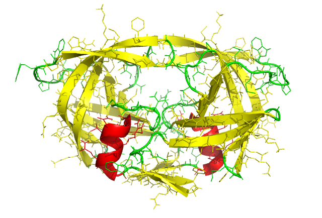
(a) Cartoon

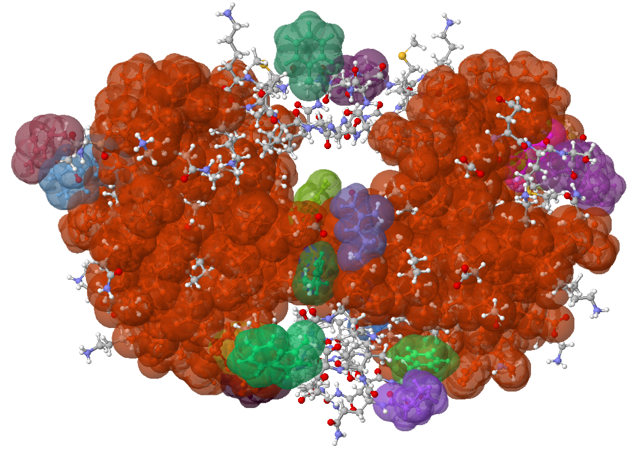
(b) Rigidity Analysis

Figure 1: Rigidity analysis (PDB 1HVR) identifies rigid clusters. Orange is the largest cluster with 1,371 atoms.

3.1.1 Mutants, Rigidity Distance

To generate in silico mutant structures corresponding to the mutation data in ProTherm, we used our ProMuteHT [2] software. In this study, we rely on the rigidity analysis results of the wild type (non-mutated protein), and a mutant, to assess the effects of a mutation. In our previous work [1, 6], we used an $RD_{WT\rightarrow mutant}$ rigidity distance metric to quantitatively assess the impact of mutating a residue to one of the other 19 naturally occurring amino acids:

$RD_{WT\rightarrow mutant}:\sum_{i=1}^{i=LRC}i\times[WT_{i}-Mut_{i}]$

where $WT$ refers to Wild Type, $Mut$ refers to mutant, and $LRC$ is the size of the Largest Rigid Cluster (in atoms). Each term of the summation $RD_{WT\rightarrow mutant}$ metric calculates the difference in the count of a specific cluster size, $i$, of the wild type and mutant, and weighs that difference by $i$.

3.2 Wet Lab Mutation Data – $\Delta\Delta G$

Labels ($\Delta\Delta G$) and metadata (pH, temperature, etc.) of mutations were retrieved from the ProTherm [15] database of mutation experiments. The rigidity features for each mutant and wild type were generated by rigidity analysis using the KINARI software. A total of $2,072$ data points from ProTherm meet the criteria for our experimental setup (i.e., single chain proteins, single mutations, any value of $\Delta\Delta G$). The input to our model is shown in Figure 2. The data set of 2,072 proteins is split into a training set of 1,438 proteins for fitting a classifier, a development set of 324 proteins for finding the best neural network configuration, and a test set of 310 proteins to test generalization error.

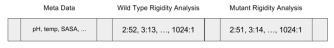
Figure 2: The form of a feature vector as input to the DNN. It consists of experiment meta data, such as Solvent Accessible Surface Area (SASA), pH, and temperature, concatenated with the rigid cluster frequencies of both wild type and mutant proteins.

3.3 Deep Neural Network Classifier

A deep neural network (DNN) classifier is a parameterized function mapping a real valued vector to a probability distribution over a set of classes. We model the probability distribution over classes of mutation as stabilizing, destabilizing, or inconclusive, as a function of the rigidity analyses and experimental conditions, using a DNN with $L$ hidden layers, $\textbf{h}_{(1)},\textbf{h}_{(2)},\dots,\textbf{h}_{(L)}$. This neural network classifier takes as input a feature vector ${\bf x}$ (Fig. 2) which we alternatively denote as as ${\bf h}_{(0)}$. The classifier outputs a probability vector ${\bf p}\in\mathbb{R}^{3}$, the elements of which are calculated as:

$$\textbf{p}_{k} = \frac{\texttt{exp}({{\bf o}_{k}})}{\sum_{j=1}^{3}\texttt{exp}({{\bf o}_{j}})}\mbox{, where}$$ (1)

$${\bf o} = {\bf U}{\bf h}_{(L)}+{\bf a}\mbox{ and }$$ (2)

$${\bf h}_{(\ell)} = f({\bf W}_{(\ell)}{\bf h}_{(\ell-1)}+{\bf b}_{(\ell)}).$$ (3)

where hidden activation function $f$ is one of three non-linear functions operating elementwise on matrices; the hyperbolic tangent function ($\tanh$), the logistic sigmoid function, or the rectified linear unit function (ReLU). The trainable parameters are the $L$ hidden weight matrices ($\bf{W}$), $L$ bias vectors ($\bf{b}$), and the output layer weights and bias $\bf{U}$ and $\bf{a}$.

All model parameters were trained with the Adam optimization algorithm [13], a variant of stochastic gradient descent. The training loss is the cross-entropy between the true distribution as determined by inconclusive bounds and the DNN’s predicted distribution.

The DNN hyper-parameters are model choices which cannot be learned via the training data through gradient descent. They are instead selected by evaluating models on the held out development set which is distinct from the training data and the testing set. The model choices we select in this fashion are the number of hidden layers, the size of each hidden layer (dimensions of the weight matrices W), the hidden activation function, and finally, the mini-batch size and learning rate used in stochastic gradient descent optimization.

We developed and trained our model architecture using the Tensorflow [5] Python library. Due to the small data set and GPU acceleration for computation, it takes under a minute to train a typical model.

3.4 Class Labels

As already mentioned, the $\Delta\Delta G$ values in ProTherm – especially those near zero – must be used with caution. To help determine which range of $\Delta\Delta G$ values should delimit stabilizing, destabilizing, and inconclusive mutations, we employed a principled approach by training models across a systematic set of different inconclusive ranges to train the best predictive model.

Class labels are represented as probability distributions over the three classes, i.e. real valued vectors in $\mathbb{R}^{3}$ that contain non-negative values and sum to one. A label for $\Delta\Delta G$ classification has one element as 1 and the other elements are zero. So, $[1\;\;0\;\;0]^{T}$ corresponds to a $\Delta\Delta G$ score which is negative and outside the range of indeterminacy (a destabilizing mutation), $[0\;\;1\;\;0]^{T}$ corresponds to an inconclusive $\Delta\Delta G$ score inside the range of indeterminacy, and $[0\;\;0\;\;1]^{T}$ corresponds to a $\Delta\Delta G$ score which is positive and outside the range of indeterminacy (a stabilizing mutation). To make a prediction from our model’s predicted class distribution, ${\bf p}$, we pick the most probable index.

Our ultimate goal is to find a pair of $\Delta\Delta G$ values for which a model can be trained to correctly predict the true labels that those cutoffs would create. For example if the $\Delta\Delta G$ value of an experiment is reported to be -0.8, and our model’s $\Delta\Delta G$ cutoffs were -0.6 and 0.7, the true label for that mutation would be destabilizing and a correct prediction from our model would also be destabilizing. For our best model, predictions should match true labels as closely as possible.

3.5 Experimental Setup

In order to assess our model’s effectiveness at classification for different inconclusive bounds, we trained 100 DNN models with random hyper-parameter configurations (the same configurations were used for all cutoff ranges). We normalized $\Delta\Delta G$ by dividing all values by 10, and executed a triangular grid search of cutoff ranges equivalent to -2.0 to 2.0, stepping by 0.1, in unnormalized $\Delta\Delta G$, for a total of 820 cutoff ranges. All 100 hyper-parameter configurations were assessed for each range, for a total of 8,200 configurations.

4 Confusion Matrices

For each of the 820 cutoff ranges, we identified the DNN model which achieved the best development set accuracy, and generated a confusion matrix for those model’s predictions on the held out test set. Confusion matrices are a method of visualizing the performance of the classification algorithm. They contain the same classes on the vertical and horizontal axis, with the vertical axis indicating true labels for each class and the horizontal axis indicating the model’s class predictions. Figure 3 is the confusion matrix generated by the classic heuristic for inconclusive $\Delta\Delta G$ of -0.5 to 0.5. The darker the color the more predictions fall into that intersection of true label and predicted label. A perfect classification model would have predictions only in the top left, center, and bottom right squares.

In addition to the standard metrics of a model’s accuracy in predicting the correct class, the confusion matrices offer insights in cases when a model is mis-classified. They allow us to assess Type I and Type II errors, false positive and false negative classifications, and also permit seeing how those incorrect classifications are being classified. This additional information enables assessing whether a particular mis-classification is more detrimental than another. For instance it may be better if a model is less accurate overall, but predicts very few unstable mutations as stabilizing and vice versa, but has a slightly higher than ideal tendency to label mutations as inconclusive.

		Hyper-parameters								Range				Metrics
Model		mb	lr	hs	nl	ha				L	U			loss	acc	macc	ratio
Figure 3		64	0.01	689	1	sigmoid				0.5	0.5			0.96	0.54	0.36	1.51
Figure 4		64	0.01	63	1	sigmoid				-2.00	-1.9			0.29	0.91	0.91	1.00
Figure 5		32	0.09	854	3	ReLU				-2.0	2.0			0.31	0.92	0.92	1.0
Figure 6		64	0.07	361	1	sigmoid				-0.5	0.7			1.15	0.61	0.48	1.28
Figure 7		128	0.01	604	1	sigmoid				-0.4	0.4			0.84	0.60	0.37	1.61

Table 2: Configuration and results for case study models. mb denotes minibatch size; lr denotes learning rate; hs denotes hidden layer size; nl denotes number of layers; ha denotes hidden activation function; L and U denote lower and upper cutoff ranges; loss denotes average test set cross-entropy between true and predicted values; acc denotes accuracy; macc denotes majority class accuracy; ratio is acc/macc.

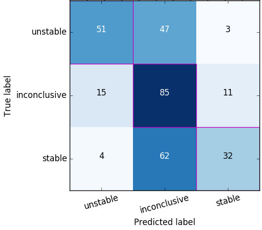
Figure 3: Test set confusion matrix for cutoffs -0.5, 0.5.

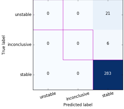
Figure 4: Test set confusion matrix for cutoffs -2.0, -1.9.

5 Results and Discussion

Table 2 reports hyper-parameters as well as several performance metrics for our models. The confusion matrices shown in Figures 3–6 further elucidate these models’ performances.

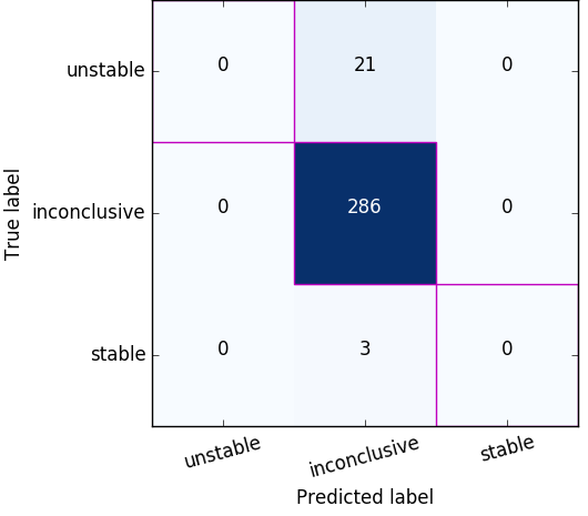
Figure 5: Test set confusion matrix with an unrealistic inconclusive range (-2.0,2.0) where most mutations are labeled as inconclusive.

We first note that when the vast majority of the $\Delta\Delta G$ values fall within a single region determined by the cutoff boundaries, a classification model can trivially achieve high accuracy by learning to predict the majority class. However, labels thus determined may be impractical for scientific pursuits. These situations are characterized by a high proportion of data points which fall into the majority class giving a high majority class accuracy (macc), which is indicated in Table 2. One such example is given in Figure 4 which has a small range of indeterminacy, $[-2,-1.9]$, with a large negative offset. For these bounds, $\texttt{macc}=91\%$, with only 6 inconclusive examples and 21 destabilizing examples. We can see from the confusion matrix that all examples were predicted as stabilizing mutations giving a 91% accuracy which amounts to a clearly unhelpful classifier. Another example of ill-conditioned labeling is shown in Figure 5. In this case the indeterminate range is ostensibly too large, $[-2,2]$ as the model has learned to classify most examples as inconclusive.

Figure 3 shows performance for ternary classification using the traditional $\Delta\Delta G$ range for exclusion of examples, $[-0.5,0.5]$. If we exclude the somewhat innocuous mistakes of examples which are incorrectly classified as inconclusive, along with the examples labeled as inconclusive which would be excluded in the traditional approach in the first place, and attend only to egregious mis-classification of stabilizing as non-stabilizing and vice-versa we achieve a 92.2% accuracy. From this method of preference, running counter to common practice, the optimal ranges for excluding $\Delta\Delta G$ are not necessarily centered on zero.

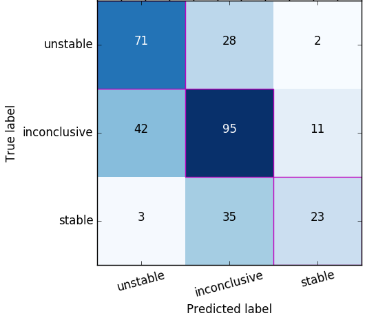
Figure 6: Test set confusion matrix for cutoffs -0.5 and 0.7, where false positive and false negative errors (top-right and bottom-left, respectively) are minimized.

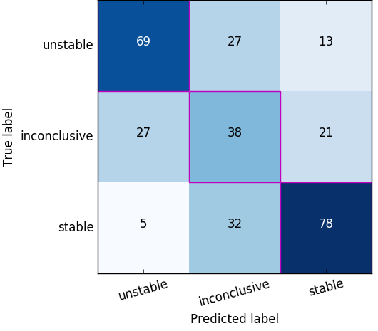
Figure 7: Test set confusion matrix for cutoffs -0.4 and 0.4, where the ratio of accuracy to majority class is maximized.

For instance, based on this criterion of binary predictions within the ternary classification schema, the best cutoff classification range from our experiments is shown in Figure 6 with an inconclusive range $[-0.5,0.7]$, giving a 94.4% accuracy for the binary subset classification task. On the same test set, for the ternary task, that model achieved an accuracy of 61%. Upon initial assessment this performance does not seem great on its own, but we are more concerned with the model’s classification of a destabilizing mutation as a stabilizing one, and vice versa, than we are of it mis-classifying an inconclusive mutation. In this case we see that for this cutoff range the model yields impressive mis-classification rates of 2% for destabilizing to stabilizing and 4% for stabilizing to destabilizing. Such low rates of mis-classification across the inconclusive zone help motivate these findings and suggest that this range is a potentially good $\Delta\Delta G$ cutoff set.

On the other hand, another promising criterion for optimal cutoff is be the ratio of accuracy (acc) to majority class accuracy, $\texttt{ratio}=\frac{\texttt{acc}}{\texttt{macc}}$, also displayed in Table 2. For any acceptable model this value should be greater than 1, with larger values being better. Figure 7 shows performance for a model with inconclusive range $[-0.4,0.4]$ and a significantly higher ratio value than the traditional cutoff

6 Conclusion and Future Work

As an extension on our prior work we were interested in assessing the potential of a deep neural network for classifying the effects of mutations. We performed a systematic search of the $\Delta\Delta G$ classification cutoff ranges in order to assess the potential viability of a deep neural network ternary classification approach to predicting of mutation affects. Rather than simply accept the general heuristic for classification boundaries of stabilizing, destabilizing or inconclusive, we strove for a more systematic approach. While our findings suggest that the heuristic of -0.5 to 0.5 is not a poor choice by any means, we proposed some compelling arguments for choosing other ranges as boundary conditions for $\Delta\Delta G$ values, namely it is most important to minimize false positive and false negative rates on the ternary task, and maximizing the ratio of accuracy to majority class accuracy are both more important metrics to consider besides accuracy.

For future work we plan to develop robust algorithmic approaches to assess the likely cutoff ranges in ML-based models. We are currently in the development of an end-to-end differentiable approach to jointly learn an optimal cutoff range alongside DNN parameters, as opposed to relying on a parameter sweep as in the current work. Also, expanding our data set with additional mutation $\Delta\Delta$G data – data for proteins with multiple mutations – will likely enhance the DNN’s learning and ultimately increase accuracy. We also hope to expand our study into other machine learning algorithms.

Acknowledgments

The authors would like to thank the Nvidia corporation for donating a Titan Xp GPU used in this research.

References

- [1] E. Andersson, R. Hsieh, H. Szeto, R. Farhoodi N. Haspel, and F. Jagodzinski. Assessing how multiple mutations affect protein stability using rigid cluster size distributions. In Proc ICCABS, pages 1–6, 2016.
- [2] E. Andersson and F. Jagodzinski. ProMuteHT : A high throughput compute pipeline for generating protein mutants in silico. In Proc. CSBW, 2017.
- [3] Emidio Capriotti, Piero Fariselli, and Rita Casadio. I-mutant2. 0: predicting stability changes upon mutation from the protein sequence or structure. Nucleic acids research, 33(suppl 2):W306–W310, 2005.
- [4] Chi-Wei Chen, Jerome Lin, and Yen-Wei Chu. iStable: off-the-shelf predictor integration for predicting protein stability changes. BMC bioinformatics, 14(2):S5, 2013.
- [5] Martín Abadi et al. TensorFlow: Large-scale machine learning on heterogeneous systems, 2015. Software available from tensorflow.org.
- [6] Roshanak Farhoodi, Max Shelbourne, Rebecca Hsieh, Nurit Haspel, Brian Hutchinson, and Filip Jagodzinski. Predicting the effect of point mutations on protein structural stability. In Proc. ACM-BCB, pages 247–252, 2017.
- [7] Maria E Figueroa, Omar Abdel-Wahab, Chao Lu, Patrick S Ward, Jay Patel, Alan Shih, Yushan Li, Neha Bhagwat, Aparna Vasanthakumar, Hugo F Fernandez, et al. Leukemic IDH1 and IDH2 mutations result in a hypermethylation phenotype, disrupt TET2 function, and impair hematopoietic differentiation. Cancer cell, 18(6):553–567, 2010.
- [8] N. Fox, F. Jagodzinski, and I. Streinu. KINARI-Lib: a C++ library for pebble game rigidity analysis of mechanical models. In Minisymposium on Publicly Available Geometric/Topological Software, Chapel Hill, NC, USA, June 2012.
- [9] Jianglin He, Sunny Choe, Robert Walker, Paola Di Marzio, David O Morgan, and Nathaniel R Landau. Human immunodeficiency virus type 1 viral protein R (Vpr) arrests cells in the G2 phase of the cell cycle by inhibiting p34cdc2 activity. Journal of virology, 69(11):6705–6711, 1995.
- [10] D.J. Jacobs and B. Hendrickson. An algorithm for two-dimensional rigidity percolation: the pebble game. Journal of Computational Physics, 137:346–365, 1997.
- [11] D.J. Jacobs, A.J. Rader, M.F. Thorpe, and L.A. Kuhn. Protein flexibility predictions using graph theory. Proteins 44, pages 150–165, 2001.
- [12] Shuli Kang, Gang Chen, and Gengfu Xiao. Robust prediction of mutation-induced protein stability change by property encoding of amino acids. Protein Engineering, Design & Selection, 22(2):75–83, 2008.
- [13] Diederik Kingma and Jimmy Ba. Adam: A method for stochastic optimization. arXiv preprint arXiv:1412.6980, 2014.
- [14] Tanja Kortemme and David Baker. A simple physical model for binding energy hot spots in protein–protein complexes. PNAS, 99(22):14116–14121, 2002.
- [15] MD Shaji Kumar, K Abdulla Bava, M Michael Gromiha, Ponraj Prabakaran, Koji Kitajima, Hatsuho Uedaira, and Akinori Sarai. Protherm and pronit: thermodynamic databases for proteins and protein–nucleic acid interactions. Nucleic acids research, 34(suppl_1):D204–D206, 2006.
- [16] Graham R Serjeant and Beryl E Serjeant. Sickle cell disease, volume 3. Oxford university press New York, 1992.
- [17] Novel Swine-Origin Influenza A H1N1 Virus and Investigation Team. Emergence of a novel swine-origin influenza a (h1n1) virus in humans. New England Journal of Medicine, 2009(360):2605–2615, 2009.