Tight Piecewise Convex Relaxations for
Global Optimization of Optimal Power Flow

Abstract

Since the alternating current optimal power flow (ACOPF) problem was introduced in 1962, developing efficient solution algorithms for the problem has been an active field of research. In recent years, there has been increasing interest in convex relaxations-based solution approaches that are often tight in practice. Based on these approaches, we develop tight piecewise convex relaxations with convex-hull representations, an adaptive, multivariate partitioning algorithm with bound tightening that progressively improves these relaxations and, given sufficient time, converges to the globally optimal solution. We illustrate the strengths of our algorithm using benchmark ACOPF test cases from the literature. Computational results show that our novel algorithm reduces the best-known optimality gaps for some hard ACOPF cases.

I Introduction

The optimal power flow problem is one of the most fundamental optimization problems for the economic and reliable operation of electric power systems. The ACOPF is a cost minimization problem with equality and inequality constraints setting bus voltage, line flows and generator dispatch. It was first introduced in 1962 and has been formulated in various forms over years, e.g., the polar power-voltage formulation and the rectangular power-voltage formulation [1]. Since the introduction of the ACOPF problem [2], the development of efficient solution technique for the ACOPF has remained an active field of research. The main challenges associated with solving the ACOPF include: a) non-convex and nonlinear mathematical models of ac physics, b) large-scale power grids, and c) limited computation time available in real-time dispatch applications. A fast and robust algorithm for obtaining high-quality and lower-cost dispatch solutions could improve the operational performance of power systems and save billions of dollars per year [1].

Various solution algorithms, ranging from heuristic to convex relaxation, have been studied within literature [3, 4]. Without losing generality, the ACOPF literature can be roughly categorized into three main research directions: a) finding locally optimal solutions quickly, b) deriving strong, convex relaxations and c) proving global optimality. In the local search literature, local solvers based on primal-dual interior point methods or sequential linearization heuristics are used to find feasible solutions efficiently without any guarantees on solution quality. In the relaxation literature, recent work has focused on deriving convex relaxations that produce tight lower bounds. These include SDP-based methods [5], Quadratic relaxations (QC) [4] and Second-order-cone (SOC) relaxations [6]. The performances of these existing methods have been evaluated and tested on well established power system test cases (i.e., Matpower and NESTA Test Cases) [7]. Though the relaxation approaches have empirically yielded strong lower bounds, there remain examples where the lower bounds are weak (e.g., case5, nesta_case30_fsr_api, nesta_case118_ieee_api, etc.) [4]. Finally, there have been recent efforts focused on obtaining globally optimal solutions through SOC and SDP-based relaxations [6, 8] using standard spatial branch-&-bound (sBB) approaches. Here, we focus on closing the optimality gaps on remaining hard instances by improving the QC relaxations, improved branching strategies, and leveraging high quality locally optimal solutions.

The focus of this paper is a novel approach for globally optimizing the ACOPF. Our work is built on an adaptive multivariate partitioning algorithm (AMP) proposed in [9, 10]. The approach is based on a two-stage algorithm that uses sBB-like methods tailored to OPF problems. In the first stage, we apply sequential bound-tightening techniques to the voltage and phase-angle variables and obtain tightest possible bounds by solving a sequence of convex problems [11, 12]. The second stage adaptively partitions convex envelopes of the ACOPF into piecewise convex regions around best-known local feasible solutions. This approach exploits the observation that local solutions to standard benchmark instances are already very good. Our recent results on generic mixed-integer nonlinear programs suggest that refining variable domains adaptively around best-known feasible solutions can dramatically speed up the convergence to global optimum [10, 13].

This paper makes three key contributions to solving the ACOPF problem. The first contribution develops an efficient partitioning scheme for tightening relaxations. In multilinear relaxations, many approaches build uniform, piecewise relaxations via univariate or bivariate partitioning [14]. One drawback of such approaches is that a large number of partitions may be needed to attain global optimum. Thus, these approaches are often restricted to small problems. To address inefficiencies of these approaches, we develop an adaptive tightening algorithm with non-uniform partitions, where we selectively partition convex envelopes that heuristically appear to tighten the relaxations.

Our second contribution lies in applying well-known ideas for deriving the tightest possible convex relaxations (convex-hulls) for multilinear functions as they play a crucial role for developing efficient global optimization approaches. Multilinears (up to trilinear) appear in the polar form of the ACOPF, for which there has been a recent development in developing strong convex quadratic relaxations (QC) [15, 4]. However, these relaxations employ recursive McCormick envelopes to handle the trilinear terms, which rarely capture their convex hulls. In the optimization literature, specifically for a trilinear function, [16] (Meyer-Floudas envelopes) describes the convex hull by deriving all it’s facets, and for a generic multilinear function, convex hull is typically formulated as a convex combination of the extreme points of the function [17]. Owing to the simplicity of the latter idea from the global optimization perspective, we further strengthen the QC relaxations to obtain tighter lower bounds for the OPF problem. Also, we develop tight piecewise convex relaxations of the convex-hull representation for trilinear and quadratic functions by extending the ideas of approximating univariate/bivariate functions [18, 19]. To the best of our knowledge, this is the first paper which applies tight representations of piecewise convex relaxations for ACOPF.

The third contribution of this paper is a novel algorithm that combines iterative partitioning (using piecewise relaxations) with bound tightening to globally solve the ACOPF (given sufficient time). This algorithm first applies “optimality-based bound tightening” by solving a sequence of min. and max. problems on voltage and phase angle difference variables [20, 11, 12]. Second, the algorithm iteratively partitions the convex envelopes to tighten the lower bound. Simultaneously, the algorithm updates locally feasible solutions based to tighten the upper bound. The combination of tightening the upper and lower bound yields an algorithm akin to sBB that determines the globally optimal solution.

This paper is organized as follows: In section II, we first revisit the ACOPF problem and the improved QC relaxation with convex hull representation. Then, we introduce piecewise relaxations in section IV. Section V discusses our global optimization algorithm. In section VI, we evaluate the proposed improvements on various hard test cases and conclude the paper in section VII.

II AC Optimal Power Flow Problem

Nomenclature
Sets and Parameters
$\cal{N}$ - set of nodes (buses)
$\cal{G}$ - set of generators
${\cal{G}}_{i}$ - set of generators at bus $i$
$\cal{E}$ - set of from edges (lines)
$\cal{E}^{R}$ - set of to edges (lines)
$\boldsymbol{c}_{0},\boldsymbol{c}_{1},\boldsymbol{c}_{2}$ - generation cost coefficients
$\boldsymbol{i}$ - imaginary number constant
$\boldsymbol{Y}_{ij}=\boldsymbol{g}_{ij}+\boldsymbol{i}\boldsymbol{b}_{ij}$ - admittance on line $ij$
$\boldsymbol{S}_{i}^{\boldsymbol{d}}=\boldsymbol{p}_{i}^{\boldsymbol{d}}+\boldsymbol{i}\boldsymbol{q}_{i}^{\boldsymbol{d}}$ - AC power demand at bus $i$
$\overline{\boldsymbol{S}}_{ij}$ - apparent power limit on line $ij$
$\underline{\boldsymbol{\theta}}_{ij},\overline{\boldsymbol{\theta}}_{ij}$ - phase angle difference limits on line $ij$
$\boldsymbol{\theta}_{ij}^{\boldsymbol{M}}$ - $\max(\mid\underline{\boldsymbol{\theta}}_{ij}\mid,\mid\overline{\boldsymbol{\theta}}_{ij}\mid)$ on line ij
$\underline{\boldsymbol{v}}_{i},\overline{\boldsymbol{v}}_{i}$ - voltage magnitude limit at bus $i$
$\underline{\boldsymbol{S}}_{i}^{\boldsymbol{g}}$, $\overline{\boldsymbol{S}}_{i}^{\boldsymbol{g}}$ - power generation limit at bus $i$
$\mathfrak{R}(\cdot)$ - real part of a complex number
$\mathfrak{T}(\cdot)$ - imaginary part of a complex number
$(\cdot)^{*}$ - hermitian conjugate of a complex number
$\mid\cdot\mid,\angle\cdot$ - magnitude, angle of a complex number

Continuous variables
${V_{i}}=v_{i}\boldsymbol{e}^{\boldsymbol{i}\theta_{i}}$ - AC voltage at bus $i$
$\theta_{ij}=\angle V_{i}-\angle V_{j}$ - phase angle difference on line $ij$
$W_{ij}$ - AC voltage product on line $ij$, i.e., $V_{i}V^{*}_{j}$
$S_{ij}=p_{ij}+\boldsymbol{i}q_{ij}$ - AC power flow on line $ij$
$S^{g}_{i}=p^{g}_{i}+\boldsymbol{i}q^{g}_{i}$ - AC power generation at bus $i$
$l_{ij}$ - current magnitude squared on line $ij$

In this paper, constants are typeset in bold face. In the AC power flow equations, the primitives, $V_{i}$, $S_{ij}$, $S^{g}_{i}$, $\boldsymbol{S}_{i}^{\boldsymbol{d}}$ and $\boldsymbol{Y}_{ij}$ are complex quantities. Given any two complex numbers (variables/constants) $z_{1}$ and $z_{2}$, $z_{1}\geqslant z_{2}$ implies $\mathfrak{R}({z}_{1})\geqslant\mathfrak{R}({z}_{2})$ and $\mathfrak{T}({z}_{1})\geqslant\mathfrak{T}({z}_{2})$. $|\cdot|$ represents absolute value when applied on a real number. Statement $A\wedge B$ is true iff $A$ and $B$ are both true; else it is false. $\langle f(\cdot)\rangle^{R}$ represents the constraints corresponding to the convex relaxation of function $f(\cdot)$.

This section describes the mathematical formulation of the ACOPF problem using the polar formulation. Here, a power network is represented as a graph, $(\cal{N},\cal{E})$, where $\cal{N}$ and $\cal{E}$ are the buses and transmission lines, respectively. Generators are connected to buses where ${\cal{G}}_{i}$ are the generators at bus $i$. We assume that there is power demand (load) at every bus, some of which is zero. The optimal solution to the ACOPF problem minimizes generation costs for a specified demand and satisfies engineering constraints and power flow physics. More formally, the ACOPF problem is mathematically stated as:

$$\boldsymbol{\cal{P}}:=\min\sum_{i\in\cal{G}}\boldsymbol{c}_{2i}(\mathfrak{R}(S_{i}^{g})^{2})+\boldsymbol{c}_{1i}\mathfrak{R}(S_{i}^{g})+\boldsymbol{c}_{0i}$$ (1a)

$$\textit{s.t.}\ \ \sum_{k\in{\cal{G}}_{i}}S_{k}^{g}-\boldsymbol{S}_{i}^{\boldsymbol{d}}=\sum_{(i,j)\in\cal{E}\cup\cal{E^{R}}}S_{ij}\ \ \hskip 15.0pt\forall i\in\cal{N}$$ (1b)

$$\qquad S_{ij}=\boldsymbol{Y}^{*}_{ij}W_{ii}-\boldsymbol{Y}^{*}_{ij}W_{ij}\hskip 15.0pt\forall(i,j)\in\cal{E}$$ (1c)

$$\qquad S_{ji}=\boldsymbol{Y}^{*}_{ij}W_{jj}-\boldsymbol{Y}^{*}_{ij}W^{*}_{ij}\hskip 15.0pt\forall(i,j)\in\cal{E}$$ (1d)

$$\qquad W_{ii}=|V_{i}|^{2}\ \ \forall i\in\cal{N}$$ (1e)

$$\qquad W_{ij}=V_{i}V_{j}^{*}\ \ \forall(i,j)\in\cal{E}$$ (1f)

$$\qquad\underline{\boldsymbol{\theta}}_{ij}\leqslant\angle V_{i}-\angle V_{j}\leqslant\overline{\boldsymbol{\theta}}_{ij}\ \ \forall(i,j)\in\cal{E}$$ (1g)

$$\qquad\underline{\boldsymbol{v}}_{i}\leqslant|V_{i}|\leqslant\overline{\boldsymbol{v}}_{i}\ \ \forall i\in\cal{N}$$ (1h)

$$\qquad\underline{\boldsymbol{S}}_{i}^{\boldsymbol{g}}\leqslant S^{g}_{i}\leqslant\overline{\boldsymbol{S}}_{i}^{\boldsymbol{g}}\ \ \forall i\in\cal{G}$$ (1i)

$$\qquad|S_{ij}|\leqslant\overline{\boldsymbol{S}}_{ij}\ \ \forall(i,j)\in\cal{E}\cup\cal{E^{R}}$$ (1j)

In formulation (1), the convex quadratic objective (1a) minimizes total generator dispatch cost. Constraint (1b) corresponds to the nodal power balance at each bus, e.g. Kirchoff’s current law. Constraints (1c) through (1f) model the AC power flow on each line in complex number notation. Constraint (1g) limits the phase angle difference on each line. Constraint (1h) limits the voltage magnitude at each bus. Constraint (1i) restricts the apparent power output of each generator. Finally, constraint (1j) restricts the total electric power transmitted on each line. For simplicity, we omit the details of constant bus shunt injections, transformer taps, phase shifts, and line charging, though we include them in the computational studies.

The ACOPF is a hard, nonconvex problem [21] where the source of nonconvexity is in constraints (1e) and (1f), which reduce to:

$$W_{ii} =v_{i}^{2}$$ (2a)

$$\mathfrak{R}(W_{ij}) =v_{i}v_{j}\cos(\theta_{ij})$$ (2b)

$$\mathfrak{T}(W_{ij}) =v_{i}v_{j}\sin(\theta_{ij})$$ (2c)

To address the nonconvexities, we first summarize a state-of-the-art convex relaxation with some enhancements and then derive tighter piecewise relaxations.

III Convex Quadratic Relaxation of the ACOPF

In this section, we discuss the features of the convex quadratic (QC) relaxation of the ACOPF [11, 4]. Though there are numerous other relaxations in the literature, we adopt the QC relaxations as it has been observed to be empirically tight, computationally stable, and efficient. We further tighten the sinusoidal relaxations of [11, 4] for certain conditions and introduce the tightest possible convex relaxations for trilinear functions.

Quadratic function relaxation
Given a voltage variable, $v_{i}\in[\underline{\bf v}_{i},\overline{\bf v}_{i}]$, the tightest convex envelop is formulated with a lifted variable, $\widehat{w}_{i}\in\langle v_{i}^{2}\rangle^{R}$, where

$$\widehat{w}_{i}\geqslant v_{i}^{2}$$ (3a)

$$\widehat{w}_{i}\leqslant(\boldsymbol{\underline{v}}_{i}+\boldsymbol{\overline{v}}_{i})v_{i}-\boldsymbol{\underline{v}}_{i}\boldsymbol{\overline{v}}_{i}$$ (3b)

Cosine function relaxation
Under the assumptions that $|\underline{\boldsymbol{\theta}}_{ij}|$ is not always equal to $|\overline{\boldsymbol{\theta}}_{ij}|$ and $\boldsymbol{\theta}_{ij}^{\boldsymbol{M}}\leqslant\pi/2$, the convex quadratic envelope of the cosine function is formulated with a lifted variable $\widehat{cs}_{ij}\in\langle\cos(\theta_{ij})\rangle^{R}$ where

$$\widehat{cs}_{ij}\leqslant 1-\frac{1-\cos(\boldsymbol{\theta}_{ij}^{\boldsymbol{M}})}{(\boldsymbol{\theta}_{ij}^{\boldsymbol{M}})^{2}}(\theta_{ij}^{2})$$ (4a)

$$\widehat{cs}_{ij}\geqslant\frac{\cos(\overline{\boldsymbol{\theta}}_{ij})-\cos(\underline{\boldsymbol{\theta}}_{ij})}{\overline{\boldsymbol{\theta}}_{ij}-\underline{\boldsymbol{\theta}}_{ij}}(\theta_{ij}-\overline{\boldsymbol{\theta}}_{ij})+\cos(\underline{\boldsymbol{\theta}}_{ij})$$ (4b)

Sine function relaxation
First, let the first-order Taylor’s approximation of $\sin(\theta)$ at $\overline{\boldsymbol{\theta}}$ be

$$f^{oa}(\overline{\boldsymbol{\theta}})=\sin(\overline{\boldsymbol{\theta}})+\cos(\overline{\boldsymbol{\theta}})(\theta-\overline{\boldsymbol{\theta}}).$$

Second, let the secant function between $(\overline{\boldsymbol{\theta}},\sin(\overline{\boldsymbol{\theta}}))$ and $(\underline{\boldsymbol{\theta}},\sin(\underline{\boldsymbol{\theta}}))$ be

$$f^{sec}(\underline{\boldsymbol{\theta}},\overline{\boldsymbol{\theta}})=\frac{\sin(\overline{\boldsymbol{\theta}})-\sin(\underline{\boldsymbol{\theta}})}{\overline{\boldsymbol{\theta}}-\underline{\boldsymbol{\theta}}}(\theta-\underline{\boldsymbol{\theta}})+\sin(\underline{\boldsymbol{\theta}}).$$

Finally, given bounds $[\underline{\boldsymbol{\theta}},\overline{\boldsymbol{\theta}}]$, we use $\boldsymbol{\theta}^{\boldsymbol{\mu}}=\frac{(\boldsymbol{\underline{\theta}}+\boldsymbol{\overline{\theta}})}{2}$ to denote the midpoint of the bounds.

Since the bounds on phase-angle differences can be non-symmetric, we derive convex relaxations of the sine function for three cases:
Case (a): When $(\underline{\boldsymbol{\theta}}_{ij}<0)\wedge(\overline{\boldsymbol{\theta}}_{ij}>0)$, the polyhedral relaxation, as described in [4], is characterized with lifted variable $\widehat{sn}_{ij}\in\langle\sin(\theta_{ij})\rangle^{R}$ where

$$\widehat{sn}_{ij}\leqslant f^{oa}(\boldsymbol{\theta}_{ij}^{\boldsymbol{M}}/2),\ \ \widehat{sn}_{ij}\geqslant f^{oa}(-\boldsymbol{\theta}_{ij}^{\boldsymbol{M}}/2)$$ (5)

Case (b): When $(\underline{\boldsymbol{\theta}}_{ij}<0)\wedge(\overline{\boldsymbol{\theta}}_{ij}<0)$, we derive a tighter polyhedral relaxations that exploits a lack of an inflection point in the sine function. This relaxation is defined by:

$$\widehat{sn}_{ij}\leqslant f^{sec}(\underline{\boldsymbol{\theta}}_{ij},\overline{\boldsymbol{\theta}}_{ij}),$$ (6a)

$$\widehat{sn}_{ij}\geqslant f^{oa}(\boldsymbol{\theta}_{ij})\ \ \forall\boldsymbol{\theta}_{ij}\in\{\underline{\boldsymbol{\theta}}_{ij},\boldsymbol{\theta}_{ij}^{\boldsymbol{\mu}},\overline{\boldsymbol{\theta}}_{ij}\}.$$ (6b)

Case (c): Like case (b), when $(\underline{\boldsymbol{\theta}}_{ij}>0)\wedge(\overline{\boldsymbol{\theta}}_{ij}>0)$, a tighter polyhedral relaxation for the sine function is:

$$\widehat{sn}_{ij}\geqslant f^{sec}(\underline{\boldsymbol{\theta}}_{ij},\overline{\boldsymbol{\theta}}_{ij}),$$ (7a)

$$\widehat{sn}_{ij}\leqslant f^{oa}(\boldsymbol{\theta}_{ij})\ \ \forall\boldsymbol{\theta}_{ij}\in\{\underline{\boldsymbol{\theta}}_{ij},\boldsymbol{\theta}_{ij}^{\boldsymbol{\mu}},\overline{\boldsymbol{\theta}}_{ij}\}.$$ (7b)

A geometric visualization of the relaxations of the sine function for cases (a) and (c) are shown in Figure 1.

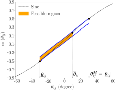
(a) Case (a)

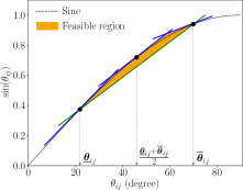
(b) Case (c)

Figure 1: Polyhedral relaxations for sinusoidal function

Trilinear function relaxation
After introducing the lifted variables, $\widehat{cs}_{ij}$ and $\widehat{sn}_{ij}$ from above, the non-convex constraints in (2b) and (2c) become trilinear functions of the form $v_{i}v_{j}\widehat{cs}_{ij}$ and $v_{i}v_{j}\widehat{sn}_{ij}$. In the literature, bilinear McCormick relaxations are applied recursively to relax these trilinear functions [3, 4], which rarely capture their convex hull. Instead, we relax the trilinear function based on the convex hull of the extreme points using techniques from [17].

Given a trilinear function $\phi(x_{1},x_{2},x_{3})=x_{1}x_{2}x_{3}$ with respective variable bounds $[\boldsymbol{\underline{x}_{1}},\boldsymbol{\overline{x}_{1}}],[\boldsymbol{\underline{x}_{2}},\boldsymbol{\overline{x}_{2}}],[\boldsymbol{\underline{x}_{3}},\boldsymbol{\overline{x}_{3}}]$, the extreme points of $\phi(\cdot)$ are given by the Cartesian product $(\underline{\boldsymbol{x}}_{1},\overline{\boldsymbol{x}}_{1})\times(\underline{\boldsymbol{x}}_{2},\overline{\boldsymbol{x}}_{2})\times(\underline{\boldsymbol{x}}_{3},\overline{\boldsymbol{x}}_{3})=\langle\boldsymbol{\xi_{1}},\boldsymbol{\xi_{2}},\ldots,\boldsymbol{\xi_{8}}\rangle$. We use $\boldsymbol{\xi}^{i}_{\boldsymbol{k}}$ to denote the coordinate of $x_{i}$ in $\boldsymbol{\xi_{k}}$. The convex hull of the extreme points of $x_{1}x_{2}x_{3}$ is then given by

$$\sum_{k=1..8}\lambda_{k}=1,\quad\lambda_{k}\geqslant 0,\quad\forall k=1,\ldots,8,$$ (8a)

$$\widehat{x}=\sum_{k=1..8}\lambda_{k}\phi(\boldsymbol{\xi_{k}}),\quad x_{i}=\sum_{k=1..8}\lambda_{k}\boldsymbol{\xi}^{i}_{\boldsymbol{k}}$$ (8b)

The notation $\langle x_{1},x_{2},x_{3}\rangle^{\lambda}$ is used to denote the $\lambda$-based relaxation of a trilinear function as defined above. Thus, the relaxation of $x_{1}x_{2}x_{3}$ is stated as $\widehat{x}=\langle x_{1},x_{2},x_{3}\rangle^{\lambda}$. We note that this formulation generalizes to any multilinear function and is equivalent to the standard McCormick relaxation for bilinear functions.

Current-magnitude constraints
We also add the second-order conic constraints that connect apparent power flow on lines, ($S_{ij}$), with current magnitude squared variables, ($l_{ij}$) [15, 4]. The complete convex quadratic formulation with tightest trilinear relaxation of the ACOPF is then stated as:

$$\boldsymbol{\mathcal{P}^{QC}}:=\min\sum_{i\in\cal{G}}\boldsymbol{c}_{2i}(\mathfrak{R}(S_{i}^{g})^{2})+\boldsymbol{c}_{1i}\mathfrak{R}(S_{i}^{g})+\boldsymbol{c}_{0i}$$ (9a)

$$\textit{s.t.}\ \ \mathrm{Constraints}\ \eqref{s_balance}-\eqref{sji},$$ (9b)

$$\qquad\mathrm{Constraints}\ \eqref{theta}-\eqref{s_cap},$$ (9c)

$$\qquad W_{ii}=\widehat{w}_{i},\ \widehat{w}_{i}\in\langle v_{i}^{2}\rangle^{R}\ \ \forall i\in\cal{N}$$ (9d)

$$\qquad\mathfrak{R}(W_{ij})=\widehat{wcs}_{ij},\ \mathfrak{T}(W_{ij})=\widehat{wsn}_{ij},\ \ \forall(i,j)\in\cal{E}$$ (9e)

$$\qquad\widehat{wcs}_{ij}\in\langle v_{i}v_{j}\widehat{cs}_{ij}\rangle^{\lambda},\ \widehat{wsn}_{ij}\in\langle v_{i}v_{j}\widehat{sn}_{ij}\rangle^{\lambda},$$ (9f)

$$\qquad\widehat{cs}_{ij}\in\langle\cos(\theta_{ij})\rangle^{R},\ \widehat{sn}_{ij}\in\langle\sin(\theta_{ij})\rangle^{R},$$ (9g)

$$\qquad S_{ij}+S_{ji}=Z_{ij}l_{ij}\ \ \forall(i,j)\in\cal{E}$$ (9h)

$$\qquad|S_{ij}|^{2}\leqslant W_{ii}l_{ij}\ \ \forall(i,j)\in\cal{E}.$$ (9i)

IV Piecewise Convex Relaxations

One of the weaknesses of the convex quadratic relaxations described in section III is that the relaxation is not tight when the bounds of the variables are wide. To address this issue, recent work [11, 12] has developed approaches to tighten variable bounds, sometimes significantly. However, there are still a few OPF instances with large optimality gaps. In this section, we focus on developing tighter piecewise convex relaxations for quadratic and trilinear functions. To the best of our knowledge, this is the first paper that considers global optimization of ACOPF via piecewise polyhedral relaxations.

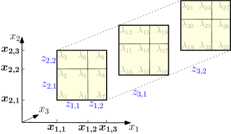
Figure 2: Partitioned variable domains for a trilinear function. Blue font indicates binary variables.

Piecewise trilinear functions
The basis for our piecewise relaxation is the piecewise linear approximation of continuous (mostly bivariate) separable functions that are solved with mixed integer programs (the $\lambda$-method) [18, 22, 19]. Based on these approaches, we tighten the trilinear function relaxations of $v_{i}v_{j}\widehat{cs}_{ij}$ and $v_{i}v_{j}\widehat{sn}_{ij}$ with a $\lambda$ formulation for modeling piecewise unions of polyhedrons.

The piecewise relaxation partitions the variable domains by introducing discretization points within the variable bounds. Binary variables are used to control the selection of a partition and its associated local convex hull relaxation (in (8)) of the trilinear function. As the number of partitions approaches $\infty$, the partitioning exactly represents the original trilinear function. Without loss of generality and for ease of exposition, we restrict the discussion of piecewise polyhedral relaxations for trilinear functions with two partitions on every variable.

Notation: Let the discretization points of variable $x_{i}$ be $(\boldsymbol{\underline{x}_{i}}=\boldsymbol{x_{i,1}})\leqslant\boldsymbol{x_{i,2}}\leqslant(\boldsymbol{x_{i,3}}=\boldsymbol{\overline{x}_{i}})$. Also, let $z_{i,1}\in\{0,1\}$ and $z_{i,2}\in\{0,1\}$ be the binary partition variables of $x_{i}$. We define $\mathcal{K}=\{1,..,27\}$ as the set of the first 27 positive integers. For $k\in\mathcal{K}$, $\boldsymbol{\xi}_{k}$ is used to denote the coordinates of the $k$th extreme point. For every extreme point, $\boldsymbol{\xi}_{k}$, there is a nonnegative mulitiplier variable $\lambda_{k}$. The partitioned domains of the trilinear function are graphically illustrated in Fig. 2. Using this notations, we now present SOS-II-type constraints that model the piecewise union of polyhedrons of a trilinear function:

$$\widehat{x}=\sum_{k\in\mathcal{K}}\lambda_{k}\phi(\boldsymbol{\xi}_{k}),\quad x_{i}=\sum_{k\in\mathcal{K}}\lambda_{k}\boldsymbol{\xi}_{k}^{i},$$ (10a)

$$\sum_{k\in\mathcal{K}}\lambda_{k}=1,\quad\lambda_{k}\geqslant 0,\ \forall k\in\mathcal{K},$$ (10b)

$$z_{i,1},z_{i,2}\in\{0,1\},\quad z_{i,1}+z_{i,2}=1,\ \forall i=1,..,3,$$ (10c)

$$z_{1,1}\geqslant\sum_{k\in\widetilde{\mathcal{K}}}\lambda_{k},\ \widetilde{\mathcal{K}}=\{1,2,3,10,11,12,19,20,21\},$$ (10d)

$$z_{1,2}\geqslant\sum_{k\in\widetilde{\mathcal{K}}}\lambda_{k},\ \widetilde{\mathcal{K}}=\{7,8,9,16,17,18,25,26,27\},$$ (10e)

$$z_{2,1}\geqslant\sum_{k\in\widetilde{\mathcal{K}}}\lambda_{k},\ \widetilde{\mathcal{K}}=\{1,4,7,10,13,16,9,22,25\},$$ (10f)

$$z_{2,2}\geqslant\sum_{k\in\widetilde{\mathcal{K}}}\lambda_{k},\ \widetilde{\mathcal{K}}=\{3,6,9,12,15,18,21,24,27\},$$ (10g)

$$z_{1,1}+z_{1,2}\geqslant\sum_{k\in\widetilde{\mathcal{K}}}\lambda_{k},\ \widetilde{\mathcal{K}}=\{4,5,6,13,14,15,22,23,24\},$$ (10h)

$$z_{2,1}+z_{2,2}\geqslant\sum_{k\in\widetilde{\mathcal{K}}}\lambda_{k},\ \widetilde{\mathcal{K}}=\{2,5,8,11,14,17,20,23,26\},$$ (10i)

$$z_{3,1}\geqslant\sum_{k=1}^{9}\lambda_{k},\quad z_{3,1}+z_{3,2}\geqslant\sum_{k=10}^{18}\lambda_{k},\quad z_{3,2}\geqslant\sum_{k=19}^{27}\lambda_{k}.$$ (10j)

Constraints (10a)-(10c) model the convex combination of extreme points and disjunctions. They force one partition for each variable to be active. Constraints (10d)-(10j) enforce the adjacency conditions for the $\lambda$ variables. These resemble SOS-II constraints. The formulation in (10) has many interesting polyhedral properties. For example, the projection of this polytope on to the space of $\{x_{1},x_{2},x_{3},\widehat{x}\}$ has integral extreme points. This is one of the primary reasons this formulation can be computationally efficient For further theoretical details, we delegate the reader to [22, 19].

Piecewise quadratic functions

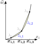
Figure 3: Piecewise quadratic regions. Blue font indicates binary variables.

Using the same notation, the SOS-II constraints of piecewise quadratic constraints are modeled using a piecewise union of convex quadratic regions (Fig. 3). To the best of our knowledge, this is the first time the piecewise quadratic regions of the voltage squared variables have been modeling using the $\lambda$ formulation.

$$\widehat{w}_{i}\geqslant x_{i}^{2},\quad\widehat{w}_{i}\leqslant\sum_{k=1,2,3}\lambda_{k}\boldsymbol{x_{i}}^{2}_{k},\quad x_{i}=\sum_{k=1,2,3}\lambda_{k}\boldsymbol{x_{i}}_{k},$$ (11a)

$$\sum_{k=1,2,3}\lambda_{k}=1,\quad\lambda_{k}\geqslant 0,\ \forall k=1,2,3,$$ (11b)

$$z_{i,1},z_{i,2}\in\{0,1\},\quad z_{i,1}+z_{i,2}=1,$$ (11c)

$$z_{i,1}\geqslant\lambda_{1},\quad z_{i,2}\geqslant\lambda_{3},\quad z_{i,1}+z_{i,2}\geqslant\lambda_{2}.$$ (11d)

Strengthening valid inequalities
Though the formulations in (10) and (11) are necessary and sufficient to characterize the piecewise relaxations of trilinear and quadratic functions, we observed that the inclusion of the following (simple) valid constraints improved the computational performance of $\lambda$ formulations tremendously. For a given variable $x_{i}$ with two partitions (as described earlier), the constraint is as follows:

$$z_{i,1}\boldsymbol{x_{i,1}}+z_{i,2}\boldsymbol{x_{i,2}}\leqslant x_{i}\leqslant z_{i,1}\boldsymbol{x_{i,2}}+z_{i,2}\boldsymbol{x_{i,3}}$$ (12)

Finally, for a given trilinear or quadratic function with a finite number of partitions, we use $\langle\cdot\rangle^{\lambda_{p}}$ to denote the piecewise $\lambda$-formulation of (10) and (11), respectively. The complete piecewise convex relaxation of the ACOPF is then stated as:

$$\boldsymbol{\mathcal{P}^{QC^{\lambda}}}:=\min\sum_{i\in\cal{G}}\boldsymbol{c}_{2i}(\mathfrak{R}(S_{i}^{g})^{2})+\boldsymbol{c}_{1i}\mathfrak{R}(S_{i}^{g})+\boldsymbol{c}_{0i}$$ (13a)

$$\textit{s.t.}\ \ \mathrm{Constraints}\ \eqref{s_balance}-\eqref{sji},\ \eqref{theta}-\eqref{s_cap}$$ (13b)

$$\qquad\mathrm{Constraints}\ \eqref{eq:wcs_wsn},\ \eqref{loss}-\eqref{SOC}$$ (13c)

$$\qquad W_{ii}=\widehat{w}_{i},\ \widehat{w}_{i}\in\langle v_{i}^{2}\rangle^{\lambda_{p}}\ \ \forall i\in\cal{N}$$ (13d)

$$\qquad\widehat{wcs}_{ij}\in\langle v_{i}v_{j}\widehat{cs}_{ij}\rangle^{\lambda_{p}},\ \widehat{wsn}_{ij}\in\langle v_{i}v_{j}\widehat{sn}_{ij}\rangle^{\lambda_{p}}.$$ (13e)

V Global optimization of ACOPF

Adaptive Multivariate Partitioning
To globally solve the ACOPF problem, we use the Adaptive Multivariate Partitioning (AMP) algorithm described in [9, 10]. The key idea of AMP is that AMP leverages the observations that solutions based on relaxations to ACOPF are often tight in practice and that locally optimal solutions are also very good [4]. AMP iteratively introduces narrow partitions around these relaxations.

A high-level pseudo-code for AMP is given in Algorithm 1. In this algorithm, we use the notation $\sigma$ to denote a solution to the ACOPF, $f(\sigma)$ to denote the objective value of $\sigma$, and $\sigma(x)$ to denote the assignment of variable $x$ in $\sigma$. In Lines 2-3, a feasible solution, $\overline{\sigma}$, and a lower bound, $\underline{\sigma}$, are computed. Here, the lower bound is computed without partitioning any variables. In line 4, we sequentially tighten the bounds of the voltage magnitude, ${v_{i}}$, and phase angle differences, $\theta_{ij}$, using optimization-based bound tightening (BT) [11, 12]. The new bounds on $\theta_{ij}$ are used to tighten $\widehat{cs}_{ij}$ and $\widehat{sn}_{ij}$ using the cases defined in equations 4-7. We would like to note that, though the importance of BT has been already observed for ACOPF problems, the bounds we obtain in this paper are tighter than in [11, 12] since formulation (9) is based on the convex-hull representation of trilinear functions.

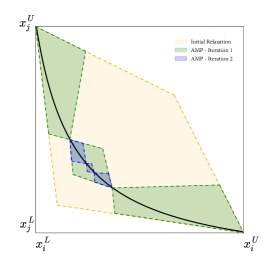
Figure 4: Example of variable partitioning in AMP for a bilinear function. Given an initial relaxation (tan region) and an initial feasible point (middle of the black curve), the function InitializePartitions creates a narrow partition around the feasible point (middle green region) and two wide partitions (outer green regions) around it. The size of the narrow partition is controlled by a user parameter, $\Delta$. The relaxation is iteratively tightened by the function TightenPartitions around relaxed solutions. This figure shows the partitioning of one iteration (blue regions).

Line 5 describes our variable selection strategy for partitioning (discussed later). This is the main point of departure (and contribution) from the AMP algorithm discussed in [10]. Line 6 initializes the piecewise partitions of variables in $\mathcal{X}$ around those variables’ assignments in $\overline{\sigma}$ (see Figure 4). Line 7 then updates the lower bound using the piecewise relaxation. Line 9 creates new partitions $\mathcal{X}$ around the updated lower bound (see Figure 4). Lines 10-13 then update the upper and lower bounds of the ACOPF. The upper bound (feasible solution) is updated by fixing the the ACOPF to the partition selected in $\underline{\sigma}$. and attempting to find a (better) feasible solution using a local solver. The process is repeated until the objective values of the upper and lower bound converge or a time-out criteria is met (Line 8). The full details of all these procedures are discussed in [10]. We note that this is the first time this algorithm has been applied to ACOPF represented in the polar form.

Algorithm 1 Adaptive Multivariate Partitioning (AMP)

1:function AMP

2:      $\overline{{\sigma}}\leftarrow$ Solve(${\mathcal{P}}$)

3:      $\underline{{\sigma}}\leftarrow$ Solve(${\mathcal{P}^{QC}}$)

4:      $\underline{\theta}_{ij},\overline{\theta}_{ij},\underline{v}_{i},\overline{v}_{i},\underline{\widehat{cs}}_{ij},\overline{\widehat{cs}}_{ij},\underline{\widehat{sn}}_{ij},\overline{\widehat{sn}}_{ij}\leftarrow$TightBounds(${\overline{{\sigma}}}$)

5:      $\mathcal{X}\leftarrow$SelectPartitionVariables($\overline{{\sigma}},\underline{{\sigma}}$)

6:      ${\mathcal{I}}\leftarrow$InitializePartitions($\mathcal{X},\mathcal{P},\overline{{\sigma}}$)

7:      $\underline{{\sigma}}\leftarrow$ Solve(${\mathcal{P}^{QC^{\lambda}}}$)

8:     while $\left(\frac{f(\overline{\sigma})-f(\underline{\sigma})}{f^{(}\underline{\sigma})}\geq\epsilon\right)$ and (Time $\leq$ Timeout) do

9:          ${\mathcal{P}^{QC^{\lambda}}}\leftarrow$TightenPartitions($x^{{\mathcal{I}}},\mathcal{P},\underline{\sigma}$)

10:         $\underline{\sigma}\leftarrow$Solve(${\mathcal{P}^{QC^{\lambda}}}$)

11:         $\widehat{\sigma}\leftarrow$Solve($\mathcal{P},\underline{\sigma}$)

12:         if $f(\widehat{\sigma})<f(\overline{\sigma})$  then

13:               $\overline{\sigma}\leftarrow\widehat{\sigma}$

14:         end if

15:     end while

16:     return $\underline{\sigma},\overline{\sigma}$

17:end function

Heuristic partition-variable selection
Algorithm 2 describes in more detail our variable selection strategy for partitioning. The original implementation of AMP selects a sufficient number of variables to ensure that all relaxed functions are partitioned and tightened. This approach ensures convergence to global optimality, but in practice, such an approach is computationally difficult to solve when the number of binary variables is large. Here, we introduce a heuristic that limits the number of variables that are partitioned. While convergence is no longer assured, this heuristic can have a considerable impact on solution quality.

Let $\mathcal{V}=\{v_{i},\widehat{cs}_{ij},\widehat{sn}_{ij},\ \forall i\in\mathcal{N},ij\in\mathcal{E}\}$ represent the set of all variables appearing in nonconvex functions. In Algorithm 2, Line 2 computes the difference between a variable’s ($x_{i}$) assignment in an upper and a lower bound solution. Line 3 sorts the variables used in non-convex functions by increasing value of this difference. Line 4 returns the the first $\alpha|\mathcal{S}|$ variables, where $\alpha$ is a user defined parameter between 0 and 1. This heuristic relies on an expectation that variables whose assignments from the non-partitioned convex relaxation are very different from the local feasible solution are indeed the variables that require further refinement in the relaxed space. Note that when $\alpha=1$ this heuristic reverts to the original AMP algorithm. We acknowledge that there can be numerous other branching strategies which can lead to better convergence of AMP, which we leave for the future work.

Algorithm 2 Heuristic Partition-Variable Selection

1:function SelectPartitionVariables($\overline{{\sigma}},\underline{{\sigma}}$)

2:     $x_{i}^{\delta}\leftarrow|\overline{\sigma}(x_{i})-\underline{\sigma}(x_{i})|,\ \ \forall i=1,\dots,|\mathcal{V}|$

3:     $\mathcal{S}\leftarrow\{x_{1},x_{2},\dots,x_{|\mathcal{V}|}\}:x_{i}\in\mathcal{V}$ and $x_{i}^{\delta}\geq x_{i+1}^{\delta}$

4:     return $\bigcup x_{i}:i\leq\alpha|\mathcal{S}|$

5:end function

VI Numerical Results

In remainder of this paper, BT refers to bound tightening using the tightened convex quadratic relaxations introduced in section III. QC^conv and BT-QC^conv correspond to improved QC relaxation and bound-tightening applied with convex-hull trilinear formulation (9). BT-Lambda and BT-Lambda-$\alpha$ refer to Algorithm 1 with and without heuristic partitions (i.e., $\alpha=100\%$ and $\alpha<100\%$). The performance of these algorithms is evaluated on ACOPF test cases from NESTA 0.7.0 [7] and are summarized in Table IV. These test cases were selected because the basic QC optimality gaps were larger than $1\%$ and hence hard for global optimization. Here, Ipopt 3.12.1 is used to find the feasible solution $\overline{\boldsymbol{\sigma}}$ in AMP. The relaxed problems are solved using Gurobi 7.0.2 with default options and presolver switched on.

In Algorithm 1, the value of $\epsilon$ and the “time-out” parameter were set to $0.01$ and $18000.0$ seconds, respectively. A 10800-second time-limit was imposed on the BT procedure. All implementations were done using Julia/JuMP [23]. Computational experiments were performed using the HPC Palmetto cluster at Clemson University with Intel Xeon E5-2670v2, 20 cores and 120GB of memory.

VI-A Performance Comparison of Algorithms

In Table IV, we summarize the computational performance of all the algorithms. The first two columns present the initial local feasible solution $\overline{\boldsymbol{\sigma}}$ and the initial lower bound $\underline{\boldsymbol{\sigma}}$, respectively. Columns three and four present the optimality gaps of [15] and [6], respectively. The remaining columns show the performance of BT, the piecewise relaxation, and heuristic variable partitioning.

Theses results show that the optimality gaps for BT-Lambda and BT-Lambda-$\alpha(60\%)$ are consistently smaller than QC^conv, SDP gaps, and the best gaps in [6]. In 24 out of 35 instances, the globally optimal solution is found (i.e., Gap $<0.01\%$). Four of the sub-optimal solutions have gaps less than $0.2\%$. In addition, we observed that BT-Lambda-$\alpha(60\%)$ outperforms BT-Lambda on 29 out of 35 instances. For example, on case73_ieee_rts_sad, after partitioning 60% of the variables in nonlinear functions, the global optimal is found in 1.23 s ($58$x faster than all-variable partitioning). The heuristic correctly identifies the subset of variables (fewer binary partitioning variables) required to prove optimality.

The performance of the heuristic partitioning algorithm heavily depends on the choice of $\alpha$. Figure 5 illustrates the computational gaps for different values of $\alpha$ on four test problems. In all four instances, “GOpt” is found for all values of $\alpha$, but the changes in run times are dramatic.

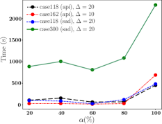
Figure 5: $\alpha$ sensitivity analysis for run times.

Improved QC relaxation gaps

TABLE I: QC relaxation gaps with trilinear functions relaxed using recursive McCormick (QC^rmc) vs. convex-hull representation (QC^conv).

Instances	QCrmc (%)	QCconv (%)
case3_lmbd	1.21	0.96
case30_ieee	15.64	15.20
case3_lmbd_api	1.79	1.59
case24_ieee_rts_api	11.88	8.78
case73_ieee_rts_api	10.97	9.64
case3_lmbd_sad	1.42	1.37
case4_gs_sad	1.53	0.96
case5_pjm_sad	0.99	0.77
case24_ieee_rts_sad	2.93	2.77
case73_ieee_rts_sad	2.53	2.38
case118_ieee_sad	4.61	4.14

Due to convex-hull relaxation of trilinear functions, the QC^conv gaps (highlighted in bold font in Table IV) outperformed the recursive McCormick approach used in [15]. Table I tabulates a few instances in which the improvements in QC gaps were significant based on the proposed approach. Even during bound-tightening, the best QC gaps using recursive McCormick (BT-QC^rmc) for trilinear functions were 2.7% and 11.8% for case30_fsr_api and case118_ieee_api, respectively. However, applying the convex-hull representation (BT-QC^conv) for the same instances significantly reduced the gaps to 0.35% and 8.54%, respectively.

VI-B Analyses of “Hard” Instances

In Table IV, there are 7 instances where the optimality gaps of BT-Lambda and BT-Lambda-$\alpha(60\%)$ are larger than 1%. These problems are hard because the tightened bounds remain weak. Table II shows that there are a large number of ${\theta}_{ij}$ variables whose bounds allow positive and negative values (flow could be in ether direction). This is generally not the case for the other instances. We also noticed that BT-Lambda has better gaps than BT-Lambda-$\alpha(60\%)$ in 5/35 instances. In this case, the heuristic incorrectly identifies variables whose partitioning is required to prove global optimality. To illustrate this, Table III counts the number of times a relaxed term does not have a variable that is partitioned (here, we use the lifted variable to refer to the term that is relaxed).

NCO instances AMP algorithm performed very well on 3/6 “nco” instances, hard for nonconvex optimization, where AMP finds near global optimum solutions within the time limits.

TABLE II: % of edges whose bounds are $(\boldsymbol{\underline{\theta}}<0)\wedge(\boldsymbol{\overline{\theta}}>0)$ after BT.

Instances	%
case240_wecc	77.6
case89_pegase_api	51.5
case118_ieee_api	32.4
case189_edin_api	33.0
case240_wecc_sad	68.1
case9_bgm_nco	44.4
case39_1_bgm_nco	45.7

TABLE III: Relaxed terms without partitions

Instances	$\widehat{w}$	$\widehat{cs}$	$\widehat{sn}$	$\widehat{wcs}$	$\widehat{wsn}$
case5_pjm	0	6	1	6	1
case240_wecc_sad	22	258	94	264	124
case9_na_cao_nco	1	9	1	9	4
case9_nb_cao_nco	1	9	1	9	3
case14_s_cao_nco	0	19	3	19	3

TABLE IV: The summary of performance NESTA 0.7.0 ACOPF instances. Values under “Gap” and “T,$T^{\alpha}$” are in % and seconds, respectively. “GOpt” refers to the global optimum when Gap $<0.01\%$. “TO” indicates time-out. “–” indicates no solution is provided under “SDP” and “Best of [6]” columns. “–” under “BT-Lambda” and “BT-Lambda-$\alpha$” columns indicates that the BT-QC^conv already converged to global optimum. Here, $\Delta^{*}$ represents the best one from {4, 6, 8, 10, 16} and $\alpha=60\%$.

							BT-Lambda		BT-Lambda–$\alpha(60\%)$
Instances	AC $(\$)$	QCconv (%)	SDP (%)	Best of [6] (%)	BTconv (s)	BT-QCconv (%)	($\Delta^{*}$) Gap	$T$	($\Delta^{*}$) Gap	$T^{\alpha}$
case3_lmbd	5812.64	0.97	0.39	0.09	2.1	GOpt	(16) GOpt	–	(16) GOpt	–
case5_pjm	17551.90	14.54	5.22	0.10	0.9	6.73	(6) GOpt	303.7	(6)  0.02	2023.6
case30_ieee	204.97	15.20	GOpt	–	48.1	GOpt	(16) GOpt	–	(16) GOpt	–
case118_ieee	3718.64	1.53	0.06	0.09	2235.0	GOpt	(10) GOpt	–	(20) GOpt	–
case162_ieee_dtc	4230.23	3.95	1.33	1.08	6292.3	GOpt	(10) GOpt	–	(10) GOpt	–
case240_wecc	75136.10	5.23	–	–	10800.0	2.90	(6)  2.64	TO	(16)  2.56	TO
case300_ieee	16891.28	1.17	0.08	0.19	10800.0	0.01	(20) GOpt	2164.2	(20) GOpt	1091.8
case3_lmbd_api	367.44	1.59	1.26	0.02	0.3	GOpt	(16) GOpt	–	(16) GOpt	–
case14_ieee_api	325.13	1.26	GOpt	0.09	11.7	0.06	(8) GOpt	0.4	(16) GOpt	0.04
case24_ieee_rts_api	6426.65	8.79	1.45	–	72.8	GOpt	(8) GOpt	–	(20) GOpt	–
case30_as_api	570.08	4.63	0.00	0.06	47.1	GOpt	(16) GOpt	–	(16) GOpt	–
case30_fsr_api	366.57	45.20	11.06	0.35	101.8	0.35	(6)  0.12	75.5	(8)  0.12	241.0
case39_epri_api	7460.37	2.97	GOpt	–	96.7	GOpt	(16) GOpt	–	(16) GOpt	–
case73_ieee_rts_api	19995.00	9.64	4.29	–	1528.2	0.01	(10) GOpt	61.2	(10) GOpt	27.8
case89_pegase_api	4255.44	19.83	18.11	–	3997.3	16.21	(6) 13.46	TO	(6) 13.08	TO
case118_ieee_api	10269.82	43.45	31.50	6.17	1515.6	8.54	(6)  4.19	TO	(6)  4.05	TO
case162_ieee_dtc_api	6106.86	1.25	0.85	1.03	6392.6	GOpt	(6) GOpt	–	(10) GOpt	–
case189_edin_api	1914.15	1.69	0.05	0.12	5110.9	0.04	(8)  0.03	2351.2	(8)  0.03	883.2
case3_lmbd_sad	5959.33	1.38	2.06	0.03	0.2	GOpt	(16) GOpt	–	(20) GOpt	–
case4_gs_sad	315.84	0.96	0.05	–	0.3	GOpt	(10) GOpt	–	(10) GOpt	–
case24_ieee_rts_sad	76943.24	2.77	6.05	–	44.7	GOpt	(6) GOpt	–	(16) GOpt	–
case29_edin_sad	41258.45	16.38	28.44	0.67	222.4	GOpt	(16) GOpt	–	(16) GOpt	–
case30_as_sad	897.49	2.32	0.47	0.08	53.8	GOpt	(16) GOpt	–	(16) GOpt	–
case30_ieee_sad	204.97	4.01	GOpt	0.08	50.4	GOpt	(16) GOpt	–	(16) GOpt	–
case73_ieee_rts_sad	227745.73	2.38	4.10	–	1655.8	GOpt	(6) GOpt	–	(20) GOpt	–
case118_ieee_sad	4106.72	4.15	7.57	2.43	2211.4	GOpt	(8) GOpt	–	(20) GOpt	–
case162_ieee_dtc_sad	4253.51	4.27	3.65	3.76	6337.2	0.01	(10) GOpt	88.5	(20) GOpt	41.7
case240_wecc_sad	76494.70	5.27	–	–	10800.0	2.61	(8)  2.41	TO	(16)  2.45	TO
case300_ieee_sad	16893.92	1.09	0.13	0.10	10800.0	GOpt	(10) GOpt	–	(20) GOpt	–
case5_bgm_nco	1082.33	10.17	–	–	6.93	GOpt	(6) GOpt	–	(8) GOpt	–
case9_bgm_nco	3087.84	10.84	–	–	2.72	10.80	(16) 10.12	7226.6	(20) 10.12	3017.1
case9_na_cao_nco	-212.43	-14.97	–	–	2.14	-6.90	(6) -0.04	58.6	(16) -0.73	31.4
case9_nb_cao_nco	-247.42	-15.59	–	–	2.62	-6.93	(6) -0.09	31.7	(8) -0.95	133.6
case14_s_cao_nco	9670.44	3.83	–	–	16.22	2.34	(6) 0.04	9626.2	(10)  0.07	4092.5
case39_1_bgm_nco	11221.00	3.72	–	–	103.98	3.58	(8) 3.46	14191.8	(10)  3.37	17090.3

VII Conclusions

This paper considered the classic ACOPF problem in polar form and developed efficient formulations and algorithms to solve it to global optimality. The key developments in this paper were a) Using state-of-the-art QC relaxations in combination with improved relaxations for trilinear functions based on the convex-hull representation, b) Developing novel mathematical formulations for tight piecewise convex relaxations of trilinear and quadratic functions, and c) Leveraging these tight formulations for global optimization using an adaptive multivariate partitioning approach in combination with bound tightening and effective heuristic branching strategies. Except in a few challenging instances, these methodologies helped to close the optimality gaps of many hard instances. Future directions include testing with other equivalent ACOPF formulations, exploitation of graph sparsitity, and better branching and pruning strategies for piecewise formulations.

References

- [1] M. B. Cain, R. P. O’neill, and A. Castillo, “History of optimal power flow and formulations,” Federal Energy Regulatory Commission, pp. 1–36, 2012.
- [2] J. Carpentier, “Contribution to the economic dispatch problem,” Bulletin de la Societe Francoise des Electriciens, vol. 3, no. 8, pp. 431–447, 1962.
- [3] G. P. McCormick, “Computability of global solutions to factorable nonconvex programs: Part I– convex underestimating problems,” Mathematical programming, vol. 10, no. 1, pp. 147–175, 1976.
- [4] H. Hijazi, C. Coffrin, and P. Van Hentenryck, “Convex quadratic relaxations for mixed-integer nonlinear programs in power systems,” Mathematical Programming - C, vol. 9, no. 3, pp. 321–367, 2017.
- [5] J. Lavaei and S. H. Low, “Zero duality gap in optimal power flow problem,” IEEE Trans. on Power Systems, vol. 27, no. 1, pp. 92–107, 2012.
- [6] B. Kocuk, S. S. Dey, and X. A. Sun, “Matrix minor reformulation and SOCP-based spatial branch-and-cut method for the AC optimal power flow problem,” arXiv preprint arXiv:1703.03050, 2017.
- [7] C. Coffrin, D. Gordon, and P. Scott, “NESTA, the NICTA energy system test case archive,” arXiv preprint arXiv:1411.0359, 2014.
- [8] A. Gopalakrishnan, A. U. Raghunathan, D. Nikovski, and L. T. Biegler, “Global optimization of optimal power flow using a branch & bound algorithm,” in 50th Annual Allerton Conference on Communication, Control, and Computing. IEEE, 2012, pp. 609–616.
- [9] H. Nagarajan, M. Lu, E. Yamangil, and R. Bent, “Tightening McCormick relaxations for nonlinear programs via dynamic multivariate partitioning,” in International Conference on Principles and Practice of Constraint Programming. Springer, 2016, pp. 369–387.
- [10] H. Nagarajan, M. Lu, S. Wang, R. Bent, and K. Sundar, “An adaptive, multivariate partitioning algorithm for global optimization of nonconvex programs,” arXiv preprint arXiv:1707.02514, 2017.
- [11] C. Coffrin, H. L. Hijazi, and P. Van Hentenryck, “Strengthening convex relaxations with bound tightening for power network optimization,” in International Conference on Principles and Practice of Constraint Programming. Springer, 2015, pp. 39–57.
- [12] C. Chen, A. Atamtürk, and S. S. Oren, “Bound tightening for the alternating current optimal power flow problem,” IEEE Trans. on Power Systems, vol. 31, no. 5, pp. 3729–3736, 2016.
- [13] F. Wu, H. Nagarajan, A. Zlotnik, R. Sioshansi, and A. M. Rudkevich, “Adaptive convex relaxations for gas pipeline network optimization,” in American Control Conference, 2017. IEEE, 2017, pp. 4710–4716.
- [14] M. Hasan and I. Karimi, “Piecewise linear relaxation of bilinear programs using bivariate partitioning,” AIChE journal, vol. 56, no. 7, pp. 1880–1893, 2010.
- [15] C. Coffrin, H. L. Hijazi, and P. Van Hentenryck, “The qc relaxation: A theoretical and computational study on optimal power flow,” IEEE Trans. on Power Systems, vol. 31, no. 4, pp. 3008–3018, 2016.
- [16] C. A. Meyer and C. A. Floudas, “Trilinear monomials with mixed sign domains: Facets of the convex and concave envelopes,” Journal of Global Optimization, vol. 29, no. 2, pp. 125–155, 2004.
- [17] A. D. Rikun, “A Convex Envelope Formula for Multilinear Functions,” Journal of Global Optimization, vol. 10, pp. 425–437, 1997.
- [18] M. Padberg, “Approximating separable nonlinear functions via mixed zero-one programs,” Operations Research Letters, vol. 27, no. 1, pp. 1–5, 2000.
- [19] J. P. Vielma, “Mixed integer linear programming formulation techniques,” SIAM Review, vol. 57, no. 1, pp. 3–57, 2015.
- [20] Y. Puranik and N. V. Sahinidis, “Domain reduction techniques for global NLP and MINLP optimization,” Constraints, pp. 1–39, 2017.
- [21] D. Bienstock and A. Verma, “Strong NP-hardness of AC power flows feasibility,” arXiv preprint arXiv:1512.07315, 2015.
- [22] J. Lee and D. Wilson, “Polyhedral methods for piecewise-linear functions i: the lambda method,” Discrete applied mathematics, vol. 108, no. 3, pp. 269–285, 2001.
- [23] I. Dunning, J. Huchette, and M. Lubin, “JuMP: A modeling language for mathematical optimization,” SIAM Review, vol. 59, no. 2, pp. 295–320, 2017.