Rational Approximation in the Bergman Spaces

Wei QU , Pei DANG Department of Information Technology, Macau University of Science and Technology. Email: 376928001@qq.com.
Department of Information Technology, Macau University of Science and Technology. Email: pdang@must.edu.mo.
Abstract

It is known that adaptive Fourier decomposition (AFD) offers efficient rational approximations to functions in the classical Hardy H2superscript𝐻2H^{2} spaces with significant applications. This study aims at rational approximation in Bergman, and more widely, in weighted Bergman spaces, the functions of which have more singularity than those in the Hardy spaces. Due to lack of an effective inner function theory, direct adaptation of the Hardy-space AFD is not performable. We, however, show that a pre-orthogonal method, being equivalent to AFD in the classical cases, is available for all weighted Bergman spaces. The theory in the Bergman spaces has equal force as AFD in the Hardy spaces. The methodology of approximation is via constructing the rational orthogonal systems of the Bergman type spaces, called Bergman space rational orthogonal (BRO) system, that have the same role as the Takennaka-Malmquist (TM) system in the Hardy spaces. Subsequently, we prove a certain type direct sum decomposition of the Bergman spaces that reveals the orthogonal complement relation between the span of the BRO system and the zero-based invariant spaces. We provide a sequence of examples with different and explicit singularities at the boundary along with a study on the inclusion relations of the weighted Bergman spaces. We finally present illustrative examples for effectiveness of the approximation.

1 Introduction

The aim of this work is to propose an adaptive approximation method in the weighted Bergman 𝔸α2subscriptsuperscript𝔸2𝛼\mathbb{A}^{2}_{\alpha} spaces analogous with the one established in the Hardy H2superscript𝐻2H^{2} spaces of the unit disc and the upper-half complex plane (classical contexts) called adaptive Fourier decomposition (AFD) [17]. The theory established in the Hardy spaces has direct applications in system identification and in signal analysis [13, 14, 19]. It is well known that a function f∈L2​(βˆ‚πƒ)𝑓superscript𝐿2𝐃f\in L^{2}(\partial\bf D) with Fourier expansion f​(ei​t)=βˆ‘βˆ’βˆžβˆžcn​ei​n​t𝑓superscript𝑒𝑖𝑑superscriptsubscriptsubscript𝑐𝑛superscript𝑒𝑖𝑛𝑑f(e^{it})=\sum_{-\infty}^{\infty}c_{n}e^{int} has its Hardy space decomposition f=f++fβˆ’,𝑓superscript𝑓superscript𝑓f=f^{+}+f^{-}, where f+​(ei​t)=βˆ‘0∞cn​ei​n​t∈H+2​(βˆ‚πƒ),superscript𝑓superscript𝑒𝑖𝑑superscriptsubscript0subscript𝑐𝑛superscript𝑒𝑖𝑛𝑑subscriptsuperscript𝐻2𝐃f^{+}(e^{it})=\sum_{0}^{\infty}c_{n}e^{int}\in H^{2}_{+}(\partial\bf D), and fβˆ’β€‹(ei​t)=βˆ‘βˆ’βˆžβˆ’1cn​ei​n​t∈Hβˆ’2​(βˆ‚πƒ).superscript𝑓superscript𝑒𝑖𝑑superscriptsubscript1subscript𝑐𝑛superscript𝑒𝑖𝑛𝑑subscriptsuperscript𝐻2𝐃f^{-}(e^{it})=\sum_{-\infty}^{-1}c_{n}e^{int}\in H^{2}_{-}(\partial\bf D). This decomposition corresponds to the space direct sum decomposition

L2​(βˆ‚πƒ)=𝐇+πŸβ€‹(βˆ‚πƒ)βŠ•π‡βˆ’πŸβ€‹(βˆ‚πƒ),superscript𝐿2𝐃direct-sumsubscriptsuperscript𝐇2𝐃subscriptsuperscript𝐇2𝐃\displaystyle L^{2}(\partial\bf D)=H^{2}_{+}(\partial\bf D)\oplus H^{2}_{-}(\partial\bf D), (1.1)

where HΒ±2​(βˆ‚πƒ)subscriptsuperscript𝐻2plus-or-minus𝐃H^{2}_{\pm}(\partial\bf D) are, correspondingly, the non-tangential boundary limits of the functions in the respective Hardy spaces inside and outside the unit disc, namely, HΒ±2​(𝐃).subscriptsuperscript𝐻2plus-or-minus𝐃H^{2}_{\pm}(\bf D). The projection operators from f𝑓f to HΒ±2​(𝐃)subscriptsuperscript𝐻2plus-or-minus𝐃H^{2}_{\pm}(\bf D) are, respectively, denoted as P±​(f)=(1/2)​(fΒ±i​H​fΒ±c0).subscript𝑃plus-or-minus𝑓12plus-or-minus𝑓𝑖𝐻𝑓subscript𝑐0P_{\pm}(f)=(1/2)(f\pm iHf\pm c_{0}). If f𝑓f is real-valued, due to the property cβˆ’n=cΒ―n,subscript𝑐𝑛subscript¯𝑐𝑛c_{-n}=\overline{c}_{n}, one has f=2​R​e​f+βˆ’c0.𝑓2Resuperscript𝑓subscript𝑐0f=2{\rm Re}f^{+}-c_{0}. The inverse operator of P+subscript𝑃P_{+} mapping f+superscript𝑓f^{+} to f𝑓f is invertible and bounded. Those suggest that analysis of the L2superscript𝐿2L^{2} functions may be reduced to analysis of the functions in the corresponding Hardy spaces [19]. Let {Bk}subscriptπ΅π‘˜\{B_{k}\} be the rational orthogonal system defined by a sequence of numbers 𝐚=(a1,β‹―,an,β‹―),𝐚subscriptπ‘Ž1β‹―subscriptπ‘Žπ‘›β‹―{\bf a}=(a_{1},\cdots,a_{n},\cdots), allowing repetition, in the unit disc of the form

Bk​(z)=1βˆ’|ak|21βˆ’aΒ―k​zβ€‹βˆl=1kβˆ’1zβˆ’al1βˆ’aΒ―l​z.subscriptπ΅π‘˜π‘§1superscriptsubscriptπ‘Žπ‘˜21subscriptΒ―π‘Žπ‘˜π‘§superscriptsubscriptproduct𝑙1π‘˜1𝑧subscriptπ‘Žπ‘™1subscriptΒ―π‘Žπ‘™π‘§B_{k}(z)=\frac{\sqrt{1-|a_{k}|^{2}}}{1-\overline{a}_{k}z}\prod_{l=1}^{k-1}\frac{z-a_{l}}{1-\overline{a}_{l}z}.

{Bk}k=1∞superscriptsubscriptsubscriptπ΅π‘˜π‘˜1\{B_{k}\}_{k=1}^{\infty} is an orthonormal system, also called Takenaka-Mulmquist or TM system, in H+2​(𝐃).subscriptsuperscript𝐻2𝐃H^{2}_{+}(\bf D). The system may or may not be a basis of H+2​(𝐃)subscriptsuperscript𝐻2𝐃H^{2}_{+}(\bf D) depending whether βˆ‘k=1∞(1βˆ’|ak|)=∞superscriptsubscriptπ‘˜11subscriptπ‘Žπ‘˜\sum_{k=1}^{\infty}(1-|a_{k}|)=\infty or not. In rational approximation in Hardy spaces one cannot avoid the above defined rational orthonormal systems for they are results of the Gram-Schmidt orthogonalization applied to partial fractions with different poles. Related to TM systems is the Beurling-Lax type direct sum decomposition

H2​(𝐃)=span¯​{𝐁𝐀}𝐀=πŸβˆžβŠ•Ο•β€‹π‡πŸβ€‹(𝐃),superscript𝐻2𝐃direct-sumΒ―spansuperscriptsubscriptsubscript𝐁𝐀𝐀1italic-Ο•superscript𝐇2𝐃\displaystyle H^{2}(\bf D)=\overline{{\rm span}}\{B_{k}\}_{k=1}^{\infty}\oplus\phi H^{2}(\bf D), (1.2)

where Ο•italic-Ο•\phi is the Blaschke product defined by the parameters a1,β‹―,ak,β‹―subscriptπ‘Ž1β‹―subscriptπ‘Žπ‘˜β‹―a_{1},\cdots,a_{k},\cdots. The validity of the last relation rests on the condition βˆ‘k=1∞(1βˆ’|ak|)<∞superscriptsubscriptπ‘˜11subscriptπ‘Žπ‘˜\sum_{k=1}^{\infty}(1-|a_{k}|)<\infty under which Ο•italic-Ο•\phi is well defined and the TM system is not a basis. Selecting parameters aksubscriptπ‘Žπ‘˜a_{k}’s under the maximal selection principle, regardless whether the corresponding TM system is a basis or not, the resulted AFD expansion

f+​(z)=βˆ‘k=1∞⟨f,BkβŸ©β€‹Bk​(z)superscript𝑓𝑧superscriptsubscriptπ‘˜1𝑓subscriptπ΅π‘˜subscriptπ΅π‘˜π‘§f^{+}(z)=\sum_{k=1}^{\infty}\langle f,B_{k}\rangle B_{k}(z)

converges at fast pace [17, 18]. One extra property, but important in signal analysis, of the decomposition is that under the selection a1=0subscriptπ‘Ž10a_{1}=0 all Bksubscriptπ΅π‘˜B_{k}’s are of positive frequencies (boundary phase derivative). AFD thus gives rise to intrinsic positive frequency decomposition of f+superscript𝑓f^{+} and thus that of f𝑓f as well. Other related work can be seen in [1, 20, 11]. In the analytic adaptive and positive-frequency approximation aspects the studies of Coifman et al. and Qian et al. merged together [3, 4].

To extend the theory of the Hardy spaces to the Bergman spaces a decomposition of L2​(𝐃)superscript𝐿2𝐃L^{2}(\bf D) similar to (1.1) with bounded invertible projections does not seem to be possible. Simple computation shows that the projection from L2​(𝐃)superscript𝐿2𝐃L^{2}(\bf D) to 𝔸2​(𝐃)superscript𝔸2𝐃\mathbb{A}^{2}(\bf D) is not one to one. The main task of this work is to explore the availability of (1.2) in the Bergman spaces case. The remarkable difference between the Hardy space and, for instance, the standard Bergman space is that

𝔸2​(𝐃)β‰ span¯​{𝐁𝐀}𝐀=πŸβˆžβŠ•Hπšβ€‹π”ΈπŸβ€‹(𝐃),superscript𝔸2𝐃direct-sumΒ―spansuperscriptsubscriptsubscript𝐁𝐀𝐀1subscript𝐻𝐚superscript𝔸2𝐃\displaystyle\mathbb{A}^{2}(\bf D)\neq\overline{\rm span}\{B_{k}\}_{k=1}^{\infty}\oplus{\it H}_{\bf a}\mathbb{A}^{2}(\bf D),

where {Bk}k=1∞superscriptsubscriptsubscriptπ΅π‘˜π‘˜1\{B_{k}\}_{k=1}^{\infty} is the Gram-Schmidt orthonormalization of a sequence of generalized reproducing kernels (see Β§2) corresponding to 𝐚𝐚{\bf a} that defines a Horowitz product H𝐚subscript𝐻𝐚H_{\bf a} [6] (see Β§2 and Β§5). On the other hand, we show that the direct sum decomposition holds with the Beurling type shift invariant subspace being replaced by the zero-based invariant subspace, that is

𝔸2​(𝐃)=span¯​{𝐁𝐀}𝐀=πŸβˆžβŠ•πˆπš.superscript𝔸2𝐃direct-sumΒ―spansuperscriptsubscriptsubscript𝐁𝐀𝐀1subscript𝐈𝐚\displaystyle\mathbb{A}^{2}(\bf D)=\overline{\rm span}\{B_{k}\}_{k=1}^{\infty}\oplus I_{\bf a}.

2 Preliminaries

Denote by 𝐃𝐃{\bf D} the open unit disc in the complex plane 𝐂.𝐂{\bf C}. We will first deal with the square integrable Bergman space of the open unit disc, 𝔸2​(𝐃),superscript𝔸2𝐃\mathbb{A}^{2}({\bf D}), namely,

𝔸2​(𝐃)={f:𝐃→𝐂|f​is​holomorphic​in​𝐃,πšπ§πβ€–f‖𝔸2​(𝐃)2=βˆ«πƒ|f​(z)|2​𝑑A<∞},superscript𝔸2𝐃conditional-set𝑓formulae-sequence→𝐃conditional𝐂𝑓isholomorphicinπƒπšπ§πsuperscriptsubscriptnorm𝑓superscript𝔸2𝐃2subscript𝐃superscript𝑓𝑧2differential-d𝐴\mathbb{A}^{2}({\bf D})=\{f:{\bf D}\to{\bf C}\ |\ f\ {\rm is\ holomorphic\ in\ \bf D,\ and\ }\ \|f\|_{\mathbb{A}^{2}({\bf D})}^{2}=\int_{\bf D}|f(z)|^{2}dA<\infty\},

where d​A𝑑𝐴dA is the normalized area measure on the unit disc: d​A=d​x​d​yΟ€,z=x+i​y.formulae-sequence𝑑𝐴𝑑π‘₯π‘‘π‘¦πœ‹π‘§π‘₯𝑖𝑦dA=\frac{dxdy}{\pi},z=x+iy. The space 𝔸2​(𝐃)superscript𝔸2𝐃\mathbb{A}^{2}({\bf D}) under the norm βˆ₯β‹…βˆ₯𝔸2​(𝐃)\|\cdot\|_{{\mathbb{A}^{2}}({\bf D})} forms a Hilbert space with the inner product

⟨f,gβŸ©π”Έ2​(𝐃)=βˆ«πƒf​(z)​g​(z)¯​𝑑A.subscript𝑓𝑔superscript𝔸2𝐃subscript𝐃𝑓𝑧¯𝑔𝑧differential-d𝐴\langle f,g\rangle_{\mathbb{A}^{2}({\bf D})}=\int_{\bf D}f(z)\overline{g(z)}dA.

In the sequel we often suppress the subscripts 𝔸2​(𝐃)superscript𝔸2𝐃\mathbb{A}^{2}({\bf D}) in the notations βˆ₯β‹…βˆ₯𝔸2​(𝐃)\|\cdot\|_{\mathbb{A}^{2}({\bf D})} and βŸ¨β‹…,β‹…βŸ©π”Έ2​(𝐃)subscriptβ‹…β‹…superscript𝔸2𝐃\langle\cdot,\cdot\rangle_{\mathbb{A}^{2}({\bf D})}, and write them simply as βˆ₯β‹…βˆ₯\|\cdot\| and βŸ¨β‹…,β‹…βŸ©.β‹…β‹…\langle\cdot,\cdot\rangle. We also write 𝔸2​(𝐃)superscript𝔸2𝐃\mathbb{A}^{2}({\bf D}) as 𝔸2superscript𝔸2\mathbb{A}^{2} [8, 6].

It is known that 𝔸2superscript𝔸2\mathbb{A}^{2} is a reproducing kernel Hilbert space with the reproducing kernel

ka​(z)=1(1βˆ’a¯​z)2.subscriptπ‘˜π‘Žπ‘§1superscript1Β―π‘Žπ‘§2k_{a}(z)=\frac{1}{(1-\overline{a}z)^{2}}.

From the reproducing kernel property we have

β€–kaβ€–2=ka​(a)=1(1βˆ’|a|2)2.superscriptnormsubscriptπ‘˜π‘Ž2subscriptπ‘˜π‘Žπ‘Ž1superscript1superscriptπ‘Ž22\|k_{a}\|^{2}=k_{a}(a)=\frac{1}{(1-|a|^{2})^{2}}.

Thus, the normalized reproducing kernel, denoted as ea​(z)subscriptπ‘’π‘Žπ‘§e_{a}(z), is

ea​(z)=ka​(z)ka​(a)=1βˆ’|a|2(1βˆ’a¯​z)2.subscriptπ‘’π‘Žπ‘§subscriptπ‘˜π‘Žπ‘§subscriptπ‘˜π‘Žπ‘Ž1superscriptπ‘Ž2superscript1Β―π‘Žπ‘§2e_{a}(z)=\frac{k_{a}(z)}{\sqrt{k_{a}(a)}}=\frac{1-|a|^{2}}{(1-\overline{a}z)^{2}}.

We hence have, for any fβˆˆπ”Έ2,𝑓superscript𝔸2f\in\mathbb{A}^{2},

⟨f,ea⟩=(1βˆ’|a|2)​f​(a).𝑓subscriptπ‘’π‘Ž1superscriptπ‘Ž2π‘“π‘Ž\langle f,e_{a}\rangle=(1-|a|^{2})f(a).

Let 𝐚𝐚{\bf a} be an infinite sequence with its elements in 𝐃,𝐃\bf D, that is 𝐚=(a1,β‹―,an,β‹―),anβˆˆπƒ,n=1,2,β‹―.formulae-sequence𝐚subscriptπ‘Ž1β‹―subscriptπ‘Žπ‘›β‹―formulae-sequencesubscriptπ‘Žπ‘›πƒπ‘›12β‹―{\bf a}=(a_{1},\cdots,a_{n},\cdots),a_{n}\in{\bf D},n=1,2,\cdots. Here, and in the sequel, ansubscriptπ‘Žπ‘›a_{n}’s are allowed to repeat. Denote by l​(an)𝑙subscriptπ‘Žπ‘›l(a_{n}) as the number of repeating time of the n𝑛n-th element ansubscriptπ‘Žπ‘›a_{n} of 𝐚nsubscriptπšπ‘›{\bf a}_{n} in the n𝑛n-tuple 𝐚n=(a1,β‹―,an).subscriptπšπ‘›subscriptπ‘Ž1β‹―subscriptπ‘Žπ‘›{\bf a}_{n}=(a_{1},\cdots,a_{n}). Denote by

k~an​(z)=(dd​wΒ―)(l​(an)βˆ’1)​(kw​(z))|w=an,subscript~π‘˜subscriptπ‘Žπ‘›π‘§evaluated-atsuperscript𝑑𝑑¯𝑀𝑙subscriptπ‘Žπ‘›1subscriptπ‘˜π‘€π‘§π‘€subscriptπ‘Žπ‘›\displaystyle\tilde{k}_{a_{n}}(z)=\left(\frac{d}{d\overline{w}}\right)^{(l(a_{n})-1)}\left(k_{w}(z)\right)|_{w=a_{n}}, (2.3)

that is, the (l​(an)βˆ’1)𝑙subscriptπ‘Žπ‘›1(l(a_{n})-1)-th derivative of kwsubscriptπ‘˜π‘€k_{w} with respect to the variable wΒ―,¯𝑀\overline{w}, then replace w𝑀w by an.subscriptπ‘Žπ‘›a_{n}. We will call the sequence {k~an}subscript~π‘˜subscriptπ‘Žπ‘›\{\tilde{k}_{a_{n}}\} the generalized reproducing kernels corresponding to (a1,β‹―,an)subscriptπ‘Ž1β‹―subscriptπ‘Žπ‘›(a_{1},\cdots,a_{n}).

We will be using the relation, for fβˆˆπ”Έ2,𝑓superscript𝔸2f\in\mathbb{A}^{2},

⟨f,k~an⟩=fl​(an)βˆ’1​(an).𝑓subscript~π‘˜subscriptπ‘Žπ‘›superscript𝑓𝑙subscriptπ‘Žπ‘›1subscriptπ‘Žπ‘›\displaystyle\langle f,\tilde{k}_{a_{n}}\rangle=f^{l(a_{n})-1}(a_{n}). (2.4)

To show (2.4), taking the (lβˆ’1)𝑙1(l-1) differentiation to the both sides of the identity

f​(w)=βˆ«πƒf​(z)(1βˆ’w​zΒ―)2​𝑑A,𝑓𝑀subscript𝐃𝑓𝑧superscript1𝑀¯𝑧2differential-d𝐴f(w)=\int_{\bf D}\frac{f(z)}{(1-w\overline{z})^{2}}dA,

we have

f(lβˆ’1)​(w)=l!β€‹βˆ«πƒzΒ―lβˆ’1​f​(z)(1βˆ’w​zΒ―)l+1​𝑑A.superscript𝑓𝑙1𝑀𝑙subscript𝐃superscript¯𝑧𝑙1𝑓𝑧superscript1𝑀¯𝑧𝑙1differential-d𝐴f^{(l-1)}(w)=l!\int_{\bf D}\frac{\overline{z}^{l-1}f(z)}{(1-w\overline{z})^{l+1}}dA.

The exchange of the order of differentiation and integration is justified by the Lebesgue Dominated Convergence Theorem based on the fact that the integrand does not have singularity. Taking into account

(dd​wΒ―)lβˆ’1¯​kw​(z)=(dd​w)lβˆ’1​kΒ―w​(z),Β―superscript𝑑𝑑¯𝑀𝑙1subscriptπ‘˜π‘€π‘§superscript𝑑𝑑𝑀𝑙1subscriptΒ―π‘˜π‘€π‘§\overline{\left(\frac{d}{d\overline{w}}\right)^{l-1}}k_{w}(z)=\left(\frac{d}{dw}\right)^{l-1}\overline{k}_{w}(z),

we obtain (2.4).

In various contexts, as well as in general reproducing kernel Hilbert spaces, including the Bergman spaces, this relation was noted by a number of authors [18, 16]. As revealed in the following sections, various degrees of differentiations of the kernel function correspond to times of repetitions of the parameters a1,…,an,…subscriptπ‘Ž1…subscriptπ‘Žπ‘›β€¦a_{1},...,a_{n},... Some literature for the clarity purpose deliberately avoid the repetition cases. To get the best approximations, repetition, however, is unavoidable and should be carefully treated.

We will be using the following functions, called Horowitz products, for aβˆˆπƒπ‘Žπƒa\in\bf D and 𝐚n=(a1,β‹―,an)βˆˆπƒπ§,subscriptπšπ‘›subscriptπ‘Ž1β‹―subscriptπ‘Žπ‘›superscript𝐃𝐧{\bf a}_{n}=(a_{1},\cdots,a_{n})\in\bf D^{n},

H{a}​(z)=|a|a​aβˆ’z1βˆ’a¯​z​(2βˆ’|a|a​aβˆ’z1βˆ’a¯​z)subscriptπ»π‘Žπ‘§π‘Žπ‘Žπ‘Žπ‘§1Β―π‘Žπ‘§2π‘Žπ‘Žπ‘Žπ‘§1Β―π‘Žπ‘§H_{\{a\}}(z)=\frac{|a|}{a}\frac{a-z}{1-\overline{a}z}\left(2-\frac{|a|}{a}\frac{a-z}{1-\overline{a}z}\right)

and

H𝐚n=H{a1}​⋯​H{an}.subscript𝐻subscriptπšπ‘›subscript𝐻subscriptπ‘Ž1β‹―subscript𝐻subscriptπ‘Žπ‘›H_{{\bf a}_{n}}=H_{\{a_{1}\}}\cdots H_{\{a_{n}\}}.

For 𝐚=(a1,β‹―,an,β‹―),𝐚subscriptπ‘Ž1β‹―subscriptπ‘Žπ‘›β‹―{\bf a}=(a_{1},\cdots,a_{n},\cdots), the condition

βˆ‘k=1∞(1βˆ’|ak|)2<∞superscriptsubscriptπ‘˜1superscript1subscriptπ‘Žπ‘˜2\displaystyle\sum_{k=1}^{\infty}(1-|a_{k}|)^{2}<\infty (2.5)

is necessary and sufficient for convergence of the corresponding infinite Horowitz product

Hπšβ€‹(z)=∏k=1∞H{ak}​(z),|z|<1.formulae-sequencesubscriptπ»πšπ‘§superscriptsubscriptproductπ‘˜1subscript𝐻subscriptπ‘Žπ‘˜π‘§π‘§1H_{\bf a}(z)=\prod_{k=1}^{\infty}H_{\{a_{k}\}}(z),\qquad|z|<1.

Under the condition the convergence is uniform for |z|≀rπ‘§π‘Ÿ|z|\leq r for any fixed 0<r<10π‘Ÿ10<r<1. It is noted that when the infinite product converges it does not have to converge to a function in the Bergman space [6].

We will study zero-based invariant subspaces. Let I𝐼I be a closed subspace of 𝔸2.superscript𝔸2\mathbb{A}^{2}. If further z​IβŠ‚I,𝑧𝐼𝐼zI\subset I, then we say that I𝐼I is an invariant subspace.

In the following we will concern the cases where I𝐼I corresponds to the set of functions that all vanish on an ordered set of points A,𝐴A, where the points of A𝐴A can repeat. Obviously such set I𝐼I is an invariant subspace, denoted as I=IA,𝐼subscript𝐼𝐴I=I_{A}, and is called the A𝐴A-zero based invariant subspace of 𝔸2::superscript𝔸2absent\mathbb{A}^{2}:

IA={fβˆˆπ”Έ2:f​has​all​points​in​A​as​its​zeros}.subscript𝐼𝐴conditional-set𝑓superscript𝔸2𝑓hasallpointsin𝐴asitszerosI_{A}=\{f\in\mathbb{A}^{2}\ :\ f\ {\rm has\ all\ points\ in\ }A\ {\rm as\ its\ zeros}\}.

In the above definition when a∈Aπ‘Žπ΄a\in A repeats l𝑙l times, by saying that f𝑓f takes value zero at all a∈Aπ‘Žπ΄a\in A we mean that f​(a)=f′​(a)=β‹―=f(lβˆ’1)​(a)=0.π‘“π‘Žsuperscriptπ‘“β€²π‘Žβ‹―superscript𝑓𝑙1π‘Ž0f(a)=f^{\prime}(a)=\cdots=f^{(l-1)}(a)=0. The fact f∈IA𝑓subscript𝐼𝐴f\in I_{A} is also denoted f​(A)=0.𝑓𝐴0f(A)=0. We will be interested in the case A=An=𝐚n=(a1,β‹―,an)𝐴subscript𝐴𝑛subscriptπšπ‘›subscriptπ‘Ž1β‹―subscriptπ‘Žπ‘›A=A_{n}={\bf a}_{n}=(a_{1},\cdots,a_{n}) and A=𝐚=(a1,β‹―,an,β‹―).𝐴𝐚subscriptπ‘Ž1β‹―subscriptπ‘Žπ‘›β‹―A={\bf a}=(a_{1},\cdots,a_{n},\cdots). Below we will denote Ο•a​(z)=zβˆ’a.subscriptitalic-Ο•π‘Žπ‘§π‘§π‘Ž\phi_{a}(z)=z-a. In the case I=I𝐚1=I{a1},𝐼subscript𝐼subscript𝐚1subscript𝐼subscriptπ‘Ž1I=I_{{\bf a}_{1}}=I_{\{a_{1}\}}, we can show that I{a1}=Ο•a1​𝔸2.subscript𝐼subscriptπ‘Ž1subscriptitalic-Ο•subscriptπ‘Ž1superscript𝔸2I_{\{a_{1}\}}=\phi_{a_{1}}\mathbb{A}^{2}. First, it is easy to see Ο•a1​𝔸2βŠ‚I{a1}.subscriptitalic-Ο•subscriptπ‘Ž1superscript𝔸2subscript𝐼subscriptπ‘Ž1\phi_{a_{1}}\mathbb{A}^{2}\subset I_{\{a_{1}\}}. On the other hand, if fβˆˆπ”Έ2𝑓superscript𝔸2f\in\mathbb{A}^{2} and f​(a1)=0,𝑓subscriptπ‘Ž10f(a_{1})=0, then f​(z)=Ο•a1​(z)​g​(z).𝑓𝑧subscriptitalic-Ο•subscriptπ‘Ž1𝑧𝑔𝑧f(z)=\phi_{a_{1}}(z)g(z). It is easy to show gβˆˆπ”Έ2.𝑔superscript𝔸2g\in\mathbb{A}^{2}. In fact, g𝑔g is analytic inside the disc 𝐃𝐃\bf D, and hence bounded in |z|≀|a1|+Ο΅<1.𝑧subscriptπ‘Ž1italic-Ο΅1|z|\leq|a_{1}|+\epsilon<1. Then

∫|z|≀|a1|+Ο΅|g​(z)|2​𝑑A​(z)<∞.subscript𝑧subscriptπ‘Ž1italic-Ο΅superscript𝑔𝑧2differential-d𝐴𝑧\int_{|z|\leq|a_{1}|+\epsilon}|g(z)|^{2}dA(z)<\infty.

On the other hand,

∫|a1|+Ο΅<|z|<1|g​(z)|2​𝑑A​(z)subscriptsubscriptπ‘Ž1italic-ϡ𝑧1superscript𝑔𝑧2differential-d𝐴𝑧\displaystyle\int_{|a_{1}|+\epsilon<|z|<1}|g(z)|^{2}dA(z) =\displaystyle= ∫|a1|+Ο΅<|z|<1|f​(z)|2|zβˆ’a1|2​𝑑A​(z)subscriptsubscriptπ‘Ž1italic-ϡ𝑧1superscript𝑓𝑧2superscript𝑧subscriptπ‘Ž12differential-d𝐴𝑧\displaystyle\int_{|a_{1}|+\epsilon<|z|<1}\frac{|f(z)|^{2}}{|z-a_{1}|^{2}}dA(z)
≀\displaystyle\leq 1Ο΅2β€‹βˆ«πƒ|f​(z)|2​𝑑A​(z)1superscriptitalic-Ο΅2subscript𝐃superscript𝑓𝑧2differential-d𝐴𝑧\displaystyle\frac{1}{\epsilon^{2}}\int_{\bf D}|{f(z)}|^{2}dA(z)
<\displaystyle< ∞.\displaystyle\infty.

Therefore, gβˆˆπ”Έ2,𝑔superscript𝔸2g\in\mathbb{A}^{2}, and I𝐚1βŠ‚Ο•a1​𝔸2.subscript𝐼subscript𝐚1subscriptitalic-Ο•subscriptπ‘Ž1superscript𝔸2I_{{\bf a}_{1}}\subset\phi_{a_{1}}\mathbb{A}^{2}. Inductively, we can show I𝐚n=Ο•a1​⋯​ϕan​𝔸2.subscript𝐼subscriptπšπ‘›subscriptitalic-Ο•subscriptπ‘Ž1β‹―subscriptitalic-Ο•subscriptπ‘Žπ‘›superscript𝔸2I_{{\bf a}_{n}}=\phi_{a_{1}}\cdots\phi_{a_{n}}\mathbb{A}^{2}. It is easy to see that H𝐚n​𝔸2subscript𝐻subscriptπšπ‘›superscript𝔸2H_{{\bf a}_{n}}\mathbb{A}^{2} is identical with Ο•a1​⋯​ϕan​𝔸2.subscriptitalic-Ο•subscriptπ‘Ž1β‹―subscriptitalic-Ο•subscriptπ‘Žπ‘›superscript𝔸2\phi_{a_{1}}\cdots\phi_{a_{n}}\mathbb{A}^{2}. Since the zero-based invariant spaces are closed subspaces, they themselves are reproducing kernel Hilbert spaces. When 𝐚𝐚{\bf a} is the zero set of some function fβˆˆπ”Έ2,𝑓superscript𝔸2f\in\mathbb{A}^{2}, then there holds the relation (2.5). An infinite sequence 𝐚𝐚{\bf a} satisfying condition (2.5), however, does not imply that it is the zero set of a function in the Bergman space. Necessary and sufficient conditions for 𝐚𝐚{\bf a} being the zero set of some Bergman space function is so far an open problem [9, 10, 15].

3 Rational Orthogonal System of 𝔸2superscript𝔸2\mathbb{A}^{2}

In this section we study rational orthogonal systems, or Takenaka-Malmquist systems as an alternative terminology, in the Bergman space. The following theorem is crucial. The scope of the following theorem is as the same as that in [21], except that multiples of the parameters are allowed. This generalization turns to be important for achieving the best approximation with the pre-orthogonal algorithm given in the next section (also see [16]).

Theorem 3.1

Let (a1,β‹―,an,β‹―)subscriptπ‘Ž1β‹―subscriptπ‘Žπ‘›β‹―(a_{1},\cdots,a_{n},\cdots) be an infinite sequence in 𝐃,𝐃\bf D, where each ansubscriptπ‘Žπ‘›a_{n} in the sequence is allowed to repeat. Let the orthonormalization of (k~a1,β‹―,k~an)subscript~π‘˜subscriptπ‘Ž1β‹―subscript~π‘˜subscriptπ‘Žπ‘›(\tilde{k}_{a_{1}},\cdots,\tilde{k}_{a_{n}}) be denoted (B1,…,Bn).subscript𝐡1…subscript𝐡𝑛(B_{1},...,B_{n}). Then for any n𝑛n, (i) the reproducing kernel of the zero-based invariant subspace IAnsubscript𝐼subscript𝐴𝑛I_{A_{n}} is

KAn​(z,w)=βˆ₯kwβˆ₯2βˆ’βˆ‘k=1n⟨kw,Bk⟩|2​Bn+1w,KA0​(z,w)=K​(z,w),K_{A_{n}}(z,w)=\sqrt{\|k_{w}\|^{2}-\sum_{k=1}^{n}\langle k_{w},B_{k}\rangle|^{2}}B_{n+1}^{w},\ K_{A_{0}}(z,w)=K(z,w),

where (B1,…,Bn,Bn+1w)subscript𝐡1…subscript𝐡𝑛superscriptsubscript𝐡𝑛1𝑀(B_{1},...,B_{n},B_{n+1}^{w}) is the orthonormalization of (k~a1,β‹―,k~an,kw),wsubscript~π‘˜subscriptπ‘Ž1β‹―subscript~π‘˜subscriptπ‘Žπ‘›subscriptπ‘˜π‘€π‘€(\tilde{k}_{a_{1}},\cdots,\tilde{k}_{a_{n}},k_{w}),w is none of a1,β‹―,an;subscriptπ‘Ž1β‹―subscriptπ‘Žπ‘›a_{1},\cdots,a_{n}; (ii) if an+1subscriptπ‘Žπ‘›1a_{n+1} coincides with some ak,k=1,β‹―,n,formulae-sequencesubscriptπ‘Žπ‘˜π‘˜1⋯𝑛a_{k},k=1,\cdots,n, that is, l​(an+1)>1,𝑙subscriptπ‘Žπ‘›11l(a_{n+1})>1, then Bn+1an+1superscriptsubscript𝐡𝑛1subscriptπ‘Žπ‘›1B_{n+1}^{a_{n+1}} is defined through

limwβ†’an+1Bn+1wsubscript→𝑀subscriptπ‘Žπ‘›1superscriptsubscript𝐡𝑛1𝑀\displaystyle\lim_{w\to a_{n+1}}B_{n+1}^{w} =\displaystyle= k~an+1​(z)βˆ’βˆ‘k=1n⟨k~an+1,BkβŸ©β€‹Bk​(z)β€–k~an+1βˆ’βˆ‘k=1n⟨k~an+1,BkβŸ©β€‹Bkβ€–subscript~π‘˜subscriptπ‘Žπ‘›1𝑧superscriptsubscriptπ‘˜1𝑛subscript~π‘˜subscriptπ‘Žπ‘›1subscriptπ΅π‘˜subscriptπ΅π‘˜π‘§normsubscript~π‘˜subscriptπ‘Žπ‘›1superscriptsubscriptπ‘˜1𝑛subscript~π‘˜subscriptπ‘Žπ‘›1subscriptπ΅π‘˜subscriptπ΅π‘˜\displaystyle\frac{\tilde{k}_{a_{n+1}}(z)-\sum_{k=1}^{n}\langle\tilde{k}_{a_{n+1}},B_{k}\rangle B_{k}(z)}{\|\tilde{k}_{a_{n+1}}-\sum_{k=1}^{n}\langle\tilde{k}_{a_{n+1}},B_{k}\rangle B_{k}\|}
=\displaystyle= k~an+1​(z)βˆ’βˆ‘k=1n⟨k~an+1,BkβŸ©β€‹Bk​(z)β€–kwβ€–2βˆ’βˆ‘k=1n|⟨k~an+1,Bk⟩|2,subscript~π‘˜subscriptπ‘Žπ‘›1𝑧superscriptsubscriptπ‘˜1𝑛subscript~π‘˜subscriptπ‘Žπ‘›1subscriptπ΅π‘˜subscriptπ΅π‘˜π‘§superscriptnormsubscriptπ‘˜π‘€2superscriptsubscriptπ‘˜1𝑛superscriptsubscript~π‘˜subscriptπ‘Žπ‘›1subscriptπ΅π‘˜2\displaystyle\frac{\tilde{k}_{a_{n+1}}(z)-\sum_{k=1}^{n}\langle\tilde{k}_{a_{n+1}},B_{k}\rangle B_{k}(z)}{\sqrt{\|k_{w}\|^{2}-\sum_{k=1}^{n}|\langle\tilde{k}_{a_{n+1}},B_{k}\rangle|^{2}}},

and thus Bn+1β‰œBn+1an+1.β‰œsubscript𝐡𝑛1superscriptsubscript𝐡𝑛1subscriptπ‘Žπ‘›1B_{n+1}\triangleq B_{n+1}^{a_{n+1}}.

Proof. (i) Let w𝑀w be none of a1,β‹―,an.subscriptπ‘Ž1β‹―subscriptπ‘Žπ‘›a_{1},\cdots,a_{n}. Under the Gram-Schmidt (G-S) orthonormalization process, Bn+1wsuperscriptsubscript𝐡𝑛1𝑀B_{n+1}^{w} is defined as

Bn+1w​(z)=kw​(z)βˆ’βˆ‘k=1n⟨kw,BkβŸ©β€‹Bk​(z)β€–kwβˆ’βˆ‘k=1n⟨kw,BkβŸ©β€‹Bkβ€–=kw​(z)βˆ’βˆ‘k=1n⟨kw,BkβŸ©β€‹Bk​(z)β€–kwβ€–2βˆ’βˆ‘k=1n|⟨kw,Bk⟩|2.superscriptsubscript𝐡𝑛1𝑀𝑧subscriptπ‘˜π‘€π‘§superscriptsubscriptπ‘˜1𝑛subscriptπ‘˜π‘€subscriptπ΅π‘˜subscriptπ΅π‘˜π‘§normsubscriptπ‘˜π‘€superscriptsubscriptπ‘˜1𝑛subscriptπ‘˜π‘€subscriptπ΅π‘˜subscriptπ΅π‘˜subscriptπ‘˜π‘€π‘§superscriptsubscriptπ‘˜1𝑛subscriptπ‘˜π‘€subscriptπ΅π‘˜subscriptπ΅π‘˜π‘§superscriptnormsubscriptπ‘˜π‘€2superscriptsubscriptπ‘˜1𝑛superscriptsubscriptπ‘˜π‘€subscriptπ΅π‘˜2\displaystyle B_{n+1}^{w}(z)=\frac{k_{w}(z)-\sum_{k=1}^{n}\langle k_{w},B_{k}\rangle B_{k}(z)}{\|k_{w}-\sum_{k=1}^{n}\langle k_{w},B_{k}\rangle B_{k}\|}=\frac{k_{w}(z)-\sum_{k=1}^{n}\langle k_{w},B_{k}\rangle B_{k}(z)}{\sqrt{\|k_{w}\|^{2}-\sum_{k=1}^{n}|\langle k_{w},B_{k}\rangle|^{2}}}. (3.6)

We are to show that

KAn​(β‹…,w)=β€–kwβ€–2βˆ’βˆ‘k=1n|⟨kw,Bk⟩|2​Bn+1w​(z)=kwβˆ’βˆ‘k=1n⟨kw,BkβŸ©β€‹Bk​(z)subscript𝐾subscript𝐴𝑛⋅𝑀superscriptnormsubscriptπ‘˜π‘€2superscriptsubscriptπ‘˜1𝑛superscriptsubscriptπ‘˜π‘€subscriptπ΅π‘˜2superscriptsubscript𝐡𝑛1𝑀𝑧subscriptπ‘˜π‘€superscriptsubscriptπ‘˜1𝑛subscriptπ‘˜π‘€subscriptπ΅π‘˜subscriptπ΅π‘˜π‘§K_{A_{n}}(\cdot,w)=\sqrt{\|k_{w}\|^{2}-\sum_{k=1}^{n}|\langle k_{w},B_{k}\rangle|^{2}}B_{n+1}^{w}(z)=k_{w}-\sum_{k=1}^{n}\langle k_{w},B_{k}\rangle B_{k}(z)

is the reproducing kernel of IAn.subscript𝐼subscript𝐴𝑛I_{A_{n}}. To this aim we first show (1) KAn​(β‹…,w)subscript𝐾subscript𝐴𝑛⋅𝑀K_{A_{n}}(\cdot,w) itself belongs to the space IAn;subscript𝐼subscript𝐴𝑛I_{A_{n}}; and then show (2) For f=Ο•a1​⋯​ϕan​g,gβˆˆπ”Έ2,formulae-sequence𝑓subscriptitalic-Ο•subscriptπ‘Ž1β‹―subscriptitalic-Ο•subscriptπ‘Žπ‘›π‘”π‘”superscript𝔸2f=\phi_{a_{1}}\cdots\phi_{a_{n}}g,g\in\mathbb{A}^{2}, there holds ⟨f,KAn​(β‹…,w)⟩=f​(w).𝑓subscript𝐾subscript𝐴𝑛⋅𝑀𝑓𝑀\langle f,K_{A_{n}}(\cdot,w)\rangle=f(w).

Now we show (1). From the construction of KAn​(β‹…,w)subscript𝐾subscript𝐴𝑛⋅𝑀K_{A_{n}}(\cdot,w) we know that it is orthogonal with all B1,⋯​Bn,subscript𝐡1β‹―subscript𝐡𝑛B_{1},\cdots B_{n}, and hence orthogonal with all k~a1,β‹―,k~an.subscript~π‘˜subscriptπ‘Ž1β‹―subscript~π‘˜subscriptπ‘Žπ‘›\tilde{k}_{a_{1}},\cdots,\tilde{k}_{a_{n}}. Let aπ‘Ža be a complex number appearing in the sequence (a1,β‹―,an)subscriptπ‘Ž1β‹―subscriptπ‘Žπ‘›(a_{1},\cdots,a_{n}) with the repetition number l.𝑙l. Then ka,βˆ‚βˆ‚w¯​ka,β‹―,(βˆ‚βˆ‚wΒ―)lβˆ’1​kasubscriptπ‘˜π‘ŽΒ―π‘€subscriptπ‘˜π‘Žβ‹―superscript¯𝑀𝑙1subscriptπ‘˜π‘Žk_{a},\frac{\partial}{\partial\overline{w}}k_{a},\cdots,\left(\frac{\partial}{\partial\overline{w}}\right)^{l-1}k_{a} will appear in k~a1,β‹―,k~an.subscript~π‘˜subscriptπ‘Ž1β‹―subscript~π‘˜subscriptπ‘Žπ‘›\tilde{k}_{a_{1}},\cdots,\tilde{k}_{a_{n}}. By invoking (2.4), the function KAn​(β‹…,w)subscript𝐾subscript𝐴𝑛⋅𝑀K_{A_{n}}(\cdot,w) being orthogonal with ka,βˆ‚βˆ‚w¯​ka,β‹―,(βˆ‚βˆ‚wΒ―)lβˆ’1​kasubscriptπ‘˜π‘ŽΒ―π‘€subscriptπ‘˜π‘Žβ‹―superscript¯𝑀𝑙1subscriptπ‘˜π‘Žk_{a},\frac{\partial}{\partial\overline{w}}k_{a},\cdots,\left(\frac{\partial}{\partial\overline{w}}\right)^{l-1}k_{a} means that KAn​(a,w)=βˆ‚βˆ‚z​KAn​(a,w)=β‹―=(βˆ‚βˆ‚z)lβˆ’1​KAn​(a,w)=0.subscript𝐾subscriptπ΄π‘›π‘Žπ‘€π‘§subscript𝐾subscriptπ΄π‘›π‘Žπ‘€β‹―superscript𝑧𝑙1subscript𝐾subscriptπ΄π‘›π‘Žπ‘€0K_{A_{n}}(a,w)=\frac{\partial}{\partial z}K_{A_{n}}(a,w)=\cdots=\left(\frac{\partial}{\partial z}\right)^{l-1}K_{A_{n}}(a,w)=0. The latter assertion further implies that KAn​(z,w)subscript𝐾subscript𝐴𝑛𝑧𝑀K_{A_{n}}(z,w) has the multiplicative factor (zβˆ’a)lsuperscriptπ‘§π‘Žπ‘™(z-a)^{l} and thus has the factor Ο•al.superscriptsubscriptitalic-Ο•π‘Žπ‘™\phi_{a}^{l}. By applying this argument for all aπ‘Ža appearing in the sequence (a1,β‹―,an)subscriptπ‘Ž1β‹―subscriptπ‘Žπ‘›(a_{1},\cdots,a_{n}) we obtain that for each w𝑀w, KAn​(β‹…,w)subscript𝐾subscript𝐴𝑛⋅𝑀K_{A_{n}}(\cdot,w) is in IAn.subscript𝐼subscript𝐴𝑛I_{A_{n}}.

Next we show (2), that is, for f=Ο•a1​⋯​ϕan​g,gβˆˆπ”Έ2,formulae-sequence𝑓subscriptitalic-Ο•subscriptπ‘Ž1β‹―subscriptitalic-Ο•subscriptπ‘Žπ‘›π‘”π‘”superscript𝔸2f=\phi_{a_{1}}\cdots\phi_{a_{n}}g,g\in\mathbb{A}^{2}, there holds ⟨f,KAn​(β‹…,w)⟩=f​(w).𝑓subscript𝐾subscript𝐴𝑛⋅𝑀𝑓𝑀\langle f,K_{A_{n}}(\cdot,w)\rangle=f(w). We first claim that

βŸ¨Ο•a1​⋯​ϕan​g,k~ak⟩=0,k=1,2,β‹―,n.formulae-sequencesubscriptitalic-Ο•subscriptπ‘Ž1β‹―subscriptitalic-Ο•subscriptπ‘Žπ‘›π‘”subscript~π‘˜subscriptπ‘Žπ‘˜0π‘˜12⋯𝑛\displaystyle\langle\phi_{a_{1}}\cdots\phi_{a_{n}}g,\tilde{k}_{a_{k}}\rangle=0,\ \ \ \ \ k=1,2,\cdots,n. (3.7)

Let aksubscriptπ‘Žπ‘˜a_{k} repeat l𝑙l times in (a1,β‹―,an)subscriptπ‘Ž1β‹―subscriptπ‘Žπ‘›(a_{1},\cdots,a_{n})\ and l​(ak)𝑙subscriptπ‘Žπ‘˜l(a_{k}) times in (a1,β‹―,ak).subscriptπ‘Ž1β‹―subscriptπ‘Žπ‘˜(a_{1},\cdots,a_{k}). We always have lβ‰₯l​(ak).𝑙𝑙subscriptπ‘Žπ‘˜l\geq l(a_{k}). In such notation the factor(Ο•ak)lsuperscriptsubscriptitalic-Ο•subscriptπ‘Žπ‘˜π‘™(\phi_{a_{k}})^{l} lies in Ο•a1​⋯​ϕansubscriptitalic-Ο•subscriptπ‘Ž1β‹―subscriptitalic-Ο•subscriptπ‘Žπ‘›\phi_{a_{1}}\cdots\phi_{a_{n}} and for some hβˆˆπ”Έ2,Ο•akl​h=Ο•a1​⋯​ϕan​g.formulae-sequenceβ„Žsuperscript𝔸2subscriptsuperscriptitalic-ϕ𝑙subscriptπ‘Žπ‘˜β„Žsubscriptitalic-Ο•subscriptπ‘Ž1β‹―subscriptitalic-Ο•subscriptπ‘Žπ‘›π‘”h\in\mathbb{A}^{2},\ \phi^{l}_{a_{k}}h=\phi_{a_{1}}\cdots\phi_{a_{n}}g. By (2.4), we have

βŸ¨Ο•a1​⋯​ϕan​g,k~ak⟩subscriptitalic-Ο•subscriptπ‘Ž1β‹―subscriptitalic-Ο•subscriptπ‘Žπ‘›π‘”subscript~π‘˜subscriptπ‘Žπ‘˜\displaystyle\langle\phi_{a_{1}}\cdots\phi_{a_{n}}g,\tilde{k}_{a_{k}}\rangle =\displaystyle= βŸ¨Ο•akl​h,(βˆ‚βˆ‚wΒ―)l​(ak)βˆ’1​kw⟩|w=akevaluated-atsubscriptsuperscriptitalic-ϕ𝑙subscriptπ‘Žπ‘˜β„Žsuperscript¯𝑀𝑙subscriptπ‘Žπ‘˜1subscriptπ‘˜π‘€π‘€subscriptπ‘Žπ‘˜\displaystyle\langle\phi^{l}_{a_{k}}h,\left(\frac{\partial}{\partial\overline{w}}\right)^{l(a_{k})-1}k_{w}\rangle|_{w=a_{k}}
=\displaystyle= (Ο•akl​h)(l​(ak)βˆ’1)​(ak)superscriptsubscriptsuperscriptitalic-ϕ𝑙subscriptπ‘Žπ‘˜β„Žπ‘™subscriptπ‘Žπ‘˜1subscriptπ‘Žπ‘˜\displaystyle(\phi^{l}_{a_{k}}h)^{(l(a_{k})-1)}(a_{k})
=\displaystyle= 0.0\displaystyle 0.

Since each Bksubscriptπ΅π‘˜B_{k} is a linear combination of (k~a1,β‹―,k~ak),subscript~π‘˜subscriptπ‘Ž1β‹―subscript~π‘˜subscriptπ‘Žπ‘˜(\tilde{k}_{a_{1}},\cdots,\tilde{k}_{a_{k}}), we have, owing to (3.7),

βŸ¨Ο•a1​⋯​ϕan​g,Kn​(β‹…,w)⟩subscriptitalic-Ο•subscriptπ‘Ž1β‹―subscriptitalic-Ο•subscriptπ‘Žπ‘›π‘”subscript𝐾𝑛⋅𝑀\displaystyle\langle\phi_{a_{1}}\cdots\phi_{a_{n}}g,K_{n}(\cdot,w)\rangle =\displaystyle= βŸ¨Ο•a1​⋯​ϕan​g,kwβˆ’βˆ‘k=1n⟨kw,BkβŸ©β€‹Bk​(z)⟩subscriptitalic-Ο•subscriptπ‘Ž1β‹―subscriptitalic-Ο•subscriptπ‘Žπ‘›π‘”subscriptπ‘˜π‘€superscriptsubscriptπ‘˜1𝑛subscriptπ‘˜π‘€subscriptπ΅π‘˜subscriptπ΅π‘˜π‘§\displaystyle\langle\phi_{a_{1}}\cdots\phi_{a_{n}}g,k_{w}-\sum_{k=1}^{n}\langle k_{w},B_{k}\rangle B_{k}(z)\rangle
=\displaystyle= βŸ¨Ο•a1​⋯​ϕan​g,kw⟩+βˆ‘k=1nckβ€‹βŸ¨Ο•a1​⋯​ϕan​g,k~ak⟩subscriptitalic-Ο•subscriptπ‘Ž1β‹―subscriptitalic-Ο•subscriptπ‘Žπ‘›π‘”subscriptπ‘˜π‘€superscriptsubscriptπ‘˜1𝑛subscriptπ‘π‘˜subscriptitalic-Ο•subscriptπ‘Ž1β‹―subscriptitalic-Ο•subscriptπ‘Žπ‘›π‘”subscript~π‘˜subscriptπ‘Žπ‘˜\displaystyle\langle\phi_{a_{1}}\cdots\phi_{a_{n}}g,k_{w}\rangle+\sum_{k=1}^{n}c_{k}\langle\phi_{a_{1}}\cdots\phi_{a_{n}}g,\tilde{k}_{a_{k}}\rangle
=\displaystyle= Ο•a1​(w)​⋯​ϕan​(w)​g​(w)subscriptitalic-Ο•subscriptπ‘Ž1𝑀⋯subscriptitalic-Ο•subscriptπ‘Žπ‘›π‘€π‘”π‘€\displaystyle\phi_{a_{1}}(w)\cdots\phi_{a_{n}}(w)g(w)
=\displaystyle= f​(w).𝑓𝑀\displaystyle f(w).

Therefore, Kn​(z,w)subscript𝐾𝑛𝑧𝑀K_{n}(z,w) is the reproducing kernel of IAn.subscript𝐼subscript𝐴𝑛I_{A_{n}}. The proof of (2) is complete.

Now we prove (ii) that treats l=l​(an+1)>1.𝑙𝑙subscriptπ‘Žπ‘›11l=l(a_{n+1})>1. This means that, with a little abuse of notation, the lβˆ’1𝑙1l-1 terms kan+1,βˆ‚βˆ‚w¯​kan+1,β‹―,subscriptπ‘˜subscriptπ‘Žπ‘›1¯𝑀subscriptπ‘˜subscriptπ‘Žπ‘›1β‹―k_{a_{n+1}},\frac{\partial}{\partial\overline{w}}k_{a_{n+1}},\cdots, (βˆ‚βˆ‚wΒ―)(lβˆ’2)​kan+1superscript¯𝑀𝑙2subscriptπ‘˜subscriptπ‘Žπ‘›1\left(\frac{\partial}{\partial\overline{w}}\right)^{(l-2)}k_{a_{n+1}} as functions of the z𝑧z variable have appeared in the sequence (k~a1,β‹―,k~an).subscript~π‘˜subscriptπ‘Ž1β‹―subscript~π‘˜subscriptπ‘Žπ‘›(\tilde{k}_{a_{1}},\cdots,\tilde{k}_{a_{n}}). Therefore, the function

kan+1+βˆ‚βˆ‚w¯​kan+11!​(wΒ―βˆ’aΒ―n+1)+β‹―+(βˆ‚βˆ‚wΒ―)(lβˆ’2)​kan+1(lβˆ’2)!​(wΒ―βˆ’aΒ―n+1)lβˆ’2,subscriptπ‘˜subscriptπ‘Žπ‘›1¯𝑀subscriptπ‘˜subscriptπ‘Žπ‘›11¯𝑀subscriptΒ―π‘Žπ‘›1β‹―superscript¯𝑀𝑙2subscriptπ‘˜subscriptπ‘Žπ‘›1𝑙2superscript¯𝑀subscriptΒ―π‘Žπ‘›1𝑙2k_{a_{n+1}}+\frac{\frac{\partial}{\partial\overline{w}}k_{a_{n+1}}}{1!}(\overline{w}-\overline{a}_{n+1})+\cdots+\frac{\left(\frac{\partial}{\partial\overline{w}}\right)^{(l-2)}k_{a_{n+1}}}{(l-2)!}(\overline{w}-\overline{a}_{n+1})^{l-2},

as the order-(lβˆ’2)𝑙2(l-2) Taylor expansion of the function kw​(z)subscriptπ‘˜π‘€π‘§k_{w}(z) with respect to the variable w¯¯𝑀\overline{w} at wΒ―=aΒ―n+1,¯𝑀subscriptΒ―π‘Žπ‘›1\overline{w}=\overline{a}_{n+1}, is already in the linear span of B1,β‹―,Bn.subscript𝐡1β‹―subscript𝐡𝑛B_{1},\cdots,B_{n}. Denoting the Taylor expansion by Tlβˆ’2​(kw,an+1),subscript𝑇𝑙2subscriptπ‘˜π‘€subscriptπ‘Žπ‘›1T_{l-2}(k_{w},a_{n+1}), the last mentioned assertion amounts to the relation

Tlβˆ’2​(kw,an+1)βˆ’βˆ‘k=1n⟨Tlβˆ’2​(kw,an+1),BkβŸ©β€‹Bk=0.subscript𝑇𝑙2subscriptπ‘˜π‘€subscriptπ‘Žπ‘›1superscriptsubscriptπ‘˜1𝑛subscript𝑇𝑙2subscriptπ‘˜π‘€subscriptπ‘Žπ‘›1subscriptπ΅π‘˜subscriptπ΅π‘˜0\displaystyle T_{l-2}(k_{w},a_{n+1})-\sum_{k=1}^{n}\langle T_{l-2}(k_{w},a_{n+1}),B_{k}\rangle B_{k}=0. (3.8)

For w𝑀w being different from all ak,k=1,β‹―,n,formulae-sequencesubscriptπ‘Žπ‘˜π‘˜1⋯𝑛a_{k},k=1,\cdots,n, we have, owing to (3.6),

kw​(z)βˆ’βˆ‘k=1n⟨kw,BkβŸ©β€‹Bk​(z)β€–kwβˆ’βˆ‘k=1n⟨kw,BkβŸ©β€‹Bkβ€–=Bn+1w​(z),subscriptπ‘˜π‘€π‘§superscriptsubscriptπ‘˜1𝑛subscriptπ‘˜π‘€subscriptπ΅π‘˜subscriptπ΅π‘˜π‘§normsubscriptπ‘˜π‘€superscriptsubscriptπ‘˜1𝑛subscriptπ‘˜π‘€subscriptπ΅π‘˜subscriptπ΅π‘˜superscriptsubscript𝐡𝑛1𝑀𝑧\displaystyle\frac{k_{w}(z)-\sum_{k=1}^{n}\langle k_{w},B_{k}\rangle B_{k}(z)}{\|k_{w}-\sum_{k=1}^{n}\langle k_{w},B_{k}\rangle B_{k}\|}=B_{n+1}^{w}(z), (3.9)

Inserting (3.8) into (3.9), and dividing by (wΒ―βˆ’aΒ―n+1)lβˆ’1superscript¯𝑀subscriptΒ―π‘Žπ‘›1𝑙1(\overline{w}-\overline{a}_{n+1})^{l-1} and |wΒ―βˆ’aΒ―n+1|lβˆ’1superscript¯𝑀subscriptΒ―π‘Žπ‘›1𝑙1|\overline{w}-\overline{a}_{n+1}|^{l-1} to the numerator and the denominator, respectively, we have

eβˆ’(lβˆ’1)​θ​kw​(z)βˆ’Tlβˆ’2​(kw,an+1)​(z)(wΒ―βˆ’aΒ―n+1)lβˆ’1βˆ’βˆ‘k=1n⟨kwβˆ’Tlβˆ’2​(kw,an+1)​(z)wΒ―βˆ’aΒ―n+1)lβˆ’1,BkβŸ©β€‹Bk​(z)β€–kw​(z)βˆ’Tlβˆ’2​(kw,an+1)​(z)(wΒ―βˆ’aΒ―n+1)lβˆ’1βˆ’βˆ‘k=1n⟨kw​(z)βˆ’Tlβˆ’2​(kw,an+1)​(z)(wΒ―βˆ’aΒ―n+1)lβˆ’1,BkβŸ©β€‹Bkβ€–=Bn+1w​(z),\displaystyle e^{-(l-1)\theta}\frac{\frac{k_{w}(z)-T_{l-2}(k_{w},a_{n+1})(z)}{(\overline{w}-\overline{a}_{n+1})^{l-1}}-\sum_{k=1}^{n}\langle\frac{k_{w}-T_{l-2}(k_{w},a_{n+1})(z)}{\overline{w}-\overline{a}_{n+1})^{l-1}},B_{k}\rangle B_{k}(z)}{\|\frac{k_{w}(z)-T_{l-2}(k_{w},a_{n+1})(z)}{(\overline{w}-\overline{a}_{n+1})^{l-1}}-\sum_{k=1}^{n}\langle\frac{k_{w}(z)-T_{l-2}(k_{w},a_{n+1})(z)}{(\overline{w}-\overline{a}_{n+1})^{l-1}},B_{k}\rangle B_{k}\|}=B_{n+1}^{w}(z), (3.10)

where wΒ―βˆ’aΒ―n+1=|wΒ―βˆ’aΒ―n+1|​ei​θ.¯𝑀subscriptΒ―π‘Žπ‘›1¯𝑀subscriptΒ―π‘Žπ‘›1superscriptπ‘’π‘–πœƒ\overline{w}-\overline{a}_{n+1}=|\overline{w}-\overline{a}_{n+1}|e^{i\theta}. Letting wβ†’an+1→𝑀subscriptπ‘Žπ‘›1w\to a_{n+1}, keeping the direction ei​θ,superscriptπ‘’π‘–πœƒe^{i\theta}, and using the Lagrange type remainder, we obtain

eβˆ’(lβˆ’1)​θ​k~an+1​(z)βˆ’βˆ‘k=1n⟨k~an+1,BkβŸ©β€‹Bk​(z)β€–k~an+1βˆ’βˆ‘k=1n⟨k~an+1,BkβŸ©β€‹Bkβ€–=Bn+1​(z).superscript𝑒𝑙1πœƒsubscript~π‘˜subscriptπ‘Žπ‘›1𝑧superscriptsubscriptπ‘˜1𝑛subscript~π‘˜subscriptπ‘Žπ‘›1subscriptπ΅π‘˜subscriptπ΅π‘˜π‘§normsubscript~π‘˜subscriptπ‘Žπ‘›1superscriptsubscriptπ‘˜1𝑛subscript~π‘˜subscriptπ‘Žπ‘›1subscriptπ΅π‘˜subscriptπ΅π‘˜subscript𝐡𝑛1𝑧e^{-(l-1)\theta}\frac{\tilde{k}_{a_{n+1}}(z)-\sum_{k=1}^{n}\langle\tilde{k}_{a_{n+1}},B_{k}\rangle B_{k}(z)}{\|\tilde{k}_{a_{n+1}}-\sum_{k=1}^{n}\langle\tilde{k}_{a_{n+1}},B_{k}\rangle B_{k}\|}=B_{n+1}(z).

This shows that the G-S orthonormalization of (k~a1,β‹―,k~an+1)subscript~π‘˜subscriptπ‘Ž1β‹―subscript~π‘˜subscriptπ‘Žπ‘›1(\tilde{k}_{a_{1}},\cdots,\tilde{k}_{a_{n+1}}) is (B1,β‹―,Bn+1).subscript𝐡1β‹―subscript𝐡𝑛1(B_{1},\cdots,B_{n+1}). The proof of (ii) is complete.


We call (B1,β‹―,Bn,β‹―)subscript𝐡1β‹―subscript𝐡𝑛⋯(B_{1},\cdots,B_{n},\cdots) the rational orthonormal system or the Takenaka-Malmquist system (TM system) of the Bergman space associated with the infinite sequence (a,​⋯,an,β‹―)subscriptπ‘Ž,β‹―subscriptπ‘Žπ‘›β‹―(a_{,}\cdots,a_{n},\cdots) or, equivalently, the generalized reproducing kernels sequence (k~a1,β‹―,k~an,β‹―),subscript~π‘˜subscriptπ‘Ž1β‹―subscript~π‘˜subscriptπ‘Žπ‘›β‹―(\tilde{k}_{a_{1}},\cdots,\tilde{k}_{a_{n}},\cdots), where for each n𝑛n, (B1,β‹―,Bn)subscript𝐡1β‹―subscript𝐡𝑛(B_{1},\cdots,B_{n}) is the Gram-Schmidt orthonormalization of (k~a1,β‹―,k~an).subscript~π‘˜subscriptπ‘Ž1β‹―subscript~π‘˜subscriptπ‘Žπ‘›(\tilde{k}_{a_{1}},\cdots,\tilde{k}_{a_{n}}). For fixed a1,β‹―,an,subscriptπ‘Ž1β‹―subscriptπ‘Žπ‘›a_{1},\cdots,a_{n}, the correspondence between an+1subscriptπ‘Žπ‘›1a_{n+1} and Bn+1subscript𝐡𝑛1B_{n+1} is unique up to a multiplicative constant of complex modular 1.11.

4 Pre-Orthogonal Adaptive Fourier Decomposition of the Bergman Space 𝔸2superscript𝔸2\mathbb{A}^{2}

The purpose of this section is to introduce a machinery that gives rise to fast rational approximation to functions in the Bergman space. The machinery is an adaptation of a general method called pre-orthogonal adaptive Fourier decomposition or POAFD for certain Hilbert spaces possessing the boundary vanish property [16]. The major work of this section is to verify the boundary vanishing condition of the Bergman space. It is the pre-orthogonal process that requires repeating selections of the parameter a,π‘Ža, when necessary, and therefore the necessity of the derivatives of the reproducing kernel.

Let fβˆˆπ”Έ2.𝑓superscript𝔸2f\in\mathbb{A}^{2}. Denoting f=f1.𝑓subscript𝑓1f=f_{1}. For the normalized reproducing kernel easubscriptπ‘’π‘Že_{a} for any aβˆˆπƒ,π‘Žπƒa\in\bf D, we have the identity

f​(z)=⟨f1,ea1βŸ©β€‹ea1​(z)+f2​(z),𝑓𝑧subscript𝑓1subscript𝑒subscriptπ‘Ž1subscript𝑒subscriptπ‘Ž1𝑧subscript𝑓2𝑧f(z)=\langle f_{1},e_{a_{1}}\rangle e_{a_{1}}(z)+f_{2}(z),

where f2=f1βˆ’βŸ¨f1,ea1βŸ©β€‹ea1subscript𝑓2subscript𝑓1subscript𝑓1subscript𝑒subscriptπ‘Ž1subscript𝑒subscriptπ‘Ž1f_{2}=f_{1}-\langle f_{1},e_{a_{1}}\rangle e_{a_{1}} is orthogonal with ea1.subscript𝑒subscriptπ‘Ž1e_{a_{1}}. The last assertion is proved through the Hilbert space projection property. We also have

β€–fβ€–2=|⟨f1,ea1⟩|2+β€–f2β€–2.superscriptnorm𝑓2superscriptsubscript𝑓1subscript𝑒subscriptπ‘Ž12superscriptnormsubscript𝑓22\|f\|^{2}=|\langle f_{1},e_{a_{1}}\rangle|^{2}+\|f_{2}\|^{2}.

The strategy is to maximize the value of |⟨f1,ea1⟩|2superscriptsubscript𝑓1subscript𝑒subscriptπ‘Ž12|\langle f_{1},e_{a_{1}}\rangle|^{2} through selections of a1,subscriptπ‘Ž1a_{1}, and thus to minimize the energy of f2.subscript𝑓2f_{2}. Despite of the fact that 𝐃𝐃{\bf D} is an open set, we have

Lemma 4.1

For any fβˆˆπ”Έ2𝑓superscript𝔸2f\in\mathbb{A}^{2} there exists aβˆˆπƒπ‘Žπƒa\in{\bf D} such that

|⟨f,ea⟩|2=max⁑{|⟨f,eb⟩|2:bβˆˆπƒ}.superscript𝑓subscriptπ‘’π‘Ž2:superscript𝑓subscript𝑒𝑏2𝑏𝐃|\langle f,e_{a}\rangle|^{2}=\max\{|\langle f,e_{b}\rangle|^{2}\ :\ b\in{\bf D}\}.

Proof The Cauchy-Schwarz inequality gives

|⟨f,eb⟩|≀‖fβ€–.𝑓subscript𝑒𝑏norm𝑓|\langle f,e_{b}\rangle|\leq\|f\|.

Therefore |⟨f,eb⟩|𝑓subscript𝑒𝑏|\langle f,e_{b}\rangle| has a finite upper bound.

For Ο΅>0,italic-Ο΅0\epsilon>0, since polynomials are dense in the Bergman space, there exists a polynomial g𝑔g such that

β€–fβˆ’g‖≀ϡ.norm𝑓𝑔italic-Ο΅\|f-g\|\leq\epsilon.

The Cauchy-Schwarz inequality gives

|⟨f,eb⟩|≀|⟨g,eb⟩|+Ο΅=(1βˆ’|b|2)​|g​(b)|+Ο΅.𝑓subscript𝑒𝑏𝑔subscript𝑒𝑏italic-Ο΅1superscript𝑏2𝑔𝑏italic-Ο΅|\langle f,e_{b}\rangle|\leq|\langle g,e_{b}\rangle|+\epsilon=(1-|b|^{2})|g(b)|+\epsilon.

The last quantity tends to zero as |b|β†’1.→𝑏1|b|\to 1. Therefore |⟨f,eb⟩|𝑓subscript𝑒𝑏|\langle f,e_{b}\rangle| attains the maximum value at an interior point.   

For f1βˆˆπ”Έ2subscript𝑓1superscript𝔸2f_{1}\in\mathbb{A}^{2} choose a1subscriptπ‘Ž1a_{1} such that

|⟨f1,ea1⟩|2=max⁑{|⟨f1,eb⟩|2:bβˆˆπƒ}.superscriptsubscript𝑓1subscript𝑒subscriptπ‘Ž12:superscriptsubscript𝑓1subscript𝑒𝑏2𝑏𝐃|\langle f_{1},e_{a_{1}}\rangle|^{2}=\max\{|\langle f_{1},e_{b}\rangle|^{2}\ :\ b\in{\bf D}\}.

Fixing such a1,subscriptπ‘Ž1a_{1}, we have, by denoting ea1=B1,subscript𝑒subscriptπ‘Ž1subscript𝐡1e_{a_{1}}=B_{1},

f​(z)=⟨f1,B1βŸ©β€‹B1​(z)+⟨f2,B2bβŸ©β€‹B2b​(z)+f3,𝑓𝑧subscript𝑓1subscript𝐡1subscript𝐡1𝑧subscript𝑓2superscriptsubscript𝐡2𝑏superscriptsubscript𝐡2𝑏𝑧subscript𝑓3\displaystyle f(z)=\langle f_{1},B_{1}\rangle B_{1}(z)+\langle f_{2},B_{2}^{b}\rangle B_{2}^{b}(z)+f_{3}, (4.11)

where (B1,B2b)subscript𝐡1superscriptsubscript𝐡2𝑏(B_{1},B_{2}^{b}) is the G-S orthonormalization of (B1,k~b).subscript𝐡1subscript~π‘˜π‘(B_{1},\tilde{k}_{b}). In the end of the argument we will not exclude the case b=a1,𝑏subscriptπ‘Ž1b=a_{1}, but for the time being we assume bβ‰ a1.𝑏subscriptπ‘Ž1b\neq a_{1}. By invoking the formula (3.6) and the orthogonality between f2subscript𝑓2f_{2} and B1,subscript𝐡1B_{1}, we have

⟨f2,B2b⟩=⟨f2,eb1βˆ’|⟨eb,B1⟩|2⟩subscript𝑓2superscriptsubscript𝐡2𝑏subscript𝑓2subscript𝑒𝑏1superscriptsubscript𝑒𝑏subscript𝐡12\displaystyle\langle f_{2},B_{2}^{b}\rangle=\langle f_{2},\frac{e_{b}}{\sqrt{1-|\langle e_{b},B_{1}\rangle|^{2}}}\rangle

The corresponding integral, first, has a finite upper bound independent of bβˆˆπƒ.𝑏𝐃b\in{\bf D}. We will show that the norm of the complex number depending on b𝑏b in the above equality reaches its maximum at an interior point a2βˆˆπƒ.subscriptπ‘Ž2𝐃a_{2}\in{\bf D}. To this end it suffices to show that the quantity tends to zero as |b|β†’1.→𝑏1|b|\to 1. The quantity can be decomposed into two parts, as

⟨f2,eb1βˆ’|⟨eb,B1⟩|2⟩=⟨f2,eb1βˆ’|⟨eb,B1⟩|2βˆ’eb⟩+⟨f2,eb⟩=I1​(b)+I2​(b).subscript𝑓2subscript𝑒𝑏1superscriptsubscript𝑒𝑏subscript𝐡12subscript𝑓2subscript𝑒𝑏1superscriptsubscript𝑒𝑏subscript𝐡12subscript𝑒𝑏subscript𝑓2subscript𝑒𝑏subscript𝐼1𝑏subscript𝐼2𝑏\langle f_{2},\frac{e_{b}}{\sqrt{1-|\langle e_{b},B_{1}\rangle|^{2}}}\rangle=\langle f_{2},\frac{e_{b}}{\sqrt{1-|\langle e_{b},B_{1}\rangle|^{2}}}-e_{b}\rangle+\langle f_{2},e_{b}\rangle=I_{1}(b)+I_{2}(b).

We have

|I1​(b)|β‰€βˆ«πƒ|f2​(z)|​|eb​(z)|​(11βˆ’|⟨eb,B1⟩|2βˆ’1)​𝑑A​(z).subscript𝐼1𝑏subscript𝐃subscript𝑓2𝑧subscript𝑒𝑏𝑧11superscriptsubscript𝑒𝑏subscript𝐡121differential-d𝐴𝑧\displaystyle|I_{1}(b)|\leq\int_{\bf D}|f_{2}(z)||e_{b}(z)|\left(\frac{1}{\sqrt{1-|\langle e_{b},B_{1}\rangle|^{2}}}-1\right)dA(z). (4.12)

Owing to the reproducing kernel property, for any Ο΅>0,italic-Ο΅0\epsilon>0, if |b|𝑏|b| is close to 1βˆ’,limit-from11-, then

|⟨eb,B1⟩|=(1βˆ’|b|2)​(1βˆ’|a1|2)|1βˆ’aΒ―1​b|2≀ϡ.subscript𝑒𝑏subscript𝐡11superscript𝑏21superscriptsubscriptπ‘Ž12superscript1subscriptΒ―π‘Ž1𝑏2italic-Ο΅|\langle e_{b},B_{1}\rangle|=\frac{(1-|b|^{2})(1-|a_{1}|^{2})}{|1-\overline{a}_{1}b|^{2}}\leq\epsilon.

Using the last obtained estimate in (4.12), and then invoking the Cauchy-Schwarz inequality, we obtain

lim|b|β†’1βˆ’I1​(b)=0.subscript→𝑏limit-from1subscript𝐼1𝑏0\lim_{|b|\to 1-}I_{1}(b)=0.

The maximal selection Lemma 4.1 implies lim|b|β†’1βˆ’I2​(b)=0.subscript→𝑏limit-from1subscript𝐼2𝑏0\lim_{|b|\to 1-}I_{2}(b)=0. To summarize, we have

lim|b|β†’1βˆ’|⟨f2,B2b⟩|=0.subscript→𝑏limit-from1subscript𝑓2superscriptsubscript𝐡2𝑏0\displaystyle\lim_{|b|\to 1-}|\langle f_{2},B_{2}^{b}\rangle|=0. (4.13)

The process of reaching and attaining the maximal value of |⟨f2,B2b⟩|subscript𝑓2superscriptsubscript𝐡2𝑏|\langle f_{2},B_{2}^{b}\rangle| can always be made from a sequence {bk}k=1∞superscriptsubscriptsubscriptπ‘π‘˜π‘˜1\{b_{k}\}_{k=1}^{\infty} such that limkβ†’βˆžbk=a2subscriptβ†’π‘˜subscriptπ‘π‘˜subscriptπ‘Ž2\lim_{k\to\infty}b_{k}=a_{2} and for each k,bkβ‰ a2.π‘˜subscriptπ‘π‘˜subscriptπ‘Ž2k,b_{k}\neq a_{2}. If a2β‰ a1,subscriptπ‘Ž2subscriptπ‘Ž1a_{2}\neq a_{1}, then one simply has (B1,B2)=(B1,B2a2),subscript𝐡1subscript𝐡2subscript𝐡1subscriptsuperscript𝐡subscriptπ‘Ž22(B_{1},B_{2})=(B_{1},B^{a_{2}}_{2}), the latter being the G-S orthonormalization of (ka1,ka2).subscriptπ‘˜subscriptπ‘Ž1subscriptπ‘˜subscriptπ‘Ž2(k_{a_{1}},k_{a_{2}}). If, finally, a2=a1,subscriptπ‘Ž2subscriptπ‘Ž1a_{2}=a_{1}, then according to Theorem 3.1, one also has (B1,B2)=(B1,B2a2),subscript𝐡1subscript𝐡2subscript𝐡1subscriptsuperscript𝐡subscriptπ‘Ž22(B_{1},B_{2})=(B_{1},B^{a_{2}}_{2}), but the latter is the G-S orthonormalization of (ka1,βˆ‚βˆ‚w¯​ka2).subscriptπ‘˜subscriptπ‘Ž1¯𝑀subscriptπ‘˜subscriptπ‘Ž2(k_{a_{1}},\frac{\partial}{\partial\overline{w}}k_{a_{2}}). By the definition of generalized reproducing kernels in relation to the ordered pairs (a1,a2),subscriptπ‘Ž1subscriptπ‘Ž2(a_{1},a_{2}), both cases will be the G-S orthonormalization of (k~a1,k~a2).subscript~π‘˜subscriptπ‘Ž1subscript~π‘˜subscriptπ‘Ž2(\tilde{k}_{a_{1}},\tilde{k}_{a_{2}}). Fixing such a maximal selection a2subscriptπ‘Ž2a_{2} we have that f3subscript𝑓3f_{3} in (4.11) is orthogonal to B1subscript𝐡1B_{1} and B2.subscript𝐡2B_{2}. In fact,

⟨f1,B1⟩=⟨f,B1⟩,and⟨f2,B2⟩=⟨f,B2⟩,formulae-sequencesubscript𝑓1subscript𝐡1𝑓subscript𝐡1andsubscript𝑓2subscript𝐡2𝑓subscript𝐡2\langle f_{1},B_{1}\rangle=\langle f,B_{1}\rangle,\quad{\rm and}\quad\langle f_{2},B_{2}\rangle=\langle f,B_{2}\rangle,

and hence ⟨f1,B1βŸ©β€‹B1+⟨f2,B2βŸ©β€‹B2subscript𝑓1subscript𝐡1subscript𝐡1subscript𝑓2subscript𝐡2subscript𝐡2\langle f_{1},B_{1}\rangle B_{1}+\langle f_{2},B_{2}\rangle B_{2} is the orthogonal projection of f𝑓f into the span of (B1,B2),subscript𝐡1subscript𝐡2(B_{1},B_{2}), and f3=fβˆ’βŸ¨f1,B1βŸ©β€‹B1+⟨f2,B2βŸ©β€‹B2subscript𝑓3𝑓subscript𝑓1subscript𝐡1subscript𝐡1subscript𝑓2subscript𝐡2subscript𝐡2f_{3}=f-\langle f_{1},B_{1}\rangle B_{1}+\langle f_{2},B_{2}\rangle B_{2} is in the orthogonal complement of the span (B1,B2).subscript𝐡1subscript𝐡2(B_{1},B_{2}). We therefore have

β€–fβ€–2=|⟨f,B1⟩|2+|⟨f,B2⟩|2+β€–f3β€–2superscriptnorm𝑓2superscript𝑓subscript𝐡12superscript𝑓subscript𝐡22superscriptnormsubscript𝑓32\|f\|^{2}=|\langle f,B_{1}\rangle|^{2}+|\langle f,B_{2}\rangle|^{2}+\|f_{3}\|^{2}

with the consecutive selections of the parameters a1subscriptπ‘Ž1a_{1} and a2subscriptπ‘Ž2a_{2} giving rise to the maximal energy gains in |⟨f,B1⟩|2superscript𝑓subscript𝐡12|\langle f,B_{1}\rangle|^{2} and |⟨f,B2⟩|2,superscript𝑓subscript𝐡22|\langle f,B_{2}\rangle|^{2}, respectively. We note that f3∈I{a1,a2}.subscript𝑓3subscript𝐼subscriptπ‘Ž1subscriptπ‘Ž2f_{3}\in I_{\{a_{1},a_{2}\}}. That is due to the fact that f3βŸ‚span​{B1,B2}=span​{k~a1,k~a2}.perpendicular-tosubscript𝑓3spansubscript𝐡1subscript𝐡2spansubscript~π‘˜subscriptπ‘Ž1subscript~π‘˜subscriptπ‘Ž2f_{3}\perp{\rm span}\{B_{1},B_{2}\}={\rm span}\{\tilde{k}_{a_{1}},\tilde{k}_{a_{2}}\}. Continuing the above process up to the n𝑛n-th time, we have

f=βˆ‘k=1n⟨fk,BkβŸ©β€‹Bk+fn+1=βˆ‘k=1n⟨f,BkβŸ©β€‹Bk+fn+1,𝑓superscriptsubscriptπ‘˜1𝑛subscriptπ‘“π‘˜subscriptπ΅π‘˜subscriptπ΅π‘˜subscript𝑓𝑛1superscriptsubscriptπ‘˜1𝑛𝑓subscriptπ΅π‘˜subscriptπ΅π‘˜subscript𝑓𝑛1\displaystyle f=\sum_{k=1}^{n}\langle f_{k},B_{k}\rangle B_{k}+f_{n+1}=\sum_{k=1}^{n}\langle f,B_{k}\rangle B_{k}+f_{n+1}, (4.14)

where Bk=Bkak,k=1,⋯​n;formulae-sequencesubscriptπ΅π‘˜superscriptsubscriptπ΅π‘˜subscriptπ‘Žπ‘˜π‘˜1⋯𝑛B_{k}=B_{k}^{a_{k}},k=1,\cdots n; and

β€–fβ€–2=βˆ‘k=1n|⟨f,Bk⟩|2+β€–fn+1β€–2.superscriptnorm𝑓2superscriptsubscriptπ‘˜1𝑛superscript𝑓subscriptπ΅π‘˜2superscriptnormsubscript𝑓𝑛12\|f\|^{2}=\sum_{k=1}^{n}|\langle f,B_{k}\rangle|^{2}+\|f_{n+1}\|^{2}.

The feasibility of the maximal selection for each aksubscriptπ‘Žπ‘˜a_{k} is due to the relation

lim|b|β†’1βˆ’|⟨fk,eb1βˆ’βˆ‘l=1kβˆ’1|⟨eb,Bl⟩|2⟩|=0subscript→𝑏limit-from1subscriptπ‘“π‘˜subscript𝑒𝑏1superscriptsubscript𝑙1π‘˜1superscriptsubscript𝑒𝑏subscript𝐡𝑙20\lim_{|b|\to 1-}|\langle f_{k},\frac{{e}_{b}}{\sqrt{1-\sum_{l=1}^{k-1}|\langle e_{b},B_{l}\rangle|^{2}}}\rangle|=0

proved through the same reasoning as that for the n=2𝑛2n=2 case. We note that (B1,β‹―,Bn)subscript𝐡1β‹―subscript𝐡𝑛(B_{1},\cdots,B_{n}) is a G-S orthonormalization of (k~a1,β‹―,k~an),subscript~π‘˜subscriptπ‘Ž1β‹―subscript~π‘˜subscriptπ‘Žπ‘›(\tilde{k}_{a_{1}},\cdots,\tilde{k}_{a_{n}}), and fn+1βŸ‚span​{B1,β‹―,Bn}.perpendicular-tosubscript𝑓𝑛1spansubscript𝐡1β‹―subscript𝐡𝑛f_{n+1}\perp{\rm span}\{B_{1},\cdots,B_{n}\}.

The above argument is summarized as the Maximal Selection Theorem stated as

Theorem 4.2

For any fβˆˆπ”Έ2𝑓superscript𝔸2f\in\mathbb{A}^{2} and positive integer n𝑛n there exists anβˆˆπƒsubscriptπ‘Žπ‘›πƒa_{n}\in{\bf D} such that

|⟨f,Bnan⟩|2=sup{|⟨f,Bnb⟩|2:bβˆˆπƒ},|\langle f,B^{a_{n}}_{n}\rangle|^{2}=\sup\{|\langle f,B_{n}^{b}\rangle|^{2}\ :\ b\in{\bf D}\},

where for any bβˆˆπƒ,𝑏𝐃b\in\bf D, (B1,…,Bnβˆ’1,Bnb)subscript𝐡1…subscript𝐡𝑛1subscriptsuperscript𝐡𝑏𝑛(B_{1},...,B_{n-1},B^{b}_{n}) is the G-S orthogonalization of (k~a1,…,k~anβˆ’1,k~b)subscript~π‘˜subscriptπ‘Ž1…subscript~π‘˜subscriptπ‘Žπ‘›1subscript~π‘˜π‘(\tilde{k}_{a_{1}},...,\tilde{k}_{a_{n-1}},\tilde{k}_{b}) in accordance with the n𝑛n-tuple (a1,β‹―,anβˆ’1,b).subscriptπ‘Ž1β‹―subscriptπ‘Žπ‘›1𝑏(a_{1},\cdots,a_{n-1},b).

We next show

Theorem 4.3

Let f𝑓f be any function in 𝔸2.superscript𝔸2\mathbb{A}^{2}. Under the maximal selections of the parameters (a1,β‹―,an,β‹―)subscriptπ‘Ž1β‹―subscriptπ‘Žπ‘›β‹―(a_{1},\cdots,a_{n},\cdots) there holds

f=βˆ‘k=1∞⟨f,BkβŸ©β€‹Bk.𝑓superscriptsubscriptπ‘˜1𝑓subscriptπ΅π‘˜subscriptπ΅π‘˜f=\sum_{k=1}^{\infty}\langle f,B_{k}\rangle B_{k}.

Proof. We prove the convergence by contradiction. Assume that through a sequence of maximally selected parameters 𝐚=(a1,β‹―,an,β‹―)𝐚subscriptπ‘Ž1β‹―subscriptπ‘Žπ‘›β‹―{\bf a}=(a_{1},\cdots,a_{n},\cdots) we have

f=βˆ‘k=1∞⟨f,BkβŸ©β€‹Bk+h,hβ‰ 0.formulae-sequence𝑓superscriptsubscriptπ‘˜1𝑓subscriptπ΅π‘˜subscriptπ΅π‘˜β„Žβ„Ž0\displaystyle f=\sum_{k=1}^{\infty}\langle f,B_{k}\rangle B_{k}+h,\qquad h\neq 0. (4.15)

By the Bessel inequality and the Riesz-Fisher Theorem βˆ‘k=1∞⟨f,BkβŸ©β€‹Bkβˆˆπ”Έ2,superscriptsubscriptπ‘˜1𝑓subscriptπ΅π‘˜subscriptπ΅π‘˜superscript𝔸2\sum_{k=1}^{\infty}\langle f,B_{k}\rangle B_{k}\in\mathbb{A}^{2}, and hence hβˆˆπ”Έ2.β„Žsuperscript𝔸2h\in\mathbb{A}^{2}. We separate the series into two parts

f=βˆ‘k=1M+βˆ‘k=M+1∞⟨f,BkβŸ©β€‹Bk+h,𝑓superscriptsubscriptπ‘˜1𝑀superscriptsubscriptπ‘˜π‘€1𝑓subscriptπ΅π‘˜subscriptπ΅π‘˜β„Žf=\sum_{k=1}^{M}+\sum_{k=M+1}^{\infty}\langle f,B_{k}\rangle B_{k}+h,

where we denote

fM+1=βˆ‘k=M+1∞⟨f,BkβŸ©β€‹Bk+h=gM+1+h.subscript𝑓𝑀1superscriptsubscriptπ‘˜π‘€1𝑓subscriptπ΅π‘˜subscriptπ΅π‘˜β„Žsubscript𝑔𝑀1β„Žf_{M+1}=\sum_{k=M+1}^{\infty}\langle f,B_{k}\rangle B_{k}+h=g_{M+1}+h.

In the last equality, due to the orthogonality, we may replace f𝑓f with fksubscriptπ‘“π‘˜f_{k} and have

fM+1=βˆ‘k=M+1∞⟨fk,BkβŸ©β€‹Bk+h.subscript𝑓𝑀1superscriptsubscriptπ‘˜π‘€1subscriptπ‘“π‘˜subscriptπ΅π‘˜subscriptπ΅π‘˜β„Žf_{M+1}=\sum_{k=M+1}^{\infty}\langle f_{k},B_{k}\rangle B_{k}+h.

Since the set of reproducing kernels of 𝔸2superscript𝔸2\mathbb{A}^{2} is dense, there exists aβˆˆπƒπ‘Žπƒa\in\bf D such that Ξ΄β‰œ|⟨h,ea⟩|>0.β‰œπ›Ώβ„Žsubscriptπ‘’π‘Ž0\delta\triangleq|\langle h,e_{a}\rangle|>0. We can, in particular, choose aπ‘Ža to be different from all the selected aksubscriptπ‘Žπ‘˜a_{k}’s in the sequence 𝐚.𝐚{\bf a}. The contradiction that we are to explore is in relation to the maximal selections of aM+1subscriptπ‘Žπ‘€1a_{M+1} when M𝑀M is large. Now, on one hand, again by the Bessel inequality, we have

|⟨fM+1,BM+1⟩|β†’0,asMβ†’0.formulae-sequenceβ†’subscript𝑓𝑀1subscript𝐡𝑀10as→𝑀0\displaystyle|\langle f_{M+1},B_{M+1}\rangle|\to 0,\qquad{\rm as}\quad M\to 0. (4.16)

On the other hand we will show, for large M𝑀M,

|⟨fM+1,BM+1a⟩|>Ξ΄2.subscript𝑓𝑀1superscriptsubscript𝐡𝑀1π‘Žπ›Ώ2\displaystyle|\langle f_{M+1},B_{M+1}^{a}\rangle|>\frac{\delta}{2}. (4.17)

This is then clearly a contradiction.

The rest part of the proof is devoted to showing (4.17). Due to the quantity relations

|⟨fM+1,BM+1a⟩|β‰₯|⟨h,BM+1a⟩|βˆ’|⟨gM+1,BM+1a⟩|subscript𝑓𝑀1superscriptsubscript𝐡𝑀1π‘Žβ„Žsuperscriptsubscript𝐡𝑀1π‘Žsubscript𝑔𝑀1superscriptsubscript𝐡𝑀1π‘Ž\displaystyle|\langle f_{M+1},B_{M+1}^{a}\rangle|\geq|\langle h,B_{M+1}^{a}\rangle|-|\langle g_{M+1},B_{M+1}^{a}\rangle| (4.18)

and

|⟨gM+1,BM+1a⟩|≀‖gM+1β€–β†’0,asMβ†’βˆž,formulae-sequencesubscript𝑔𝑀1superscriptsubscript𝐡𝑀1π‘Žnormsubscript𝑔𝑀1β†’0β†’as𝑀\displaystyle|\langle g_{M+1},B_{M+1}^{a}\rangle|\leq\|g_{M+1}\|\to 0,\qquad{\rm as}\quad M\to\infty, (4.19)

we see that if M𝑀M grows large, the lower bounds of |⟨fM+1,BM+1a⟩|subscript𝑓𝑀1superscriptsubscript𝐡𝑀1π‘Ž|\langle f_{M+1},B_{M+1}^{a}\rangle| depend on those of |⟨h,BM+1a⟩|β„Žsuperscriptsubscript𝐡𝑀1π‘Ž|\langle h,B_{M+1}^{a}\rangle|. To analyze the lower bounds of |⟨h,BM+1a⟩|β„Žsuperscriptsubscript𝐡𝑀1π‘Ž|\langle h,B_{M+1}^{a}\rangle| we first recall the hβ„Žh is orthogonal to all Bk.subscriptπ΅π‘˜B_{k}. This is seen from the relations

⟨h,Bk⟩=limnβ†’βˆžβŸ¨fβˆ’βˆ‘l=1n⟨f,BlβŸ©β€‹Bl,Bk⟩=0.β„Žsubscriptπ΅π‘˜subscript→𝑛𝑓superscriptsubscript𝑙1𝑛𝑓subscript𝐡𝑙subscript𝐡𝑙subscriptπ΅π‘˜0\langle h,B_{k}\rangle=\lim_{n\to\infty}\langle f-\sum_{l=1}^{n}\langle f,B_{l}\rangle B_{l},B_{k}\rangle=0.

In the sequel of the proof let the generalized reproducing kernels k~a1,β‹―,k~an,β‹―subscript~π‘˜subscriptπ‘Ž1β‹―subscript~π‘˜subscriptπ‘Žπ‘›β‹―\tilde{k}_{a_{1}},\cdots,\tilde{k}_{a_{n}},\cdots be fixed according to the selected sequence 𝐚.𝐚{\bf a}. Now for any positive integer M𝑀M denote by XM+1asuperscriptsubscript𝑋𝑀1π‘ŽX_{M+1}^{a} the (M+1)𝑀1(M+1)-dimensional space spanned by {ka,k~a1,β‹―,k~aM}.subscriptπ‘˜π‘Žsubscript~π‘˜subscriptπ‘Ž1β‹―subscript~π‘˜subscriptπ‘Žπ‘€\{{k}_{a},\tilde{k}_{a_{1}},\cdots,\tilde{k}_{a_{M}}\}. We have two methods to compute the energy of the projection of hβ„Žh into XM+1a,superscriptsubscript𝑋𝑀1π‘ŽX_{M+1}^{a}, denoted by β€–h/XM+1aβ€–2.superscriptnormβ„Žsuperscriptsubscript𝑋𝑀1π‘Ž2\|h/X_{M+1}^{a}\|^{2}. One method is based on the orthonormalization (B1,β‹―,BM,BM+1a).subscript𝐡1β‹―subscript𝐡𝑀superscriptsubscript𝐡𝑀1π‘Ž(B_{1},\cdots,B_{M},B_{M+1}^{a}). In such way, due to the orthogonality of hβ„Žh with B1,β‹―,BM,subscript𝐡1β‹―subscript𝐡𝑀B_{1},\cdots,B_{M}, we have

β€–h/XM+1aβ€–2=|⟨h,BM+1a⟩|2.superscriptnormβ„Žsuperscriptsubscript𝑋𝑀1π‘Ž2superscriptβ„Žsuperscriptsubscript𝐡𝑀1π‘Ž2\|h/X_{M+1}^{a}\|^{2}=|\langle h,B_{M+1}^{a}\rangle|^{2}.

The second way is based on the orthonormalization in the changed order (ea,k~a1,β‹―,k~aM).subscriptπ‘’π‘Žsubscript~π‘˜subscriptπ‘Ž1β‹―subscript~π‘˜subscriptπ‘Žπ‘€(e_{a},\tilde{k}_{a_{1}},\cdots,\tilde{k}_{a_{M}}). Then we have

β€–h/XM+1aβ€–2β‰₯|⟨h,ea⟩|2=Ξ΄2.superscriptnormβ„Žsuperscriptsubscript𝑋𝑀1π‘Ž2superscriptβ„Žsubscriptπ‘’π‘Ž2superscript𝛿2\|h/X_{M+1}^{a}\|^{2}\geq|\langle h,e_{a}\rangle|^{2}=\delta^{2}.

Hence we have, for any M𝑀M, |⟨h,BM+1a⟩|β‰₯Ξ΄.β„Žsuperscriptsubscript𝐡𝑀1π‘Žπ›Ώ|\langle h,B_{M+1}^{a}\rangle|\geq\delta. In view of this last estimation and (4.19), (4.18), we arrive at the contradiction spelt by (4.17), (4.16). The proof is thus complete.   

Remark The above proof is suggested by T. Qian (also see [19]).

5 The Rational Orthonormal Systems of 𝔸2superscript𝔸2\mathbb{A}^{2}

Given any sequence 𝐚=(a1,β‹―,an,β‹―)𝐚subscriptπ‘Ž1β‹―subscriptπ‘Žπ‘›β‹―{\bf a}=(a_{1},\cdots,a_{n},\cdots) in the unit disc 𝐃𝐃{\bf D} we correspondingly have the generalized reproducing kernel sequence (k~a1,β‹―,k~an,β‹―),subscript~π‘˜subscriptπ‘Ž1β‹―subscript~π‘˜subscriptπ‘Žπ‘›β‹―(\tilde{k}_{a_{1}},\cdots,\tilde{k}_{a_{n}},\cdots), and the G-S orthonormalization of the latter, the corresponding orthonormal system (B1,β‹―,Bn,β‹―).subscript𝐡1β‹―subscript𝐡𝑛⋯(B_{1},\cdots,B_{n},\cdots). The last system is named as the rational orthonormal system associated with 𝐚𝐚{\bf a}, or the Bergman-Takenaka-Malmquist system associated with 𝐚.𝐚{\bf a}.

We notice that if 𝐚𝐚{\bf a} is not produced under a maximal selection process, then indeed the expansion (5.20) may result in a nontrivial infinite error function hβ‰ 0.β„Ž0h\neq 0. We have shown hβŸ‚Bk,k=1,β‹―,n.formulae-sequenceperpendicular-toβ„Žsubscriptπ΅π‘˜π‘˜1⋯𝑛h\perp B_{k},k=1,\cdots,n. Recall that

I𝐚={fβˆˆπ”Έ2:f​(𝐚)=0}.subscript𝐼𝐚conditional-set𝑓superscript𝔸2π‘“πš0I_{\bf a}=\{f\in\mathbb{A}^{2}:f(\bf a)=\rm 0\}.

We further show

Theorem 5.1

Let 𝐚𝐚{\bf a} be any sequence in 𝐃𝐃\bf D and hβ„Žh the infinite error function

h=fβˆ’βˆ‘k=1∞⟨f,BkβŸ©β€‹Bk.β„Žπ‘“superscriptsubscriptπ‘˜1𝑓subscriptπ΅π‘˜subscriptπ΅π‘˜\displaystyle h=f-\sum_{k=1}^{\infty}\langle f,B_{k}\rangle B_{k}. (5.20)

Then there holds h∈I𝐚.β„Žsubscript𝐼𝐚h\in I_{\bf a}. Moreover,

𝔸2=span¯​{Bk}k=1βˆžβŠ•I𝐚.superscript𝔸2direct-sumΒ―spansuperscriptsubscriptsubscriptπ΅π‘˜π‘˜1subscript𝐼𝐚\displaystyle\mathbb{A}^{2}=\overline{{\rm span}}\{B_{k}\}_{k=1}^{\infty}\oplus I_{\bf a}. (5.21)

Proof. First, the Riesz-Fisher Theorem gives

h=fβˆ’βˆ‘k=1∞⟨f,BkβŸ©β€‹Bkβˆˆπ”Έ2.β„Žπ‘“superscriptsubscriptπ‘˜1𝑓subscriptπ΅π‘˜subscriptπ΅π‘˜superscript𝔸2h=f-\sum_{k=1}^{\infty}\langle f,B_{k}\rangle B_{k}\in\mathbb{A}^{2}.

Next, we show that hβ„Žh has 𝐚𝐚{\bf a} as its zero set. The fact hβŸ‚Bkperpendicular-toβ„Žsubscriptπ΅π‘˜h\perp B_{k} for all kπ‘˜k implies hβŸ‚k~akperpendicular-toβ„Žsubscript~π‘˜subscriptπ‘Žπ‘˜h\perp\tilde{k}_{a_{k}} for all k.π‘˜k. This implies that hβ„Žh itself and all its derivatives up to the order l​(ak)βˆ’1𝑙subscriptπ‘Žπ‘˜1l(a_{k})-1 have aksubscriptπ‘Žπ‘˜a_{k} as zero. So, hβ„Žh has at least l​(ak)𝑙subscriptπ‘Žπ‘˜l(a_{k})-order zero ak.subscriptπ‘Žπ‘˜a_{k}. This is for all positive integers k.π‘˜k. Note that the proof does not exclude the case h=0.β„Ž0h=0. As a consequence of the orthogonality the LHS of (5.21) is a subset of the RHD. The inverse inclusion is obvious.   

As a consequence we have

Corollary 5.2

{Bk}k=1∞superscriptsubscriptsubscriptπ΅π‘˜π‘˜1\{B_{k}\}_{k=1}^{\infty} is a basis if and only if I𝐚={0}.subscript𝐼𝐚0I_{\bf a}=\{0\}.

The following result is contained in [6].

Lemma 5.3

If 𝐚𝐚{\bf a} is the zero set of some non-trivial function fβˆˆπ”Έ2,𝑓superscript𝔸2f\in\mathbb{A}^{2}, then βˆ‘k=1∞(1βˆ’|ak|)2<∞,superscriptsubscriptπ‘˜1superscript1subscriptπ‘Žπ‘˜2\sum_{k=1}^{\infty}(1-|a_{k}|)^{2}<\infty, and the H-product H𝐚subscript𝐻𝐚H_{\bf a} is well defined, and

β€–f/Hπšβ€–β‰€C​‖fβ€–.norm𝑓subscript𝐻𝐚𝐢norm𝑓\|f/H_{\bf a}\|\leq C\|f\|.

As a consequence, IπšβŠ‚Hπšβ€‹π”Έ2.subscript𝐼𝐚subscript𝐻𝐚superscript𝔸2I_{\bf a}\subset H_{\bf a}\mathbb{A}^{2}.

It is an interesting question that for what 𝐚𝐚{\bf a} there holds Iπšβ‰ {0}.subscript𝐼𝐚0I_{\bf a}\neq\{0\}. This has been an open question till now. Some results on this may be found in [2]. Studies show that conditions only on the magnitudes of the aksubscriptπ‘Žπ‘˜a_{k}’s are not sufficient to guarantee 𝐚𝐚{\bf a} to be the zero set of some non-trivial fβˆˆπ”Έ2.𝑓superscript𝔸2f\in\mathbb{A}^{2}. Some results along this line can be read off from the literature. Before we state our results we introduce a probability on an infinite product space made from the arguments of the ajsubscriptπ‘Žπ‘—a_{j}’s [10, 18].

Definition Let Ξ©=∏j=1∞[0,2​π).Ξ©superscriptsubscriptproduct𝑗102πœ‹\Omega=\prod_{j=1}^{\infty}[0,2\pi). Let ΞΌjsubscriptπœ‡π‘—\mu_{j} be the normalized Lebesgue measure on the j𝑗j-th factor of Ξ©.Ξ©\Omega. Then let ΞΌπœ‡\mu be the probability measure on ΩΩ\Omega such that ΞΌ=∏k=1∞μj.πœ‡superscriptsubscriptproductπ‘˜1subscriptπœ‡π‘—\mu=\prod_{k=1}^{\infty}\mu_{j}.

Let {rj}j=1∞superscriptsubscriptsubscriptπ‘Ÿπ‘—π‘—1\{r_{j}\}_{j=1}^{\infty} be an increasingly ordered sequence (allowing repetition) in [0,1)01[0,1) satisfying

βˆ‘j=1∞(1βˆ’rj)2<0.superscriptsubscript𝑗1superscript1subscriptπ‘Ÿπ‘—20\displaystyle\sum_{j=1}^{\infty}(1-r_{j})^{2}<0.

Consider the map of ΩΩ\Omega into the holomorphic function set H​(𝐃)𝐻𝐃H(\bf D) defined by Ο‰β†’Hπšβ†’πœ”subscript𝐻𝐚\omega\to H_{\bf a} such that aj=rj​ei​ωjsubscriptπ‘Žπ‘—subscriptπ‘Ÿπ‘—superscript𝑒𝑖subscriptπœ”π‘—a_{j}=r_{j}e^{i\omega_{j}} and Ο‰={Ο‰j}j=1∞.πœ”superscriptsubscriptsubscriptπœ”π‘—π‘—1\omega=\{\omega_{j}\}_{j=1}^{\infty}. Then under the condition

limsupΟ΅β†’0+βˆ‘j=1∞(1βˆ’rj)1+Ο΅log⁑1Ο΅<1/4,subscriptsupremumβ†’italic-Ο΅limit-from0superscriptsubscript𝑗1superscript1subscriptπ‘Ÿπ‘—1italic-Ο΅1italic-Ο΅14\displaystyle\lim\sup_{\epsilon\to 0+}\frac{\sum_{j=1}^{\infty}(1-r_{j})^{1+\epsilon}}{\log\frac{1}{\epsilon}}<1/4, (5.22)

there holds that Hπšβˆˆπ”Έ2subscript𝐻𝐚superscript𝔸2H_{\bf a}\in\mathbb{A}^{2} for ΞΌπœ‡\mu-a.e. Ο‰πœ”\omega [2, 10].

Based on this result, as well as Corollary 5.2 and Lemma 5.3, we conclude

Theorem 5.4

Under the condition (5.22) {Bj}j=1∞superscriptsubscriptsubscript𝐡𝑗𝑗1\{B_{j}\}_{j=1}^{\infty} is almost surely not a basis.

6 Convergence Rate of Pre-Orthogonal Adaptive Fourier Decomposition

The POAFD approach is not classified into any existing category of the greedy algorithms. The differences between the AFD methods (including POAFD) and the greedy algorithms include (i) in the AFD methods the parameters can be selected repeatedly; and (ii) thus at each of the iterative steps the maximal projection can be attained. It, therefore, offers approximations better than greedy algorithms [16]. Below we prove the corresponding convergence rate.

Before we prove the convergence rate estimation we recall the following lemma whose proof can be found in the greedy algorithm literature.

Lemma 6.1

Assume that a sequence of positive numbers satisfies the conditions

d1≀A,dk+1≀dk​(1βˆ’dkrk2​A),k=1,2,β‹―formulae-sequencesubscript𝑑1𝐴formulae-sequencesubscriptπ‘‘π‘˜1subscriptπ‘‘π‘˜1subscriptπ‘‘π‘˜superscriptsubscriptπ‘Ÿπ‘˜2π΄π‘˜12β‹―d_{1}\leq A,\quad d_{k+1}\leq d_{k}(1-\frac{d_{k}}{r_{k}^{2}A}),\qquad k=1,2,\cdots

Then there holds

dk≀A1+βˆ‘l=1k1rl2,k=1,2,β‹―formulae-sequencesubscriptπ‘‘π‘˜π΄1superscriptsubscript𝑙1π‘˜1superscriptsubscriptπ‘Ÿπ‘™2π‘˜12β‹―d_{k}\leq\frac{A}{1+\sum_{l=1}^{k}\frac{1}{r_{l}^{2}}},\qquad k=1,2,\cdots

For M>0𝑀0M>0 we will be working with the subclass 𝔸2Msubscriptsuperscript𝔸2𝑀{\mathbb{A}^{2}}_{M} of 𝔸2superscript𝔸2\mathbb{A}^{2} defined as

𝔸2M={fβˆˆπ”Έ2:βˆƒ{b1,β‹―,bn,β‹―},f=βˆ‘l=1∞cl​ebl,βˆ‘l=1∞|cl|≀M}.subscriptsuperscript𝔸2𝑀conditional-set𝑓superscript𝔸2formulae-sequencesubscript𝑏1β‹―subscript𝑏𝑛⋯𝑓superscriptsubscript𝑙1subscript𝑐𝑙subscript𝑒subscript𝑏𝑙superscriptsubscript𝑙1subscript𝑐𝑙𝑀{\mathbb{A}^{2}}_{M}=\{f\in\mathbb{A}^{2}\ :\ \exists\{b_{1},\cdots,b_{n},\cdots\},f=\sum_{l=1}^{\infty}c_{l}{e}_{b_{l}},\sum_{l=1}^{\infty}|c_{l}|\leq M\}.
Theorem 6.2

Let f=βˆ‘l=1∞cl​eblβˆˆπ”Έ2M,βˆ‘l=1∞|cl|≀M,formulae-sequence𝑓superscriptsubscript𝑙1subscript𝑐𝑙subscript𝑒subscript𝑏𝑙subscriptsuperscript𝔸2𝑀superscriptsubscript𝑙1subscript𝑐𝑙𝑀f=\sum_{l=1}^{\infty}c_{l}{e}_{b_{l}}\in{\mathbb{A}^{2}}_{M},\sum_{l=1}^{\infty}|c_{l}|\leq M, and fnsubscript𝑓𝑛f_{n} be the orthogonal standard remainder as defined in (4.14) corresponding to the maximal selections of the aksubscriptπ‘Žπ‘˜a_{k}’s, then there exists estimation

β€–fk‖≀M​(1+βˆ‘l=1k(1rl)2)βˆ’12,normsubscriptπ‘“π‘˜π‘€superscript1superscriptsubscript𝑙1π‘˜superscript1subscriptπ‘Ÿπ‘™212\|f_{k}\|\leq M\left(1+\sum_{l=1}^{k}\left(\frac{1}{r_{l}}\right)^{2}\right)^{-\frac{1}{2}},

where rk=sup{rk​(bl):l=1,2,β‹―},subscriptπ‘Ÿπ‘˜supremumconditional-setsubscriptπ‘Ÿπ‘˜subscript𝑏𝑙𝑙12β‹―r_{k}=\sup\{r_{k}(b_{l})\ :\ l=1,2,\cdots\}, and rk​(bl)=1βˆ’βˆ‘t=1kβˆ’1|⟨ebl,Bt⟩|2=β€–eblβˆ’βˆ‘t=1kβˆ’1⟨ebl,BtβŸ©β€‹Btβ€–.subscriptπ‘Ÿπ‘˜subscript𝑏𝑙1superscriptsubscript𝑑1π‘˜1superscriptsubscript𝑒subscript𝑏𝑙subscript𝐡𝑑2normsubscript𝑒subscript𝑏𝑙superscriptsubscript𝑑1π‘˜1subscript𝑒subscript𝑏𝑙subscript𝐡𝑑subscript𝐡𝑑r_{k}(b_{l})=\sqrt{1-\sum_{t=1}^{k-1}|\langle{e}_{b_{l}},B_{t}\rangle|^{2}}=\|e_{b_{l}}-\sum_{t=1}^{k-1}\langle{e}_{b_{l}},B_{t}\rangle B_{t}\|.

Proof. We start from the inequality chain

|⟨fk,Bk⟩|subscriptπ‘“π‘˜subscriptπ΅π‘˜\displaystyle|\langle f_{k},B_{k}\rangle| β‰₯\displaystyle\geq sup{|⟨fk,Bka⟩|:aβˆˆπƒ}\displaystyle\sup\{|\langle f_{k},B_{k}^{a}\rangle|\ :\ a\in{\bf D}\}
β‰₯\displaystyle\geq sup{|⟨fk,Bkbl⟩|:l=1,2,β‹―}\displaystyle\sup\{|\langle f_{k},B_{k}^{b_{l}}\rangle|\ :\ l=1,2,\cdots\}
=\displaystyle= sup{|⟨fk,ebl⟩|rk​(bl):l=1,2,β‹―}supremumconditional-setsubscriptπ‘“π‘˜subscript𝑒subscript𝑏𝑙subscriptπ‘Ÿπ‘˜subscript𝑏𝑙𝑙12β‹―\displaystyle\sup\{\frac{|\langle f_{k},e_{b_{l}}\rangle|}{r_{k}(b_{l})}\ :\ l=1,2,\cdots\}
β‰₯\displaystyle\geq 1rksup{|⟨fk,ebl⟩|:l=1,2,β‹―}\displaystyle\frac{1}{r_{k}}\sup\{{|\langle f_{k},e_{b_{l}}\rangle|}\ :\ l=1,2,\cdots\}
β‰₯\displaystyle\geq 1rk​M​|⟨fk,βˆ‘l=1∞cl​ebl⟩|1subscriptπ‘Ÿπ‘˜π‘€subscriptπ‘“π‘˜superscriptsubscript𝑙1subscript𝑐𝑙subscript𝑒subscript𝑏𝑙\displaystyle\frac{1}{r_{k}M}|\langle f_{k},\sum_{l=1}^{\infty}c_{l}{e}_{b_{l}}\rangle|
=\displaystyle= 1rk​M​|⟨fk,f⟩|1subscriptπ‘Ÿπ‘˜π‘€subscriptπ‘“π‘˜π‘“\displaystyle\frac{1}{r_{k}M}|\langle f_{k},f\rangle|
=\displaystyle= 1rk​M​|⟨fk,fk⟩|(since​fkβŸ‚(fβˆ’fk))1subscriptπ‘Ÿπ‘˜π‘€subscriptπ‘“π‘˜subscriptπ‘“π‘˜perpendicular-tosincesubscriptπ‘“π‘˜π‘“subscriptπ‘“π‘˜\displaystyle\frac{1}{r_{k}M}|\langle f_{k},f_{k}\rangle|\qquad({\rm since}\ f_{k}\perp(f-f_{k}))
=\displaystyle= β€–fkβ€–2rk​M.superscriptnormsubscriptπ‘“π‘˜2subscriptπ‘Ÿπ‘˜π‘€\displaystyle\frac{\|f_{k}\|^{2}}{r_{k}M}.

Substituting this inequality into the relation

β€–fk+1β€–2=β€–fkβ€–2βˆ’|⟨fk,Bk⟩|2,superscriptnormsubscriptπ‘“π‘˜12superscriptnormsubscriptπ‘“π‘˜2superscriptsubscriptπ‘“π‘˜subscriptπ΅π‘˜2\|f_{k+1}\|^{2}=\|f_{k}\|^{2}-|\langle f_{k},B_{k}\rangle|^{2},

we have

β€–fk+1β€–2≀‖fkβ€–2​(1βˆ’1(rk​M)2​‖fkβ€–2).superscriptnormsubscriptπ‘“π‘˜12superscriptnormsubscriptπ‘“π‘˜211superscriptsubscriptπ‘Ÿπ‘˜π‘€2superscriptnormsubscriptπ‘“π‘˜2\|f_{k+1}\|^{2}\leq\|f_{k}\|^{2}\left(1-\frac{1}{(r_{k}M)^{2}}\|f_{k}\|^{2}\right).

By invoking Lemma 6.1, we have the desired estimation

β€–fk‖≀M21+βˆ‘l=1k1rl2.normsubscriptπ‘“π‘˜superscript𝑀21superscriptsubscript𝑙1π‘˜1superscriptsubscriptπ‘Ÿπ‘™2\|f_{k}\|\leq\frac{M^{2}}{\sqrt{1+\sum_{l=1}^{k}\frac{1}{r_{l}^{2}}}}.

The proof is complete.   

Remark Since 0<rk≀1,0subscriptπ‘Ÿπ‘˜10<r_{k}\leq 1, we have, at least

β€–fk‖≀M2k.normsubscriptπ‘“π‘˜superscript𝑀2π‘˜\|f_{k}\|\leq\frac{M^{2}}{\sqrt{k}}.

Coincidentally this is the same bound as for the Shannon expansion. However, Shannon expansion treats bandlimited entire functions with great smoothness that is what is usually needed for good convergence rates. On the other hand, the Bergman space contains functions that blow up at the boundary.

7 The Bergman Space on the Upper Half Complex Plane

The theory on the upper half complex plane 𝐂+subscript𝐂\bf{C}_{+} is a close analogy with the one for the unit disc. Denote by 𝔸2​(𝐂+)superscript𝔸2subscript𝐂\mathbb{A}^{2}({\bf{C}_{+}}) the square integrable Bergman space of the upper half complex plane 𝐂+subscript𝐂\bf{C}_{+}, that is,

𝔸2​(𝐂+)={f:𝐂+→𝐂|f​is​holomorphic​in​𝐂+,πšπ§πβ€–f‖𝔸2​(𝐂+)2=βˆ«π‚+|f​(z)|2​𝑑A<∞},superscript𝔸2subscript𝐂conditional-set𝑓formulae-sequenceβ†’subscript𝐂conditional𝐂𝑓isholomorphicinsubscriptπ‚πšπ§πsuperscriptsubscriptnorm𝑓superscript𝔸2subscript𝐂2subscriptsubscript𝐂superscript𝑓𝑧2differential-d𝐴\mathbb{A}^{2}({\bf{C}_{+}})=\{f:{\bf{C}_{+}}\to{\bf C}\ |\ f\ {\rm is\ holomorphic\ in\ \bf{C}_{+},\ and\ }\ \|f\|_{\mathbb{A}^{2}({\bf{C}_{+}})}^{2}=\int_{\bf{C}_{+}}|f(z)|^{2}dA<\infty\},

The reproducing kernel ka+subscriptsuperscriptπ‘˜π‘Žk^{+}_{a} of 𝔸2​(𝐂+)superscript𝔸2subscript𝐂\mathbb{A}^{2}({\bf{C}_{+}}) at the point aβˆˆπ‚+π‘Žsubscript𝐂a\in\bf{C}_{+} is given by ka+​(z)=βˆ’1(zβˆ’aΒ―)2subscriptsuperscriptπ‘˜π‘Žπ‘§1superscriptπ‘§Β―π‘Ž2k^{+}_{a}(z)=\frac{-1}{(z-\overline{a})^{2}} [5, 7]. Moreover, β€–ka+β€–2=ka+​(a)=1(2​I​m​a)2superscriptnormsubscriptsuperscriptπ‘˜π‘Ž2subscriptsuperscriptπ‘˜π‘Žπ‘Ž1superscript2Imπ‘Ž2\|k^{+}_{a}\|^{2}=k^{+}_{a}(a)=\frac{1}{(2\rm{Im}\it a)^{\rm{2}}} and the normalized kernel ea+=ka+​(a)β€–ka+β€–=βˆ’2​I​m​a(zβˆ’aΒ―)2.subscriptsuperscriptπ‘’π‘Žsubscriptsuperscriptπ‘˜π‘Žπ‘Žnormsubscriptsuperscriptπ‘˜π‘Ž2Imπ‘Žsuperscriptπ‘§Β―π‘Ž2e^{+}_{a}=\frac{k^{+}_{a}(a)}{\|k^{+}_{a}\|}=\frac{-2\rm{Im}\it a}{(z-\overline{a})^{2}}. In the later part of this section we will write, for the simplicity but with an abuse of notation, ka+,ea+,subscriptsuperscriptπ‘˜π‘Žsubscriptsuperscriptπ‘’π‘Žk^{+}_{a},e^{+}_{a}, etc., as ka,ea,subscriptπ‘˜π‘Žsubscriptπ‘’π‘Žk_{a},e_{a}, etc.

Lemma 7.1

span​{1(zβˆ’aΒ―)2|aβˆˆπ‚+}spanconditional-set1superscriptπ‘§Β―π‘Ž2π‘Žsubscript𝐂{\rm span}\{\frac{1}{(z-\overline{a})^{2}}\ |\ a\in\bf{C}_{+}\} is dense in 𝔸2​(𝐂+).superscript𝔸2subscript𝐂\mathbb{A}^{2}({\bf{C}_{+}}).

Proof. Let π’œ=span¯​{1(zβˆ’aΒ―)2|aβˆˆπ‚+},π’œΒ―spanconditional-set1superscriptπ‘§Β―π‘Ž2π‘Žsubscript𝐂\mathcal{A}=\overline{{\rm span}}\{\frac{1}{(z-\overline{a})^{2}}\ |\ a\in\bf{C}_{+}\}, we claim that π’œ=𝔸2​(𝐂+).π’œsuperscript𝔸2subscript𝐂\mathcal{A}=\mathbb{A}^{2}({\bf{C}_{+}}). If the last relation did not hold, then

𝔸2​(𝐂+)=π’œβŠ•π’œβŸ‚andπ’œβŸ‚β‰ {0}.formulae-sequencesuperscript𝔸2subscript𝐂direct-sumπ’œsuperscriptπ’œperpendicular-toandsuperscriptπ’œperpendicular-to0\mathbb{A}^{2}({\bf{C}_{+}})=\mathcal{A}\oplus\mathcal{A^{\perp}}\ \ \rm{and}\ \ \mathcal{A^{\perp}}\neq\{0\}.

Thus, there exists fβˆˆπ’œβŸ‚π‘“superscriptπ’œperpendicular-tof\in\mathcal{A^{\perp}} and fβ‰ 0.𝑓0f\neq 0. In such case due to the reproducing kernel property we have <f,1(zβˆ’aΒ―)2>=f​(a)=0formulae-sequenceabsent𝑓1superscriptπ‘§Β―π‘Ž2π‘“π‘Ž0<f,\frac{1}{(z-\overline{a})^{2}}>=f(a)=0 for every aβˆˆπ‚+.π‘Žsubscript𝐂a\in\bf{C}_{+}. It follows that f=0.𝑓0f=0. It is a contradiction. Therefore, span¯​{1(zβˆ’aΒ―)2|aβˆˆπ‚+}=π”ΈπŸβ€‹(𝐂+).Β―spanconditional-set1superscriptπ‘§Β―π‘Ž2π‘Žsubscript𝐂superscript𝔸2subscript𝐂\overline{{\rm span}}\{\frac{1}{(z-\overline{a})^{2}}\ |\ a\in\bf{C}_{+}\}=\mathbb{A}^{2}({\bf{C}_{+}}).   

Lemma 7.2

For any fβˆˆπ”Έ2​(𝐂+)𝑓superscript𝔸2subscript𝐂f\in\mathbb{A}^{2}({\bf{C}_{+}}) there exists aβˆˆπ‚+π‘Žsubscript𝐂a\in{\bf{C}_{+}} such that

|⟨f,ea⟩|2=max⁑{|⟨f,eb⟩|2:bβˆˆπ‚+}.superscript𝑓subscriptπ‘’π‘Ž2:superscript𝑓subscript𝑒𝑏2𝑏subscript𝐂|\langle f,e_{a}\rangle|^{2}=\max\{|\langle f,e_{b}\rangle|^{2}\ :\ b\in{\bf{C}_{+}}\}.

Proof The Cauchy-Schwarz inequality gives

|⟨f,eb⟩|≀‖fβ€–.𝑓subscript𝑒𝑏norm𝑓|\langle f,e_{b}\rangle|\leq\|f\|.

Therefore |⟨f,eb⟩|𝑓subscript𝑒𝑏|\langle f,e_{b}\rangle| has a finite upper bound. In particular, sup{|⟨f,eb⟩||bβˆˆπ‚+}≀‖fβ€–.supremumconditional𝑓subscript𝑒𝑏𝑏subscript𝐂norm𝑓\sup\{|\langle f,e_{b}\rangle|\ |\ b\in{\bf{C}_{+}}\}\leq\|f\|. There exists a sequence {bk}k=1∞superscriptsubscriptsubscriptπ‘π‘˜π‘˜1\{b_{k}\}_{k=1}^{\infty} such that

limkβ†’βˆž|⟨f,ebk⟩|=sup{|⟨f,eb⟩||bβˆˆπ‚+}.subscriptβ†’π‘˜π‘“subscript𝑒subscriptπ‘π‘˜supremumconditional𝑓subscript𝑒𝑏𝑏subscript𝐂\displaystyle\lim_{k\to\infty}|\langle f,e_{b_{k}}\rangle|=\sup\{|\langle f,e_{b}\rangle|\ |\ b\in{\bf{C}_{+}}\}. (7.23)

We will prove there exists a subsequence {bkl}l=1∞superscriptsubscriptsubscript𝑏subscriptπ‘˜π‘™π‘™1\{b_{k_{l}}\}_{l=1}^{\infty} converging to b~βˆˆπ‚+.~𝑏subscript𝐂\tilde{b}\in{\bf{C}_{+}}. Then we can conclude that |⟨f,eb~⟩|=limlβ†’βˆž|⟨f,ebkl⟩|=sup{|⟨f,eb⟩||bβˆˆπ‚+},𝑓subscript𝑒~𝑏subscript→𝑙𝑓subscript𝑒subscript𝑏subscriptπ‘˜π‘™supremumconditional𝑓subscript𝑒𝑏𝑏subscript𝐂|\langle f,e_{\tilde{b}}\rangle|=\lim_{l\to\infty}|\langle f,e_{{b_{k_{l}}}}\rangle|=\sup\{|\langle f,e_{b}\rangle|\ |\ b\in{\bf{C}_{+}}\}, as desired.

The strategy is to show:

For any Ο΅>0italic-Ο΅0\epsilon>0 there exists an open neighborhood B​(Ξ΄,R)𝐡𝛿𝑅B(\delta,R) of the boundary of 𝐂+,superscript𝐂{\bf C}^{+}, where B​(Ξ΄,R)={bβˆˆπ‚+|Im​b<Ξ΄}βˆͺ{bβˆˆπ‚+||b|>R},𝐡𝛿𝑅conditional-set𝑏superscript𝐂Im𝑏𝛿conditional-set𝑏superscript𝐂𝑏𝑅B(\delta,R)=\{b\in{\bf C}^{+}\ |\ {\rm Im}b<\delta\}\cup\{b\in{\bf C}^{+}\ |\ |b|>R\}, such that |⟨f,eb⟩|<ϡ𝑓subscript𝑒𝑏italic-Ο΅|\langle f,e_{b}\rangle|<\epsilon whenever b∈B​(Ξ΄,R).𝑏𝐡𝛿𝑅b\in B(\delta,R). As a consequence of this, as well as of the relation (7.23), when kπ‘˜k grows large those bksubscriptπ‘π‘˜b_{k} must stay in a compact subset of 𝐂+,superscript𝐂{\bf C}^{+}, and thus one can choose a subsequence of {bkl},subscript𝑏subscriptπ‘˜π‘™\{b_{k_{l}}\}, according to the Bolzano-Weierstrass Theorem, converging to a point b~~𝑏\tilde{b} in 𝐂+.superscript𝐂{\bf C}^{+}.

For Ο΅>0,italic-Ο΅0\epsilon>0, since span​{1(zβˆ’aΒ―)2|aβˆˆπ‚+}spanconditional-set1superscriptπ‘§Β―π‘Ž2π‘Žsubscript𝐂{\rm span}\{\frac{1}{(z-\overline{a})^{2}}\ |\ a\in\bf{C}_{+}\} is dense in 𝔸2​(𝐂+)superscript𝔸2subscript𝐂\mathbb{A}^{2}({\bf{C}_{+}}), there exists

g=βˆ‘k=1mck(zβˆ’aΒ―k)2𝑔superscriptsubscriptπ‘˜1π‘šsubscriptπ‘π‘˜superscript𝑧subscriptΒ―π‘Žπ‘˜2g=\sum_{k=1}^{m}\frac{c_{k}}{(z-\overline{a}_{k})^{2}}

such that

β€–fβˆ’g‖≀ϡ/2.norm𝑓𝑔italic-Ο΅2\|f-g\|\leq\epsilon/2.

Denote min{Im​ak}k=1m=Ξ΄1>0.superscriptsubscriptImsubscriptπ‘Žπ‘˜π‘˜1π‘šsubscript𝛿10\{\rm{Im}\it a_{k}\}_{k=1}^{m}=\delta_{1}>0. As before, the triangle inequality and the Cauchy-Schwarz inequality give

|⟨f,eb⟩|≀|⟨g,eb⟩|+Ο΅/2.𝑓subscript𝑒𝑏𝑔subscript𝑒𝑏italic-Ο΅2|\langle f,e_{b}\rangle|\leq|\langle g,e_{b}\rangle|+\epsilon/2.

On one hand, there exists Ξ΄>0𝛿0\delta>0 such that Im​b<Ξ΄Im𝑏𝛿{\rm Im}b<\delta implies |⟨g,eb⟩|<Ο΅/2.𝑔subscript𝑒𝑏italic-Ο΅2|\langle g,e_{b}\rangle|<\epsilon/2. In fact, we have

|⟨g,eb⟩|=2​I​m​b​|βˆ‘k=1mck(bβˆ’aΒ―k)2|≀2​I​m​bβ€‹βˆ‘k=1m|ck||bβˆ’aΒ―k|2≀2β€‹Ξ΄β€‹βˆ‘k=1m|ck|(Ξ΄12)2<Ο΅/2,𝑔subscript𝑒𝑏2Im𝑏superscriptsubscriptπ‘˜1π‘šsubscriptπ‘π‘˜superscript𝑏subscriptΒ―π‘Žπ‘˜22Im𝑏superscriptsubscriptπ‘˜1π‘šsubscriptπ‘π‘˜superscript𝑏subscriptΒ―π‘Žπ‘˜22𝛿superscriptsubscriptk1msubscriptcksuperscriptsubscript𝛿122italic-Ο΅2|\langle g,e_{b}\rangle|=2\rm Im\it b\ |\sum_{k=1}^{m}\frac{c_{k}}{(b-\overline{a}_{k})^{\rm 2}}|\leq\rm 2\rm Im\it b\ \sum_{k=1}^{m}\frac{|c_{k}|}{|b-\overline{a}_{k}|^{\rm 2}}\leq\rm 2\rm\delta\ \sum_{k=1}^{m}\frac{|c_{k}|}{(\frac{\delta_{1}}{\rm 2})^{\rm 2}}<\epsilon/2,

if δ𝛿\delta is small enough.

On the other hand, let max{|ak|}k=1m=R1>0,\max\{|a_{k}|\}_{k=1}^{m}=R_{1}>0, We will show there exists R𝑅R such that |b|>R𝑏𝑅|b|>R implies |⟨g,eb⟩|<Ο΅/2.𝑔subscript𝑒𝑏italic-Ο΅2|\langle g,e_{b}\rangle|<\epsilon/2.
Let |b|>4​R1.𝑏4subscript𝑅1|b|>4R_{1}. There holds |bβˆ’aΒ―k|β‰₯|b|/2.𝑏subscriptΒ―π‘Žπ‘˜π‘2|b-\overline{a}_{k}|\geq|b|/2. Hence

|⟨g,eb⟩|≀2​I​m​bβ€‹βˆ‘k=1m|ck||bβˆ’aΒ―k|2≀2​|b|β€‹βˆ‘k=1m4​|ck||b|2=1|b|β€‹βˆ‘k=1m8​|ck|.𝑔subscript𝑒𝑏2Im𝑏superscriptsubscriptπ‘˜1π‘šsubscriptπ‘π‘˜superscript𝑏subscriptΒ―π‘Žπ‘˜22bsuperscriptsubscriptπ‘˜1π‘š4subscriptπ‘π‘˜superscriptb21bsuperscriptsubscriptπ‘˜1π‘š8subscriptπ‘π‘˜|\langle g,e_{b}\rangle|\leq\rm 2\rm Im\it b\ \sum_{k=\rm 1}^{m}\frac{|c_{k}|}{|b-\overline{a}_{k}|^{\rm{\rm 2}}}\leq\rm 2|b|\ \sum_{\it k=\rm 1}^{\it m}\frac{4|\it c_{k}|}{|b|^{2}}=\frac{1}{|b|}\sum_{\it k=\rm 1}^{\it m}8|\it c_{k}|.

So, if |b|>R,𝑏𝑅|b|>R, and R𝑅R is large enough and larger than 4​R1,4subscript𝑅14R_{1}, then the last quantity is dominated by Ο΅/2.italic-Ο΅2\epsilon/2.   

Note that although we did not define βˆ‚π‚+superscript𝐂\partial{\bf C}^{+} but we define the open neighborhoods of βˆ‚π‚+,superscript𝐂\partial{\bf C}^{+}, viz. B​(Ξ΄,R).𝐡𝛿𝑅B(\delta,R). By b𝑏b being further close to βˆ‚π‚+superscript𝐂\partial{\bf C}^{+} we mean that b𝑏b is in B​(Ξ΄β€²,Rβ€²)𝐡superscript𝛿′superscript𝑅′B(\delta^{\prime},R^{\prime}) with Ξ΄β€²<Ξ΄,Rβ€²>R.formulae-sequencesuperscript𝛿′𝛿superscript𝑅′𝑅\delta^{\prime}<\delta,\ R^{\prime}>R. The above proved is regarded as uniform boundary vanishing property of ⟨f,eb⟩,𝑓subscript𝑒𝑏\langle f,e_{b}\rangle, and denoted

limbβ†’βˆ‚π‚+|⟨f,eb⟩|=0.subscript→𝑏subscript𝐂𝑓subscript𝑒𝑏0\lim_{b\to\partial\bf{C}_{+}}|\langle f,e_{b}\rangle|=0.

This concludes that |⟨f,eb⟩|𝑓subscript𝑒𝑏|\langle f,e_{b}\rangle| can attain the maximum value at an interior point (the maximal selection principle for B1=ea1subscript𝐡1subscript𝑒subscriptπ‘Ž1B_{1}=e_{a_{1}} in the upper-half plane). Next we will develop the POAFD algorithm together with the adaptive TM system of the Bergman space in the upper-half complex plane.

For f1βˆˆπ”Έ2​(𝐂+)subscript𝑓1superscript𝔸2subscript𝐂f_{1}\in\mathbb{A}^{2}({\bf{C}_{+}}) choose a1subscriptπ‘Ž1a_{1} such that

|⟨f1,ea1⟩|2=max⁑{|⟨f1,eb⟩|2:bβˆˆπ‚+}.superscriptsubscript𝑓1subscript𝑒subscriptπ‘Ž12:superscriptsubscript𝑓1subscript𝑒𝑏2𝑏subscript𝐂|\langle f_{1},e_{a_{1}}\rangle|^{2}=\max\{|\langle f_{1},e_{b}\rangle|^{2}\ :\ b\in{\bf{C}_{+}}\}.

Fixing a1,subscriptπ‘Ž1a_{1}, we have, by denoting ea1=B1,subscript𝑒subscriptπ‘Ž1subscript𝐡1e_{a_{1}}=B_{1},

f​(z)=⟨f1,B1βŸ©β€‹B1​(z)+⟨f2,B2bβŸ©β€‹B2b​(z)+f3,𝑓𝑧subscript𝑓1subscript𝐡1subscript𝐡1𝑧subscript𝑓2superscriptsubscript𝐡2𝑏superscriptsubscript𝐡2𝑏𝑧subscript𝑓3\displaystyle f(z)=\langle f_{1},B_{1}\rangle B_{1}(z)+\langle f_{2},B_{2}^{b}\rangle B_{2}^{b}(z)+f_{3}, (7.24)

where (B1,B2b)subscript𝐡1superscriptsubscript𝐡2𝑏(B_{1},B_{2}^{b}) is a G-S orthonormalization of (B1,eb),subscript𝐡1subscript𝑒𝑏(B_{1},e_{b}), where bβ‰ a1.𝑏subscriptπ‘Ž1b\neq a_{1}. A close look at ⟨f2,B2b⟩subscript𝑓2superscriptsubscript𝐡2𝑏\langle f_{2},B_{2}^{b}\rangle gives

⟨f2,B2b⟩=⟨f2,eb1βˆ’|⟨eb,B1⟩|2⟩=⟨f2,eb1βˆ’|⟨eb,B1⟩|2βˆ’eb⟩+⟨f2,eb⟩=I1​(b)+I2​(b)subscript𝑓2superscriptsubscript𝐡2𝑏subscript𝑓2subscript𝑒𝑏1superscriptsubscript𝑒𝑏subscript𝐡12subscript𝑓2subscript𝑒𝑏1superscriptsubscript𝑒𝑏subscript𝐡12subscript𝑒𝑏subscript𝑓2subscript𝑒𝑏subscript𝐼1𝑏subscript𝐼2𝑏\displaystyle\langle f_{2},B_{2}^{b}\rangle=\langle f_{2},\frac{e_{b}}{\sqrt{1-|\langle e_{b},B_{1}\rangle|^{2}}}\rangle=\langle f_{2},\frac{e_{b}}{\sqrt{1-|\langle e_{b},B_{1}\rangle|^{2}}}-e_{b}\rangle+\langle f_{2},e_{b}\rangle=I_{1}(b)+I_{2}(b)

Being similar with the unit disc case we have

|I1​(b)|β‰€βˆ«π‚+|f2​(z)|​|eb​(z)|​(11βˆ’|⟨eb,B1⟩|2βˆ’1)​𝑑A​(z).subscript𝐼1𝑏subscriptsubscript𝐂subscript𝑓2𝑧subscript𝑒𝑏𝑧11superscriptsubscript𝑒𝑏subscript𝐡121differential-d𝐴𝑧|I_{1}(b)|\leq\int_{\bf{C}_{+}}|f_{2}(z)||e_{b}(z)|\left(\frac{1}{\sqrt{1-|\langle e_{b},B_{1}\rangle|^{2}}}-1\right)dA(z).

By invoking the reproducing kernel property, if Im​bIm𝑏\rm{Im}\it b is close to 0, then

|⟨eb,B1⟩|=(2​I​m​a1)​(2​I​m​b)|a1βˆ’bΒ―|2≀ϡ;subscript𝑒𝑏subscript𝐡12Imsubscriptπ‘Ž12Im𝑏superscriptsubscriptπ‘Ž1¯𝑏2italic-Ο΅|\langle e_{b},B_{1}\rangle|=\frac{(2\rm{Im}\it{a_{\rm 1}})(\rm{2Im}\it b)}{|a_{1}-\overline{b}|^{2}}\leq\epsilon;

and if |b|𝑏|b| is close to ∞\infty, then

|⟨eb,B1⟩|≀Im​a1|b|≀ϡ.subscript𝑒𝑏subscript𝐡1Imsubscriptπ‘Ž1𝑏italic-Ο΅|\langle e_{b},B_{1}\rangle|\leq\frac{\rm Im\it a_{\rm 1}}{|b|}\leq\epsilon.

Therefore,

limbβ†’βˆ‚π‚+I1​(b)=0.subscript→𝑏subscript𝐂subscript𝐼1𝑏0\lim_{b\to\partial{\bf C}_{+}}I_{1}(b)=0.

The maximal selection principle implies limbβ†’βˆ‚π‚+I2​(b)=0.subscript→𝑏subscript𝐂subscript𝐼2𝑏0\lim_{b\to\partial{\bf C}_{+}}I_{2}(b)=0. To summarize, we have

limbβ†’βˆ‚π‚+|⟨f2,B2b⟩|=0.subscript→𝑏subscript𝐂subscript𝑓2superscriptsubscript𝐡2𝑏0\displaystyle\lim_{b\to\bf\partial C_{+}}|\langle f_{2},B_{2}^{b}\rangle|=0. (7.25)

Hence there exists a2βˆˆπ‚+subscriptπ‘Ž2subscript𝐂a_{2}\in\bf{C}_{+} such that

|⟨f2,B2a2⟩|=max⁑{|⟨f2,B2b⟩|:bβˆˆπ‚+}.subscript𝑓2superscriptsubscript𝐡2subscriptπ‘Ž2:subscript𝑓2superscriptsubscript𝐡2𝑏𝑏subscript𝐂|\langle f_{2},B_{2}^{a_{2}}\rangle|=\max\{|\langle f_{2},B_{2}^{b}\rangle|\ :\ b\in\bf{C}_{+}\}.

There also may happen on the upper-half complex plane, through a limiting sequence bksubscriptπ‘π‘˜b_{k} gaining the maximal value, limbk=a1.subscriptπ‘π‘˜subscriptπ‘Ž1\lim b_{k}=a_{1}. In such case, we define B2=B2a2=limB2bk,subscript𝐡2superscriptsubscript𝐡2subscriptπ‘Ž2superscriptsubscript𝐡2subscriptπ‘π‘˜B_{2}=B_{2}^{a_{2}}=\lim B_{2}^{b_{k}}, that involves a directional derivative of the reproducing kernel ka1subscriptπ‘˜subscriptπ‘Ž1k_{a_{1}} as explained in Β§3 and Β§4. After B1,B2subscript𝐡1subscript𝐡2B_{1},B_{2} being well defined, we have, likewise,

⟨f1,B1⟩=⟨f,B1⟩,and⟨f2,B2⟩=⟨f,B2⟩,formulae-sequencesubscript𝑓1subscript𝐡1𝑓subscript𝐡1andsubscript𝑓2subscript𝐡2𝑓subscript𝐡2\langle f_{1},B_{1}\rangle=\langle f,B_{1}\rangle,\quad{\rm and}\quad\langle f_{2},B_{2}\rangle=\langle f,B_{2}\rangle,

and f3βŸ‚span​{B1,B2}=span​{k~a1,k~a2}.perpendicular-tosubscript𝑓3spansubscript𝐡1subscript𝐡2spansubscript~π‘˜subscriptπ‘Ž1subscript~π‘˜subscriptπ‘Ž2f_{3}\perp{\rm span}\{B_{1},B_{2}\}={\rm span}\{\tilde{k}_{a_{1}},\tilde{k}_{a_{2}}\}. We therefore have

β€–fβ€–2=|⟨f,B1⟩|2+|⟨f,B2⟩|2+β€–f3β€–2.superscriptnorm𝑓2superscript𝑓subscript𝐡12superscript𝑓subscript𝐡22superscriptnormsubscript𝑓32\|f\|^{2}=|\langle f,B_{1}\rangle|^{2}+|\langle f,B_{2}\rangle|^{2}+\|f_{3}\|^{2}.

Repeating this process up to the n𝑛n-th time, we produce a decomposition result essentially in agreement with the unit disk case:

f=βˆ‘k=1n⟨fk,BkβŸ©β€‹Bk+fn+1=βˆ‘k=1n⟨f,BkβŸ©β€‹Bk+fn+1,𝑓superscriptsubscriptπ‘˜1𝑛subscriptπ‘“π‘˜subscriptπ΅π‘˜subscriptπ΅π‘˜subscript𝑓𝑛1superscriptsubscriptπ‘˜1𝑛𝑓subscriptπ΅π‘˜subscriptπ΅π‘˜subscript𝑓𝑛1\displaystyle f=\sum_{k=1}^{n}\langle f_{k},B_{k}\rangle B_{k}+f_{n+1}=\sum_{k=1}^{n}\langle f,B_{k}\rangle B_{k}+f_{n+1}, (7.26)

where Bk=Bkak,k=1,⋯​n;formulae-sequencesubscriptπ΅π‘˜superscriptsubscriptπ΅π‘˜subscriptπ‘Žπ‘˜π‘˜1⋯𝑛B_{k}=B_{k}^{a_{k}},k=1,\cdots n; and

β€–fβ€–2=βˆ‘k=1n|⟨f,Bk⟩|2+β€–fn+1β€–2.superscriptnorm𝑓2superscriptsubscriptπ‘˜1𝑛superscript𝑓subscriptπ΅π‘˜2superscriptnormsubscript𝑓𝑛12\|f\|^{2}=\sum_{k=1}^{n}|\langle f,B_{k}\rangle|^{2}+\|f_{n+1}\|^{2}.

The feasibility of the maximal selection for each aksubscriptπ‘Žπ‘˜a_{k} on 𝐂+subscript𝐂\bf C_{+} is due to the relation

limbβ†’βˆ‚π‚+|⟨fk,eb1βˆ’|βˆ‘l=1kβˆ’1⟨eb,Bl⟩|2⟩|=0subscript→𝑏subscript𝐂subscriptπ‘“π‘˜subscript𝑒𝑏1superscriptsuperscriptsubscript𝑙1π‘˜1subscript𝑒𝑏subscript𝐡𝑙20\lim_{b\to\bf\partial C_{+}}|\langle f_{k},\frac{{e}_{b}}{\sqrt{1-|\sum_{l=1}^{k-1}\langle e_{b},B_{l}\rangle|^{2}}}\rangle|=0

proved through similar estimation as in the unit disc. We note that (B1,β‹―,Bn)subscript𝐡1β‹―subscript𝐡𝑛(B_{1},\cdots,B_{n}) is the G-S orthonormalization of (k~a1,β‹―,k~an),subscript~π‘˜subscriptπ‘Ž1β‹―subscript~π‘˜subscriptπ‘Žπ‘›(\tilde{k}_{a_{1}},\cdots,\tilde{k}_{a_{n}}), and fn+1βŸ‚span​{B1,β‹―,Bn}.perpendicular-tosubscript𝑓𝑛1spansubscript𝐡1β‹―subscript𝐡𝑛f_{n+1}\perp{\rm span}\{B_{1},\cdots,B_{n}\}.

According to the above argument, we have a maximal selection theorem on 𝐂+subscript𝐂\bf{C}_{+} analogous with the one on 𝐃::𝐃absent\bf D:

Theorem 7.3

For any fβˆˆπ”Έ2​(𝐂+)𝑓superscript𝔸2subscript𝐂f\in\mathbb{A}^{2}({\bf{C}_{+}}) and positive integer kπ‘˜k there exists akβˆˆπ‚+subscriptπ‘Žπ‘˜subscript𝐂a_{k}\in{\bf{C}_{+}} such that

|⟨f,Bkak⟩|2=sup{|⟨f,Bkb⟩|2:bβˆˆπ‚+},|\langle f,B^{a_{k}}_{k}\rangle|^{2}=\sup\{|\langle f,B_{k}^{b}\rangle|^{2}\ :\ b\in{\bf{C}_{+}}\},

where for any bβˆˆπ‚+,𝑏subscript𝐂b\in\bf{C}_{+}, (B1,…,Bkβˆ’1,Bkb)subscript𝐡1…subscriptπ΅π‘˜1subscriptsuperscriptπ΅π‘π‘˜(B_{1},...,B_{k-1},B^{b}_{k}) is the G-S orthogonalization of (B1,…,Bkβˆ’1,k~b)subscript𝐡1…subscriptπ΅π‘˜1subscript~π‘˜π‘(B_{1},...,B_{k-1},\tilde{k}_{b}) in accordance with the kπ‘˜k-tuple (a1,β‹―,akβˆ’1,b).subscriptπ‘Ž1β‹―subscriptπ‘Žπ‘˜1𝑏(a_{1},\cdots,a_{k-1},b).

With a similar proof as for Theorem 4.3 we have

Theorem 7.4

Let f𝑓f be any function in 𝔸2​(𝐂+).superscript𝔸2subscript𝐂\mathbb{A}^{2}({\bf{C}_{+}}). Under the maximal selections of the parameters (a1,β‹―,an,β‹―)subscriptπ‘Ž1β‹―subscriptπ‘Žπ‘›β‹―(a_{1},\cdots,a_{n},\cdots) there holds

f=βˆ‘k=1∞⟨f,BkβŸ©β€‹Bk.𝑓superscriptsubscriptπ‘˜1𝑓subscriptπ΅π‘˜subscriptπ΅π‘˜f=\sum_{k=1}^{\infty}\langle f,B_{k}\rangle B_{k}.

The above convergence theorem has a similar proof as in the unit disk case.

8 Weighted Bergman Spaces 𝔸α2subscriptsuperscript𝔸2𝛼\mathbb{A}^{2}_{\alpha} with βˆ’1<Ξ±<∞1𝛼-1<\alpha<\infty

In this section we study general weighted Bergman spaces 𝔸α2,βˆ’1<Ξ±<∞.subscriptsuperscript𝔸2𝛼1𝛼\mathbb{A}^{2}_{\alpha}\ ,\ -1<\alpha<\infty. We adopt the notation

𝔸α2​(𝐃)={f:𝐃→𝐂|f​is​holomorphic​in​𝐃,andβ€–f‖𝔸α2​(𝐃)2=βˆ«πƒ|f​(z)|2​𝑑AΞ±<∞},superscriptsubscript𝔸𝛼2𝐃conditional-set𝑓formulae-sequence→𝐃conditional𝐂𝑓isholomorphicin𝐃andsuperscriptsubscriptnorm𝑓subscriptsuperscript𝔸2𝛼𝐃2subscript𝐃superscript𝑓𝑧2differential-dsubscript𝐴𝛼\mathbb{A}_{\alpha}^{2}({\bf D})=\{f:{\bf D}\to{\bf C}\ |\ f\ {\rm is\ holomorphic\ in\ \bf D,\ \rm and\ }\ \|f\|_{\mathbb{A}^{2}_{\alpha}({\bf D})}^{2}=\int_{\bf D}|f(z)|^{2}dA_{\alpha}<\infty\},

where d​Aα​(z)=(1+Ξ±)​(1βˆ’|z|2)α​d​A​(z).𝑑subscript𝐴𝛼𝑧1𝛼superscript1superscript𝑧2𝛼𝑑𝐴𝑧dA_{\alpha}(z)=(1+\alpha)(1-|z|^{2})^{\alpha}dA(z). With the norm βˆ₯β‹…βˆ₯𝔸α2​(𝐃)2\|\cdot\|_{\mathbb{A}^{2}_{\alpha}({\bf D})}^{2} the space 𝔸α2subscriptsuperscript𝔸2𝛼\mathbb{A}^{2}_{\alpha} is a reproducing kernel Hilbert space [8]. The reproducing kernel and its norm are given, respectively, by

kaα​(z)=1(1βˆ’a¯​z)2+Ξ±andβ€–kaΞ±β€–2=kaα​(a)=1(1βˆ’|a|2)2+Ξ±.formulae-sequencesuperscriptsubscriptπ‘˜π‘Žπ›Όπ‘§1superscript1Β―π‘Žπ‘§2𝛼andsuperscriptnormsuperscriptsubscriptπ‘˜π‘Žπ›Ό2superscriptsubscriptπ‘˜π‘Žπ›Όπ‘Ž1superscript1superscriptπ‘Ž22𝛼k_{a}^{\alpha}(z)=\frac{1}{(1-\overline{a}z)^{2+\alpha}}\ \ \rm and\ \ \it\|k_{a}^{\alpha}\|^{\rm 2}=k_{a}^{\alpha}(a)=\frac{\rm 1}{(\rm 1-|\it a|^{\rm 2})^{\rm 2+\alpha}}.

In this section we again denote by (B1,…,Bk)subscript𝐡1…subscriptπ΅π‘˜(B_{1},...,B_{k}) the G-S orthonormalization of (k~a1Ξ±,…,k~akΞ±),subscriptsuperscript~π‘˜π›Όsubscriptπ‘Ž1…subscriptsuperscript~π‘˜π›Όsubscriptπ‘Žπ‘˜(\tilde{k}^{\alpha}_{a_{1}},...,\tilde{k}^{\alpha}_{a_{k}}), where k~alΞ±subscriptsuperscript~π‘˜π›Όsubscriptπ‘Žπ‘™\tilde{k}^{\alpha}_{a_{l}} is defined as in (2.3) depending on the multiple of alsubscriptπ‘Žπ‘™a_{l} in (a1,…,al),1≀l≀k.subscriptπ‘Ž1…subscriptπ‘Žπ‘™1π‘™π‘˜(a_{1},...,a_{l}),1\leq l\leq k.

If f​(z)=βˆ‘k=0∞ak​zkβˆˆπ”ΈΞ±2,𝑓𝑧superscriptsubscriptπ‘˜0subscriptπ‘Žπ‘˜superscriptπ‘§π‘˜subscriptsuperscript𝔸2𝛼f(z)=\sum_{k=0}^{\infty}a_{k}z^{k}\in\mathbb{A}^{2}_{\alpha}, then simple computation gives

β€–f‖𝔸α22=βˆ‘k=0∞k!​Γ​(Ξ±+2)Γ​(k+Ξ±+2)​|ak|2=βˆ‘k=0∞k!(Ξ±+1+k)​(Ξ±+k)​⋯​(Ξ±+2)​|ak|2.superscriptsubscriptnorm𝑓subscriptsuperscript𝔸2𝛼2superscriptsubscriptπ‘˜0π‘˜Ξ“π›Ό2Ξ“π‘˜π›Ό2superscriptsubscriptπ‘Žπ‘˜2superscriptsubscriptπ‘˜0π‘˜π›Ό1π‘˜π›Όπ‘˜β‹―π›Ό2superscriptsubscriptπ‘Žπ‘˜2\|f\|_{\mathbb{A}^{2}_{\alpha}}^{2}=\sum_{k=0}^{\infty}\frac{k!\Gamma(\alpha+2)}{\Gamma(k+\alpha+2)}|a_{k}|^{2}=\sum_{k=0}^{\infty}\frac{k!}{(\alpha+1+k)(\alpha+k)\cdots(\alpha+2)}|a_{k}|^{2}. (8.27)

The above energy formula is in terms of the multiplier k!​Γ​(Ξ±+2)Γ​(k+Ξ±+2).π‘˜Ξ“π›Ό2Ξ“π‘˜π›Ό2\frac{k!\Gamma(\alpha+2)}{\Gamma(k+\alpha+2)}. When α𝛼\alpha is an integer, it is

βˆ‘k=0βˆžΞ“β€‹(Ξ±+2)(k+Ξ±+1)​⋯​(k+1)​|ak|2superscriptsubscriptπ‘˜0Γ𝛼2π‘˜π›Ό1β‹―π‘˜1superscriptsubscriptπ‘Žπ‘˜2\sum_{k=0}^{\infty}\frac{\Gamma(\alpha+2)}{(k+\alpha+1)\cdots(k+1)}|a_{k}|^{2} and, when Ξ±=0,𝛼0\alpha=0, reduces to βˆ‘k=0∞1k+1​|ak|2,superscriptsubscriptπ‘˜01π‘˜1superscriptsubscriptπ‘Žπ‘˜2\sum_{k=0}^{\infty}\frac{1}{k+1}|a_{k}|^{2}, varifying the case of the classical Bergman space. It can be easily shown that the maximal selection principle holds for 𝔸α2subscriptsuperscript𝔸2𝛼\mathbb{A}^{2}_{\alpha}:

Theorem 8.1

For any fβˆˆπ”ΈΞ±2𝑓subscriptsuperscript𝔸2𝛼f\in\mathbb{A}^{2}_{\alpha} and positive integer kπ‘˜k there exists akβˆˆπƒsubscriptπ‘Žπ‘˜πƒa_{k}\in{\bf D} such that

|⟨f,Bkak⟩|2=sup{|⟨f,Bkb⟩|2:bβˆˆπƒ},|\langle f,B^{a_{k}}_{k}\rangle|^{2}=\sup\{|\langle f,B_{k}^{b}\rangle|^{2}\ :\ b\in{\bf D}\},

where for any bβˆˆπƒ,𝑏𝐃b\in\bf D, (B1,…,Bkβˆ’1,Bkb)subscript𝐡1…subscriptπ΅π‘˜1subscriptsuperscriptπ΅π‘π‘˜(B_{1},...,B_{k-1},B^{b}_{k}) is the G-S orthonormalization of (B1,…,Bkβˆ’1,k~bΞ±)subscript𝐡1…subscriptπ΅π‘˜1subscriptsuperscript~π‘˜π›Όπ‘(B_{1},...,B_{k-1},\tilde{k}^{\alpha}_{b}) being in accordance with the kπ‘˜k-tuple (a1,β‹―,akβˆ’1,b).subscriptπ‘Ž1β‹―subscriptπ‘Žπ‘˜1𝑏(a_{1},\cdots,a_{k-1},b).

The proof is similar to that of Theorem 4.2. As a consequence, POAFD can be applied to 𝔸α2subscriptsuperscript𝔸2𝛼\mathbb{A}^{2}_{\alpha} as for the case Ξ±=0𝛼0\alpha=0 developed in the former sections.

The proof of Theorem 4.3 can be adapted to the weighted Bergman space cases. There holds

Theorem 8.2

Let f𝑓f be any function in 𝔸α2.subscriptsuperscript𝔸2𝛼\mathbb{A}^{2}_{\alpha}. Under the maximal selections of the parameters (a1,β‹―,an,β‹―)subscriptπ‘Ž1β‹―subscriptπ‘Žπ‘›β‹―(a_{1},\cdots,a_{n},\cdots) there holds

f=βˆ‘k=1∞⟨f,BkβŸ©β€‹Bk.𝑓superscriptsubscriptπ‘˜1𝑓subscriptπ΅π‘˜subscriptπ΅π‘˜f=\sum_{k=1}^{\infty}\langle f,B_{k}\rangle B_{k}.

Next we will give a slight discuss on the spaces 𝔸α2,Ξ±>βˆ’1.subscriptsuperscript𝔸2𝛼𝛼1\mathbb{A}^{2}_{\alpha},\ \ \alpha>-1.

Lemma 8.3

βˆ‘k=0∞k!​Γ​(Ξ±+2)Γ​(Ξ±+2+k)​|ak|2superscriptsubscriptπ‘˜0π‘˜Ξ“π›Ό2Γ𝛼2π‘˜superscriptsubscriptπ‘Žπ‘˜2\sum_{k=0}^{\infty}\frac{k!\Gamma(\alpha+2)}{\Gamma(\alpha+2+k)}|a_{k}|^{2} is equivalent with βˆ‘k=0∞1(k+1)Ξ±+1​|ak|2,superscriptsubscriptπ‘˜01superscriptπ‘˜1𝛼1superscriptsubscriptπ‘Žπ‘˜2\sum_{k=0}^{\infty}\frac{1}{(k+1)^{\alpha+1}}|a_{k}|^{2}, that is, the two series converge or diverge simultaneously.

Proof. Let βˆ‘k=0∞k!​Γ​(Ξ±+2)Γ​(Ξ±+2+k)=βˆ‘uksuperscriptsubscriptπ‘˜0π‘˜Ξ“π›Ό2Γ𝛼2π‘˜subscriptπ‘’π‘˜\sum_{k=0}^{\infty}\frac{k!\Gamma(\alpha+2)}{\Gamma(\alpha+2+k)}=\sum u_{k} and βˆ‘k=0∞1(k+1)Ξ±+1=βˆ‘vk.superscriptsubscriptπ‘˜01superscriptπ‘˜1𝛼1subscriptπ‘£π‘˜\sum_{k=0}^{\infty}\frac{1}{(k+1)^{\alpha+1}}=\sum v_{k}. Then βˆ‘uksubscriptπ‘’π‘˜\sum u_{k} and βˆ‘vksubscriptπ‘£π‘˜\sum v_{k} are series of positive terms. We will show that

limkβ†’βˆžukvk=C∈(0,∞).subscriptβ†’π‘˜subscriptπ‘’π‘˜subscriptπ‘£π‘˜πΆ0\displaystyle\lim_{k\to\infty}\frac{u_{k}}{v_{k}}=C\in(0,\infty). (8.28)

Based on (8.28) we can claim the desired result through the comparison principle for series of positive terms. We are to show (8.28). In fact, by the Stirling formula

Γ​(z)=2​πz​(ze)z​[1+O​(1z)],Γ𝑧2πœ‹π‘§superscript𝑧𝑒𝑧delimited-[]1𝑂1𝑧\Gamma(z)=\sqrt{\frac{2\pi}{z}}\left(\frac{z}{e}\right)^{z}[1+O(\frac{1}{z})],

we have

limkβ†’βˆžukvksubscriptβ†’π‘˜subscriptπ‘’π‘˜subscriptπ‘£π‘˜\displaystyle\lim_{k\to\infty}\frac{u_{k}}{v_{k}} =\displaystyle= Γ​(Ξ±+2)​limkβ†’βˆžΞ“β€‹(k+1)​(k+1)Ξ±+1Γ​(Ξ±+2+k)Γ𝛼2subscriptβ†’π‘˜Ξ“π‘˜1superscriptπ‘˜1𝛼1Γ𝛼2π‘˜\displaystyle\Gamma(\alpha+2)\ \lim_{k\to\infty}\frac{\Gamma(k+1)(k+1)^{\alpha+1}}{\Gamma(\alpha+2+k)}
=\displaystyle= Γ​(Ξ±+2)​limkβ†’βˆž2​πk+1​(k+1e)k+1​[1+O​(1k+1)]​(k+1)Ξ±+12​πα+2+k​(Ξ±+2+ke)Ξ±+2+k​[1+O​(1Ξ±+2+k)]Γ𝛼2subscriptβ†’π‘˜2πœ‹π‘˜1superscriptπ‘˜1π‘’π‘˜1delimited-[]1𝑂1π‘˜1superscriptπ‘˜1𝛼12πœ‹π›Ό2π‘˜superscript𝛼2π‘˜π‘’π›Ό2π‘˜delimited-[]1𝑂1𝛼2π‘˜\displaystyle\Gamma(\alpha+2)\lim_{k\to\infty}\ \frac{\sqrt{\frac{2\pi}{k+1}}(\frac{k+1}{e})^{k+1}[1+O(\frac{1}{k+1})](k+1)^{\alpha+1}}{\sqrt{\frac{2\pi}{\alpha+2+k}}(\frac{\alpha+2+k}{e})^{\alpha+2+k}[1+O(\frac{1}{\alpha+2+k})]}
=\displaystyle= Γ​(Ξ±+2)​limkβ†’βˆž1+Ξ±+1k+1​eΞ±+1​(1βˆ’Ξ±+1Ξ±+2+k)Ξ±+2+kΞ±+1​(Ξ±+1)​1+O​(1k+1)1+O​(1Ξ±+2+k)Γ𝛼2subscriptβ†’π‘˜1𝛼1π‘˜1superscript𝑒𝛼1superscript1𝛼1𝛼2π‘˜π›Ό2π‘˜π›Ό1𝛼11𝑂1π‘˜11𝑂1𝛼2π‘˜\displaystyle\Gamma(\alpha+2)\lim_{k\to\infty}\sqrt{1+\frac{\alpha+1}{k+1}}e^{\alpha+1}(1-\frac{\alpha+1}{\alpha+2+k})^{\frac{\alpha+2+k}{\alpha+1}(\alpha+1)}\frac{1+O(\frac{1}{k+1})}{1+O(\frac{1}{\alpha+2+k})}
=\displaystyle= Ξ“(Ξ±+2).Β \displaystyle\Gamma(\alpha+2).\quad\vrule height=7.5pt,width=4.17pt,depth=0.0pt
Theorem 8.4

Let βˆ’1<Ξ±<∞,1𝛼-1<\alpha<\infty, then

(i) 𝔸α2subscriptsuperscript𝔸2𝛼\mathbb{A}^{2}_{\alpha} strictly increases as α𝛼\alpha increases, i.e. βˆ’1<Ξ±1<Ξ±2<∞1subscript𝛼1subscript𝛼2-1<\alpha_{1}<\alpha_{2}<\infty implies 𝔸α12⫋𝔸α22.subscriptsuperscript𝔸2subscript𝛼1subscriptsuperscript𝔸2subscript𝛼2\mathbb{A}^{2}_{\alpha_{1}}\subsetneqq\mathbb{A}^{2}_{\alpha_{2}}.

(ii) H2​(𝐃)β«‹β‹‚Ξ±>βˆ’πŸπ”ΈΞ±πŸ.superscript𝐻2𝐃subscript𝛼1subscriptsuperscript𝔸2𝛼H^{2}(\bf D)\subsetneqq\bigcap_{\alpha>-1}\mathbb{A}^{2}_{\alpha}.

(iii) β‹ƒβˆ’1<Ξ³<α𝔸γ2βŠ‚π”ΈΞ±2β«‹β‹‚Ξ²β‰₯α𝔸β2.subscript1𝛾𝛼subscriptsuperscript𝔸2𝛾subscriptsuperscript𝔸2𝛼subscript𝛽𝛼subscriptsuperscript𝔸2𝛽\bigcup_{-1<\gamma<\alpha}\mathbb{A}^{2}_{\gamma}\subset\mathbb{A}^{2}_{\alpha}\subsetneqq\bigcap_{\beta\geq\alpha}\mathbb{A}^{2}_{\beta}.

(iv) For βˆ’1<Ξ±<Ξ²<∞,P​(𝐃),formulae-sequence1𝛼𝛽𝑃𝐃-1<\alpha<\beta<\infty,\ P(\bf D), H2​(𝐃)superscript𝐻2𝐃H^{2}(\bf D) and 𝔸α2subscriptsuperscript𝔸2𝛼\mathbb{A}^{2}_{\alpha} are all dense in 𝔸β2subscriptsuperscript𝔸2𝛽\mathbb{A}^{2}_{\beta} (in the norm of 𝔸β2subscriptsuperscript𝔸2𝛽\mathbb{A}^{2}_{\beta}).

Proof. (i) First, supposed f=βˆ‘k=0∞ak​zkβˆˆπ”ΈΞ±12,𝑓superscriptsubscriptπ‘˜0subscriptπ‘Žπ‘˜superscriptπ‘§π‘˜subscriptsuperscript𝔸2subscript𝛼1f=\sum_{k=0}^{\infty}a_{k}z^{k}\in\mathbb{A}^{2}_{\alpha_{1}}, according to lemma 8.3, we have

βˆ‘k=0∞|ak|2(k+1)Ξ±2+1<βˆ‘k=0∞|ak|2(k+1)Ξ±1+1<∞.superscriptsubscriptπ‘˜0superscriptsubscriptπ‘Žπ‘˜2superscriptπ‘˜1subscript𝛼21superscriptsubscriptπ‘˜0superscriptsubscriptπ‘Žπ‘˜2superscriptπ‘˜1subscript𝛼11\sum_{k=0}^{\infty}\frac{|a_{k}|^{2}}{(k+1)^{\alpha_{2}+1}}<\sum_{k=0}^{\infty}\frac{|a_{k}|^{2}}{(k+1)^{\alpha_{1}+1}}<\infty.

Then fβˆˆπ”ΈΞ±22.𝑓subscriptsuperscript𝔸2subscript𝛼2f\in\mathbb{A}^{2}_{\alpha_{2}}. Secondly, let f=βˆ‘k=0∞ak​zkβˆˆπ”ΈΞ±22,𝑓superscriptsubscriptπ‘˜0subscriptπ‘Žπ‘˜superscriptπ‘§π‘˜subscriptsuperscript𝔸2subscript𝛼2f=\sum_{k=0}^{\infty}a_{k}z^{k}\in\mathbb{A}^{2}_{\alpha_{2}}, where |ak|2=1(k+1)1+Ξ΄,βˆ’1βˆ’Ξ±2<Ξ΄<βˆ’1βˆ’Ξ±1.formulae-sequencesuperscriptsubscriptπ‘Žπ‘˜21superscriptπ‘˜11𝛿1subscript𝛼2𝛿1subscript𝛼1|a_{k}|^{2}=\frac{1}{(k+1)^{1+\delta}},\ -1-\alpha_{2}<\delta<-1-\alpha_{1}. Taking Ξ΄=βˆ’1βˆ’Ξ±1+Ξ±22,𝛿1subscript𝛼1subscript𝛼22\delta=-1-\frac{\alpha_{1}+\alpha_{2}}{2}, an easy computation gives

βˆ‘k=0∞1(k+1)Ξ±2+1​|ak|2=βˆ‘k=0∞1(k+1)1+Ξ±2βˆ’Ξ±12<∞,superscriptsubscriptπ‘˜01superscriptπ‘˜1subscript𝛼21superscriptsubscriptπ‘Žπ‘˜2superscriptsubscriptπ‘˜01superscriptπ‘˜11subscript𝛼2subscript𝛼12\sum_{k=0}^{\infty}\frac{1}{(k+1)^{\alpha_{2}+1}}|a_{k}|^{2}=\sum_{k=0}^{\infty}\frac{1}{(k+1)^{1+\frac{\alpha_{2}-\alpha_{1}}{2}}}<\infty,

while

βˆ‘k=0∞1(k+1)Ξ±1+1​|ak|2=βˆ‘k=0∞1(k+1)1+Ξ±1βˆ’Ξ±22=∞.superscriptsubscriptπ‘˜01superscriptπ‘˜1subscript𝛼11superscriptsubscriptπ‘Žπ‘˜2superscriptsubscriptπ‘˜01superscriptπ‘˜11subscript𝛼1subscript𝛼22\sum_{k=0}^{\infty}\frac{1}{(k+1)^{\alpha_{1}+1}}|a_{k}|^{2}=\sum_{k=0}^{\infty}\frac{1}{(k+1)^{1+\frac{\alpha_{1}-\alpha_{2}}{2}}}=\infty.

This shows that f​(z)=βˆ‘k=0∞ak​zkβˆˆπ”ΈΞ±22βˆ–π”ΈΞ±12.𝑓𝑧superscriptsubscriptπ‘˜0subscriptπ‘Žπ‘˜superscriptπ‘§π‘˜subscriptsuperscript𝔸2subscript𝛼2subscriptsuperscript𝔸2subscript𝛼1f(z)=\sum_{k=0}^{\infty}a_{k}z^{k}\in\mathbb{A}^{2}_{\alpha_{2}}\setminus\mathbb{A}^{2}_{\alpha_{1}}.

(ii) Supposed f=βˆ‘k=0∞ak​zk∈H2​(𝐃),𝑓superscriptsubscriptπ‘˜0subscriptπ‘Žπ‘˜superscriptπ‘§π‘˜superscript𝐻2𝐃f=\sum_{k=0}^{\infty}a_{k}z^{k}\in H^{2}(\bf D), then

βˆ‘k=0∞k!​Γ​(Ξ±+2)Γ​(Ξ±+2+k)​|ak|2superscriptsubscriptπ‘˜0π‘˜Ξ“π›Ό2Γ𝛼2π‘˜superscriptsubscriptπ‘Žπ‘˜2\displaystyle\sum_{k=0}^{\infty}\frac{k!\Gamma(\alpha+2)}{\Gamma(\alpha+2+k)}|a_{k}|^{2} =\displaystyle= βˆ‘k=0∞k!(Ξ±+1+k)​(Ξ±+1+kβˆ’1)​⋯​(Ξ±+2)​|ak|2superscriptsubscriptπ‘˜0π‘˜π›Ό1π‘˜π›Ό1π‘˜1⋯𝛼2superscriptsubscriptπ‘Žπ‘˜2\displaystyle\sum_{k=0}^{\infty}\frac{k!}{(\alpha+1+k)(\alpha+1+k-1)\cdots(\alpha+2)}|a_{k}|^{2}
=\displaystyle= βˆ‘k=0∞kΞ±+1+k​kβˆ’1Ξ±+1+kβˆ’1​⋯​1Ξ±+2​|ak|2superscriptsubscriptπ‘˜0π‘˜π›Ό1π‘˜π‘˜1𝛼1π‘˜1β‹―1𝛼2superscriptsubscriptπ‘Žπ‘˜2\displaystyle\sum_{k=0}^{\infty}\frac{k}{\alpha+1+k}\frac{k-1}{\alpha+1+k-1}\cdots\frac{1}{\alpha+2}|a_{k}|^{2}
<\displaystyle< βˆ‘k=0∞|ak|2superscriptsubscriptπ‘˜0superscriptsubscriptπ‘Žπ‘˜2\displaystyle\sum_{k=0}^{\infty}|a_{k}|^{2}
<\displaystyle< ∞,\displaystyle\infty,

showing that fβˆˆπ”ΈΞ±2.𝑓subscriptsuperscript𝔸2𝛼f\in\mathbb{A}^{2}_{\alpha}. We further show that there exists gβˆˆπ”ΈΞ±2𝑔subscriptsuperscript𝔸2𝛼g\in\mathbb{A}^{2}_{\alpha} for all Ξ±>βˆ’1,𝛼1\alpha>-1, but gβˆ‰H2​(𝐃).𝑔superscript𝐻2𝐃g\notin H^{2}(\bf D). Let g=βˆ‘k=0∞bk​zk,𝑔superscriptsubscriptπ‘˜0subscriptπ‘π‘˜superscriptπ‘§π‘˜g=\sum_{k=0}^{\infty}b_{k}z^{k}, where |bk|2=1k+1,superscriptsubscriptπ‘π‘˜21π‘˜1|b_{k}|^{2}=\frac{1}{k+1}, then βˆ‘k=0∞1(k+1)Ξ±+1​|bk|2<∞.superscriptsubscriptπ‘˜01superscriptπ‘˜1𝛼1superscriptsubscriptπ‘π‘˜2\sum_{k=0}^{\infty}\frac{1}{(k+1)^{\alpha+1}}|b_{k}|^{2}<\infty. But βˆ‘k=0∞|bk|2=βˆ‘k=0∞1k+1=∞,superscriptsubscriptπ‘˜0superscriptsubscriptπ‘π‘˜2superscriptsubscriptπ‘˜01π‘˜1\sum_{k=0}^{\infty}|b_{k}|^{2}=\sum_{k=0}^{\infty}\frac{1}{k+1}=\infty, so gβˆ‰H2​(𝐃).𝑔superscript𝐻2𝐃g\notin H^{2}(\bf D).
(iii) Due to the strict increasing property along with the parameter, the inclusion relations of the spaces are obvious. To show the non-identical relation, we take |ak|2=(k+1)Ξ±.superscriptsubscriptπ‘Žπ‘˜2superscriptπ‘˜1𝛼|a_{k}|^{2}=(k+1)^{\alpha}. Then

βˆ‘k=0∞1(k+1)Ξ±+1​|ak|2=∞;superscriptsubscriptπ‘˜01superscriptπ‘˜1𝛼1superscriptsubscriptπ‘Žπ‘˜2\sum_{k=0}^{\infty}\frac{1}{(k+1)^{\alpha+1}}|a_{k}|^{2}=\infty;

while

βˆ‘k=0∞1(k+1)Ξ±+Ξ΄+1​|ak|2<∞,Ξ²βˆ’Ξ±=Ξ΄>0.formulae-sequencesuperscriptsubscriptπ‘˜01superscriptπ‘˜1𝛼𝛿1superscriptsubscriptπ‘Žπ‘˜2𝛽𝛼𝛿0\sum_{k=0}^{\infty}\frac{1}{(k+1)^{\alpha+\delta+1}}|a_{k}|^{2}<\infty,\quad\beta-\alpha=\delta>0.

Those together mean that f​(z)=βˆ‘k=0∞ak​zkβˆˆβ‹‚Ξ²β‰₯α𝔸β2βˆ–π”ΈΞ±2.𝑓𝑧superscriptsubscriptπ‘˜0subscriptπ‘Žπ‘˜superscriptπ‘§π‘˜subscript𝛽𝛼subscriptsuperscript𝔸2𝛽subscriptsuperscript𝔸2𝛼f(z)=\sum_{k=0}^{\infty}a_{k}z^{k}\in\bigcap_{\beta\geq\alpha}\mathbb{A}^{2}_{\beta}\setminus\mathbb{A}^{2}_{\alpha}.
(iv) Since the set of polynomials is dense in 𝔸β2,subscriptsuperscript𝔸2𝛽\mathbb{A}^{2}_{\beta}, all function sets between the set of polynomials and the 𝔸β2subscriptsuperscript𝔸2𝛽\mathbb{A}^{2}_{\beta} are dense in the latter.   

Next we study a sequence of unbounded holomorphic functions that belong to different weighted Bergman spaces. They are by themselves interesting, as well as useful.

Theorem 8.5

fβ​(z)=1(1βˆ’z)2+Ξ²,subscript𝑓𝛽𝑧1superscript1𝑧2𝛽f_{\beta}(z)=\frac{1}{(1-z)^{2+\beta}}, when
(i) Ξ²>βˆ’32,𝛽32\beta>-\frac{3}{2}, fβ​(z)βˆˆπ”ΈΞ±2βˆ–π”Έ2+2​β2,subscript𝑓𝛽𝑧subscriptsuperscript𝔸2𝛼subscriptsuperscript𝔸222𝛽f_{\beta}(z)\in\mathbb{A}^{2}_{\alpha}\setminus\mathbb{A}^{2}_{2+2\beta}, Ξ±>2+2​β.𝛼22𝛽\alpha>2+2\beta.
(ii) Ξ²=βˆ’32,𝛽32\beta=-\frac{3}{2}, fβ​(z)βˆˆπ”ΈΞ±2βˆ–H2,subscript𝑓𝛽𝑧subscriptsuperscript𝔸2𝛼superscript𝐻2f_{\beta}(z)\in\mathbb{A}^{2}_{\alpha}\setminus H^{2}, for any Ξ±>βˆ’1.𝛼1\alpha>-1.
(iii) Ξ²<βˆ’32,𝛽32\beta<-\frac{3}{2}, fβ​(z)∈H2.subscript𝑓𝛽𝑧superscript𝐻2f_{\beta}(z)\in H^{2}.

Proof. We first consider the case Ξ²>βˆ’32.𝛽32\beta>-\frac{3}{2}.

βˆ«πƒ|1(1βˆ’z)2+Ξ²|2​𝑑AΞ±subscript𝐃superscript1superscript1𝑧2𝛽2differential-dsubscript𝐴𝛼\displaystyle\int_{\bf D}\left|\frac{1}{(1-z)^{2+\beta}}\right|^{2}dA_{\alpha} =\displaystyle= βˆ«πƒ(1|1βˆ’z|2)2+β​𝑑AΞ±subscript𝐃superscript1superscript1𝑧22𝛽differential-dsubscript𝐴𝛼\displaystyle\int_{\bf D}\left(\frac{1}{|1-z|^{2}}\right)^{2+\beta}dA_{\alpha}
=\displaystyle= ∫01r​(1+Ξ±)​(1βˆ’r2)α​𝑑rβ€‹βˆ«βˆ’Ο€Ο€1(1βˆ’2​r​cos⁑t+r2)2+β​𝑑tsuperscriptsubscript01π‘Ÿ1𝛼superscript1superscriptπ‘Ÿ2𝛼differential-dπ‘Ÿsuperscriptsubscriptπœ‹πœ‹1superscript12π‘Ÿπ‘‘superscriptπ‘Ÿ22𝛽differential-d𝑑\displaystyle\int_{0}^{1}r(1+\alpha)(1-r^{2})^{\alpha}dr\int_{-\pi}^{\pi}\frac{1}{(1-2r\cos t+r^{2})^{2+\beta}}dt
=\displaystyle= 2β€‹βˆ«01r​(1+Ξ±)​(1βˆ’r2)α​G​(r)​𝑑r2superscriptsubscript01π‘Ÿ1𝛼superscript1superscriptπ‘Ÿ2π›ΌπΊπ‘Ÿdifferential-dπ‘Ÿ\displaystyle 2\int_{0}^{1}r(1+\alpha)(1-r^{2})^{\alpha}G(r)dr
=\displaystyle= 2​(∫012+∫121)​r​(1+Ξ±)​(1βˆ’r2)α​G​(r)​d​r2superscriptsubscript012superscriptsubscript121π‘Ÿ1𝛼superscript1superscriptπ‘Ÿ2π›ΌπΊπ‘Ÿπ‘‘π‘Ÿ\displaystyle 2\left(\int_{0}^{\frac{1}{2}}+\int_{\frac{1}{2}}^{1}\right)r(1+\alpha)(1-r^{2})^{\alpha}G(r)dr
=\displaystyle= I1+I2,subscript𝐼1subscript𝐼2\displaystyle I_{1}+I_{2},

where

G​(r)=∫0Ο€1(1βˆ’2​r​c​o​s​t+r2)2+β​𝑑t,πΊπ‘Ÿsuperscriptsubscript0πœ‹1superscript12π‘Ÿπ‘π‘œπ‘ π‘‘superscriptπ‘Ÿ22𝛽differential-d𝑑G(r)=\int_{0}^{\pi}\frac{1}{(1-2rcost+r^{2})^{2+\beta}}dt,

and I1subscript𝐼1I_{1} and I2subscript𝐼2I_{2} correspond to the integrals for rπ‘Ÿr in, respectively, [0,1/2]012[0,1/2] and [1/2,1].121[1/2,1]. First consider I1.subscript𝐼1I_{1}. Since 2+Ξ²>0,2𝛽02+\beta>0, 1βˆ’2​r​cos⁑t+r2β‰₯(1βˆ’r)2β‰₯1/412π‘Ÿπ‘‘superscriptπ‘Ÿ2superscript1π‘Ÿ2141-2r\cos t+r^{2}\geq(1-r)^{2}\geq 1/4 and Ξ±>βˆ’1,𝛼1\alpha>-1, the integral I1subscript𝐼1I_{1} is finite. We are reduced to estimate I2.subscript𝐼2I_{2}. For this purpose we separate the inner integral G​(r)πΊπ‘ŸG(r) into two parts:

G​(r)πΊπ‘Ÿ\displaystyle G(r) =\displaystyle= ∫0Ξ΄1(1βˆ’2​r​cos⁑t+r2)2+β​𝑑t+βˆ«Ξ΄Ο€1(1βˆ’2​r​cos⁑t+r2)2+β​𝑑tsuperscriptsubscript0𝛿1superscript12π‘Ÿπ‘‘superscriptπ‘Ÿ22𝛽differential-d𝑑superscriptsubscriptπ›Ώπœ‹1superscript12π‘Ÿπ‘‘superscriptπ‘Ÿ22𝛽differential-d𝑑\displaystyle\int_{0}^{\delta}\frac{1}{(1-2r\cos t+r^{2})^{2+\beta}}dt+\int_{\delta}^{\pi}\frac{1}{(1-2r\cos t+r^{2})^{2+\beta}}dt
=\displaystyle= J1​(r)+J2​(r),subscript𝐽1π‘Ÿsubscript𝐽2π‘Ÿ\displaystyle J_{1}(r)+J_{2}(r),

where δ𝛿\delta is chosen according to the relation sin⁑δ2=1βˆ’r,0<Ξ΄<Ο€.formulae-sequence𝛿21π‘Ÿ0π›Ώπœ‹\sin\frac{\delta}{2}=1-r,0<\delta<\pi. In the sequel C𝐢C represents a constant that can be different from time to time. Due to the relation 2+Ξ²>02𝛽02+\beta>0 and 1βˆ’2​r​cos⁑t+r2=(1βˆ’r)2+4​r​sin2⁑t2≀5​(1βˆ’r)2,12π‘Ÿπ‘‘superscriptπ‘Ÿ2superscript1π‘Ÿ24π‘Ÿsuperscript2𝑑25superscript1π‘Ÿ21-2r\cos t+r^{2}=(1-r)^{2}+4r\sin^{2}\frac{t}{2}\leq 5(1-r)^{2}, 0≀t≀δ,0𝑑𝛿0\leq t\leq\delta, we have

J1​(r)β‰₯C​δ(1βˆ’r)4+2​ββ‰₯C(1βˆ’r)3+2​β.subscript𝐽1π‘ŸπΆπ›Ώsuperscript1π‘Ÿ42𝛽𝐢superscript1π‘Ÿ32𝛽J_{1}(r)\geq C\frac{\delta}{(1-r)^{4+2\beta}}\geq\frac{C}{(1-r)^{3+2\beta}}.

On the other hand, since 1βˆ’2​r​cos⁑t+r2=(1βˆ’r)2+4​r​sin2⁑(t2)β‰₯(1βˆ’r)2,4+2​β>βˆ’1,formulae-sequence12π‘Ÿπ‘‘superscriptπ‘Ÿ2superscript1π‘Ÿ24π‘Ÿsuperscript2𝑑2superscript1π‘Ÿ242𝛽11-2r\cos t+r^{2}=(1-r)^{2}+4r\sin^{2}\left(\frac{t}{2}\right)\geq(1-r)^{2},4+2\beta>-1, we have

J1​(r)subscript𝐽1π‘Ÿ\displaystyle J_{1}(r) ≀\displaystyle\leq ∫0Ξ΄C​d​t(1βˆ’r)4+2​βsuperscriptsubscript0𝛿𝐢𝑑𝑑superscript1π‘Ÿ42𝛽\displaystyle\int_{0}^{\delta}\frac{Cdt}{(1-r)^{4+2\beta}}
≀\displaystyle\leq C(1βˆ’r)3+2​β.𝐢superscript1π‘Ÿ32𝛽\displaystyle\frac{C}{(1-r)^{3+2\beta}}.

For J2​(r),subscript𝐽2π‘ŸJ_{2}(r), we use the estimate 1βˆ’2​r​cos⁑t+r2=(1βˆ’r)2+4​r​sin2⁑(t2)β‰₯2​sin2⁑(t2)12π‘Ÿπ‘‘superscriptπ‘Ÿ2superscript1π‘Ÿ24π‘Ÿsuperscript2𝑑22superscript2𝑑21-2r\cos t+r^{2}=(1-r)^{2}+4r\sin^{2}\left(\frac{t}{2}\right)\geq 2\sin^{2}\left(\frac{t}{2}\right) and thus have

J2​(r)subscript𝐽2π‘Ÿ\displaystyle J_{2}(r) ≀\displaystyle\leq βˆ«Ξ΄Ο€Csin4+2​β⁑(t2)​𝑑tsuperscriptsubscriptπ›Ώπœ‹πΆsuperscript42𝛽𝑑2differential-d𝑑\displaystyle\int_{\delta}^{\pi}\frac{C}{\sin^{4+2\beta}\left(\frac{t}{2}\right)}dt
≀\displaystyle\leq C​[1t3+2​β]δπ𝐢superscriptsubscriptdelimited-[]1superscript𝑑32π›½π›Ώπœ‹\displaystyle C\left[\frac{1}{t^{3+2\beta}}\right]_{\delta}^{\pi}
≀\displaystyle\leq C(1βˆ’r)3+2​β.𝐢superscript1π‘Ÿ32𝛽\displaystyle\frac{C}{(1-r)^{3+2\beta}}.

The above estimates for J1​(r)subscript𝐽1π‘ŸJ_{1}(r) and J2​(r)subscript𝐽2π‘ŸJ_{2}(r) show that G​(r)πΊπ‘ŸG(r) has singularity only at rπ‘Ÿr being close to 1,11, and the quantity of the singularity is exactly (1βˆ’r)3+2​β.superscript1π‘Ÿ32𝛽(1-r)^{3+2\beta}. Therefore, if and only if Ξ±>2+2​β𝛼22𝛽\alpha>2+2\beta we have

∫0Ο€r​(1βˆ’r2)α​G​(r)​𝑑r<∞.superscriptsubscript0πœ‹π‘Ÿsuperscript1superscriptπ‘Ÿ2π›ΌπΊπ‘Ÿdifferential-dπ‘Ÿ\int_{0}^{\pi}r(1-r^{2})^{\alpha}G(r)dr<\infty.

This shows that fβ​(z)βˆˆπ”ΈΞ±2βˆ–π”Έ2+2​β2subscript𝑓𝛽𝑧subscriptsuperscript𝔸2𝛼subscriptsuperscript𝔸222𝛽f_{\beta}(z)\in\mathbb{A}^{2}_{\alpha}\setminus\mathbb{A}^{2}_{2+2\beta} for Ξ±>2+2​β.𝛼22𝛽\alpha>2+2\beta. The discussion for the case (i) is complete.

Now we consider the case (ii) Ξ²=βˆ’32.𝛽32\beta=-\frac{3}{2}. Let α𝛼\alpha be any real number larger than βˆ’1.1-1. We are to show fΞ²βˆˆπ”ΈΞ±2.subscript𝑓𝛽subscriptsuperscript𝔸2𝛼f_{\beta}\in\mathbb{A}^{2}_{\alpha}. For such α𝛼\alpha there holds Ξ±=βˆ’1+Ξ΄,Ξ΄>0.formulae-sequence𝛼1𝛿𝛿0\alpha=-1+\delta,\ \delta>0. Then Ξ²1=βˆ’32+Ξ΄4subscript𝛽132𝛿4\beta_{1}=-\frac{3}{2}+\frac{\delta}{4} belongs to the first case (i). Therefore, for any Ξ±1>2+2​β1=2+2​[βˆ’32+Ξ΄4]=βˆ’1+Ξ΄/2,subscript𝛼122subscript𝛽122delimited-[]32𝛿41𝛿2\alpha_{1}>2+2\beta_{1}=2+2[-\frac{3}{2}+\frac{\delta}{4}]=-1+\delta/2, the function fΞ²1βˆˆπ”ΈΞ±12.subscript𝑓subscript𝛽1subscriptsuperscript𝔸2subscript𝛼1f_{\beta_{1}}\in\mathbb{A}^{2}_{\alpha_{1}}. Find small enough Ξ±1subscript𝛼1\alpha_{1} such that Ξ±1<Ξ±=βˆ’1+Ξ΄.subscript𝛼1𝛼1𝛿\alpha_{1}<\alpha=-1+\delta. Then we have fΞ²1βˆˆπ”ΈΞ±12βŠ‚π”ΈΞ±2.subscript𝑓subscript𝛽1subscriptsuperscript𝔸2subscript𝛼1subscriptsuperscript𝔸2𝛼f_{\beta_{1}}\in\mathbb{A}^{2}_{\alpha_{1}}\subset\mathbb{A}^{2}_{\alpha}. Since |fΞ²|≀|fΞ²1|,subscript𝑓𝛽subscript𝑓subscript𝛽1|f_{\beta}|\leq|f_{\beta_{1}}|, we also have fΞ²βˆˆπ”ΈΞ±2.subscript𝑓𝛽subscriptsuperscript𝔸2𝛼f_{\beta}\in\mathbb{A}^{2}_{\alpha}. Next we need to show that for Ξ²=βˆ’32𝛽32\beta=-\frac{3}{2} we have fΞ²βˆ‰H2.subscript𝑓𝛽superscript𝐻2f_{\beta}\notin H^{2}. This involves to compute the Taylor series expansion of the function f​(z)=(1βˆ’z)βˆ’1/2=βˆ‘k=0∞ck​zk.𝑓𝑧superscript1𝑧12superscriptsubscriptπ‘˜0subscriptπ‘π‘˜superscriptπ‘§π‘˜f(z)=(1-z)^{-1/2}=\sum_{k=0}^{\infty}c_{k}z^{k}. By an easy computation we have

ck=12k​(2​kβˆ’1)!!k!=12k​(2​k)!(k!)2.subscriptπ‘π‘˜1superscript2π‘˜double-factorial2π‘˜1π‘˜1superscript2π‘˜2π‘˜superscriptπ‘˜2c_{k}=\frac{1}{2^{k}}\frac{(2k-1)!!}{k!}=\frac{1}{2^{k}}\frac{(2k)!}{(k!)^{2}}.

Using Stirling’s formula we have ck∼1k+1.similar-tosubscriptπ‘π‘˜1π‘˜1c_{k}\sim\frac{1}{\sqrt{k+1}}. Therefore, f​(z)=(1βˆ’z)βˆ’1/2𝑓𝑧superscript1𝑧12f(z)=(1-z)^{-1/2} does not belong to H2.superscript𝐻2H^{2}.

Finally we need to deal with the case (iii) Ξ²<βˆ’32.𝛽32\beta<-\frac{3}{2}. For Ξ²β‰€βˆ’2𝛽2\beta\leq-2 the function fΞ²subscript𝑓𝛽f_{\beta} is bounded, and therefore belongs to the Hardy space. We only need to consider the case βˆ’2<Ξ²<βˆ’32.2𝛽32-2<\beta<-\frac{3}{2}. In such case we write 2+Ξ²=12βˆ’Ξ΄,2𝛽12𝛿2+\beta=\frac{1}{2}-\delta, where 1/2>Ξ΄>0.12𝛿01/2>\delta>0. For 0<r<1/20π‘Ÿ120<r<1/2 the quantity β€–fβ​(r​ei​(β‹…))β€–22subscriptsuperscriptnormsubscriptπ‘“π›½π‘Ÿsuperscript𝑒𝑖⋅22\|f_{\beta}(re^{i(\cdot)})\|^{2}_{2} is uniformly bounded. For 1/2≀r<1,12π‘Ÿ11/2\leq r<1, we have

β€–fβ​(r​ei​(β‹…))β€–22subscriptsuperscriptnormsubscriptπ‘“π›½π‘Ÿsuperscript𝑒𝑖⋅22\displaystyle\|f_{\beta}(re^{i(\cdot)})\|^{2}_{2} =\displaystyle= 2β€‹βˆ«0Ο€1[(1βˆ’r)2+4​r​sin2⁑(t2)]1/2βˆ’Ξ΄β€‹π‘‘t2superscriptsubscript0πœ‹1superscriptdelimited-[]superscript1π‘Ÿ24π‘Ÿsuperscript2𝑑212𝛿differential-d𝑑\displaystyle 2\int_{0}^{\pi}\frac{1}{\left[{(1-r)^{2}+4r\sin^{2}\left(\frac{t}{2}\right)}\right]^{1/2-\delta}}dt
≀\displaystyle\leq Cβ€‹βˆ«0Ο€/21t1βˆ’2​δ​𝑑t𝐢superscriptsubscript0πœ‹21superscript𝑑12𝛿differential-d𝑑\displaystyle C\int_{0}^{\pi/2}\frac{1}{t^{1-2\delta}}dt
≀\displaystyle\leq C,𝐢\displaystyle C,

where C𝐢C is a constant independent of r.π‘Ÿr. We thus conclude that fβ∈H2.subscript𝑓𝛽superscript𝐻2f_{\beta}\in H^{2}.   

Below we will give a sequence of functions belonging to different weighted Bergman spaces. Besides their own interest, they will be used to test efficiency of the weight Bergman space POAFD algorithms being applied to functions in different spaces. The reproducing kernel type functions 1(1βˆ’a¯​z)2+Ξ²,aβˆˆπƒ,1superscript1Β―π‘Žπ‘§2π›½π‘Žπƒ\frac{1}{(1-\overline{a}z)^{2+\beta}},a\in\bf D, are all bounded holomorphic functions and hence in all 𝔸α2,Ξ±>βˆ’1.subscriptsuperscript𝔸2𝛼𝛼1\mathbb{A}^{2}_{\alpha},\ \alpha>-1.
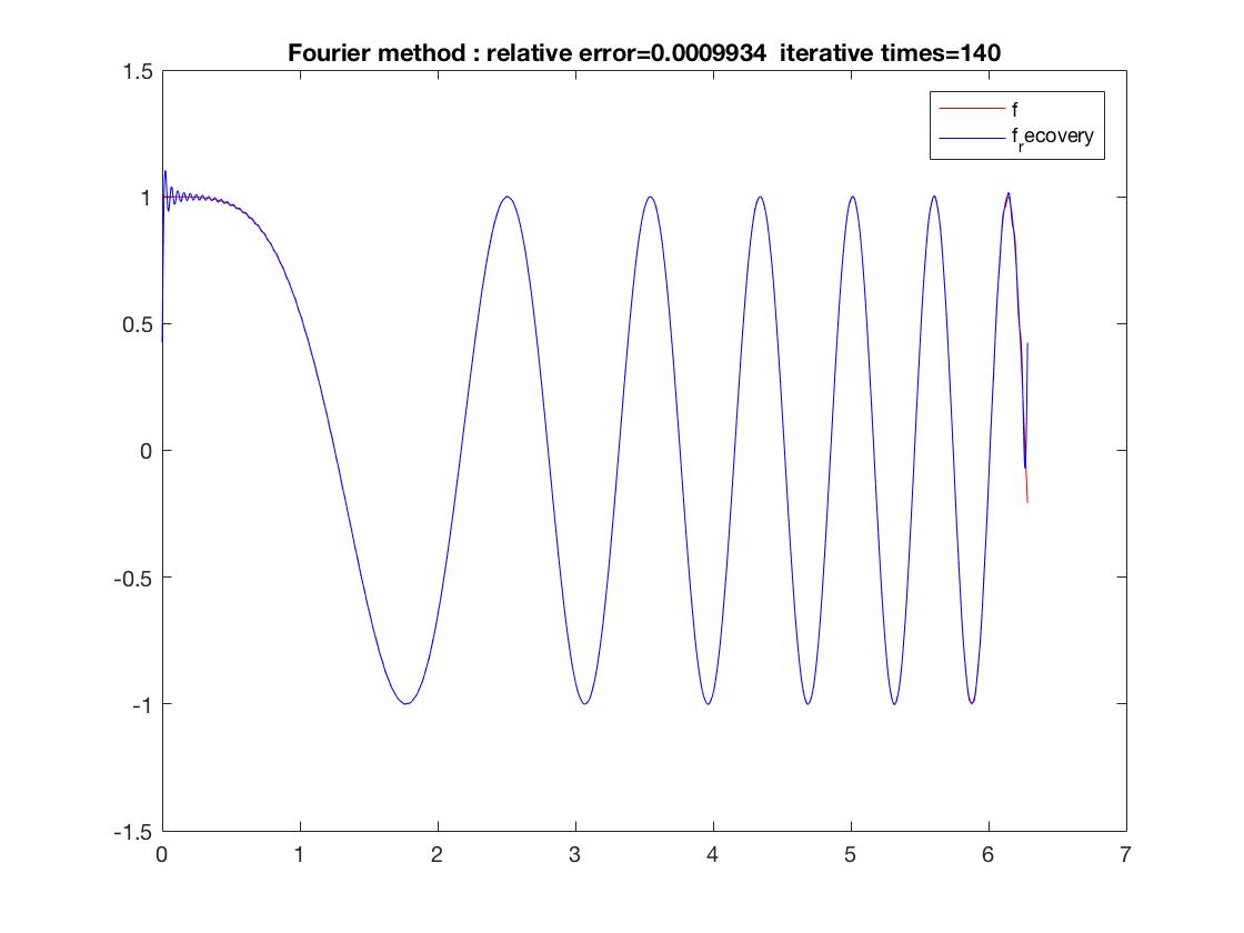
9 Experiments

Example 9.1

Fourier series and POAFD expansion is used to treat the chirp signal f​(t)=cos⁑t2.𝑓𝑑superscript𝑑2f(t)=\cos t^{2}. The results show that to reach the comparable errors Fourier needs 140 while POAFD needs 32 iterations.

Refer to caption
Refer to caption
Figure 9.1
Refer to caption
Table 9.1
Example 9.2

The second set of experiments given by figure 9.2 is for recovering functions βˆ‘k=010zk(k+1)2superscriptsubscriptπ‘˜010superscriptπ‘§π‘˜superscriptπ‘˜12\sum_{k=0}^{10}\frac{z^{k}}{(k+1)^{2}} and ∏k=110zβˆ’ak1βˆ’aΒ―k​z,superscriptsubscriptproductπ‘˜110𝑧subscriptπ‘Žπ‘˜1subscriptΒ―π‘Žπ‘˜π‘§\prod_{k=1}^{10}\frac{z-a_{k}}{1-\overline{a}_{k}z}, where aksubscriptπ‘Žπ‘˜a_{k} is randomly selected in 𝐃.𝐃\bf D. The results of 5 iterations are given by figure 9.2. By using the same iteration numbers, POAFD gives smaller relative error than Fourier, 1Γ—10βˆ’31superscript1031\times 10^{-3} and 8Γ—10βˆ’6,8superscript1068\times 10^{-6}, respectively. We also give comparison between different iteration numbers in figure 9.2 with respect to the same relative error. It shows that the iteration number of POAFD is ten iterations less than that of the Fourier method, being more efficient than the latter. The experiments show that for those examples POAFD outperforms Fourier.

Refer to caption
Refer to caption
Refer to caption
Refer to caption
Figure 9.2
Refer to caption
Table 9.2
Example 9.3

The third set of experiments given by figure 9.3 is for recovering a signal with a singular inner function part

1+2​z2(zβˆ’2)​(zβˆ’3)βˆ’1(z+2)​(z+3)​ez+1+z+izβˆ’i+zβˆ’iz+i.12superscript𝑧2𝑧2𝑧31𝑧2𝑧3superscript𝑒𝑧1𝑧𝑖𝑧𝑖𝑧𝑖𝑧𝑖\frac{1+2z^{2}}{(z-2)(z-3)}-\frac{1}{(z+2)(z+3)}e^{z+1+\frac{z+i}{z-i}+\frac{z-i}{z+i}}.

Under the same iteration number 150, we have higher convergence speed with smaller error than the Fourier method. It is seen in this example that by POAFD the high oscillatory parts are accurately approximated.

Refer to caption
Refer to caption
Figure 9.3
Refer to caption
Table 9.3
Example 9.4

In this experiment we can summarize from below the enclosed table that for functions of the reproducing kernel type, 1(1βˆ’a¯​z)2+Ξ²,a1superscript1Β―π‘Žπ‘§2π›½π‘Ž\frac{1}{(1-\overline{a}z)^{2+\beta}},a is close to βˆ‚πƒ,𝐃\partial\bf D, the POAFD in 𝔸β2subscriptsuperscript𝔸2𝛽\mathbb{A}^{2}_{\beta} performs with the best effect; and when α𝛼\alpha leaves away from β𝛽\beta the effectiveness of the POAFD in 𝔸β2subscriptsuperscript𝔸2𝛽\mathbb{A}^{2}_{\beta} for approximating 1(1βˆ’a¯​z)2+Ξ²1superscript1Β―π‘Žπ‘§2𝛽\frac{1}{(1-\overline{a}z)^{2+\beta}} is reduced (IN stands for iteration number, RE for relative error).

Refer to caption
Table 9.4

10 Conclusion

The validity of POAFD for the Bergman and weighted Bergman spaces in the unit disc and the upper-half complex plane contexts are evidenced through proving the right boundary vanishing properties or, alternatively, maximal selection theorems. The corresponding algorithms are established. We show that to gain the best approximation at every iterative step occasions of multiple selections of parameters are unavoidable. The process of repeating selection of parameters necessarily induces directional derivatives along with the G-S orthonormalization process. The orthonormal rational systems or weighted Bergman-TM-systems are constructed. The underlying study, in particular, promotes the topic rational approximation to holomorphic functions without boundary limits, and, in particular, with a variety of singularities at the boundary. The effectiveness and efficiency of the algorithms are tested through different types of Bergman space functions.

References

  • [1] Baratchart, L., Mai, W. X., Qian, T. (2016). Greedy algorithms and rational approximation in one and several variables. In Modern Trends in Hypercomplex Analysis (pp. 19-33).
  • [2] Bomash, G. (1992). A Blaschke-type product and random zero sets for Bergman spaces. Arkiv fΓΆr Matematik, 30(1), 45-60.
  • [3] Coifman R, Steinerberger S.(2017). Nonlinear phase unwinding of functions. J Fourier Anal Appl, 2017, 23: 778 V809.
  • [4] Coifman, R. R., Steinerberger, S., Wu, H. T. (2017). Carrier Frequencies, Holomorphy, and Unwinding. SIAM Journal on Mathematical Analysis, 49(6), 4838-4864.
  • [5] CUI Xue-wei, YANG Xue-mei(2000). Reproducing kernel of Bergman space on the upper half plane. Pure and Applied Mathematics. 2, 69-73.
  • [6] Duren, P. L., Schuster, A. (2004). Bergman spaces (No. 100). American Mathematical Soc..
  • [7] Elliott, S. J., Wynn, A. (2011). Composition operators on weighted Bergman spaces of a half-plane. Proceedings of the Edinburgh Mathematical Society, 54(2), 373-379.
  • [8] Hedenmalm, H., Korenblum, B., Zhu, K. (2012). Theory of Bergman spaces (Vol. 199). Springer Science and Business Media.
  • [9] Horowitz, C. (1994). Some conditions on Bergman space zero sets. Journal d’nalyse Mathematique, 62(1), 323-348.
  • [10] LeBlanc, E. (1990). A probabilistic zero set condition for the Bergman space. The Michigan Mathematical Journal, 37(3), 427-438.
  • [11] Mai, W., Qian, T. (2017). Aveiro method in reproducing kernel Hilbert spaces under complete dictionary. Mathematical Methods in the Applied Sciences, 40(18), 7240-7254.
  • [12] Mai, W., Qian, T. (2016). Rational approximation of functions in the hardy spaces on tubes. arXiv preprint arXiv:1604.07597.
  • [13] Mi, W., Qian, T. (2012). Frequency-domain identification: An algorithm based on an adaptive rational orthogonal system. Automatica, 48(6), 1154-1162.
  • [14] Mi, W., Qian, T. (2014). On backward shift algorithm for estimating poles of systems. Automatica, 50(6), 1603-1610.
  • [15] Nowak, M., Waniurski, P. (2003, March). Random zero sets for Bergman spaces. In Mathematical Proceedings of the Cambridge Philosophical Society (Vol. 134, No. 2, pp. 337-345). Cambridge University Press.
  • [16] Qian, T. (2016). Two-dimensional adaptive Fourier decomposition. Mathematical Methods in the Applied Sciences, 39(10), 2431-2448.
  • [17] T. Qian, Yanbo Wang(2011), Adaptive Fourier Series-A Variation of Greedy Algorithm, Advances in Computational Mathematics, 34(2011), no.3, 279-293.
  • [18] T. Qian, Y. B. Wang(2013), Remarks on Adaptive Fourier Decomposition, International Journal of Wavelets, Multiresolution and Information Processing, 2013, 11(1): 1-14.
  • [19] T. Qian(2015), Adaptive Fourier Transform, the Chinese Science Press (in Chinese).
  • [20] Wang, J., Qian, T. (2014). Approximation of monogenic functions by higher order SzegoΒ¨Β¨π‘œ\ddot{o} kernels on the unit ball and half space. Science China Mathematics, 57(9), 1785-1797.
  • [21] Zhu, K. (1997). Interpolating and recapturating in reproducing Hilbert Spaces. Bull. Hong Kong Math. Soc, 1, 21-33.