Constrained Optimal Consensus in Dynamical Networks

Abstract

In this paper, an optimal consensus problem with local inequality constraints is studied for a network of single-integrator agents. The goal is that a group of single-integrator agents rendezvous at the optimal point of the sum of local convex objective functions. The local objective functions are only available to the corresponding agents that only need to know their relative distances from their neighbors in order to seek the final optimal point. This point is supposed to be confined by some local inequality constraints. To tackle this problem, we integrate the primal-dual gradient-based optimization algorithm with a consensus protocol to drive the agents toward the agreed point that satisfies KKT conditions. The asymptotic convergence of the solution of the optimization problem is proven with the help of LaSalle’s invariance principle for hybrid systems. A numerical example is presented to show the effectiveness of our protocol.

1 Introduction

Over the last decade, cooperative control in a network of autonomous agents have been considered in scientific communities by virtue of big breakthroughs in wireless communication technology. Among these problems, consensus in dynamical networks is a central problem that has been studied from many aspects ren2007distributed ; cheng2016reaching ; fan2014semi ; rezaee2015average . In particular, the problem of optimal consensus among networked agents has recently gained considerable attention. In this setup, the final consensus value is required to minimize the sum of individual uncoupled convex functions. For instance, the paper rahili2015distributed resolved the optimal consensus problem over a network of single-integrator agents with time-varying objective function under the confining condition that Hessians associated with all local convex functions being identical. Later, they suggested a more sophisticated algorithm to relax this restriction. The authors of xie2017global proposed a bounded control law applied to a network of single-integrator agents to resolve the similar problem. In these works, agents admit no constraint. The optimal consensus problem can be formulated as distributed optimization problem nedic2010constrained ; lin2014constrained ; lu2012zero . In this setup, all interconnected agents cooperate with each other to seek the global optimal solution in a cooperative manner. Each agent minimizes its local cost function and exchanges its states’ information with its neighbors so that the team achieves the global optimum solution. In nedic2010constrained , a consensus protocol is integrated with a projection operator to reach an agreed point that is limited to the intersection of local constraint sets to solve a distributed constrained optimization problem. The article lin2014constrained extended the work by nedic2010constrained to study the problem of constrained consensus in unbalanced networks. The authors in lu2012zero presented a set of continuous-time algorithms called Zero-Gradient-Sum, by which the states of a whole network asymptotically converge to the solution to the associated unconstrained convex optimization problem along an invariant zero-gradient-sum manifold.
To resolve distributed optimization problems with inequality/equality constraints, some researches were conducted based on primal-dual methods. For example, the reference yi2015distributed proposed a continuous-time dynamics for seeking the saddle point of the sum of agents’ local Lagrangians to solve a distributed optimization problem with both inequality and equality constraints per node. The research paper yang2016multi presented a continuous-time protocol for distributed optimization problems with general constraints, relaxing the assumption of global convexity on each local objective function to convexity of locally bounded feasible region. In the both above-mentioned works, to attain consensus on the globally optimal solution, a Lagrangian multiplier is assigned to each agent for accommodating to consensus equality constraints. Then, all agents exchange the information of their Lagrangian multipliers (dual states) as well as the primal decision variables with their neighbors in order to reach consensus on the optimal solution. The papers wang2011control ; gharesifard2014distributed ; niederlander2016distributed exploited the same technique to fulfill consensus over networks.
In particular, in this paper, a novel solution to optimal consensus problems over undirected networks of single-integrator agents is presented. Such solution must also satisfy local convex inequalities for all agents. To tackle this problem, we split it into two parts, namely, a consensus sub-problem and an optimization one. Following this segmentation, we then propose a distributed continuous-time solution that consists of two parts: the first part yields the optimal points associated with local cost functions, and, at the same time, the second part drives the agents toward reaching consensus. In the proposed algorithm, each agent only needs to know its relative distances from its neighbors as well as its own objective function and constraint information. It is worthwhile noting that in applications such as swarm robots, the relative positions with their neighbors might be the only information that agents can have access to for constructing proper control actions. Our proposed algorithm makes the communication establishment, which is essential in the literature for exchanging the information of Lagrangian multipliers for reaching optimal consensus value, redundant and unnecessary. Besides, by the present approach less communication burdens are imposed on the agents in communication-based control setups. To establish the proposed algorithm, we present the stability analysis associated with perturbed dynamical systems and introduce a novel convergence proof with the help of LaSalle’s invariance principle for hybrid systems.
The results of the current paper provides further developments compared to the existing literature in this area.
i) Compared to wang2011control ; gharesifard2014distributed ; yang2016multi , in the present approach the agents do not need to exchange the information of their dual variables and can reach optimal consensus by only knowing their relative positions with respect to their neighbors.
ii) From design perspective, the penalty-based protocol studied in wang2011control ; gharesifard2014distributed ; kia2015distributed ; yi2015distributed ; yang2016multi ; niederlander2016distributed only admits linear consensus paradigm. This restricts the protocol illustrated in these references from adopting nonlinear consensus strategies that can in turn deliver fast convergence outcomes, see e.g. rahili2015distributed . Besides, in the case of high order dynamics, this approach does not work, see e.g. rahili2015distributed ; xie2017global . The algorithm introduced here does not have such limitation.
iii) Even though the problem studied here is closely related to that of in rahili2015distributed ; xie2017global ; lu2012zero ; kia2015distributed , unlike the current paper, these references only addressed unconstrained optimization.
iv) While the references nedic2010constrained ; lin2014constrained explored constrained optimization problems with convex set constraints, the projection operator utilized therein is difficult to handle in real-time specially when a large number of constraints are involved. Since a closed convex set can be approximated by a polyhedron set that is constituted by a set of linear equalities and inequalities, one can cast the optimization problem of nedic2010constrained ; lin2014constrained into the present formulation and adopt an easy-to-handle gradient-based primal-dual method discussed here to resolve it.
v) The proposed algorithm achieves a less perplexed states’s trajectories toward the final point compared to the existing penalty-based algorithms (see Section 4).
This paper is organized as follows. The problem formulation is given Section 2. Then, our proposed solution is presented in Section 3. A numerical example is presented in Section 4. Finally, the concluding remarks and suggestions for future studies are given in Section 5.

2 Problem Formulation

Consider $N$ physical agents over a network with time-invariant undirected graph $\mathcal{G}=(\mathcal{N},E,A)$, where $\mathcal{N}=\{1,\ldots,N\}$ is the node set, $E\subseteq\mathcal{N}\times\mathcal{N}$ is the edge set , and $A=[a_{ij}]$ is a weighted adjacency matrix. Each pair $e=(i,j)\in E$ indicates link between the node $i$ and the node $j$ in an undirected graph. Suppose that each agent is described by the continuous-time single-integrator dynamics

$${\dot{x}_{i}}(t)={u_{i}}(t),\quad$$ (1)

where $x_{i}(t)\in\mathbb{R}$ represents the position of agent $i$, and $u_{i}(t)$ is the control input to agent $i$. We shall drop the argument $t$ throughout this paper unless it is necessary. It is worhwhile noting that here we consider only one dimensional agents for the sake of simplicity in notations. However, it is straightforward to show that our algorithm can be extended to higher dimensional dynamics as each dimension is decoupled from others and can be treated independently. The agents are supposed to reach at an agreed point that shall minimize a convex optimization problem as

$$\begin{split}\min\,f(x)=\sum_{i=1}^{N}f_{i}(x)\\ \text{subject to}\,g_{i}(x)\leq 0,\end{split}$$ (2)

in which $f_{i}(\cdot):\mathbb{R\rightarrow\mathbb{R}}$ is the local cost function associated with node $i$ in the network. Furthermore, $g_{i}(\cdot):\mathbb{R\rightarrow\mathbb{R}}$ represents a constraint on the optimal position and is associated with node $i$. It is supposed that each agent knows only its associated cost function and inequality constraint function. We assumed only one inequality constraint per node for complexity avoidance; our algorithm can solve the same problem with a desired number of inequality constraints.

We consider the following assumptions in relation to the problem (2).
Assumption 1.

1. The objective functions $f_{i}(\cdot)$, $i\in\mathcal{N}$ , and $g_{i}(\cdot)$, $i\in\mathcal{N}$, are convex and continuously differentiable on $\mathbb{R}$.

2. The aggregate cost function $\sum_{i=1}^{N}f_{i}(\cdot)$ is radially unbounded on $\mathbb{R}$.

Assumption 2. (Slater’s Condition) There exists $x^{*}\in\mathbb{R}$ such that $g_{i}(x^{*})\leq 0$.

The Assumption 1 and 2 fulfill the solution existence conditions for the optimization problem (2). Note that the constrained optimal consensus problem that was defined above is equivalent with the following distributed convex optimization problem

$$\begin{array}[]{cc}\underset{\underset{i=1,\cdots,N}{x_{i}}}{\text{min}}\sum_{i=1}^{N}f_{i}(x_{i})\\ \text{subject to}\,x_{i}=x_{j}\,\text{and}\,g_{i}(x_{i})\leq 0,\end{array}$$ (3)

In the problem (3), the consensus constraint, i.e. $x_{i}=x_{j},$ $i,j=1,\ldots,N$, is imposed to guarantee the same decision variable is achieved eventually. Here, the agents with dynamics as in (1) shall seek the optimal point $x^{*}$ i.e. $x_{i}=x^{*}$, $i\in\mathcal{N}$, which minimize the collective cost function $\sum_{i=1}^{N}f_{i}(x_{i})$ in a distributed fashion, given inequality constraints $g_{i}(x_{i})\leq 0$, $i\in\mathcal{N}$. To this end, each agent searches for the minimum of its associated cost function, $f_{i}(x_{i})$, with regards to its local inequality constraint, $g_{i}(x_{i})$, not knowing other local cost functions and constraint inequalities. Furthermore, all agents shall reach an agreement on their positions through only knowing the relative distances from their neighboring agents. Now, we shall design the control input $u_{i}$ to fulfill these requirements.

One can say that the problem (3) consists of a minimization sub-problem, with inequality constraints, and a consensus sub-problem. This splitting is the cornerstone of our approach to resolve the problem (2). The minimization sub-problem can be defined as

$$\begin{split}\underset{\underset{i=1,\cdots,N}{x_{i}}}{\min}\sum_{i=1}^{N}f_{i}(x_{i})\\ \text{subject to}\,g_{i}(x_{i})\leq 0,\end{split}$$ (4)

and the consensus sub-problem is

$$\underset{t\rightarrow\infty}{\text{lim}}\,(x_{i}-x_{j})=0,\,\,\,\,i,j=1,\ldots,N.$$ (5)

Before proceeding to solving the above mentioned sub-problems, i.e. the minimization sub-problem (4) and the consensus sub-problem (5), we present some optimality conditions for the optimization sub-problem through the following lemma. Later in Section 3, we will use these conditions to show the convergence of our algorithm.

Lemma 1

(boyd2004convex, , p. 243) (KKT Conditions) Given Assumption 1 and 2, $\overline{x}^{*}=\left[x_{1}\ldots x_{N}\right]^{\top}$ is the optimal solution of the problem (4) if and only if there exist Lagrangian multipliers, $\lambda_{i}^{*}>0$ , $i=1,\ldots,N$, such that the following conditions are satisfied

$$g_{i}(x_{i}^{*})\leq 0,\,\,\,\,\,\,\lambda_{i}^{*}g_{i}(x_{i}^{*})=0,\,\,\,\,\,i=1,\ldots,N,$$ (6)

$$\sum_{i}^{N}\frac{\partial f_{i}(x_{i}^{*})}{\partial x_{i}}+\lambda_{i}^{*}\frac{\partial g_{i}(x_{i}^{*})}{\partial x_{i}}=0,\,\,\,\,i=1,\ldots,N.$$ (7)

To solve the minimization sub-problem (4), we focus on the primal-dual method that seeks the saddle point of the Lagrangian associated with convex optimization sub-problem (4). The Lagrangian is defined by

$$L(\bar{x},\bar{\lambda})=\sum_{i=1}^{N}f_{i}(x_{i})+\lambda_{i}g_{i}(x_{i}),$$ (8)

where $\bar{\lambda}=\left[\lambda_{1}\ldots\lambda_{N}\right]^{\top}$and $\bar{x}=\left[x_{1}\ldots x_{N}\right]^{\top}$. $L(\bar{x},\bar{\lambda})$ is convex in $\bar{x}$ and concave in $\bar{\lambda}$. We have the following properties for $L(\bar{x},\bar{\lambda})$,

$$L(\bar{x}^{*},\bar{\lambda}) \geq L(\bar{x},\bar{\lambda})+\nabla_{\bar{x}}L(\bar{x},\bar{\lambda})^{\top}.(\bar{x}^{*}-\bar{x}),$$ (9)

$$L(\bar{x},\bar{\lambda}^{*}) \leq L(\bar{x},\bar{\lambda})+\nabla_{\bar{\lambda}}L(\bar{x},\bar{\lambda})^{\top}.(\bar{\lambda}^{*}-\bar{\lambda}),$$ (10)

where $\left(\bar{x}^{*},\bar{\lambda}^{*}\right)$ is said to be the saddle point of $L(\bar{x},\bar{\lambda})$ (boyd2004convex, , p. 238). The following inequalities hold for all $(\bar{x},\bar{\lambda})\in dom(L)$

$$L(\bar{x}^{*},\bar{\lambda})\leq L(\bar{x}^{*},\bar{\lambda}^{*})\leq L(\bar{x},\bar{\lambda}^{*}).$$ (11)

From (8), one can define the Lagrangian function for node $i$ as

$$L_{i}(x_{i},\lambda_{i})=f_{i}(x_{i})+\lambda_{i}g_{i}(x_{i}).$$ (12)

In the sequel, we will use $L$ and $L_{i}$ to denote the aggregate Lagrangian (8) and the Lagrangian corresponding to node $i$, i.e. (12), respectively. Hence, the main task of this paper is to find the saddle point of (8) while consensus on the agents’ states is also achieved.

3 Main Results

We propose the following algorithm to find the saddle point of (8) and satisfy the consensus constraint (5)

$$\dot{x}_{i} = -\alpha\nabla_{x_{i}}L_{i}+h_{i},\,\,\,\,\,\,\,i=1,\ldots,N,$$ (13)

$$\dot{\lambda}_{i} = \left[\nabla_{\lambda_{i}}L_{i}\right]_{\lambda_{i}}^{+},$$ (14)

where $\alpha>0$ and $h_{i}=-\beta\sum_{j\in\mathcal{N}_{i}}(x_{i}-x_{j})$ with $\beta>0$. $\mathcal{N}_{i}=\{j|j\in\mathcal{N},(j,i)\in E\}$ is the set of neighbors corresponding to node $i$. Note that $-\alpha\nabla_{x_{i}}L_{i}+h_{i}$ acts as the control input for agent $i$, i.e.

$$u_{i}=-\alpha\nabla_{x_{i}}L_{i}+h_{i}.$$ (15)

In (14), a positive projection is used to ensure that Lagrangian multipliers remain non-negative. For scalars, $\left[p\right]_{q}^{+}=p$ if $p>0$ or $q>0$, and $\left[p\right]_{q}^{+}=0$ otherwise. When $\left[p\right]_{q}^{+}=0$, the projection is said to be active. Therefore, in (14) when $\lambda_{i}>0$ and $g_{i}(x_{i})<0$, $\dot{\lambda}_{i}<0$ and $\lambda_{i}$ decreases until it reaches $0$ where the projection becomes active and it remains $0$ until the sign of $g_{i}(x_{i})$ turns. Note that we start with $\lambda_{i}(0)>0$; therefore, $\lambda_{i}\geq 0$ for all $t>0$. One can define the set of active projection by $\sigma=\{i:\lambda_{i}=0,\,g_{i}(x_{i})<0\}$. Note that the control command (15), consists of two parts. The first part is to minimize the local cost function and the second part is associated with the consensus error. The following lemma is instrumental to some of the results presented in this paper.

Lemma 2

horn2012matrix (Courant-Fischer Formula) The second smallest non-zero eigenvalue of the matrix $M\in\mathbb{R}^{N\times{N}}$, that we denote by $v_{2}(M)$, satisfies $v_{2}(M)=\displaystyle\min_{x^{\top}\mathbf{1}_{N}=0,x\neq\mathbf{0}_{N}}\frac{x^{\top}Mx}{x^{\top}x}$.

Before proving that the algorithm in (13) and (14) yields the saddle point of (8), we show that the positions of agents, $x_{i}$, $i\in\mathcal{N}$, reach consensus, when taking control input as $u_{i}=-\alpha\nabla_{x_{i}}L_{i}+h_{i}$, $i\in\mathcal{N}$. This is established in the next proposition.

Proposition 1

Suppose that the graph $\mathcal{{G}}$ is connected and undirected. Then, there exists some finite $t_{1}$ such that the agents (1) satisfy $\left|x_{i}(t)-x_{j}(t)\right|\leq\delta_{0}$, $i,j=1,\ldots,N$, with $\delta_{0}$ small as desired, for $t>t_{1}$ (15), if $\left|\nabla_{x_{i}}L_{i}-\nabla_{x_{j}}L_{j}\right|<\omega_{0}$, $i,j=1,\ldots,N$, with $\omega_{0}\in{\mathbb{R}}^{+}$.

Proof

The aggregate dynamics of agents (1) with (15) is $\dot{\bar{x}}=-\beta DD^{\top}\bar{x}+\Omega,$ where $\varOmega=[-\alpha\nabla_{x_{1}}L_{1}\ldots-\alpha\nabla_{x_{N}}L_{N}]^{\top}$. Let the network’s consensus error be defined by $\bar{e}_{x}=\Pi\bar{x}$, where $\Pi=I_{N}-\frac{1}{N}\mathbf{1}_{N}\mathbf{1}_{N}^{\top}$ and $\bar{x}$ denotes the aggregate state of the network, that is defined by $\bar{x}=\left[x_{1}\ldots x_{N}\right]^{\top}$. Note that $\mathbf{1}^{\top}\Pi=\mathbf{0}$ and $\Pi\mathbf{1=0}$. Thus, one can write

$$\dot{\bar{e}}_{x}=-\beta DD^{\top}\bar{e}_{x}+\Pi\Omega,$$ (16)

where $D=[d_{ik}]\in\mathbb{R}^{N\times|E|}$ is the incidence matrix associated with the topology $\mathcal{G}$. And, its entries i.e. $d_{ik}$, are obtained by assigning an arbitrary orientation for the edges in $\mathcal{G}$. For instance, if one considers the $k^{th}$ edge i.e. $e_{k}=(i,j)$, then $d_{ik}=-1$ if the edge $e_{k}$ leaves node $i$, $d_{ik}=1$ if it enters node $i$, and $d_{ik}=0$ otherwise. We choose the Lyapunov candidate function $V(\bar{e}_{x})=\frac{1}{2}\bar{e}_{x}^{\top}\bar{e}_{x}$. By taking time derivative from $V(\bar{e}_{x})$ along the trajectories of $\bar{e}_{x}$, one can write

$$\dot{V}(\bar{e}_{x}) = -\beta\bar{e}_{x}^{T}DD^{\top}\bar{e}_{x}+\bar{e}_{x}^{\top}\Pi\Omega$$ (17)

$$\leq -\beta{v}_{2}(DD^{\top})\left\|\bar{e}_{x}\right\|^{2}+\bar{e}_{x}^{\top}\Pi\Omega$$

$$\leq -\beta{v}_{2}(DD^{\top})\left\|\bar{e}_{x}\right\|^{2}+\alpha\left\|\bar{e}_{x}\right\|\omega_{0}$$

where ${v}_{2}({DD^{\top}})$ denotes the smallest non-zero eigenvalue of $DD^{\top}$. In the above, the first inequality is resulted from Lemma 2, and the second inequality is resulted from the assumption $\left|\nabla_{x_{i}}L_{i}-\nabla_{x_{j}}L_{j}\right|<\omega_{0}$ given in the statement of the proposition. From (17), one can say that

$$\dot{V}(\bar{e}_{x})\leq-\theta\left\|\bar{e}_{x}\right\|^{2}+\left(\left(\theta-\beta{v}_{2}(DD^{\top})\right)\left\|\bar{e}_{x}\right\|+\alpha\omega_{0}\right)\left\|\bar{e}_{x}\right\|,$$ (18)

where $0<\theta<1$. For $\left\|\bar{e}_{x}\right\|\geq\displaystyle\frac{\omega_{0}\alpha}{\beta{v}_{2}(DD^{\top})\theta}$, we obtain $\dot{V}(\bar{e}_{x})<0$. Now, we are ready to invoke Theorem 5.1 from khalil1996nonlinear that guarantees that by choosing $\beta$ large enough, one can make the consensus error, $\delta_{0}$, as small as desired.

Remark 1

Assumption $\left|\nabla_{x_{i}}L_{i}-\nabla_{x_{j}}L_{j}\right|<\omega_{0}$ in Proposition 1 seems to be unreasonable at the first glance as it assumes that the primal and dual variables $x_{i}$ and $\lambda_{i}$, $i=1,\ldots,N$, must remain bounded. However, we will show by the following lemma that this requirement always holds. It is worthwhile mentioning that by choosing a conservative bound on $\omega_{0}$ one can adjust the protocol’s parameters to reach consensus with any desired accuracy.

We now assert that the trajectories generated by the dynamics (13) and (14) are globally bounded.

Lemma 3

Given that the graph $\mathcal{G}$ is connected and undirected, the solutions of (13) and (14) are globally bounded.

Proof

We study boundedness of the solutions of (13) and (14) by Lyapunov stability analysis. Let us define a quadratic Lyapunov function as

$$W(\bar{x},\bar{\lambda})=\frac{1}{2\alpha}(\bar{x}-\bar{x}^{*})^{\top}(\bar{x}-\bar{x}^{*})+\frac{1}{2}(\bar{\lambda}-\bar{\lambda}^{*})^{\top}(\bar{\lambda}-\bar{\lambda}^{*}).$$ (19)

In the above equation, $\left(\bar{x}^{*},\bar{\lambda}^{*}\right)$ represents a saddle point equilibrium associated with $L(\bar{x},\bar{\lambda})$. By taking derivative from both sides of (19) along the trajectories (13) and (14), with respect to time, we will have

$$\dot{W}(\bar{x},\bar{\lambda}) = -(\bar{x}-\bar{x}^{*})^{\top}\mathbf{\mathbf{\nabla}}_{\bar{x}}L+\frac{1}{\alpha}(\bar{x}-\bar{x}^{*})^{\top}H$$ (20)

$$+\sum_{i=1}^{N}(\lambda_{i}-\lambda_{i}^{*})\left[\nabla_{\lambda_{i}}L_{i}\right]_{\lambda_{i}}^{+},$$

where $\mathbf{\mathbf{\nabla}}_{\bar{x}}L=\left[\nabla_{x_{1}}L_{1}\ldots\nabla_{x_{N}}L_{N}\right]^{\top}$ and $H=\left[h_{1}\ldots h_{N}\right]^{\top}$.

Suppose that for some index $i$, the projection becomes active i.e. $i\in\sigma$. In this case $\lambda_{i}=0$ and $\nabla_{\lambda_{i}}L_{i}=g_{i}(x_{i})<0$. It is worthwhile noting that $\lambda_{i}<0$ never holds when parameters are initialized by positive values. Thus, in this case one can conclude that $(\lambda_{i}-\lambda_{i}^{*})\nabla_{\lambda_{i}}L_{i}\geq 0$ due to the fact that $\nabla_{\lambda_{i}}L_{i}<0$ and $\lambda_{i}^{*}\geq 0$. On the other hand, for the agents the projection is not active, $(\lambda_{i}-\lambda_{i}^{*})\left[\nabla_{\lambda_{i}}L_{i}\right]_{\lambda_{i}}^{+}=$ $(\lambda_{i}-\lambda_{i}^{*})\nabla_{\lambda_{i}}L_{i}$ holds. Thus, we can assert that the following inequality holds.

$$\dot{W}(\bar{x},\bar{\lambda})\leq-(\bar{x}-\bar{x}^{*})^{\top}\mathbf{\mathbf{\nabla}}_{\bar{x}}L+\frac{1}{\alpha}(\bar{x}-\bar{x}^{*})^{\top}H+(\bar{\lambda}-\bar{\lambda}^{*})^{\top}\nabla_{\bar{\lambda}}L.$$ (21)

Then, from (9) and (10), we have

$$\dot{W}(\bar{x},\bar{\lambda}) \leq-L(\bar{x}^{*},\bar{\lambda})+L(\bar{x},\bar{\lambda})+\frac{1}{\alpha}(\bar{x}-\bar{x}^{*})^{\top}H$$

$$-L(\bar{x},\bar{\lambda})+L(\bar{x},\bar{\lambda}^{*})$$

$$\leq\frac{1}{\alpha}(\bar{x}-\bar{x}^{*})^{\top}H$$ (22)

$$=-\frac{\beta}{\alpha}\sum_{i=1}^{N}(x_{i}-x^{*})\sum_{j\in{N}_{i}}(x_{i}-x_{j})$$

$$=-\frac{\beta}{\alpha}\sum_{i=1}^{N}x_{i}\sum_{j\in\mathcal{N}_{i}}(x_{i}-x_{j}).$$ (23)

The inequality (22) is due to (11). Furthermore, the last equality results from the fact that $\sum_{i=1}^{N}\sum_{j\in\mathcal{N}_{i}}(x_{i}-x_{j})=0$ in a network with the undirected graph $\mathcal{{G}}$. It is easy to show that $-\sum_{i=1}^{N}x_{i}\sum_{j\in\mathcal{N}_{i}}(x_{i}-x_{j})\leq 0$ in an undirected graph. Hence, $\dot{W}(\bar{x},\bar{\lambda})\leq 0$, and, thus, the proof is concluded.

The dynamics (13) and (14) can be regarded as a hybrid system due to switching projection operator on the right side of the relation (14). Thus, before proceeding to the main result of this section, we introduce the LaSalle’s invariance principle for hybrid systems through a lemma first given in lygeros2003dynamical and later summarized in feijer2010stability .

Lemma 4

feijer2010stability Consider the hybrid dynamics (13) and (14) with a compact invariant set $\mathcal{O}$ and there exists a continuously differentiable positive function ${V}(\dot{\bar{x}},\dot{\bar{\lambda}};\sigma)$ that decreases along trajectories in $\mathcal{O}$. Then, every trajectory generated by the hybrid dynamics and initiated in $\mathcal{O}$ converges to $M$, the maximal invariant set within $\mathcal{O}$, which satisfies

• $\dot{V}(\dot{\bar{x}},\dot{\bar{\lambda}};\sigma)=0$ in intervals of fixed $\sigma$,

• $V(\dot{\bar{x}},\dot{\bar{\lambda}};\sigma^{-})=V(\dot{\bar{x}},\dot{\bar{\lambda}};\sigma^{+})$ if $\sigma$ switches between $\sigma^{-}$and $\sigma^{+}$.

Next, in the light of the above lemma, we express the main result of this section.

Theorem 3.1

Assume that $f_{i}(x_{i})$ and $g_{i}(x_{i})$, $i\in\mathcal{N}$, are twice continuously differentiable on $\mathbb{R}$. Given Assumption 1 and 2, the dynamics (13) and (14) will converge to $\left(\bar{x}^{*},\bar{\lambda}^{*}\right)$ that is the solution to the optimization sub-problem (4).

Proof

To prove the theorem, it suffices to show that dynamics (13) and (14) will converge to a saddle point associated with the Lagrangian function (8). To this end, we split the proof into two parts. We first illustrate that the Lyapunov function

$$V(\dot{\bar{x}},\dot{\bar{\lambda}};\sigma)=\frac{1}{2\alpha}\sum_{i=1}^{N}\dot{x}_{i}^{2}+\frac{1}{2}\sum_{i=1,i\notin\sigma}^{N}\dot{\lambda}_{i}^{2}.$$ (24)

is always decreasing. Then, in the second part, we appeal to Lemma 4 to establish that the optimality conditions in Lemma 1 hold. To examine the above Lyapunov function, we only need to consider two scenarios, namely, the one in which the index set $\sigma$ changes and the other one where this set is fixed. One should note that in the former case the Lyapunov function (24) might be discontinuous as $\dot{\lambda}_{i}$ switches when $\sigma$ changes according to (14). However, in the latter, the Lyapunov function (24) is continuous. In the following, we establish that in both cases the positive function (24) is always non-increasing. We first assume that $\sigma$ is fixed. Taking derivative of $V(\dot{\bar{x}},\dot{\bar{\lambda}};\sigma)$ along the trajectories (13) and (14) with respect to time, we obtain

$$\begin{split}\dot{V}(\dot{\bar{x}},\dot{\bar{\lambda}};\sigma)=&\sum_{i=1}^{N}\dot{x}_{i}\left(-\frac{\partial^{2}L_{i}}{\partial x_{i}^{2}}\dot{x}_{i}-\frac{\partial^{2}L_{i}}{\partial\lambda_{i}\partial x_{i}}\dot{\lambda}_{i}+\frac{\dot{h}_{i}}{\alpha}\right)\\ &+\sum_{i=1,i\notin\sigma}^{N}g_{i}(x_{i})\frac{\partial g_{i}(x_{i})}{\partial x_{i}}\dot{x}_{i}\end{split}$$ (25)

The above equations can be simplified by expanding some of its terms into two cases, namely, $i\in\sigma$ and $i\notin\sigma$. Note that when $i\in\sigma$, $\lambda_{i}=0$, $\dot{\lambda}_{i}=0$. Thus, we can write

$$\dot{V}(\dot{\bar{x}},\dot{\bar{\lambda}};\sigma) =-\sum_{i=1}^{N}\dot{x}_{i}\left(\frac{\partial^{2}f_{i}(x_{i})}{\partial x_{i}^{2}}\dot{x}_{i}-\frac{\dot{h}_{i}}{\alpha}\right)$$

$$-\sum_{i=1,i\notin\sigma}^{N}\dot{x}_{i}\left(\lambda_{i}\frac{\partial^{2}g_{i}(x_{i})}{\partial x_{i}^{2}}\dot{x_{i}}+\frac{\partial g_{i}(x_{i})}{\partial x_{i}}g_{i}(x_{i})\right)$$

$$+\sum_{i=1,i\notin\sigma}^{N}g_{i}(x_{i})\frac{\partial g_{i}(x_{i})}{\partial x_{i}}\dot{x}_{i}.$$ (26)

Then after a simple algebraic simplification, it is easy to verify that

$$\dot{V}(\dot{\bar{x}},\dot{\bar{\lambda}};\sigma) = -\sum_{i=1}^{N}\dot{x}_{i}^{2}\frac{\partial^{2}f_{i}(x_{i})}{\partial x_{i}^{2}}-\sum_{i=1,i\notin\sigma}^{N}\lambda_{i}\dot{x}_{i}^{2}\frac{\partial^{2}g_{i}(x_{i})}{\partial x_{i}^{2}}$$ (27)

$$+\frac{1}{\alpha}\sum_{i=1}^{N}\dot{x}_{i}\dot{h}_{i}.$$

From the definition of $h_{i}$, we attain the following equality.

$$\sum_{i=1}^{N}\dot{x}_{i}\dot{h}_{i}=-\frac{\beta}{2}\sum_{i=1}^{N}\sum_{j\in\mathcal{N}_{i}}\left(\dot{x}_{i}-\dot{x}_{j}\right)^{2}.$$ (28)

Now, with substituting (28) in (27), we obtain

$$\dot{V}(\dot{\bar{x}},\dot{\bar{\lambda}};\sigma) = -\sum_{i=1}^{N}\dot{x}_{i}^{2}\frac{\partial^{2}f_{i}(x_{i})}{\partial x_{i}^{2}}-\sum_{i=1,i\notin\sigma}^{N}\lambda_{i}\dot{x}_{i}^{2}\frac{\partial^{2}g_{i}(x_{i})}{\partial x_{i}^{2}}$$ (29)

$$-\frac{\beta}{2\alpha}\sum_{i=1}^{N}\sum_{j\in\mathcal{N}_{i}}\left(\dot{x}_{i}-\dot{x}_{j}\right)^{2}$$

From Assumption 1 and that $\frac{\beta}{\alpha}>0$, it is attained that

$$\dot{V}(\dot{\bar{x}},\dot{\bar{\lambda}};\sigma)\leq 0.$$ (30)

Hence, ${V}(\dot{\bar{x}},\dot{\bar{\lambda}};\sigma)$ is non-increasing when $\sigma$ does not change.
In the following, we will show that the same property holds even when the set $\sigma$ changes. Consider conditions under which the index set $\sigma$ varies: (1) Consider the case at given time index, say $t_{0}$, the index set $\sigma$ is enlarged. This happens when there is a larger number of constraints with $g_{i}(x_{i}(t_{0}^{+}))<0$ compared to those with $g_{i}(x_{i}(t_{0}^{-}))<0$. We then obtain $V(t^{+})\leq V(t_{0}^{-})$ as $\dot{\lambda}_{i}(t_{0}^{+})=0$. Here $t_{0}^{-}$ and $t_{0}^{+}$ stand for the moment just before and after $t_{0}$, respectively. (2) Now suppose that the index set $\sigma$ shrinks. This case occurs when the set loses a constraint $i$ at time $t_{0}$ and $g_{i}(x_{i}(t_{0}^{+}))$ becomes positive. Since $g_{i}\left(\cdot\right)$ is a continuous function and $x_{i}$ is continuous as well, it can be said that this function has passed through zero to become positive. The latter supports that the new term ${\dot{\lambda}_{i}}^{2}$ is added to $V(\dot{\bar{x}},\dot{\bar{\lambda}};\sigma)$ but since $g_{i}(x_{i}(t_{0}^{+}))=g_{i}(x_{i}(t_{0}^{-}))$, no discontinuity happens. Therefore, one can say $V(\dot{\bar{x}},\dot{\bar{\lambda}};\sigma)$ does not change in this case and, therefore, remains non-increasing according to (30).
Now, we invoke Lemma 4 that presents LaSalle’s invariance principle for hybrid systems. From Lemma 3, we conclude that whole space $\mathbb{R}^{2N}$ represents an invariant set for the hybrid dynamics (13) and (14). On the other hand, in the first part of the proof, we showed that the Lyapunov function (24) decreases along the trajectories produced by (13) and (14). According to the statement of Lemma 4 there should exist maximal invariant set, say $M$, that satisfies conditions (a) and (b) stated in Lemma 4. In the sequel, we will show that (13) and (14) will stabilize at the point in which conditions (a) and (b) are met; moreover, the KKT conditions (6) and (7) are also fulfilled.

We first attend to part (a). From the equation (29), we attain $\dot{x}_{i}=0$, $i\in\mathcal{N}$, i.e. $\bar{x}\equiv\bar{x}^{*}$ since one can derive from (13) that $\bar{x}$ is continuous. Also, $\sum_{i=1}^{N}\dot{x}_{i}=-\alpha\sum_{i=1}^{N}\nabla_{x_{i}}L_{i}$. So, $\sum_{i=1}^{N}\nabla_{x_{i}}L_{i}=0$. Thereby, (7) is satisfied.

As for $\bar{\lambda}$, assume that $g_{i}(x_{i}^{*})>0$, then, $\lambda_{i}$ will grow unboundedly that it contradicts its boundedness shown earlier in Lemma 3. Therefore, $g_{i}(x_{i}^{*})\leq 0$, then two possible cases happen: i) $\lambda_{i}$ would decrease until it reaches at zero, producing a discontinuity once the projection becomes active. This would contradict with part (b) of Lemma 4. ii) $\lambda_{i}=0$; the corresponding projection is active for some $i$. Thus, $g_{i}(x_{i}^{*})\leq 0$ and $\lambda_{i}^{*}=0$ always hold, and, (6) is met.

In the above, we showed that the equilibrium point of the dynamics (13) and (14) is a saddle point of the Lagrangian function (8), and in the light of Saddle Point Theorem (ruszczynski2006nonlinear, , Theorem 4.7), it is the optimal solution to (4).

One should note that through Proposition 1, we showed consensus on states, i.e. $x_{i}=x_{j}$, $i,j=1,\ldots,N$. Furthermore, by Theorem 3.1, we proved that the control inputs (15) drive the agents towards the saddle point of the Lagrangian associated with (4). Hence, the optimal consensus problem (3) associated with the network of single-integrator agents (1) is resolved.

Remark 2

There exists a trade-off between size of the control command and permitted consensus error when selecting parameters $\alpha$ and $\beta$. As $\beta$ increases, according to Proposition 1, the consensus error becomes smaller while the control input size attains a larger value. On the other hand, with small $\alpha$, the consensus error decreases; however, this decelerates the optimization process.

4 Simulation Example

As mentioned earlier, results of the current paper also hold when agents are modeled by several integrators i.e. $x_{i}\in\mathbb{R}^{m}$. We exploit this fact and consider the following scenario that clearly exhibits the results of this paper through a numerical simulation. Consider four agents that move in a 2-D space and are connected under a ring topology. Assume that each agent is modeled by one single-integrator dynamics per coordinate. Their local objective functions are as $f_{1}(x_{11},x_{12})=x_{11}^{2}+x_{12}^{2},f_{2}(x_{21},x_{22})=(x_{21}-4)^{2}+(x_{22}-2)^{2},f_{3}(x_{31},x_{32})=(x_{31}-3)^{2}+4(x_{32}-1)^{2},f_{4}(x_{41},x_{42})=(x_{41}-1)^{2}$ Agent 1 has a local constraint as $g_{1}(x_{11},x_{12})=-x_{11}-x_{12}+1\leq 0$. Agent 2 suffers the constraint $g_{2}(x_{21},x_{22})=x_{21}^{2}+x_{22}^{2}-2\leq 0$. Agent 3 has the local constraint $g_{3}(x_{31},x_{32})=x_{31}^{2}+x_{32}^{2}-1\leq 0$, while agent 4 has no constraint. Let $\alpha=0.1$ and $\beta=10$ be the control law’s coefficients as in (15). Under the control law (15), the trajectories of agents’ positions are shown in Fig. 1 when the initial positions of the agents 1, 2, 3, and 4 are set as $x_{1}=\left[\begin{array}[]{cc}2&3\end{array}\right]^{\top}$, $x_{2}=\left[\begin{array}[]{cc}1&4\end{array}\right]^{\top}$, $x_{3}=\left[\begin{array}[]{cc}3&4\end{array}\right]^{\top}$, and $x_{4}=\left[\begin{array}[]{cc}5&0\end{array}\right]^{\top}$, respectively. We set the initial values for the Lagrangian multipliers as zero. The optimal solution to the problem is $\left[\begin{array}[]{cc}0.85&0.53\end{array}\right]^{\top}$.
Among many existing penalty-based algorithm , due to the page limitation, we only compare our result with that of the algorithm proposed by yi2015distributed on the above example (see Fig. 2). As it is observed, with the primal-dual dynamics proposed in yi2015distributed , the agents spiral around the optimal point in a perplexed way to reach the optimal point. Such trajectories towards the final point will impose too much energy consumption and practically are not feasible to achieve.

5 Conclusion

We studied constrained optimal consensus problem for an undirected network of single-integrator agents. We proposed a fusion algorithm in which: i) a primal-dual gradient method was used to satisfy KKT conditions for constrained convex optimization problems, and ii) a consensus protocol was adopted to make all agents reach the agreed optimal value. Then, through the theory of stability of perturbed systems, we showed that this algorithm delivers consensus. Moreover, we proved that the equilibrium point of the network’s dynamics coincides with the optimal solution to the optimization problem, adopting the LaSalle’s invariance principle for hybrid systems. Finally, we illustrated the performance of our proposed algorithm through a numerical example.

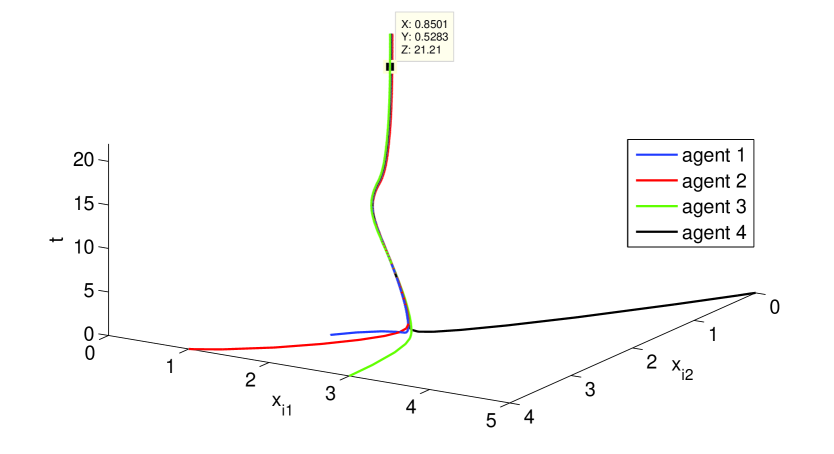
Figure 1: States’ trajectories for a ring network of single-integrator agents under the control law (15)

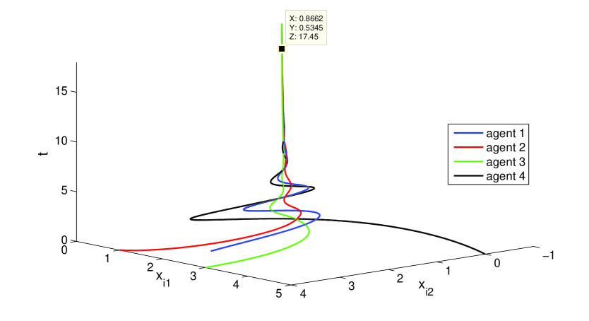
Figure 2: Simulation results of yi2015distributed : States’ trajectories for a ring network of single-integrator agents

References

- (1) Boyd, S., Vandenberghe, L.: Convex optimization. Cambridge university press (2004)
- (2) Cheng, L., Wang, H., Hou, Z.G., Tan, M.: Reaching a consensus in networks of high-order integral agents under switching directed topologies. International Journal of Systems Science 47(8), 1966–1981 (2016)
- (3) Fan, M.C., Chen, Z., Zhang, H.T.: Semi-global consensus of nonlinear second-order multi-agent systems with measurement output feedback. IEEE Transactions on Automatic Control 59(8), 2222–2227 (2014)
- (4) Feijer, D., Paganini, F.: Stability of primal–dual gradient dynamics and applications to network optimization. Automatica 46(12), 1974–1981 (2010)
- (5) Gharesifard, B., Cortés, J.: Distributed continuous-time convex optimization on weight-balanced digraphs. IEEE Transactions on Automatic Control 59(3), 781–786 (2014)
- (6) Horn, R.A., Johnson, C.R.: Matrix analysis. Cambridge university press (2012)
- (7) Khalil, H.: Nonlinear Systems. Prentice Hall (1996)
- (8) Kia, S.S., Cortés, J., Martínez, S.: Distributed convex optimization via continuous-time coordination algorithms with discrete-time communication. Automatica 55, 254–264 (2015)
- (9) Lin, P., Ren, W.: Constrained consensus in unbalanced networks with communication delays. IEEE Transactions on Automatic Control 59(3), 775–781 (2014)
- (10) Lu, J., Tang, C.Y.: Zero-gradient-sum algorithms for distributed convex optimization: The continuous-time case. IEEE Transactions on Automatic Control 57(9), 2348–2354 (2012)
- (11) Lygeros, J., Johansson, K.H., Simic, S.N., Zhang, J., Sastry, S.S.: Dynamical properties of hybrid automata. IEEE Transactions on automatic control 48(1), 2–17 (2003)
- (12) Nedic, A., Ozdaglar, A., Parrilo, P.A.: Constrained consensus and optimization in multi-agent networks. IEEE Transactions on Automatic Control 55(4), 922–938 (2010)
- (13) Niederländer, S.K., Cortés, J.: Distributed coordination for nonsmooth convex optimization via saddle-point dynamics. arXiv preprint arXiv:1606.09298 (2016)
- (14) Rahili, S., Ren, W.: Distributed continuous-time convex optimization with time-varying cost functions. IEEE Transactions on Automatic Control (2016)
- (15) Ren, W., Atkins, E.: Distributed multi-vehicle coordinated control via local information exchange. International Journal of Robust and Nonlinear Control 17(10-11), 1002–1033 (2007)
- (16) Rezaee, H., Abdollahi, F.: Average consensus over high-order multiagent systems. IEEE Transactions on Automatic Control 60(11), 3047–3052 (2015)
- (17) Ruszczynski, A.: Nonlinear optimization. Princeton University Press (2011)
- (18) Wang, J., Elia, N.: A control perspective for centralized and distributed convex optimization. In: 2011 50th IEEE Conference on Decision and Control and European Control Conference, pp. 3800–3805. IEEE (2011)
- (19) Xie, Y., Lin, Z.: Global optimal consensus for multi-agent systems with bounded controls. Systems & Control Letters 102, 104–111 (2017)
- (20) Yang, S., Liu, Q., Wang, J.: A multi-agent system with a proportional-integral protocol for distributed constrained optimization. IEEE Transactions on Automatic Control 62(7), 3461–3467 (2017)
- (21) Yi, P., Hong, Y., Liu, F.: Distributed gradient algorithm for constrained optimization with application to load sharing in power systems. Systems & Control Letters 83, 45–52 (2015)