Deep Bayesian Supervised Learning given Hypercuboidally-shaped, Discontinuous Data, using Compound Tensor-Variate $\&$ Scalar-Variate Gaussian Processes

Supplementary Material for ”Deep Bayesian Supervised Learning given Hypercuboidally-shaped, Discontinuous Data, using Compound Tensor-Variate and Scalar-Variate Gaussian Processes”

Abstract

We undertake Bayesian learning of the high-dimensional functional relationship between a system parameter vector and an observable, that is in general tensor-valued. The ultimate aim is Bayesian inverse prediction of the system parameters, at which test data is recorded. We attempt such learning given hypercuboidally-shaped data that displays strong discontinuities, rendering learning challenging. We model the sought high-dimensional function, with a tensor-variate Gaussian Process (GP), and use three independent ways for learning covariance matrices of the resulting likelihood, which is Tensor-Normal. We demonstrate that the discontinuous data demands that implemented covariance kernels be non-stationary–achieved by modelling each kernel hyperparameter, as a function of the sample function of the invoked tensor-variate GP. Each such function can be shown to be temporally-evolving, and treated as a realisation from a distinct scalar-variate GP, with covariance described adaptively by collating information from a historical set of samples of chosen sample-size. We prove that deep-learning using 2-”layers”, suffice, where the outer-layer comprises the tensor-variate GP, compounded with multiple scalar-variate GPs in the ”inner-layer”, and undertake inference with Metropolis-within-Gibbs. We apply our method to a cuboidally-shaped, discontinuous, real dataset, and subsequently perform forward prediction to generate data from our model, given our results–to perform model-checking.

journalname math.PR/0000000

, t2PhD student in Department of Mathematics, University of Leicester t1Lecturer in Statistics, Department of Mathematical Sciences, Loughborough University

1 Introduction

Statistical modelling allows for the learning of the relationship between two variables, where the said relationship is responsible for generating the data available on the variables. Thus, let $\boldsymbol{X}$ be a random variable that represents a behavioural or structural parameter of the system, and $\boldsymbol{Y}$ is another variable that bears influence on $\boldsymbol{X}$ s.t. $\boldsymbol{Y}=\boldsymbol{f}(\boldsymbol{X})$, where the functional relation $\boldsymbol{f}(\cdot)$ that we seek to learn, is itself a random structure, endowed with information about the error made in predicting the values of $\boldsymbol{Y}$ (or $\boldsymbol{X}$) at which the noise-included measurement of $\boldsymbol{X}$ (or $\boldsymbol{Y}$) has been realised. Such a function can be modelled as a realisation from an adequately chosen stochastic process. In general, either or both variables could be tensor-valued, such that, data comprising measurements of either variable, is then shaped as a hypercuboid. Typically, the structure/behaviour of a system is parametrised using a set of scalar-valued parameters, (say $d$ number of such parameters), which can, in principle be collated into a $d$-dimensional vector. Then $\boldsymbol{X}$ is typically, the system parameter vector. The other, observed variable $\boldsymbol{Y}$, can be tensor-valued in general. There are hypercuboidally-shaped data that show up in real-world applications, (Mardia and Goodall, 1993; Bijma et al., 2005; Werner et al., 2008; Theobald and Wuttke, 2008; Barton and Fuhrmann, 1993). For example, in computer vision, the image of one person might be a matrix of dimensions $a\times b$, i.e. image with resolution of $a$ pixels by $b$ pixels. Then, repetition across $n$ persons inflates the data to a cuboidally-shaped dataset. Examples of handling high-dimensional datasets within computer vision exist (Dryden et al., 2009; Fu, 2016; Pang et al., 2016; Wang, 2011; Qiang and Fei, 2011). In health care, the $p$ number of health parameters of $n$ patients, when charted across $k$ time-points, again generates a high-dimensional data, which gets further enhanced, if the experiment involves tracking for changes across $\ell$ groups of $n$ patients each, where each such group is identified by the level of intervention (Chari, Coe, Vucic, Lockwood and Lam, 2010; Clarke et al., 2008; Oberg et al., 2015; Chari, Thu, Wilson, Lockwood, Lonergan, Coe, Malloff, Gazdar, Lam, Garnis et al., 2010; Sarkar, 2015; Wang et al., 2015; Fan, 2017). Again, in ecological datasets, there could be $n$ spatial locations at each of which, $p$ traits of $k$ species could be tracked, giving rise to a high-dimensional data (Leitao et al., 2015; Warton, 2011; Dunstan et al., 2013).

It is a shortcoming of the traditional modelling strategies that we treated these groupings in the data as independent–or for that matter, even the variation in parameter values of any group across the $k$ time points, is ignored, and a mere snapshot of each group is traditionally considered, one at a time. In this work, we advance a method for the consideration of parameters across all relevant levels of measurement, within one integrated framework, to enable the learning of correlations across all such levels, thus permitting the prediction of the system parameter vector, with meaningful uncertainties, and avoid information loss associated with categorisation of data.

While discussing the generic methodology that helps address the problem of learning the inter-variable relationship $\boldsymbol{f}(\cdot)$, given general hypercuboid-shaped data, we focus on developing such learning when this data displays discontinuities. In such a learning exercise, the inter-variable functional relation $\boldsymbol{f}(\cdot)$, needs to be modelled using a high-dimensional stochastic process (a tensor-variate Gaussian Process, for example), the covariance function of which is non-stationary. The correlation between a pair of data slices, (defined by two such measured values of $\boldsymbol{Y}$, each realised at two distinct values of the system parameter $\boldsymbol{X}$), is sometimes parametrically modelled as a function of the distance between the values of the system parameter at which these slices are realised, i.e. “similarity” in values of $\boldsymbol{Y}$ can be modelled as a function of “similarity” in the corresponding $\boldsymbol{X}$ values. However, if there are discontinuities in the data, then such a mapping between “similarities” in $\boldsymbol{X}$ and $\boldsymbol{Y}$ no longer holds. Instead, discontinuities in data call for a model of the correlation that adapts to the discontinuities in the data. We present such correlation modelling in this paper, by modelling each scalar-valued hyperparameter of the correlation structure of the high-dimensional stochastic process, as a random function of the sample path of that process; this random function then, can itself be modelled as a realisation of a scalar-variate stochastic process–a scalar-variate Gaussian Process (GP) for example (Section 2).

Thus, the learning of $\boldsymbol{f}(\cdot)$ is double-layered, in which multiple scalar-variate GPs inform a high-dimensional (tensor-variate) GP. Importantly, we show below (Section 3.3) that no more than 2 such layers in the learning strategy suffice. Thus, the data on the observable $\boldsymbol{Y}$ can be shown to be sampled from a compound tensor-variate and multiple scalar-variate Gaussian Processes.

Acknowledgement of non-stationarity in correlation learning is not new (Paciorek and Schervish, 2004). In some approaches, a transformation of the space of the input variable is suggested, to accommodate non-stationarity (Sampson and Guttorp, 1992; Snoek et al., 2014; Schmidt and O’Hagan, 2003). When faced with learning the dynamically varying covariance structure of time-dependent data, others have resorted to learning such a covariance, using Generalised Wishart Process (Wilson and Ghahramani, 2011). In another approach, latent parameters that bear information on non-stationarity, have been modelled with GPs and learnt simultaneously with the sought function (Tolvanen et al., 2014), while others have used multiple GPs to capture the non-stationarity (Gramacy, 2005; Heinonen et al., 2016). However, what has not been presented, is a template for including non-stationarity in high-dimensional data, by nesting lower-dimensional Gaussian Processes with distinct covariances, within a tensor-variate GP (Section 2 and Section 3), using a Metropolis-within-Gibbs inference scheme (Section 4), to perform with-uncertainties learning of a high-dimensional function, given discontinuities that show up in the hypercuboidally-shaped datasets in general, and illustration of the method on a cuboidally-shaped, real-world dataset (Section 5, Section 6). This is what we introduce in this paper. Our model is capacitated to learn the temporally-evolving covariance of time-dependent data (Section 3.2), if such is the data at hand, but the focus of our interest is to follow the learning of the sought tensor-valued functional relation between a system parameter vector and a tensor-valued observable, with inverse Bayesian prediction of the system parameter values, at which test data on the observable is measured (Section 7, Section 6). Additionally, flexibility of our model design permits both inverse and forward predictions. So we also predict new data at chosen system parameter values given our model and results, and perform model checking, by comparing such generated data against the empirically observed data (Section 3 of Supplementary Materials).

2 Model

Let system parameter vector $\boldsymbol{S}\in{\boldsymbol{\cal X}}\subseteq{\mathbb{R}}^{d}$, be affected by observable $\boldsymbol{V}$, where $\boldsymbol{V}$ is ($k-1$-th ordered) tensor-valued in general, i.e. is $\boldsymbol{V}\in{\boldsymbol{\cal Y}}\subseteq{\mathbb{R}}^{m_{1}\times m_{2}\times\ldots\times m_{k-1}}$, $m_{i}\in{\mathbb{Z}},\forall\>i=1,\ldots,k-1$. That $\boldsymbol{V}$ bears influence on $\boldsymbol{S}$ suggests the relationship $\boldsymbol{V}=\boldsymbol{\xi}(\boldsymbol{S})$ where $\boldsymbol{\xi}:{\boldsymbol{\cal X}}\subseteq{\mathbb{R}}^{d}\longrightarrow{\boldsymbol{\cal Y}}\subseteq{\mathbb{R}}^{m_{1}\times m_{2}\times\ldots\times m_{k-1}}$.

Definition 2.1.

We define functional relationship $\boldsymbol{\xi}(\cdot)$, between $\boldsymbol{S}$ and $\boldsymbol{V}$, as a “tensor-valued function”, with $\displaystyle{\prod\limits_{i=1}^{k-1}m_{i}}$-number of component functions, where these components suffer inter-correlations. Thus, the learning of $\boldsymbol{\xi}(\cdot)$ is equivalent to learning the component functions, inclusive of learning the correlation amongst these component functions.

Inverse of $\boldsymbol{\xi}(\cdot)$, is defined as the tensor-valued function of same dimensionalities as $\boldsymbol{\xi}(\cdot)$, comprising inverses of each component function of $\boldsymbol{\xi}(\cdot)$, assuming inverse of each component function exists.

The inversion of the sought function $\boldsymbol{\xi}(\cdot)$–where $\boldsymbol{V}=\boldsymbol{\xi}(\boldsymbol{S})$–allows for the forward prediction of $\boldsymbol{v}^{(new)}$ given a measured value $\boldsymbol{s}^{(new)}$ of $\boldsymbol{S}$, as well as for the inverse prediction of the value of $\boldsymbol{S}$ at which a given measurement of $\boldsymbol{V}$ is recorded. It may be queried: why do we undertake the seemingly more difficult learning of the tensor-valued $\boldsymbol{\xi}(\cdot)$ (that outputs the tensor $\boldsymbol{V}$), than of the vector-valued $\boldsymbol{g}(\cdot)$ (that outputs the vector $\boldsymbol{S}$). We do this, because we want to retain the capacity of predicting both new data at a given value of the system parameter ($\boldsymbol{S}$), as well as predict the system parameter at which a new measurement of the observable $\boldsymbol{V}$ is realised.

Remark 2.1.

If we had set ourselves the task of learning $\boldsymbol{g}(\cdot)$, where $\boldsymbol{g}(\boldsymbol{V})=\boldsymbol{S}$, i.e. $\boldsymbol{g}(\cdot)$ is a “vector-valued” function, and therefore lower dimensional with fewer number of component functions than the tensor-valued $\boldsymbol{\xi}(\cdot)$–we could not have predicted value of $\boldsymbol{V}$ at a given $\boldsymbol{s}$. The $d$-dimensional vector-valued inverse function $\boldsymbol{g}^{-1}(\cdot)$ cannot yield a value of the $\displaystyle{\prod\limits_{i=1}^{k-1}m_{i}}$ number of components of the tensor $\boldsymbol{V}$ at this given $\boldsymbol{S}$, if $\displaystyle{\prod\limits_{i=1}^{k-1}m_{i}}>d$.

The learning of the function $\boldsymbol{\xi}(\cdot)$, uses the training data ${\bf D}:=\{(\boldsymbol{s}_{i},\boldsymbol{v}_{i})\}_{i=1}^{N}$. Conventional prediction of $\boldsymbol{S}=\boldsymbol{s}^{(test)}$, at which test data $\boldsymbol{v}^{(test)}$ on $\boldsymbol{V}$ is realised, suggests: $\boldsymbol{s}^{(test)}:=\boldsymbol{\xi}^{-1}(\boldsymbol{V})|_{\boldsymbol{v}^{(test)}}$.

• However, this there is no objective way to include the uncertainties learnt in the learning of the function $\boldsymbol{\xi}(\cdot)$, to propagate into the uncertainty of this prediction. This underpins an advantage of Bayesian prediction of one variable, given test data on the other, subsequent to learning of $\boldsymbol{\xi}(\cdot)$ using training data ${\bf D}$.

• Conventional fitting methods (such as fitting with splines, etc), also fumble when measurements of both/either of the r.v.s $\boldsymbol{S}$ and $\boldsymbol{V}$, are accompanied by measurement errors; in light of this, it becomes difficult to infer the function that fits the data the best. In fact, the uncertainty in the learning of the sought function is also then difficult to quantify.

• Secondly, there is no organic way of quantifying the smoothness of the sought $\boldsymbol{\xi}(\cdot)$, in th econventional approach. Ideally, we would prefer to learn this smoothness from the data itself. However, there is nothing intrinsic to the fitting-with-splines/wavelets method that can in principle, quantity the smoothness of the curve, given a training data.

• Lastly, when $\boldsymbol{V}$ is an r.v. that is no longer a scalar, but higher-dimensional (say tensor-valued in general), fitting with splines/wavelets starts to become useless, since in such cases of sought tensor-valued function $\boldsymbol{\xi}(\cdot)$ (in general), the component functions of $\boldsymbol{\xi}(\cdot)$ are correlated, but methods such as parametric fitting approaches, cannot capture such correlation, given the training data. As we have remarked above, such correlation amongst the components functions of $\boldsymbol{\xi}(\cdot)$ is the same correlation structure amongst the components of the tensor-valued $\boldsymbol{V}$–so in principle, the sought correlation can be learnt from the training data.

In light of this, we identify a relevant Stochastic Process that can give a general, non-restrictive description of the sought function $\boldsymbol{\xi}(\cdot)$–a Gaussian Process for example. The joint probability density of a set of realisations of a sampled $\boldsymbol{\xi}(\cdot)$, is then driven by the Process under consideration, where each such realisation of the function, equals a value of the output variable $\boldsymbol{V}$. Thus, the joint also represents the likelihood of the Process parameters given the relevant set of values of $\boldsymbol{V}$, i.e. the data. We impose judiciously chosen priors, to write the posterior probability density of the Process parameters given the data. Generating samples from this posterior then allows for the identification of the 95$\%$ HPD credible regions on these Process parameters, i.e. on the learnt function $\boldsymbol{\xi}(\cdot)$. It is possible to learn the smoothness of the function generated from this Process, via kernel-based parameterisation of the covariance structure of the GP under consideration. Thus, we focus on the pursuit of adequate covariance kernel parametrisation.

Proposition 2.1.

When possible, covariance matrices of the GP that is invoked to model the sought function $\boldsymbol{\xi}(\cdot)$, are kernel-parametrised using stationary-looking kernel functions, hyperparameters of which are modelled as dependent on the sample paths (or rather sample functions) of this GP. We show below (Lemma 3.1) that such a model can address the anticipated discontinuities in data.

As LHS of equation $\boldsymbol{V}=\boldsymbol{\xi}(\boldsymbol{S})$ is $k-1$-th ordered tensor-valued, $\boldsymbol{\xi}(\cdot)$ is tensor-variate function of equal dimensionalities. So we model $\boldsymbol{\xi}(\cdot)$ as a realisation from a tensor-variate GP.

Definition 2.2.

Modelling $\boldsymbol{\xi}(\cdot)$ as sampled from a tensor-variate GP, where the $k-1$-th ordered tensor-valued variable $\boldsymbol{V}=\boldsymbol{\xi}(\boldsymbol{S})$, we get that the joint probability of the set of values of sampled function $\boldsymbol{\xi}(\cdot)$, at each of the $n$ design points $\boldsymbol{s}_{1},\ldots\boldsymbol{s}_{n}$ (that reside within the training data ${\bf D}=\{(\boldsymbol{s}_{i},\boldsymbol{v}_{i})\}_{i=1}^{n}$), follows the $k$-variate Tensor Normal distribution (Kolda and Bader, 2009; Richter et al., 2008; McCullagh, 1987; Manceur and Dutilleul, 2013):

$$[\boldsymbol{\xi}(\boldsymbol{s}_{1}),\ldots,\boldsymbol{\xi}(\boldsymbol{s}_{n})]\sim{\cal TN}(\boldsymbol{M},\boldsymbol{\Sigma}_{1},\ldots,\boldsymbol{\Sigma}_{k}),$$

where mean of this density is a $k$-th ordered mean tensor $\boldsymbol{M}$ of dimensions $m_{1}\times\ldots\times m_{k}$, and $\boldsymbol{\Sigma}_{j}$ is the $m_{j}\times m_{j}$-dimensional, $j$-th covariance matrix; $j=1,\ldots,k$. In other words, likelihood of $\boldsymbol{M},\boldsymbol{\Sigma}_{1},\ldots,\boldsymbol{\Sigma}_{k}$ given ${\bf D}$ is the $k$-variate Tensor Normal density:

$${\cal L}(\boldsymbol{M},\boldsymbol{\Sigma}_{1},...,\boldsymbol{\Sigma}_{k}|{\bf D})\propto\exp(-\|({\bf D}_{\boldsymbol{V}}-\boldsymbol{M})\times_{1}\boldsymbol{A}_{1}^{-1}\times_{2}\boldsymbol{A}_{2}^{-1}...\times_{k}\boldsymbol{A}_{k}^{-1}\|^{2}/2),$$ (2.1)

where $n$ observed values of the $k-1$-th dimensional tensor-valued $\boldsymbol{V}$ are collated to form the $k$-th ordered tensor ${\bf D}_{\boldsymbol{V}}$. The notation $\times_{j}$ in Equation 2.1 presents the $j$-mode product of a matrix and a tensor (Oseledets, 2011). Here $\boldsymbol{A}_{j}$ is the unique square-root of the positive definite covariance matrix $\boldsymbol{\Sigma}_{j}$, i.e. $\boldsymbol{\Sigma}_{j}=\boldsymbol{A}_{j}\boldsymbol{A}^{T}_{j}$.

One example of a computational algorithm that can be invoked to realise such a square root of a matrix, is Cholesky decomposition.

We employ this likelihood in Equation 2.1 to write the joint posterior probability density of the mean tensor and covariance matrices, given the data. But prior to doing that, we identify those parameters–if any–that can be estimated in a pre-processing stage of the inference, in order to reduce the computational burden of inference. Also, it would be useful to find ways of (kernel-based) parametrisation of the sought covariance matrices, thereby reducing the number of parameters that we need to learn. To this effect, we undertake the estimation of the mean tensor is $\boldsymbol{M}\in R^{m_{1}\times m_{2}...\times m_{k}}$. It is empirically estimated as the sample mean $\overline{\boldsymbol{v}}$ of the sample $\{\boldsymbol{v}_{1},\ldots,\boldsymbol{v}_{n}\}$, s.t. $n$ repetitions of $\overline{\boldsymbol{v}}$ form the value $\boldsymbol{m}$ of $\boldsymbol{M}$. However, if necessary, the mean tensor itself can be regarded as a random variable and learnt from the data (Chakrabarty et al., 2015), The modelling of the covariance structure of this GP is discussed in the following subsection.

Ultimately, we want to predict the value of one variable, at which a new or test data on the other variable is observed.

Proposition 2.2.

To perform inverse prediction of value $\boldsymbol{s}^{(test)}$ of the input variable $\boldsymbol{S}$, at which test data $\boldsymbol{v}^{(test)}$ on $\boldsymbol{V}$ is realised, we will

1. sample from the posterior probability density of $\boldsymbol{s}^{(test)}$ given the test data $\boldsymbol{v}^{(test)}$, and (modal) values of the unknowns that parametrise the covariance matrices the high-dimensional GP invoked to model $\boldsymbol{\xi}(\cdot)$, subsequent to learning the marginals of each such unknown given the training data, using MCMC.

2. sample from the joint posterior probability density of $\boldsymbol{s}^{(test)}$ and all other unknowns parameters of this high-dimensional GP, given training, as well as test data, using MCMC.

Computational speed of the first approach, is higher, as marginal distributions of the GP parameters are learnt separately. When the training data is small, or if the training data is not representative of the test data at hand, the learning of $\boldsymbol{s}^{(test)}$ via the second method may affect the learning of the GP parameters.

2.1 3 ways of learning covariance matrices

Let the $ij$-th element of $p$-th covariance matrix $\boldsymbol{\Sigma}_{p}^{(m_{p}\times m_{p})}$ be $\sigma_{ij}^{(p)}$; $j,i=1,\ldots,m_{p}$, $p\in\{1,\ldots,k\}$.

Definition 2.3.

At a given $p$, $\sigma_{ij}^{(p)}$ bears information about covariance amongst the $i$-th and $j$-th slices of the $k$-th ordered data tensor ${\boldsymbol{D}}_{\boldsymbol{V}}=(\boldsymbol{v}_{1},\ldots,\boldsymbol{v}_{m_{p}})$, s.t. $m_{1}\times\ldots\times m_{p-1}\times m_{p+1}\times\ldots\times m_{k}$-dimensional $i$-th “slice” of data tensor $\boldsymbol{D}_{\boldsymbol{V}}$ is measured value $\boldsymbol{v}_{i}$ of $k-1$-th ordered tensor-valued $\boldsymbol{V}$, where the $i$-th slice is realised at the $i$-th design point $\boldsymbol{s}_{i}$.

The covariance between the $i$-th and $j$-th slices of data $\boldsymbol{D}_{\boldsymbol{V}}$ decreases as the slices get increasingly more disparate, i.e. with increasing $\parallel\boldsymbol{s}_{i}-\boldsymbol{s}_{j}\parallel$. In fact, we can model $\sigma_{ij}^{(p)}$ as a decreasing function $K_{p}(\cdot,\cdot)$ of this disparity $\parallel\boldsymbol{s}_{i}-\boldsymbol{s}_{j}\parallel$, where $K_{p}(\boldsymbol{s}_{i},\boldsymbol{s}_{j})$ is the covariance kernel function, computed at the $i$-th and $j$-th values of input variable $\boldsymbol{S}$. In such a model, the number of distinct unknown parameters involved in the learning of $\boldsymbol{\Sigma}_{p}$ reduces from $m_{p}(m_{p}+1)/2$, to the number of hyper-parameters that parametrise the kernel function $K_{p}(\cdot,\cdot)$.

However, kernel parametrisation is not always possible.
–Firstly, this parametrisation may cause information loss and this may not be acceptable
(Aston and Kirch, 2012).
–Again, we will necessarily avoid kernel parametrisation, when we cannot find input parameters, at which the corresponding slices in the data are realised.

In such situations,
–we can learn the elements of the covariance matrix directly using MCMC, though direct learning of all distinct elements of $\boldsymbol{\Sigma}_{p}$ is feasible, as long as total number of all unknowns learnt by MCMC $\lesssim 200$.
–we can use an empirical estimation for the covariance matrix $\boldsymbol{\Sigma}_{p}$. We collapse each of the $m_{p}$ number of $k-1$-th ordered tensor-shaped slices of the data, onto the $q$-th axis in the space ${\cal Y}$ of $\boldsymbol{V}$, where we can choose any one value of $q$ from $\{1,\ldots,k-1\}$. This will reduce each slice to a $m_{q}$-dimensional vector, so that $\sigma_{ij}^{(p)}$ is covariance computed using the $i$-th and $j$-th such $m_{q}$-dimensional vectors.

Indeed such an empirical estimate of any covariance matrix is easily generated, but it indulges in linearisation amongst the different dimensionalities of the observable $\boldsymbol{V}$, causing loss of information about the covariance structure amongst the components of these high-dimensional slices. This approach is inadequate when the sample size is small because the sample-based estimate will tend to be incorrect; indeed discontinuities and steep gradients in the data, especially in small-sample and high-dimensional data, will render such estimates of the covariance structure incorrect. Importantly, such an approach does not leave any scope for identifying the smoothness in the function $\boldsymbol{\xi}(\cdot)$ that represents the functional relationship between the input and output variables. Lastly, the uncertainties in the estimated covariance structure of the GP remain inadequately known.

Proposition 2.3.

We model the covariance matrices as
–kernel parametrised,
–or empirically-estimated,
–or learnt directly using MCMC.

An accompanying computational worry is the inversion of any of the covariance matrices; for a covariance matrix that is an $m_{p}\times m_{p}$-dimensional matrix, the computational order for matrix inversion is well known to be ${\cal O}(m^{3}_{p})$ (Knuth, 1997).

3 Kernel parametrisation

Proposition 3.1.

Kernel parametrisation of a covariance matrix, when undertaken, uses an Squared Exponential (SQE) covariance kernel

$$K(\boldsymbol{s}_{i},\boldsymbol{s}_{j}):=A\left[\exp\left(-(\boldsymbol{s}_{i}-\boldsymbol{s}_{j})^{T}\boldsymbol{Q}^{-1}(\boldsymbol{s}_{i}-\boldsymbol{s}_{j})\right)\right],\quad\forall i,j=1,\ldots,d,$$ (3.1)

where $\boldsymbol{Q}$ is a diagonal matrix, the diagonal elements of which are the length scale hyperparameters $\ell_{1},\ldots,\ell_{d}\in{\mathbb{R}}_{>0}$ that tell us how quickly correlation fades away in each of the $d$-directions in input space ${\cal X}$, s.t. the inverse matrix $\boldsymbol{Q}^{-1}$ is also diagonal, with the diagonal elements given as ${\displaystyle{\frac{1}{\ell_{1}},\ldots,\frac{1}{\ell_{d}}}}$, where $q_{c}:=1/\ell_{c}$ is the smoothness hyperparameter along the $c$-th direction in ${\cal X}$, $c=1,\ldots,d$. We learn these $d$ unknown parameters from the data.

Here $A$ is the global amplitude, that is subsumed as a scale factor, in one of the other covariance matrices, distinct elements of which are learnt directly using MCMC.

Remark 3.1.

We avoid using a model for the kernel in which amplitude depends on the locations at which covariance is computed, i.e. the model: $K(\boldsymbol{s}_{i},\boldsymbol{s}_{j}):=a_{ij}\left[\exp\left(-(\boldsymbol{s}_{i}-\boldsymbol{s}_{j})^{T}\boldsymbol{Q}^{-1}(\boldsymbol{s}_{i}-\boldsymbol{s}_{j})\right)\right]$, and use a model endowed with a global amplitude $A$. This helps avoid learning a very large number ($d(d+1)/2$) of amplitude parameters $a_{ij}$ directly from MCMC.

A loose interpretation of this amlitude modelling is that we have scaled all local amplitudes $a_{ij}$ to be $\leq 1$ using the global factor $A$ ($=\max\limits{ij}\{a_{ij}\}$), and these scaled local amplitudes are then subsumed into the argument of the exponential in the RHS of the last equation, s.t. the reciprocal of the correlation length scales, that are originally interpreted as the elements of the diagonal matrix $\boldsymbol{Q}^{-1}$, are now interpreted as the smoothing parameters modulated by such local amplitudes. This interpretation is loose, since the same smoothness parameter cannot accommodate all (scaled by a global factor) local amplitudes$\in(0,1]$, for all $\boldsymbol{s}_{i}-\boldsymbol{s}_{j}$.

3.1 Including non-stationarity, by modelling hyperparameters of covariance kernels as realisations of Stochastic Process

By definition of the kernel function we choose, (Equation 3.1), all functions $\boldsymbol{\xi}(\cdot)$ sampled from the tensor-variate GP, are endowed with the same length scale hyperparameters $\ell_{1},\ldots,\ell_{d}$, and global amplitude $A$. However, the data on the output variable $\boldsymbol{V}$ is not continuous, i.e. similarity between $\boldsymbol{s}_{i}$ and $\boldsymbol{s}_{j}$ does not imply similarity between $\boldsymbol{\xi}(\boldsymbol{s}_{i})$ and $\boldsymbol{\xi}(\boldsymbol{s}_{j})$, computed in a universal way $\forall\boldsymbol{s}_{i},\boldsymbol{s}_{j}\in{\cal X}$. Indeed, then a stationary definition of the correlation for all pairs of points in the function domain, is wrong. One way to generalise the model for the covariance kernel is to suggest that the hyperparameters vary as random functions of the sample path.

Theorem 3.1.

For ${\boldsymbol{V}}=\boldsymbol{\xi}(\boldsymbol{S})$, with $\boldsymbol{S}\in{\cal X}$ and $\boldsymbol{V}\in{\cal Y}$, if the map $\boldsymbol{\xi}:{\cal X}\longrightarrow{\cal Y}$ is a Lipschitz-continuous map over the bound set ${\cal X}\subseteq{\mathbb{R}}^{d}$, where absolute value of correlation between $\boldsymbol{\xi}(\boldsymbol{s}_{1})$ and $\boldsymbol{\xi}(\boldsymbol{s}_{2})$ is

$$|corr(\boldsymbol{\xi}(\boldsymbol{s}_{1}),\boldsymbol{\xi}(\boldsymbol{s}_{2}))|:=\displaystyle{K\left(\langle(\boldsymbol{s}_{1}-\boldsymbol{s}_{2}),\boldsymbol{q}\rangle^{2}\right)},\quad\forall\boldsymbol{s}_{1},\boldsymbol{s}_{2}\in{\cal X},$$

with

$$K(\boldsymbol{s}_{1},\boldsymbol{s}_{2}):=\displaystyle{\exp\left[-{\langle(\boldsymbol{s}_{1}-\boldsymbol{s}_{2}),\boldsymbol{q}\rangle^{2}}\right]},$$

then the vector $\boldsymbol{q}$ of correlation hyperparameters is finite, and each element of $\boldsymbol{q}$ is $\boldsymbol{\xi}$-dependent, i.e.

$$\boldsymbol{q}(\boldsymbol{\xi})=(q_{1}(\boldsymbol{\xi}),\ldots,q_{d}(\boldsymbol{\xi}))^{T}\in{\mathbb{R}}^{d}.$$

Proof.

For $\boldsymbol{S}\in{\cal X}$, where ${\cal X}$ is a bounded subset of ${\mathbb{R}}^{d}$, and $\boldsymbol{V}\in{\cal Y}$, the mapping $\boldsymbol{\xi}:{\cal X}\longrightarrow{\cal Y}$ is a defined to be Lipschitz-continuous map, i.e.

$$d_{\cal Y}(\boldsymbol{\xi}(\boldsymbol{s}_{1})-\boldsymbol{\xi}(\boldsymbol{s}_{2}))\leq L_{\boldsymbol{\xi}}d_{\cal X}(\boldsymbol{s}_{1},\boldsymbol{s}_{2}),\quad\forall\boldsymbol{s}_{1},\boldsymbol{s}_{2}\in{\cal X},$$ (3.2)

–for constant $L_{\boldsymbol{\xi}}\in{\mathbb{R}}$, s.t. the infinum over all such constants is the finite Lipschitz constant for $\boldsymbol{\xi}$;
–$({\cal X},d_{\cal X})$ and $({\cal Y},d_{\cal Y})$ are metric spaces.

Let metric $d_{\cal X}(\cdot,\cdot)$ be the $L_{2}$ norm:

$$d_{\cal X}(\boldsymbol{s}_{1},\boldsymbol{s}_{2}):=\parallel\boldsymbol{s}_{1}-\boldsymbol{s}_{2}\parallel,\quad\forall\boldsymbol{s}_{1},\boldsymbol{s}_{2}\in{\cal X},$$

and the metric $d_{\cal Y}(\boldsymbol{\xi}(\cdot),\boldsymbol{\xi}(\cdot))$ be defined as (square root of the logarithm of) the inverse of the correlation:

$$d_{\cal Y}(\boldsymbol{\xi}(\boldsymbol{s}_{1}),\boldsymbol{\xi}(\boldsymbol{s}_{2})):=\sqrt{-\log|corr(\boldsymbol{\xi}(\boldsymbol{s}_{1}),\boldsymbol{\xi}(\boldsymbol{s}_{2}))|},\quad\forall\boldsymbol{s}_{1},\boldsymbol{s}_{2}\in{\cal X},$$

–where correlation being a measure of affinity, $\log|1/corr(\cdot,\cdot)|$, transforms this affinity into a squared distance for this correlation model; so the transformation $\sqrt{\log|1/corr(\cdot,\cdot)|}$ to a metric is undertaken;
–and the given kernel-parametrised correlation is:

$$|corr(\boldsymbol{\xi}(\boldsymbol{s}_{1}),\boldsymbol{\xi}(\boldsymbol{s}_{2}))|:=\exp[-{\langle(\boldsymbol{s}_{1}-\boldsymbol{s}_{2}),\boldsymbol{q}\rangle}^{2}],\quad\forall\boldsymbol{s}_{1},\boldsymbol{s}_{2}\in{\cal X},\>\boldsymbol{q}\in{\mathbb{R}}^{d},$$

so that

$$d_{\cal Y}(\boldsymbol{\xi}(\boldsymbol{s}_{1}),\boldsymbol{\xi}(\boldsymbol{s}_{2}))={\langle(\boldsymbol{s}_{1}-\boldsymbol{s}_{2}),\boldsymbol{q}\rangle}.$$

Then for the map $\boldsymbol{\xi}$ to be Lipschitz-continuous, we require:

$${\sum\limits_{i=1}^{d}q_{i}^{2}(\boldsymbol{s}_{1}^{(i)}-\boldsymbol{s}_{2}^{(i)})^{2}}\leq\displaystyle{L_{\boldsymbol{\xi}}^{2}\sum\limits_{i=1}^{d}(\boldsymbol{s}_{1}^{(i)}-\boldsymbol{s}_{2}^{(i)})^{2}},$$ (3.3)

where the vector of correlation hyperparameters, $\boldsymbol{q}=(q_{1},\ldots,q_{d})^{T}$, is finite given finite $L_{\boldsymbol{\xi}}$.

By choosing to define

$$q_{max}:=\max(q_{1},\ldots,q_{d}),$$ (3.4)

and

$$(q_{i}^{{}^{\prime}})^{2}:=\displaystyle{\left(\frac{q_{i}}{q_{max}}\right)^{2}}\leq 1,\forall i=1,\ldots,d,$$

inequation 3.3 is valid, if we choose the $\xi$-dependent, Lipschitz constant $L_{\boldsymbol{\xi}}$ (that exists for this Lipschitz map) to be:

$$L_{\boldsymbol{\xi}}^{2}=q_{max}^{2},$$

i.e. the map $\boldsymbol{\xi}$ is Lipschitz-continuous, if $q_{max}$ is $\boldsymbol{\xi}$-dependent.
Then recalling definition, $q_{max}$ from Equation 3.4, it follows that in general, $q_{i}$ is $\boldsymbol{\xi}$-dependent, $\forall i=1,\ldots,d$. ∎

Given discontinuities in the data on $\boldsymbol{V}$, the function $\boldsymbol{\xi}(\cdot)$ is not expected to obey the Lipschitz criterion defined in inequation 3.2 globally. We anticipate sample function $\boldsymbol{\xi}(\cdot)$ to be locally or globally discontinuous.

Lemma 3.1.

Sample function $\boldsymbol{\xi}(\cdot)$ can be s.t.

1. $\exists\boldsymbol{s}_{2}\in{\cal X}$, s.t. $\nexists$ finite Lipschitz constant $L_{\boldsymbol{\xi}}^{(1,2)}>0$, for which $d_{\cal Y}(\boldsymbol{\xi}(\boldsymbol{s}_{1})-\boldsymbol{\xi}(\boldsymbol{s}_{2}))\leq L_{\boldsymbol{\xi}}^{(1,2)}d_{\cal X}(\boldsymbol{s}_{1},\boldsymbol{s}_{2})$. Here the bounded set ${\cal X}\subset{\mathbb{R}}^{d}$.

2. $\exists\boldsymbol{s}_{2},\boldsymbol{s}_{3}\in{\cal X}$, with $\parallel\boldsymbol{s}_{2}-\boldsymbol{s}_{1}\parallel\neq\parallel\boldsymbol{s}_{3}-\boldsymbol{s}_{1}\parallel$, s.t. $d_{\cal Y}(\boldsymbol{\xi}(\boldsymbol{s}_{1})-\boldsymbol{\xi}(\boldsymbol{s}_{2}))\leq L_{\boldsymbol{\xi}}^{(1,2)}d_{\cal X}(\boldsymbol{s}_{1},\boldsymbol{s}_{2})$, but $d_{\cal Y}(\boldsymbol{\xi}(\boldsymbol{s}_{1})-\boldsymbol{\xi}(\boldsymbol{s}_{3}))\leq L_{\boldsymbol{\xi}}^{(1,3)}d_{\cal X}(\boldsymbol{s}_{1},\boldsymbol{s}_{3})$; $L_{\boldsymbol{\xi}}^{(1,2)}\neq L_{\boldsymbol{\xi}}^{(1,3)}$. In such a case, the Lipschitz constant used for the sample function $\boldsymbol{\xi}(\cdot)$ is defined to be

   $$L_{\boldsymbol{\xi}}=\max\{L_{\boldsymbol{\xi}}^{(i,j)}\}_{i\neq j;\boldsymbol{s}_{i},\boldsymbol{s}_{j}\in{\cal X}}.$$

If each function in the set $\{\boldsymbol{\xi}_{1}(\cdot),\ldots,\boldsymbol{\xi}_{n}(\cdot)\}$ is
–either globally Lipschitz, or is as described in Case II,
–and Case I does not hold true, then
$\forall\boldsymbol{s}_{1},\boldsymbol{s}_{2}\in{\cal X},\>\>$ $\exists$ a finite $L_{max}>0$, where

$$L_{max}:=\max\limits_{\boldsymbol{\xi}}\{L_{\boldsymbol{\xi}_{1}},L_{\boldsymbol{\xi}_{2}},\ldots,L_{\boldsymbol{\xi}_{n}}\},$$

where $L_{\boldsymbol{\xi}_{i}}$ is the $i$-th Lipschitz constant defined for the $i$-th sample function $\boldsymbol{\xi}_{i}(\cdot)$, $i=1,\ldots,n$,
i.e. $\exists$ a finite Lipschitz constant for all $n$ sample functions.
$\Longrightarrow\exists$ a universal correlation hyperparameter vector $\boldsymbol{q}_{max}$ for all $n$ sample functions (=$L_{max}$, by Theorem 3.1).

Lemma 3.2.

Following on from Lemma 3.1, if for any $\boldsymbol{\xi}_{i}(\cdot)\in\{\boldsymbol{\xi}_{1}(\cdot),\ldots,\boldsymbol{\xi}_{n}(\cdot)\}$ Case I holds, $\Longrightarrow$ finite maxima of $\boldsymbol{\xi}_{i}(\cdot)\in\{\boldsymbol{\xi}_{1}(\cdot),\ldots,\boldsymbol{\xi}_{n}(\cdot)\}$ does not exist,
$\Longrightarrow\nexists$ a finite Lipschitz constant $L_{max}$ for all $n$ sample functions,
$\Longrightarrow\nexists$ a universal correlation hyperparameter vector $\boldsymbol{q}_{max}$, for all sample functions,
i.e. we need to model correlation hyperparameters to vary with the sample function.

Remark 3.2.

Above, $q_{1},\ldots,q_{d}$ are hyperparameters of the correlation kernel; they are interpreted as the reciprocals of the length-scales $\ell_{1},\ldots,\ell_{d}$, i.e. $\ell_{i}=1/q_{i},\forall i=1,\ldots,d$.

Remark 3.3.

If the map $\boldsymbol{\xi}:{\cal X}\longrightarrow{\cal Y}$ is Lipschitz-continuous, (i.e. if hyperparameters $q_{1},\ldots,q_{d}$ are $\boldsymbol{\xi}$-dependent, by Theorem 3.1), then by Kerkheim’s Theorem (Kerkheim, 1994), $\boldsymbol{\xi}$ is differentiable almost everywhere in ${\cal X}\subset{\mathbb{R}}^{d}$; this is a generalisation of Rademacher’s Theorem to metric differentials (see Theorem 1.17 in Hajlasz (2014)). However, in our case, the function $\boldsymbol{\xi}(\cdot)$ is not necessarily differentiable given discontinuities in the data on the observable $\boldsymbol{V}\in{\cal Y}$, and therefore, is not necessarily Lipschitz.

Thus, Theorem 3.1 and Lemma 3.1 negate usage of a universal correlation length scale independent of sampled function $\boldsymbol{\xi}(\cdot)$, in anticipation of discontinuities in the sample function.

Proposition 3.2.

For ${\boldsymbol{V}}=\boldsymbol{\xi}(\boldsymbol{S})$, with $\boldsymbol{S}\in{\cal X}\subseteq{\mathbb{R}}^{d}$ and $\boldsymbol{V}\in{\cal Y}\subseteq{\mathbb{R}}^{(m_{1}\times\ldots\times m_{k})}$,

$$|corr(\boldsymbol{\xi}(\boldsymbol{s}_{1}),\boldsymbol{\xi}(\boldsymbol{s}_{2}))|:=\displaystyle{\exp\left[-{\langle(\boldsymbol{s}_{1}-\boldsymbol{s}_{2}),\boldsymbol{q}({\boldsymbol{\xi}})\rangle^{2}}\right]},\quad\forall\boldsymbol{s}_{1},\boldsymbol{s}_{2}\in{\cal X},$$

where $\boldsymbol{\xi}(\cdot)$ is a sample function of a tensor-variate GP. Thus, in this updated model, $c$-th component $q_{c}=1/\ell_{c}$ of correlation hyperparameter $\boldsymbol{q}({\boldsymbol{\xi}})$ is modelled as randomly varying with the sample function, $\boldsymbol{\xi}(\cdot)$, of the tensor-variate GP, $\forall c=1,\ldots,d$.
In the Metropolis-within-Gibbs-based inference that we undertake, one sample function of the tensor-variate GP generated, in every iteration, $\Longrightarrow q_{c}$ that we model above

as randomly varying with the sample path of the tensor-variate GP,

$$\equiv{\mbox{is randomly varying with the iteration number variable}}\quad T\in\{0,1,\ldots,t_{max}\}\subset{\mathbb{Z}}_{\geq 0},$$

$$\Longrightarrow{\mbox{We model}}\quad\ell_{c}=g_{c}(t),\quad c=1,\ldots,d,$$

where this scalar-valued random function $g_{c}:\{0,1,\ldots,t_{max}\}\subset{\mathbb{Z}}_{>0}\longrightarrow{\mathbb{R}}_{\geq 0}$, is modelled as a realisation from a scalar-variate GP.

Scalar-variate GP that $g_{c}(\cdot)$ is sampled from, is independent of the GP that $g_{c^{\prime}}(\cdot)$ is sampled from; $c\neq c^{\prime};c,c^{\prime}=1,\ldots,d$. In addition, parameters that define the correlation function of the generative scalar-variate GP can vary, namely the amplitude $A$ and scale $\delta$ of one such GP might be different from another. Thus, scalar-valued functions sampled from GPs with varying correlation parameters $A$ and $\delta$–even for the same $c$ value–should be marked by these descriptor variables $A>0$ and $\delta>0$.

Proposition 3.3.

We update the relationship between iteration number $T$ and correlation length scale hyperparameter $\ell_{c}$ in the $c$-th direction in input space to be:

$$\ell_{c}=g_{c,\boldsymbol{x}}(t),\quad{\mbox{where vector of descriptor variables is}}\quad\boldsymbol{X}:=(A,\delta)^{T},\quad{with}$$

–$A_{c}$ the amplitude variable of the SQE-looking covariance function of the scalar-variate GP that $g_{c,\boldsymbol{x}}(\cdot)$ is a realisation of. $A_{c}$ takes the value $a_{c}\geq 0$;
–$\delta_{c}$ the length scale variable of the SQE-looking covariance function of the scalar-variate GP that $g_{c,\boldsymbol{x}}(\cdot)$ is a realisation of; $\delta_{c}\in{\mathbb{R}}_{>0}$.
Then the scalar-variate GPs that $g_{c,\boldsymbol{x}}(\cdot)$ and $g_{c,\boldsymbol{x}^{/}}(\cdot)$ are sampled from, have distinct correlation functions if $\boldsymbol{x}\neq\boldsymbol{x}^{/}$. Here $c=1,\ldots,d$.

Proposition 3.4.

Current value of correlation length scale hyperparameter $\ell_{c}$, acknowledges information on only the past $t_{0}$ number of iterations as in:

$$\ell_{c} = g_{c,\boldsymbol{x}}(t-t^{{}^{\prime}}),\quad{\mbox{if}}\>\>t\geq t_{0},\>\>c=1,\ldots,d;\>t^{{}^{\prime}}=1,\ldots,t_{0},$$

$$\ell_{c} = \ell_{c}^{(const)},\quad{\mbox{if}}\>\>t=0,1,\ldots,t_{0}-1,\>\>\quad c=1,\ldots,d,$$ (3.5)

where $\ell_{c}^{(const)}$ is an unknown constant that we learn from the data, during the first $t_{0}$ iterations.

As $g_{c,\boldsymbol{x}}(t)$ is a realisation from a scalar-variate GP, the joint probability distribution of $t_{0}$ number of values of the function $g_{c,\boldsymbol{x}}(t)$–at a given $\boldsymbol{x}=(a,\delta)^{T}$–is Multivariate Normal, with $t_{0}$-dimensional mean vector $\boldsymbol{M}_{c,\boldsymbol{x}}$ and $t_{0}\times t_{0}$-dimensional covariance matrix $\boldsymbol{\Psi}_{c,\boldsymbol{x}}$, i.e.

$$[g_{c,\boldsymbol{x}}(t-1),\ldots,g_{c,\boldsymbol{x}}(t-2),g_{c,\boldsymbol{x}}(t-t_{0})]\sim{\cal MN}(\boldsymbol{M}_{c,\boldsymbol{x}},\boldsymbol{\Psi}_{c,\boldsymbol{x}}).$$ (3.6)

Definition 3.1.

Here $t_{0}$ is the number of iterations that we look back at, to collect the dynamically-varying “look back-data” ${\bf D}_{c,t}^{(orig)}:=\{\ell_{c,t-t_{0}},\ldots,\ell_{c,t-1}\}$ that is employed to learn parameters of the scalar-variate GP that $g_{c,\boldsymbol{x}}(\cdot)$ is modelled with.

1. The mean vector $\boldsymbol{M}_{c,\boldsymbol{x}}$ is empirically estimated as the mean of the dynamically varying look back-data, s.t. at the $t$-th iteration it is estimated as a $t_{0}$-dimensional vector with each component ${\hat{m}}_{c,\boldsymbol{x}}^{(t)}:=[\ell_{c,t-t_{0}}+\ldots+\ell_{c,t-1}]/t_{0}$.

2. $t_{0}\times t_{0}$-dimensional covariance matrix is dependent on the iteration-number and this is now acknowledged in the notation to state: $\boldsymbol{\Psi}_{c,\boldsymbol{x}}(t)=\left[a_{c}\exp\left(-\frac{(t_{i}-t_{j})^{2}}{\delta_{c}^{2}}\right)\right],\>i,j=t-1,\ldots,t-t_{0}$.

In the $t$-th iteration, upon the empirical estimation of the mean as given above, it is subtracted from the “look back-data” ${\bf D}_{c,t}^{(orig)}$ so that the subsequent mean-subtracted look back-data is ${\bf D}_{c,t}:=\{\ell_{c,t-t_{0}}-{\hat{m}}_{c,\boldsymbol{x}}^{(t)},\ldots,\ell_{c,t-1}-{\hat{m}}_{c,\boldsymbol{x}}^{(t)}\}$. It is indeed this mean-subtracted sample that we use.

Definition 3.2.

In light of this declared usage of the mean-subtracted “look back-data” ${\bf D}_{c,t}$, we update the likelihood over what is declared in Equation 3.6, to

$$[g_{c,\boldsymbol{x}}(t-1),\ldots,g_{c,\boldsymbol{x}}(t-2),g_{c,\boldsymbol{x}}(t-t_{0})]\sim{\cal MN}(\b{0},\boldsymbol{\Psi}_{c,\boldsymbol{x}}(t)),\quad\forall c=1,\ldots,d.$$ (3.7)

3.2 Temporally-evolving covariance matrix

Theorem 3.2.

The dynamically varying covariance matrix of the Multivariate Normal likelihood in Equation 3.7, at iteration number $t\geq t_{0}$, is

$$\boldsymbol{\Psi}_{c,\boldsymbol{x}}(t)\sim\displaystyle{{\cal GWP}(d,\boldsymbol{G}_{c},k(\cdot,\cdot))},\quad where:$$

the number of iterations we look back to is $t_{0}$;
$k(\cdot,\cdot)$ is the covariance kernel parametrising the covariance function of the scalar-variate GP that generates the scalar-valued function $g_{c,\boldsymbol{x}}(\cdot)$, at the vector $\boldsymbol{x}=(a_{c},\delta_{c})^{T}$ of descriptor variables, s.t. $k(t_{i},t_{j})=\exp\left(-\frac{(t_{i}-t_{j})^{2}}{\delta_{c}^{2}}\right),\>\forall t_{i},t_{j}=t-1,\ldots,t-t_{0}$;
$\boldsymbol{G}_{c}$ is a positive definite square scale matrix $\boldsymbol{G}_{c}$ of dimensionality $t_{0}$, containing the amplitudes of this covariance function;
$c=1,\ldots,d$, with the space ${\cal X}$ of input variable $\boldsymbol{S}$ $d$-dimensional.

Proof.

The covariance kernel $k(\cdot,\cdot)$ that parametrises the covariance function of the scalar-variate GP that generates $g_{c,\boldsymbol{x}}(t)$, is s.t. $k(t_{i},t_{i})$=1 $\forall i=1,\ldots,t_{0}$.

In a general model, at each iteration, a new value of the vector $\boldsymbol{x}_{c}$ of descriptor variables in the $c$-th direction in the space ${\cal X}$ of the input variable $\boldsymbol{S}$, is generated, s.t. in the $t-t_{i}$-th iteration, it is $\boldsymbol{x}_{c,i}=(a_{c,i},\delta_{c,i})^{T}$; $t-t_{i}=t-1,\ldots,t-t_{0}$

$$\Longrightarrow{\mbox{at}}\quad T=t,\quad\{g_{c,\boldsymbol{x}_{1}}(t),\ldots,g_{c,\boldsymbol{x}_{t_{0}}}(t)\}\quad{\mbox{is a sample of the random variable}}\quad g_{c,\boldsymbol{x}}(t).$$

Now, $corr(g_{c,\boldsymbol{x}}(t-t_{i}),g_{c,\boldsymbol{x}}(t-t_{j}))=k(t_{i},t_{j})\delta({c,c^{/}})\delta({\boldsymbol{x},\boldsymbol{x}^{/}})$, where $\delta({\cdot,\cdot})$ is the Delta function.
$\Longrightarrow$ sample estimate of $Cov(g_{c,\boldsymbol{x}}(t-t_{i}),g_{c,\boldsymbol{x}}(t-t_{j}))$ is

$$Cov(g_{c,\boldsymbol{x}}(t-t_{i}),g_{c,\boldsymbol{x}}(t-t_{j}))=\displaystyle{\sum\limits_{k=1}^{t_{0}}a_{c,i}a_{c,j}g_{c,\boldsymbol{x}_{k}}(t-t_{i})g_{c,\boldsymbol{x}_{k}}(t-t_{j})},\quad\forall t-t_{i},t-t_{j}=t-1,\ldots,t-t_{0},$$

is the $ij$-th element of matrix $\boldsymbol{\Psi}_{c,\boldsymbol{x}}(t)$.
This definition of the covariance holds since mean of the r.v. $g_{c,\boldsymbol{x}}(t)$ is 0, as we have sampled the function from a zero-mean scalar-variate GP.

$${\mbox{Let}}\quad\boldsymbol{g}_{c,\boldsymbol{x}_{k}}(t):=(g_{c,\boldsymbol{x}_{k}}(t-t_{1}),\ldots,g_{c,\boldsymbol{x}_{t_{k}}}(t-t_{0}))^{T},\quad k=1,\ldots,t_{0}.$$

Let $\boldsymbol{G}_{c}$ be a $t_{0}\times t_{0}$-dimensional diagonal matrix, the $i$-th diagonal element of which is $a_{c,i}^{2}$. Then factorising the scale matrix $\boldsymbol{G}_{c}=\boldsymbol{L}_{G_{c}}\boldsymbol{L}_{G_{c}}^{T}$, $\boldsymbol{L}_{G_{c}}$ is diagonal with the $i$-th diagonal element $a_{c,i}$; $i=1,\ldots,t_{0}$. This is defined for every $c\in\{1,\ldots,d\}$.

Then at iteration number $T=t$, we define the current covariance matrix

$$\boldsymbol{\Psi}_{c,\boldsymbol{x}}(t):=\displaystyle{\sum\limits_{k=1}^{t_{0}}\boldsymbol{L}_{G_{c}}\left(\boldsymbol{g}_{c,\boldsymbol{x}_{k}}(t)\right)^{T}\boldsymbol{g}_{c,\boldsymbol{x}_{k}}^{T}(t)\boldsymbol{L}_{G_{c}}^{T}}.$$

Then $\boldsymbol{\Psi}_{c,\boldsymbol{x}}(t)$ is distributed according to the Wishart distribution w.p, $\boldsymbol{G}_{c}$ and $d$ (Eaton, 1990), i.e. the dynamically-varying covariance matrix is:

$$\boldsymbol{\Psi}_{c,\boldsymbol{x}}(t)\sim{\cal{GWP}}(d,\boldsymbol{G}_{c},k(\cdot,\cdot)).$$

∎

Remark 3.4.

If interest lies in learning the covariance matrix at any time point, we could proceed to inference here from, in attempt of the learning of the unknown parameters of this ${\cal{GWP}}$ process given the lookback-data ${\bf D}_{c,t}$.

Our learning scheme then would then involve compounding a Tensor-Variate GP and a ${\cal{GWP}}$.

The above would be a delineated route to recover the temporal variation in the correlation structure of time series data (as studied, for example by Wilson and Ghahramani (2011)).

Remark 3.5.

In our study, the focus is on high-dimensional data that display discontinuities, and on learning the relationship $\boldsymbol{\xi}(\cdot)$ between the observable $\boldsymbol{V}$ that generates such data, and the system parameter $\boldsymbol{S}$–with the ulterior aim being parameter value prediction. So learning the time-varying covariance matrix $\Psi(t)$ is not the focus of our method development.

We want to learn $\boldsymbol{\xi}(\cdot)$ given training data ${\bf D}$. The underlying motivation is to sample a new $g_{c,\boldsymbol{x}}(\cdot)$ from a scalar-variate GP, at new values of $a_{1},\ldots,a_{d},\delta_{1},\ldots,\delta_{d}$, to subsequently sample a new tensor-valued function $\boldsymbol{\xi}(\cdot)$, from the tensor-normal GP, at a new value of its $d$-dimensional correlation length scale hyperparameter vector $\boldsymbol{\ell}$.

3.3 2-layers suffice

One immediate concern that can be raised is the reason for limiting the layering of our learning scheme to only 2. It may be argued that just as we ascribe stochasticity to the length scales $\ell_{1},\ldots,\ell_{d}$ that parametrise the correlation structure of the tensor-variate GP that models $\boldsymbol{\xi}(\cdot)$, we need to do the same to the descriptor variables $a,\>\delta$ that parametrise the correlation structure of the scalar-variate GP that model $g_{c,\boldsymbol{x}}(t)$. Following this argument, we would need to hold $a,\>\delta$–or at least model the scale $\delta$–to be dependent on the sample path of the scalar-variate GP, i.e. set $\delta$ to be dependent on $g_{c,\boldsymbol{x}}(\cdot)$.

However, we show below that a global choice of $\delta$ is possible irrespective of the sampled function $g_{c,\boldsymbol{x}}(\cdot)$, given that $g_{c,\boldsymbol{x}}:\{t-1,\ldots,t-t_{0}\}\subset{\mathbb{Z}}_{\geq 0}\longrightarrow{\mathbb{R}}_{\geq 0}$ is always continuous (a standard result). In contrast, the function $\boldsymbol{\xi}(\cdot)$ not being necessarily Lipschitz (see Remark 3.3), implies that the correlation kernel hyperparameters $q_{c}$, are $\boldsymbol{\xi}$-dependent, $\forall c=1,\ldots,d$.

Theorem 3.3.

Given $\ell_{c}=g_{c,\boldsymbol{x}}(t)$, with $T\in{\cal N}\subset{\mathbb{Z}}_{\geq 0}$ and $\ell_{c}\in{\mathbb{R}}$, the map $g_{c,\boldsymbol{x}}:{\mathbb{Z}}_{\geq 0}\longrightarrow{\mathbb{R}}_{\geq 0}$ is a Lipschitz-continuous map, $\forall c=1,\ldots,d$. Here ${\cal N}:=\{t-t_{1},\ldots,t-t_{0}\}$

The proof of this standard theorem is provided in Section 4 of the supplementary Materials.

Theorem 3.4.

For any sampled function $g_{c,\boldsymbol{x}}:{\cal N}\longrightarrow{\mathbb{R}}_{\geq 0}$ realised from a scalar-variate GP that has a covariance function that is kernel-parametrised with an SQE kernel function, parametrised by amplitude and scale hyperparameters, the Lipschitz constant that defines the Lipschitz-continuity of $g_{c,\boldsymbol{x}}(\cdot)$, is $g_{c,\boldsymbol{x}}$-dependent, and is given by the reciprocal of the scale hyperparameter, s.t. the set of $t_{0}$ values of scale hyperparameters, for each of the $t_{0}$ samples of $g_{c,\boldsymbol{x}}(\cdot)$ taken from the scalar-variate GP, admits a finite minima.

Proof.

For $\ell_{c}=g_{c,\boldsymbol{x}}(T)$, $g_{c,\boldsymbol{x}}:{\cal N}\subset{\mathbb{Z}}_{\geq 0}\longrightarrow{\cal G}\subset{\mathbb{R}}_{\geq 0}$ is a Lipschitz-continuous map, (Theorem 12.1), with $T\in{\cal N}$ and $\ell_{c}\in{\cal G}$. (${\cal N}$ is defined in Theorem 12.1). Distance between any $t-t_{1},t-t_{2}\in{\cal N}$ is given by metric

$$d_{\cal N}(t-t_{1},t-t_{2}):=|t_{1}-t_{2}|.$$

Distance between $g_{c,\boldsymbol{x}}(t-t_{1})$ and $g_{c,\boldsymbol{x}}(t-t_{2})$ is given by metric

$$d_{\cal G}(g_{c,\boldsymbol{x}}(t-t_{1}),g_{c,\boldsymbol{x}}(t-t_{2})):=\sqrt{-\log|corr(g_{c,\boldsymbol{x}}(t-t_{1}),g_{c,\boldsymbol{x}}(t-t_{2}))|},$$

s.t. $d_{\cal G}(g_{c,\boldsymbol{x}}(t-t_{1}),g_{c,\boldsymbol{x}}(t-t_{2}))\geq 0$, and is finite (since $t-t_{1},t-t_{2}$ live in a bound set, and $g_{c\boldsymbol{x}}(\cdot)$ is continuous). The parametrised model of the correlation is

$$|corr(g_{c,\boldsymbol{x}}(t-t_{1}),g_{c,\boldsymbol{x}}(t-t_{2}))|:=\displaystyle{K\left(\frac{(t_{1}-t_{2})^{2}}{\delta_{g}^{2}}\right)}\equiv\displaystyle{\exp\left[-\frac{(t_{1}-t_{2})^{2}}{\delta_{g}^{2}}\right]},$$

s.t. $|corr(g_{c,\boldsymbol{x}}(t-t_{1}),g_{c,\boldsymbol{x}}(t-t_{2}))|\in(0,1]$, where $\delta_{g}>0$ is the scale hyperparameter.

Now, Lipschitz-continuity of $g_{c,\boldsymbol{x}}(\cdot)$ implies

$$d_{\cal G}(g_{c,\boldsymbol{x}}(t-t_{1}),g_{c,\boldsymbol{x}}(t-t_{2}))\leq L_{g}d_{\cal N}(t-t_{1},t-t_{2}),$$ (3.8)

where the Lipschitz constant $L_{g}$ is $g_{c,\boldsymbol{x}}$-dependent (Theorem 3.1). As $d_{\cal N}(t-t_{1},t-t_{2})\equiv|t_{1}-t_{2}|\leq t_{0}$, where $t_{0}$ is a known finite integer, and as $d_{\cal G}(\cdot,\cdot)$ is defined as $|t_{1}-t_{2}|/\delta_{g},\>\delta_{g}>0$ (using definition of $d_{\cal G}(\cdot,\cdot)$), $L_{g}$ exists for $t_{1},t_{2}$, and is finite. We get

$$L_{g}=\displaystyle{\frac{1}{\delta_{g}}}.$$ (3.9)

As $t-t_{1},t-t_{2}$ is any point in ${\cal N}$, $L_{g}$ exists for all points in ${\cal N}$.

Let set $\boldsymbol{L}:=\{L_{g_{1}},\ldots,L_{g_{t_{0}}}\}$, where $L_{g_{i}}$ defines the Lipschitz-continuity condition (inequation 3.8) for the $i$-th sample function $g_{i}(\cdot)$ from a scalar-variate GP.

$$\exists L_{max}:={\displaystyle{\max_{g}}}[\boldsymbol{L}]={\displaystyle{\max_{g}}}\{L_{g_{1}},\ldots,L_{g_{t_{0}}}\},\quad{\mbox{where}}\quad L_{max}>0\quad{\mbox{and is finite.}}$$

Thus, $L_{max}$ is a Lipschitz constant that defines the Lipschitz continuity for any sampled function in $\{g_{c,\boldsymbol{x}}(t-t_{1}),\ldots,g_{c,\boldsymbol{x}}(t-t_{0})\}$, at any iteraion number $t$ in a chain of finite and known number of iterations.
Then by Equation 3.9, $\exists\delta>0$, s.t.

$$\delta:={\displaystyle{\max_{g}}\left\{\frac{1}{\delta_{g_{1}}},\ldots,\frac{1}{\delta_{g_{t_{0}}}}\right\}}={\displaystyle{\min_{g}}\{{\delta_{g_{1}}},\ldots,{\delta_{g_{t_{0}}}}\}};\quad{\mbox{where}}\>\delta_{g_{i}}>0\forall i=1,\ldots,t_{0}.$$

Here $L_{g_{i}}=\displaystyle{\frac{1}{\delta_{g_{i}}}};\>i=1,\ldots,t_{0}$. ∎

Theorem 3.5.

Given $\ell_{c}=g_{c,\boldsymbol{x}}(t)$, where $g_{c,\boldsymbol{x}}:{\cal N}\longrightarrow{\cal G}$ is a Lipschitz-continuous function, sampled from a scalar-variate GP, the covariance function of which, computed at any 2 points $t-t_{1},t-t_{2}$ in the input space ${\cal N}$, is kernel parametrised as

$$Cov(t_{1},t_{2})=\displaystyle{a_{c}K\left(\frac{(t_{1}-t_{2})^{2}}{\delta_{c}^{2}}\right)}\equiv\displaystyle{a_{c}\left(\exp\left[-\frac{(t_{1}-t_{2})^{2}}{\delta_{c}^{2}}\right]\right)},$$

where ($a_{c}$, the amplitude hyperparameter and) the scale hyperparameter of this kernel is $\delta_{c}$ that is independent of the sample function $g_{c,\boldsymbol{x}}(\cdot)$; $c\in\{1,\ldots,d\}$.

Proof.

By Theorem 3.4, $\delta_{c}:={\displaystyle{\min_{g_{c}}}\{{\delta_{g_{c,1}}},\ldots,{\delta_{g_{c,n}}}\}}$ exists for any $c\in\{1,\ldots,d\}$. Then the scalar-variate GP that models the sample function $g_{c,\boldsymbol{x}}(\cdot)$ has a covariance kernel that is marked by the finite scale hyperparameter $\delta_{c}$, independemt of the sample function. ∎

Remark 3.6.

That a stationary scale hyperparameter $\delta$ that is independent of the sample path can define the covariance kernel of the scalar-variate GP that $g_{c,\boldsymbol{x}}(\cdot)$ is sampled from, owes to the fact that any such sample function $g_{c,\boldsymbol{x}}(\cdot)$ is continuous given the nature of the map (from a subset of integers to reals). However, when the sample function from a GP is not continuous, (such as $\boldsymbol{\xi}(\cdot)$ that is modelled with the tensor-variate GP discussed above), a set of values of the sample function-dependent scale hyperparameter(s) of the covariance kernel of the corresponding GP, will not admit a minima, and therefore, in such a case, a global scale hyperparameter cannot be ascribed to the covariance kernel of the generating GP. This is why we need to retain the correlation length scale hyperparameter $\ell_{c}$ to be dependent on the tensor-valued sample function $\boldsymbol{\xi}(\cdot)$, but the scale hyperparameter $\delta_{c}$ is no longer dependent on the scalar-valued sample function $g_{c,\boldsymbol{x}}(\cdot)$. In other words, we do not require to add any further layers to our learning strategy, than the two layers discussed.

3.4 Learning using a Compound Tensor-Variate $\&$ Scalar-Variate GPs

We find inference defined by a sequential sampling from the scalar-variate GPs (for each of the $d$ directions of input space), followed by that from tensor-variate GP, directly relevant to our interests. Thus our learning involves a Compound tensor-variate and multiple scalar-variate GPs. To abbreviate, we will refer below to such a Compound Stochastic Process, as a “$nested-GP$” model.

Remark 3.7.

As $\delta_{c},a_{c}$ are not stochastic, hereon, we absorb the dependence of the function $g(\cdot)$ on the direction index, via the descriptor parameters, and refer to this function as $g_{\boldsymbol{x}_{c}}(t)$; $c=1,\ldots,d$.

Definition 3.3.

$Nested-GP$ model:
for $\boldsymbol{V}=\boldsymbol{\xi}(\boldsymbol{S})$,

$$\boldsymbol{\xi}(\cdot)\sim{\mbox{tensor-variate GP}},$$

s.t. joint probability of $n$ observations of $k-1$-th ordered tensor-valued variable $\boldsymbol{V}$ (that comprise training data ${\bf D}$), is $k$-th ordered Tensor Normal, with $k$ covariance matrices–which are empirically estimated, or learnt directly using MCMC, or kernel parametrised, s.t. length scale parameter $\ell_{1},\ldots,\ell_{d}$ of this covariance kernel, is each modelled as a dynamically varying function $\ell_{c}=g_{\boldsymbol{x}_{c}}(t)$, where

$$g_{\boldsymbol{x}_{c}}(t)\sim\>c-{\mbox{th scalar-variate GP}},$$

$\Longrightarrow$joint probability of the last $t_{0}$ observations of $\ell_{c}$ (that comprise “lookback data” ${\bf D}_{c,t}$), is Multivariate Normal, the covariance function of which is parametrised by a kernel indexed by the $c$-th, stationary descriptor parameter vector $\boldsymbol{x}_{c}=(a_{c},\delta_{c})^{T}$, where $a_{c}$ is the amplitude and $\delta_{c}$ the scale-length hyperparameter of the SQE-looking covariance kernel; $c=1,\ldots,d$.

Definition 3.4.

$Nonnested-GP$ model:
for $\boldsymbol{V}=\boldsymbol{\xi}(\boldsymbol{S})$,

$$\boldsymbol{\xi}(\cdot)\sim{\mbox{tensor-variate GP}},$$

s.t. joint probability of observations of $\boldsymbol{V}$ is $k$-th ordered Tensor Normal, with $k$ covariance matrices–which are empirically estimated, or learnt directly using MCMC, or kernel parametrised, s.t. length scale parameter $\ell_{1},\ldots,\ell_{d}$ of this covariance kernel, is each treated as a stationary unknown. All learning is undertaken using training data ${\bf D}$.

4 Inference

We undertake inference with Metropolis-within-Gibbs. Below $\theta^{(t\star)}$ indicates proposed value of parameter $\theta$ in the $t$-th iteration, while $\theta^{(t)}$ refers to the value current in the $t$-th iteration.

• $Nested-GP$:

  1. In $t>t_{0}$-th iteration, propose amplitude and scale-length of $c$-th scalar-variate GP as:

     $$a_{c}^{(t\star)}\sim{\cal TN}(a_{c}^{(t-1)},0,v_{a}^{(c)}),\quad\forall c=1,\ldots,d,$$

     $$\delta_{c}^{(t\star)}\sim{\cal N}(\delta_{c}^{(t-1)},0,v_{\delta}^{(c)}),\quad\forall c=1,\ldots,d,$$

     where ${\cal N}(\cdot)$ is Normal, and ${\cal TN}(\cdot,0,\cdot)$ is a Truncated Normal density left-truncated at 0.
     $v_{a}^{(c)},v_{\delta}^{(c)}$ refer to constant, experimentally-chosen variances.

  2. As length scale hyperparameter $\ell_{c}=g_{\boldsymbol{x}_{c}}(t)\sim GP(0,\exp\left(-(\cdot-\cdot)^{2}/2\delta_{c}^{2}\right))$, probability of the current lookback data ${\bf D}_{c,t}$ given parameters of this $c$-th scalar-variate GP, is Multivariate Normal with mean vector $\boldsymbol{0}$ and a current covariance matrix $\boldsymbol{\Psi}_{c}^{(t-1)}:=\left[a_{c}^{(t-1)}\exp\left(-\frac{(t_{i}-t_{j})^{2}}{2(\delta_{c}^{(t-1)})^{2}}\right)\right];\quad t_{i},t_{j}=t-1,\ldots,t-t_{0}.$ Similarly, the likelihood of the proposed parameters can be defined. These enter computation of the acceptance ratio in the first block of Metropolis-within-Gibbs.

  3. At the updated parameters $\delta_{c},a_{c}$, at $T=t$, length scale hyperparameters $\ell_{1},\ldots,\ell_{d}$ are rendered Normal variates s.t.

     $$\ell_{c}^{t\star}\sim{\cal N}(\ell_{c}^{(t-1)},a_{c}^{(t\star)}),$$

     under a Random Walk paradigm, when the mean of this Gaussian distribution is the current value of the $\ell_{c}$ parameter; $\forall c=1,\ldots,d$.

  4. The proposed and current values of $\ell_{1},\ldots,\ell_{d}$ inform on the acceptance ratio in the 2nd block of our inference, along with other, directly learnt parameters, of the covariance structure of the tensor-variate GP that $\boldsymbol{x}(\cdot)$ is sampled from.

• $Nonnested-GP$:

  1. In the first block of Metropolis-within-Gibbs, $\ell_{1},\ldots,\ell_{d}$ are updated, once proposed as Normal variates, with experimentally chosen constant variance of the respective proposal density.

  2. Updating of directly-learnt elements of relevant covariance matrices is undertaken in the 2nd block, and the acceptance ratio that invokes the tensor-normal likelihood, is computed to accept/reject these proposed values, at the $\ell_{c}$ variable values that are updated in the first block of Metropolis-within-Gibbs.

Details on inference is presented in Section 1 of the Supplementary Materials.

5 Application

We illustrate our method using an application on astronomical data. In this application, we are going to learn the location of the Sun in the Milky Way modelled as a 2-dimensional disk. The training data ${\bf D}$ is cuboidally-shaped, and is of dimensionalities $m_{1}\times m_{2}\times m_{3}$, where $m_{1}=2,m_{2}=50,m_{3}\equiv n=216$, i.e. the 3-rd ordered tensor $\boldsymbol{D}_{\boldsymbol{V}}$ comprises of $n=216$ matrices of dimension $50\times 2$, where $i$-th value of the matrix-variate observable $\boldsymbol{V}^{(50\times 2)}$ is realised at $i$-th value of system parameter vector $\boldsymbol{S}$, s.t. ${\bf D}=\{(\boldsymbol{s}_{i},\boldsymbol{v}_{i})\}_{i=1}^{n}$. The 3rd-ordered tensor $\boldsymbol{D}_{\boldsymbol{V}}^{(m_{1}\times m_{2}\times n)}=(\boldsymbol{v}_{1},\vdots,\ldots,\vdots\boldsymbol{v}_{n})$

The training data comprises the $m_{1}=$2-dimensional velocity vectors of a sample of $m_{2}=50$ number of real stars that exist around the Sun, in a model Milky Way disk, where the matrix-variate r.v. $\boldsymbol{V}^{(50\times 2)}$ comprising such velocity vectors of this chosen stellar sample, are generated via numerical simulations conducted with $n=216$ different astronomical models of the Galaxy, with each such model of the Galaxy distinguished by a value of the Milky Way feature parameter vector $\boldsymbol{S}\in{\mathbb{R}}^{d}$, $d$=2 (Chakrabarty, 2007). Thus, $\boldsymbol{V}=\boldsymbol{v}_{i}$ at the $i$-th design point $\boldsymbol{s}_{i}$, $i=1,\ldots,216$. As $\boldsymbol{V}$ is affected by $\boldsymbol{S}$, we write $\boldsymbol{V}=\boldsymbol{\xi}(\boldsymbol{S})$, and aim to learn the high-dimensional function $\boldsymbol{\xi}(\cdot)$, with the aim of predicting value of either $\boldsymbol{V}$ or $\boldsymbol{S}$, at a given value of the other.

In particular, there exists the test data $\boldsymbol{v}^{(test)}$ that comprises the $m_{1}=2$-dimensional velocity vectors of the 50 identified, stellar neighbours of the Sun, as measured by the Hipparcos satellite (Chakrabarty, 2007). It is the same 50 stars for which velocity vectors are simulated at each design point. However, we do not know the real Milky Way feature parameter vector $\boldsymbol{s}^{(test)}$ at which $\boldsymbol{V}=\boldsymbol{v}^{(test)}$ is realised.

Since we are observing velocities of stars around the Sun, the observed velocities will be impacted by certain Galactic features. These features include location of the Sun $\boldsymbol{S}$. Thus, the observed matrix $\boldsymbol{v}^{(test)}$, can be regarded as resulting from the Galactic features (including the sought solar location) to bear certain values. So, fixing all Galactic features other than the location $\boldsymbol{S}$ of the Sun in the simulations that generate the training data, the matrix $\boldsymbol{V}$ of stellar velocities is related to $\boldsymbol{S}$, i.e. $\boldsymbol{V}=\boldsymbol{\xi}(\boldsymbol{S})$. The input variable $\boldsymbol{S}$ is then also the location from which an observer on Earth (or equivalently the Sun, on Galactic length scales), observes the 2-dimensional velocity vectors of $m_{2}$ (=50) of our stellar neighbours.

Chakrabarty (2007) generated the training data by first placing a regular 2-dimensional polar grid on a chosen annulus in an 2-dimensional astronomical model of the MW disk. In the centroid of each grid cell, an observer was placed. There were $n$ grid cells, so, there were $n$ observers placed in this grid, such that the $i$-th observer measures velocities of $m_{2i}$ stars that land in her grid cell, at the end of a simulated evolution of a sample of stars that are evolved in this model of the MW disk, under the influence of the feature parameters that mark this MW model. We indexed the $m_{2i}$ stars by their location with respect to the observer inside the grid cell, and took a sample of $m_{2}=50$ stars from this collection of $m_{2i}$ stars; $i=1,\ldots,n=216$. Thus, each observer records a matrix (or sheet) of 2-dimensional velocity vectors of $m_{2}$ stars. The test data measured by the Hipparcos satellite is then the 217-th sheet, except we are not aware of the value of $\boldsymbol{S}$ that this sheet is realised at.

The solar location vector is 2-dimensional, i.e. $d$=2 since the Milky Way disk is assumed to be 2-dimensional, i.e. $\boldsymbol{S}=(S_{1},S_{2})^{T}$, s.t in this polar grid, $S_{1}$ tells us about the radial distance between the Galactic centre and the observer, while $S_{2}$ denotes the angular location of the observer in the MW disk, w.r.t. a pre-fixed axis in the MW, namely, long axis of an elongated bar of stars that lies pivoted at the Galactic centre, as per the astronomical model of the MW that was used to generate the training data.

In Chakrabarty et al. (2015), the matrix of velocities was vectorised, so that the observable was then a vector. In our case, the observable is $\boldsymbol{V}$–a matrix. The process of vectorisation, causes Chakrabarty et al. (2015) to undergo loss of correlation infomation. Our work allows for clear quantification of such covariances. More importantly, our work provides a clear template for implementing methodology for learning given high-dimensional data that comprise measurements of a tensor-valued observable. As mentioned above, the empirical estimate of the mean tensor is obtained, and used as the mean of the Tensor Normal density that represents the likelihood.

To learn $\boldsymbol{\xi}(\cdot)$, we model it as a realisation from a high-dimensional GP, s.t, joint of $n$ values of $\boldsymbol{\xi}(\cdot)$–computed at $\boldsymbol{s}_{1},\ldots,\boldsymbol{s}_{n}$–is 3-rd Tensor Normal, with3 covariance matrices: that inform on:
–amongst-observer-location covariance ($\boldsymbol{\Sigma}_{3}^{(216\times 216)}$),
–amongst-stars-at-different-relative-position-w.r.t.-observer covariance ($\boldsymbol{\Sigma}_{2}^{(50\times 50)}$), and
–amongst-velocity-component covariance ($\boldsymbol{\Sigma}_{1}^{(2\times 2)}$).

The elements of $\boldsymbol{\Sigma}_{2}$ are not learnt by MCMC.
–Firstly, there is no input space variable that can be identified, at which the $ij$-th element of $\boldsymbol{\Sigma}_{2}$ can be considered to be realised; $i,j=1,\ldots,50$, where this $ij$-th element gives the covariance amongst the $i$-th and $j$-th, $216\times 2$-dimensional matrices within the 3-rd ordered tensor $\boldsymbol{D}_{\boldsymbol{V}}$. Effectively, the 41st star could have been referred to as the 3rd star in this stellar sample, and the vice versa, i.e. there is no meaningful ordering in the labelling of the sampled stars with these indices. Therefore, we cannot use these labels as values of an input space variable, in terms of which, the covariance between the $i$-th and $j$-th $216\times 2$-dimensional velocity matrices can be kernel-parametrised.
–Secondly, direct learning of the 50(51)/2 distinct elements of $\boldsymbol{\Sigma}_{2}$, using MCMC, is ruled out, given that this is a large number.
–In light of this, we will perform empirical estimation of $\boldsymbol{\Sigma}_{2}$.

Definition 5.1.

Covariance between the $216\times 2$-dimensional stellar velocity matrix $\boldsymbol{W}_{i}:=[v^{(i)}_{pq}]$ of the sampled star labelled by index $i$, and the matrix $\boldsymbol{W}_{j}:=[v^{(j)}_{pq}]$ of the star labelled as $j$, ($p=1,\ldots,216;q=1,2$), is estimated as ${\widehat{\sigma_{ij}^{(2)}}}$, where:
${\widehat{\sigma_{ij}^{(2)}}}=$

$${\frac{1}{2-1}\times\sum_{q=1}^{2}\left[\frac{1}{216}\times\left(\sum_{p=1}^{216}(v^{(i)}_{pq}-\bar{v}^{(i)}_{q})\times(v^{(j)}_{pq}-\bar{v}^{(j)}_{q})\right)\right]},$$

where $\bar{v}^{(i)}_{q}=\displaystyle{\frac{\left(\sum_{p=1}^{216}v^{(i)}_{pq}\right)}{216}}$ is the sample mean of the $q$-th column of the matrix $\boldsymbol{V}_{i}=[v^{(i)}_{pq}]$.

The 3 distinct elements of the $2\times 2$-dimensional covariance matrix $\boldsymbol{\Sigma}_{1}$ are learnt directly from MCMC. These include the 2 diagonal elements $\sigma_{11}^{(1)}$, $\sigma_{22}^{(1)}$ and $\rho:=\displaystyle{\frac{\sigma^{(1)}_{12}}{\sqrt{\sigma^{(1)}_{11}\sigma^{(1)}_{22}}}}$

We perform kernel parametrisation of $\boldsymbol{\Sigma}_{3}$, using the SQE kernel such that the $jp$-th element of $\boldsymbol{\Sigma}_{3}$ is kernel-parametrised as $[\sigma_{jp}]=\displaystyle{\exp\left(-(\boldsymbol{s}_{j}-\boldsymbol{s}_{p})^{T}\boldsymbol{Q}^{-1}(\boldsymbol{s}_{j}-\boldsymbol{s}_{p})\right)},j,p=1,\ldots,216.$ Since $\boldsymbol{S}$ is a 2-dimensional vector, $\boldsymbol{Q}$ is a 2$\times$ 2 square diagonal matrix, the elements $\ell_{1},\ell_{2}$ of which, represent the the correlation length scales.

Then in the “$nonnested-GP$” model, we learn the (modelled as stationary) $\ell_{1},\ell_{2}$, along with $\sigma_{11}^{(1)}$, $\sigma_{22}^{(1)}$ and $\rho$.

Under the $nested-GP$ model, $\ell_{c}$ is modelled as $\ell_{c}=g_{\boldsymbol{x}_{c}}(t)$, where at iteration number $T=t$ $g_{\boldsymbol{x}_{c}}(t)$ is sampled from the $c$-th zero-mean, scalar variate GP, amplitude $a_{c}$ and correlation length scale $\delta_{c}$ of which we learn, for $c=1,2$, in addition to the parameters $\sigma_{11}^{(1)}$, $\sigma_{22}^{(1)}$ and $\rho$.

The likelihood of the training data given the covariance matrices of the tensor-variate GP, is then given as per Equation 2.1:

$${\cal L}({\bf D}|\ell_{1},\ell_{2},\sigma_{11}^{(1)},\sigma_{22}^{(1)},\rho)=(2\pi)^{-m/2}(\prod_{i=1}^{3}|\boldsymbol{\Sigma}_{i}|^{-m/2m_{i}})$$ (5.1)

$$\times\exp(-\|({\boldsymbol{D}}_{\boldsymbol{V}}-\hat{\boldsymbol{M}})\times_{1}{\boldsymbol{A}_{1}}^{-1}\times_{2}{\hat{\boldsymbol{A}_{2}}}^{-1}\times_{3}\boldsymbol{A}_{3}^{-1}\|^{2}/2).$$

where $\boldsymbol{\Sigma}_{p}=\boldsymbol{A}_{p}\boldsymbol{A}^{T}_{p}$, $p=1,2,3$ and ${\hat{\boldsymbol{M}}}$ is the empirical estimate of the mean tensor and $\hat{\boldsymbol{\Sigma}_{2}}$ is the empirical estimate of the covariance matrix $\boldsymbol{\Sigma}_{2}$ such that ${\hat{\boldsymbol{\Sigma}_{2}}}={\hat{\boldsymbol{A}_{2}}}{\hat{\boldsymbol{A}_{2}}}^{T}$. Here $m_{3}=216$, $m_{2}=50$, $m_{1}=2$, and $m=m_{1}m_{2}m_{3}$. One or more of the covariance matrices is kernel parametrised, where the kernel is a function of pairs of values of the input variable $\boldsymbol{S}$–this explains the dependence of the RHS of this equation on the whole of ${\bf D}$, with the data tensor $\boldsymbol{D}_{\boldsymbol{V}}$ contributing partly to training data ${\bf D}$.

This allows us to write the joint posterior probability density of the unknown parameters given training data ${\bf D}$. We generate posterior samples from it using Metropolis-within-Gibbs. To write this posterior, we impose non-informative priors $\pi_{0}(\cdot)$ on each of our unknowns (Gaussian with wide, experimentally chosen variances, and mean that is the arbitrarily chosen seed value of $\ell_{\cdot}$; Jeffry’s priors on $\boldsymbol{\Sigma}_{1}$). The posterior probability density of our unknown GP parameters, given the training data is then

$$\pi(\ell_{1},\ell_{2},\sigma_{11}^{(1)},\sigma_{22}^{(1)},\rho|{\bf D})\propto{\cal L}({\boldsymbol{D}}_{\boldsymbol{V}}|\boldsymbol{\Sigma}_{1},\boldsymbol{\Sigma}_{3})\times\pi_{0}(\ell_{1})\pi_{0}(\ell_{2})\pi_{0}(\boldsymbol{\Sigma}_{1}).$$ (5.2)

The results of our learning and estimation of the mean and covariance structure of the GP used to model this tensor-valued data, is discussed below in Section 7.

Definition 5.2.

The joint posterior probability density of the unknown parameters given the training data ${\bf D}$ that comprises the velocity tensor $\boldsymbol{D}_{\boldsymbol{V}}$, under the $nested-GP$ model is given by

$$\pi(\delta_{1},\delta_{2},a_{1},a_{2}.\ell_{1},\ell_{2},\sigma_{11}^{(1)},\sigma_{22}^{(1)},\rho|{\bf D})\propto(2\pi)^{-m/2}\left(\prod_{i=1}^{3}|\boldsymbol{\Sigma}_{i}|^{-m/2m_{i}}\right)$$ (5.3)

$$\times\exp(-\|({\boldsymbol{D}}_{\boldsymbol{V}}-\hat{\boldsymbol{M}})\times_{1}{\boldsymbol{A}_{1}}^{-1}\times_{2}{\hat{\boldsymbol{A}_{2}}}^{-1}\times_{3}\boldsymbol{A}_{3}^{-1}\|^{2}/2)\times$$

$${\prod\limits_{c=1}^{2}\frac{1}{\sqrt{\det(2\pi\boldsymbol{\Psi}_{\boldsymbol{x}_{c}})}}\exp\left[-\frac{1}{2}(\boldsymbol{\ell}_{c}^{(t_{0})})^{T}\left(\boldsymbol{\Psi}_{\boldsymbol{x}_{c}}\right)^{-1}(\boldsymbol{\ell}_{c}^{(t_{0})})\right]}\times\pi_{0}(\boldsymbol{\Sigma}_{1}),$$

where $\boldsymbol{\ell}_{c}^{(t_{0})}:=(\ell_{c}^{(t-t_{0})},\ldots,\ell_{c}^{(t-1)})^{T}$, and $ij$-th element of the covariance matrix $\boldsymbol{\Psi}_{\boldsymbol{x}_{c}}$ is $\displaystyle{\left[{a_{c}\exp\left[-\frac{(t_{i}-t_{j})^{2}}{2(\delta_{c})^{2}}\right]}\right]}$, $i,j=1,\ldots,t_{0}$. N.B. the $t$-dependence of the covariance matrix $\boldsymbol{\Psi}_{\boldsymbol{x}_{c}}$ is effectively suppressed, given that this dependence comes in the form $t-t_{i}-(t-t_{j})$.

We generate posterior samples using MCMC, to identify the marginal posterior probability distribution of each unknown. The marginal then allows for the computation of the 95$\%$ HPD.

6 Inverse Prediction–2 Ways

We aim to predict the location vector $\boldsymbol{s}^{(test)}$ of the Sun in the Milky Way disk, at which real (test) data $\boldsymbol{v}^{(test)}$ on the 2-dimensional velocity vectors of 50 identified stellar neighbours of the Sun, measured by the Hipparcos satellite. We undertake this, subsequent to learning of relation $\boldsymbol{\xi}(\cdot)$ between solar location variable $\boldsymbol{S}$ and stellar velocity matrix-valued variable $\boldsymbol{V}$, using astronomically-simulated (training data).

Definition 6.1.

The tensor that includes both test and training data has dimensions of $217\times 50\times 2$. We call this augmented data $\boldsymbol{D}^{*}=\{\boldsymbol{v}_{1},...,\boldsymbol{v}_{50},\boldsymbol{v}^{(test)}\}$, to distinguish it from the tensor $\boldsymbol{D}_{\boldsymbol{V}}$ that lives in the training data. Here $\boldsymbol{v}_{i}$ is realised at design point $\boldsymbol{s}_{i}$, but the $\boldsymbol{s}^{(test)}$ at which $\boldsymbol{v}^{(test)}$ is realised, is not known.

Remark 6.1.

This 217-th sheet of (test) data is realised at the unknown value $\boldsymbol{s}^{(test)}$ of $\boldsymbol{S}$, and upon its inclusion, the updated covariance amongst the sheets generated at the different values of $\boldsymbol{S}$, is renamed $\boldsymbol{\Sigma}_{1}^{*}$, which is now rendered $217\times 217$-dimensional. Then $\boldsymbol{\Sigma}_{1}^{*}$ includes information about $\boldsymbol{s}^{(test)}$ via the kernel-parametrised covariance matrix $\boldsymbol{\Sigma}_{3}$. The effect of inclusion of the test data on the other covariance matrices is less; we refer to them as (empirically estimated) ${\hat{\boldsymbol{\Sigma}_{2}^{*}}}$ and $\boldsymbol{\Sigma}_{3}^{*}$. The updated (empirically estimated) mean tensor is ${\hat{\boldsymbol{M}}}^{*}$.

The likelihood for the augmented data is:

$${\cal L}(\boldsymbol{D}^{*}|\boldsymbol{s}^{(test)},\boldsymbol{\Sigma}_{1}^{*},\boldsymbol{\Sigma}_{3}^{*})= {(2\pi)^{-m/2}\left(\prod\limits_{i=1}^{3}|\boldsymbol{\Sigma}_{i}^{*}|^{-m/2m_{i}}\right)}\times$$ (6.1)

$${\displaystyle{\exp\left[-\|(\boldsymbol{D}^{*}-{\hat{\boldsymbol{M}}}^{*})\times_{1}({\boldsymbol{A}_{1}^{*}})^{-1}\times_{2}({\hat{\boldsymbol{A}_{2}^{*}}})^{-1}\times_{3}({\boldsymbol{A}_{3}^{*}})^{-1}\|^{2}/2\right]}}$$

where ${\hat{\boldsymbol{A}_{2}^{*}}}$ is the square root of ${\hat{\boldsymbol{\Sigma}_{2}^{*}}}$. Here $m_{1}=217$, $m_{2}=50$, $m_{3}=2$, and $m=m_{1}m_{2}m_{3}$. Here $\boldsymbol{A}_{1}^{*}$ is the square root of $\boldsymbol{\Sigma}_{1}^{*}$ and depends on $\boldsymbol{s}^{(test)}$.

The posterior of the unknowns given the test+training data is:

$$\pi(s_{1}^{(test)},s_{2}^{(test)},\boldsymbol{\Sigma}_{1}^{*},\boldsymbol{\Sigma}_{3}^{*}|\boldsymbol{D}^{*})\propto {\cal L}(\boldsymbol{D}^{*}|s_{1}^{(test)},s_{2}^{(test)},\boldsymbol{\Sigma}_{1}^{*},\boldsymbol{\Sigma}_{3}^{*})\times$$ (6.2)

$$\pi_{0}(s_{1}^{(test)})\pi_{0}(s_{2}^{(test)})\pi_{0}(q_{2}^{(*)})\pi_{0}(q_{1}^{(*)})\pi_{0}(\boldsymbol{\Sigma}_{3}^{*}).$$

Remark 6.2.

We use $\pi_{0}(s_{p}^{(test)})={\cal U}(l_{p},u_{p}),\>p=1,2$, where $l_{p}$ and $u_{p}$ are chosen depending on the spatial boundaries of the fixed area of the Milky Way disk that was used in the astronomical simulations by Chakrabarty (2007). Recalling that the observer is located in a two-dimensional polar grid, Chakrabarty (2007) set the lower boundary on the value of the angular position of the observer to 0 and the upper boundary is $\pi/2$ radians, i.e. 90 degrees, where the observer’s angular coordinate is the angle made by the observer-Galactic centre line to a chosen line in the MW disk. The observer’s radial location is maintained within the interval [1.7, 2.3] in model units, where the model units for length are related to galactic unit for length, as discussed in Section 7.4.

In the second method for prediction, we infer $\boldsymbol{s}^{(test)}$ by sampling from the posterior of $\boldsymbol{s}^{(test)}$ given the test data and the modal values of the parameters $q_{1},q_{2},\sigma_{11}^{(1)},\rho,\sigma_{22}^{(1)}$ that were learnt using the training data. Let modal value of $\boldsymbol{\Sigma}_{3}$, learnt using ${\bf D}$ be $[(\sigma_{3}^{(M)})_{jp}]_{j=1;p=1}^{217,217}$, Similarly, the modal value $\boldsymbol{\Sigma}_{1}^{(M)}$ that was learnt using the training data, is used. The posterior of $\boldsymbol{s}^{(test)}$, at learnt (modal) values is then

$$\pi(s_{1}^{(test)},s_{2}^{(test)}|\boldsymbol{D}^{*},\boldsymbol{\Sigma}_{1}^{(M)},\boldsymbol{\Sigma}_{3}^{\star})\propto$$ (6.3)

$${\cal L}(\boldsymbol{D}^{*}|s_{1}^{(test)},s_{2}^{(test)},\boldsymbol{\Sigma}_{1}^{(M)},\boldsymbol{\Sigma}_{3}^{\star})\times\pi_{0}(s_{1}^{(test)})\pi_{0}(s_{2}^{(test)})\times\pi_{0}(q_{2}^{(M)})\pi_{0}(q_{1}^{(M)})\pi_{0}(\boldsymbol{\Sigma}_{3})|\boldsymbol{V}^{*}).$$

where ${\cal L}(\boldsymbol{D}^{*}|s_{1}^{(test)},s_{2}^{(test)},\boldsymbol{\Sigma}_{1}^{*},\boldsymbol{\Sigma}_{3}^{(M)})$ is as given in Equation 5.1, with $\boldsymbol{\Sigma}_{3}$ replaced by $\boldsymbol{\Sigma}_{3}^{*}$, and $\boldsymbol{\Sigma}_{1}$ replaced by its modal value $\boldsymbol{\sigma}_{1}^{(M)}$. The priors on $s^{(test)}_{1}$ and $s^{(test)}_{2}$ are as discussed above. For all parameters, we use Normal proposal densities that have experimentally chosen variances.

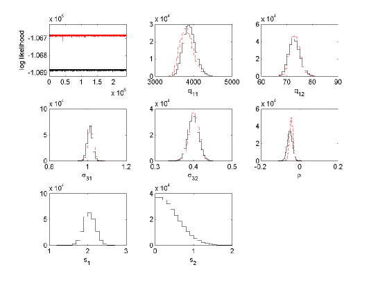
Figure 1: Results from run done with training data ${\bf D}$ with the $nonnested-GP$ model, are shown in grey (or red in the electronic version), while results from run undertaken with training and test data, $\boldsymbol{D}^{\star}$, in this $nonnested-GP$ model, are depicted in black. Traces of the logarithm of the likelihood are displayed from the two runs in the top left panel. Reciprocal of the length scale parameters are the shown in the top middle and right panels; here $q_{c}=\ell_{c}^{-1},\>c=1,2$. Histograms representing marginal posterior probability density of the learnt diagonal elements $\sigma_{11}^{(1)}$ and $\sigma_{22}^{(1)}$, of the covariance matrix $\boldsymbol{\Sigma}_{1}$, are shown in the mid-row, left and middle panels (given respective data). Histograms representing marginals of the parameter $\rho=\displaystyle{\frac{\sigma_{12}}{\sqrt{\sigma_{11}^{(1)}\sigma_{22}^{(1)}}}}$ are displayed in the mid-row right panel. Prediction of the values of the input parameter $\boldsymbol{S}=(S_{1},S_{2})^{T}$ is possible only in the run performed with both training and test data. Marginals of $S_{1}$ and $S_{2}$ values learnt via MCMC-based sampling from the joint of all unknown parameters given $\boldsymbol{D}^{\star}$, are shown in the lower panel, as approximated by histograms.

7 Results

In this section, we present the results of learning the unknown parameters of the 3rd-order tensor-normal likelihood, given the training as well as the training+test data.

While Figure 1 of the Supplementary Materials and Figure 1 here depict results obtained from using the $nonnested-GP$, in the following figures, results of the learning of all relevant unknown parameters, using the $nested-GP$ model, are included. Figures that depict results from the $nested-GP$ approach will include results of the learning of amplitude $a_{c}$ and smoothing parameters $d_{c}:=1/\delta_{c}$ parameters. Also, our modelling under the $nested-GP$ paradigm relies on a lookback-time $t_{0}$ which gives the number of iterations over which we gather the generated $\ell_{c}$ values.

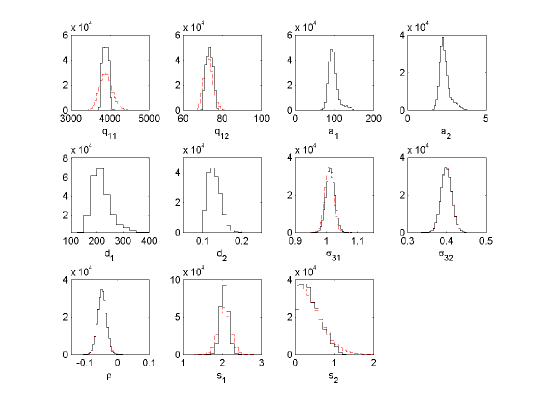
Figure 2: Results from run done with test+training data ${\boldsymbol{D}}^{\star}$ within the $nested-GP$ model, shown in black, as distinguished from the results of learning given the same data, and the $nonnested-GP$ model depicted in grey (or red in the electronic copy of the thesis). Here the used value of $T_{0}$ is 200 iterations. Histograms approximating the marginal posterior probability densities of each sought unknown is depicted. Here, sought hyperparameter values $a_{c}$ and $\delta_{c}$ are relevant only to the $nested-GP$ model ($c=1,2$). Here, we have undertaken sampling from the joint posterior of all parameters, including the input parameter values $s_{1}^{(test)}$ and $s_{2}^{(test)}$, at which the test data are realised. Histograms approximating marginal posterior of each learnt unknown are presented.

.

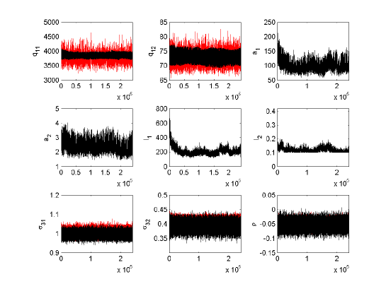
Figure 3: Traces of parameters learnt using the training data ${\bf D}$, in the run performed with the $nonnested-GP$ model, are compared to traces of the corresponding parameter obtained in the run performed with the $nested-GP$ model. Traces of parameters learnt within the $nonnested-GP$ model are in grey (or red in the e-version) while the traces obtained using the $nested-GP$ model are shown in black.

.

7.1 Effect of discontinuity in the data, manifest in our results

One difference between the learning of parameters from the $nested-GP$, as distinguished from the $nonnested-GP$ models is the quality of the inference, in the sense that the uncertainty of parameters (i.e. the 95$\%$ HPDs) learnt using the $nested-GP$ models, is less than that learnt using the $nonnested-GP$ models. This difference in the learnt HPDs is most marked for the learning of values of $Q_{1}$ and $S_{1}$, and $S_{2}$ to a lesser extent.

We explain this, by invoking the discontinuity in the training data–distribution of $S_{1}$ in this data is sharply discontinuous, though there is a less sharp discontinuity in the distribution of $S_{2}$ noted. We refer to Figure 8 of Chakrabarty (2007), page 152. This figure is available at https://www.aanda.org/articles/aa/pdf/2007/19/aa6677-06.pdf, and corresponds to the base astronomical model used in the simulations that generate the training data that we use here. This figure informs on the distribution of location $\boldsymbol{S}$; compatibility of the stellar velocity matrix $\boldsymbol{v}(=\boldsymbol{\xi}(\boldsymbol{s}))$ realised (in astronomical simulations) at a given $\boldsymbol{s}$, to the test velocity matrix $\boldsymbol{v}^{(test)}$ (recorded by the Hipparcos satellite), is parametrised, and this compatibility parameter plotted against $\boldsymbol{s}$ in this figure. In fact, this figure is a contour plot of the distribution of such a compatibility parameter, in the space ${\cal D}$, where $\boldsymbol{S}\in{\cal D}\subset{\mathbb{R}}^{2}$. The 2 components of $\boldsymbol{S}$ are represented in polar coordinates, with $S_{1}$ the radial and $S_{2}$ the angular component. We see clearly from this figure, that the distribution across $S_{1}$ is highly discontinuous, at given values of $S_{2}$ (i.e. at fixed angular bins). In fact, this distribution is visually more discontinuous, than the distribution across $S_{2}$, at given values of $S_{1}$, i.e. at fixed radial bins (each of which is represented by the space between two bounding radial arcs). In other words, the velocity matrices that are astronomically simulated at different $\boldsymbol{S}$ values, are differently compatible with a given reference velocity matrix ($\boldsymbol{v}^{(test)}$)–and, the distribution of velocity matrix variable $\boldsymbol{V}$, is discontinuous across values of $\boldsymbol{S}$, and in fact, less smoothly distributed at fixed $s_{2}$, than at fixed $s_{1}$. Thus, this figure brings forth the discontinuity with the input-space variable $\boldsymbol{S}$, in the data tensor $\boldsymbol{D}_{\boldsymbol{V}}$ that is part of the training data.

Then, it is incorrect to use a stationary kernel to parametrise the covariance $\boldsymbol{\Sigma}_{3}$, that informs on the covariance between velocity matrices generated at different values of $\boldsymbol{S}$. Our implementation of the $nested-GP$ model tackles this shortcoming of the model. However, when we implement the $nonnested-GP$ model, Metropolis needs to explore a wider volume of the state space to accommodate parameter values, given the data at hand–and even then, there is a possibility for incorrect inference under the stationary kernel model. This explains the noted trend of higher 95$\%$ HPDs on most parameters learnt using the $nonnested-GP$ model, compared to the $nested-GP$ model, as observed in comparison of results from runs done with training data alone, or both training and test data; compare Figure 2 to Figure 3, and note the comparison in the traces as displayed in Figure 3. Indeed, this also explains the bigger difference noted in these figures when we compare the learning of $q_{1}$ over $q_{2}$, in runs that use the stationary model, as distinguished from the non-stationary model. After all, the discontinuity across $S_{1}$ is discussed above, to be higher than across $S_{2}$.

7.2 Effect of varying lookback times, i.e. length of historical data

To check for the effect of the lookback time $t_{0}$, we present traces of the covariance parameters and kernel hyperparameters learnt from runs undertaken within the $nested-GP$ model, but different $t_{0}$ values of 50 and 100, in Figure 4, which we can compare to the traces obtained in runs performed under the $nested-GP$ model, with $t_{0}=200$, as displayed in Figure 3.

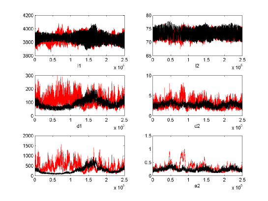
Figure 4: Comparison of traces of unknown smoothness parameters of $\boldsymbol{\Sigma}_{3}$ and hyperparameters of GPs invoked to model these parameters, obtained in runs performed with training data ${\bf D}$ and $t_{0}=50$ (in grey, or red in the e-version) and $t_{0}=100$ (in black).

.

It is indeed interesting to note the trends in traces of the the smoothness parameters $q$ that are the reciprocal of $\ell$ parameters, and values of the amplitude ($a_{1},a_{2}$) and values of length scale hyperparameters ($\delta_{1},\delta_{2}$), evidenced in Figure 4 and the results in black in Figure 3). A zeroth-order model for these parameters that are realisations from a non-stationary process, is a moving averages time-series model–$MA(t_{0})$ to be precise. We note the increase in fluctuation amplitude of the traces, with decreasing $t_{0}$. For smaller values of lookback time $t_{0}$, the average covariance between $g_{\boldsymbol{x}_{c}}(t_{1})$ and $g_{\boldsymbol{x}_{c}}(t_{2})$ is higher, than when $t_{0}$ is higher, where the averaging is performed over a $t_{0}$-iteration long interval that has its right edge on the current iteration; here $\boldsymbol{x}_{c}=(a_{c},\delta_{c})^{T}$, $c=1,2$ and as introduced above, we model the length scale parameter of the kernel that parametrises $\boldsymbol{\Sigma}_{3}$, as $\ell_{c}=g_{\boldsymbol{x}_{c}}(t)$. Here $g_{\boldsymbol{x}_{c}}(\cdot)$ is modelled as a realisation from a scalar-variate GP with covariance kernel that is itself kernel-parametrised using an SQE kernel with amplitude $a_{c}$ and correlation-length $\delta_{c}$. Then higher covariances between values of $g_{\boldsymbol{x}_{c}}(\cdot)$ at different $t$-values in general would suggest higher values of the global amplitude of this parametrised kernel, and higher values of the length-scales of this SQE kernel.

Indeed an important question is, what is the “best” $t_{0}$, given our data. Such question is itself of relevance, and discussed intensively under distributed lag models, often within Econometrics (Shirley, 1965). An interesting trend noted in the parameter traces presented in Figure 4 for $t_{0}=50,100$, and to a lesser extent for $t_{0}=200$, in the results in black in Figure 3, is the global near-periodic existence of crests and troughs in these traces. This periodic fluctuation is more marked for smoothness $q_{1}$ (=$1/\ell_{1}$) and the hyperparameters of the scalar-variate GP used to model $g_{\boldsymbol{x}_{1}}(\cdot)$, than for $q_{2}$ (and $a_{2}$ and $\delta_{2}$).

From the point of view of a polynomial (of order $t_{0}$) model for the lag operator–that transfers information from the past $t_{0}$ realisations from a stochastic process to the current iteration–the shape of the trace will be dictated by parameters of ths model. If this polynomial admits complex roots, then coefficients of the relevant lag terms will behave like a damped sine function with iterations. For a different value of $t_{0}$, such a pronounced oscillatory trend might not be equally apparent. Loosely speaking, the value of $\ell_{c}$ in any iteration, represented by a moving average, will manifest the result of superposition of the different (discontinuous) modal neighbourhoods present in the data. The more multimodal the data, i.e. larger the number of “classes” (by correlation-length scales) of functional form $\boldsymbol{\xi}(\cdot)$ sampled from the tensor-variate GP, s.t. superposition of the sample paths will cause a washing-out of the effect of the different modes, and a less prominent global trend will be manifest in the traces. However, for data that is globally bimodal, the superposition of the two “classes” of sampled functions $\boldsymbol{\xi}(\cdot)$ will create a periodicity in the global trend of the generated $\ell_{c}$ values (and thereby of the smoothness parameter values $q_{c}$, where $q=\ell_{c}^{-1}$). Again, the larger the value $t_{0}$ of the lookback-time parameter, the moving average is over a larger number of samples, and hence greater is the washing-out effect. Thus, depending on the discontinuity in the data, it is anticipated that there is a range of optimal lookback-time values, for which, the global periodicity is most marked. This is what we might be noticing in the trace of $q_{1}$ at $t_{0}=100$ displaying the global periodicity more strongly than that at $t_{0}=200$ (see Figure 4 and Figure 3).

Another point is that the strength of this global periodicity will be stronger for the correlation-length scale along that direction in input-space, the discontinuity along which is stronger. Indeed, as we have discussed above, the discontinuity in the data with varying $S_{1}$ is anticipated to be higher than with $S_{2}$. So we would expect a more prominent periodic trend in the trace of $q_{1}$ than $q_{2}$. This is indeed what to note in Figure 4. A simulation study can be undertaken to explore the effects of empirical discontinuities.

The arguments above qualitatively explain the observed trends in the traces of the hyperparameters, obtained from runs using different $t_{0}$. That in spite of discrepancies in $a_{c}$ and $\delta_{c}$, with $t_{0}$, values of the length scale parameter $\ell_{c}$ (and therefore its reciprocal $q_{c}$) are concurrent within the 95$\%$ HPDs, is testament to the robustness of inference. Stationarity of the traces betrays the achievement of convergence of the chain.

We notice that the reciprocal correlation length scale $q_{1}$ is a couple of orders of magnitude higher than $q_{2}$; correlation between values of the sampled function $\boldsymbol{\xi}(\cdot)$, at 2 different $S_{1}$ values (at the same $s_{2}$), then wanes more quickly than correlation between sampled functions computed at same $s_{1}$ and different $S_{2}$ values. Here $\boldsymbol{s}=(s_{1},s_{2})^{T}$ and given that $\boldsymbol{S}$ is the location of the observer who observes the velocities of her neighbouring stars on a two-dimensional polar grid, $S_{1}$ is interpreted as the radial coordinate of the observer’s location in the Galaxy and $S_{2}$ is the observer’s angular coordinate. Then it appears that the velocities measured by observers at different radial coordinates, but at the same angle, are correlated over shorter radial-length scales than velocities measured by observers at the same radial coordinate, but different angles. This is understood to be due to the astro-dynamical influences of the Galactic features included by Chakrabarty (2007) in the simulation that generates the training data that we use here. This simulation incorporates the joint dynamical effect of the Galactic spiral arms and the elongated Galactic bar (made of stars) that rotate at different frequencies (as per the astronomical model responsible for the generation of our training data), pivoted at the centre of the Galaxy. An effect of this joint handiwork of the bar and the spiral arms is to generate distinctive stellar velocity distributions at different radial (i.e. along the $S_{1}$ direction) coordinates, at the same angle ($s_{2}$). On the other hand, the stellar velocity distributions are more similar at different $S_{2}$ values, at the same $s_{1}$. This pattern is borne by the work by Chakrabarty (2004), in which the radial and angular variation of the standard deviations of these bivariate velocity distributions are plotted. Then it is understandable why the correlation length scales are shorter along the $S_{1}$ direction, than along the $S_{2}$ direction.

Furthermore, for the correlation parameter $\rho$, physics suggests that the correlation will be zero among the two components of a velocity vector. These two components are after all, the components of the velocity vector in a 2-dimensional orthogonal basis. However, the MCMC chain shows that there is a small (negative) correlation between the two components of the stellar velocity vector.

7.3 Predicting $\boldsymbol{s}^{(test)}$

Figure 1, displays histogram-representations of marginal posterior probability densities of the solar location coordinates $s^{(test)}_{1}$, $s^{(test)}_{2}$; $q_{1}^{*}$ and $q_{2}^{*}$ that get updated once the test data is added to augment the training data, and parameters $\sigma_{11}^{1*}$, $\sigma_{22}^{1*}$ and $\rho^{*}$. 95$\%$ HPD credible regions computed on each parameter in this inference scheme, are displayed in Table 1 of Supplementary Materials. These figures display these parameters in the $nonnested-GP$ model. When the $nested-GP$ model is used, histogram-representations of the marginals of the aforementioned parameters, are displayed in Figure 2.

Prediction of $\boldsymbol{s}^{(test)}$ using the $nested-GP$ models gives rise to similar results as when the $nonnested-GP$ models are used, (see Figure 2 that compares the marginals of the solar location parameters sampled from the joint of all unknowns, given all data, in $nested-GP$ models, against those obtained when $nonnested-GP$ models are used).

The marginal distributions of $s_{1}^{(test)}$ indicates that the marginal is unimodal and converges well, with modes at about 2 in model units. The distribution of $s_{2}^{(test)}$ on the other hand is quite strongly skewed towards values of $s_{2}^{(test)}\lesssim 1$ radians, i.e. $s_{2}^{(test)}\lesssim 57$ degrees, though the probability mass in this marginal density falls sharply after about 0.4 radians, i.e. about 23 degrees. These values tally quite well with previous work (Chakrabarty et al., 2015). In that earlier work, using the training data that we use in this work, (constructed using the the astronomical model $sp3bar3{\_}18$ discussed by Chakrabarty et al. (2015)), the marginal distribution of $s_{1}^{(test)}$ was learnt to be bimodal, with modes at about 1.85 and 2, in model units. The distribution of $s_{2}^{(test)}$ found by Chakrabarty et al. (2015) is however more constricted, with a sharp mode at about 0.32 radians (i.e. about 20 degrees). We do notice a mode at about this value in our inference, but unlike in the results of Chakrabarty et al. (2015), we do not find the probability mass declining to low values beyond about 15 degrees. One possible reason for this lack of compatibility could be that in Chakrabarty et al. (2015), the matrix of velocities $\boldsymbol{V}$ was vectorised, so that the training data then resembled a matrix, rather than a 3-tensor as we know it to be. Such vectorisation could have led to some loss of correlation information, leading to their results.

Model checking of our models and results is undertaken in Section 3 of the Supplementary Materials.

7.4 Astronomical implications

The radial coordinate of the observer in the Milky Way, i.e. the solar radial location, is dealt with in model units, but will need to be scaled to real galactic unit of distance, which is kilo parsec (kpc). Now, from independent astronomical work, the radial location of the Sun is set as 8 kpc. Then our learnt value of $S_{1}^{(test)}$ is to be scaled to 8 kpc, which gives 1 model unit of length to be ${{m}}:=\displaystyle{\left(\frac{8\mbox{kpc}}{\mbox{learnt value of\>\>}S_{1}^{(test)}}\right)}$. Our main interest in learning the solar location is to find the frequency $\Omega_{bar}$ with which the Galactic bar is rotating, pivoted at the galactic centre, (loosely speaking). Here $\Omega_{bar}=\displaystyle{\frac{v_{0}}{\mbox{1 model unit of length}}=\frac{v_{0}}{{m}}}$, where $v_{0}=220$ km/s (see Chakrabarty (2007) for details). The solar angular location being measured as the angular distance from the long-axis of the Galactic bar, our estimate of $S_{2}$ actually tells us the angular distance between the Sun-Galactic centre line and the long axis of the bar. These estimates are included in Table 1.

Table 1: $95\%$ HPD on each Galactic feature parameter learnt from the solar location coordinates learnt using the two predictive inference schemes listed above and as reported in a past paper for the same training and test data.

	$95\%$ HPD for $\Omega_{bar}$ (km/s/kpc)	for angular distance of
		bar to Sun (degrees)
from posterior predictive	$[48.11,57.73]$	$[4.53,43.62]$
from joint posterior	$[48.25,57.244]$	$[2.25,46.80]$
from Chakrabarty et. al (2015)	$[46.75,62.98]$	$[17.60,79.90]$

Table 1 displays the Galactic feature parameters that are derived from the learnt solar location parameters, under the different inference schemes using the $nonnested-GP$ model, namely, sampling from the joint posterior probability of all parameters given all data, and from the posterior predictive of the solar location coordinates given test data and GP parameters already learnt from training data alone. The derived Galactic feature parameters are the bar rotational frequency $\Omega_{bar}$ in the real astronomical units of km/s/kpc and the angular distance between the bar and the Sun, in degrees. The table also includes results from Chakrabarty et al. (2015), the reference for which is in the main paper.

8 Conclusions

Our work presents a method for learning tensor-valued functional relations between a sytem parameter vector, and a tensor-valued observable, multiple measurements of which build up a hypercuboidally-shaped data, that is in general not continuous, thus demanding a non-stationary covariance structure of the invoked GP. We clarify the need for generalising a stationary covariance to one in which the hyperparameters (correlation length scales along each direction of the space of the system parameter vector) need to be treated as dependent on the sample function of the invoked GP. We address this need by modelling the sought tensor-valued function with a tensor-variate GP, each parameter of the covariance function of which, is modelled as a dynamically varying, scalar-valued function that is treated as a realisation from a scalar-variate GP with distinct covariance structure, that we parametrise. We employ Metropolis-within-Gibbs-based inference, that allows comprehensive and objective uncertainties on all learnt unknowns. Subsequent to the learning of the sought tensor-valued function, we make an inverse Bayesian prediction of the system parameter values at which test data on the observable is realised. While in this work we focussed on the learning given discontinuous data, the inclusion of non-stationarity in the covariance is a generic cure for non-stationary data; we will consider an application to a temporally varying, econometric dataset in a future contribution.

, t2PhD student in Department of Mathematics, University of Leicester t1Lecturer in Statistics, Department of Mathematical Sciences, Loughborough University

Here, we refer to the main paper as “KWDC”.

9 Algorithm used to make inference in KWDC

1. In the $0$-th iteration, set all unknown parameters to arbitrarily chosen seed values : $a_{c}$ is set to the seed $a_{c}^{(0)}$ and $\delta_{c}$ is set to the seed $\delta_{c}^{(0)}$ $\forall c=1,\ldots,d$; $\sigma_{q}$ is set to the seed $\sigma_{q}^{(0)}$ $\forall q=1,\ldots,q_{max}$. We also set the length scales of the kernel-parametrised covariance matrix $\boldsymbol{\Sigma}_{p}$ to their respective seed values, i.e. set $\ell_{c}:=\ell_{c}^{(0)}\forall c=1,\ldots,d$.

2. At the beginning of the $t$-th iteration, for $t<t_{0}$, the current value of the $ell_{c}$ parameter is $\ell_{c}^{(t-1)}$. We propose the new value, $\ell_{c}^{(t\star)}$ from a Gaussian distribution, the mean of which is the current value of this parameter, namely $\ell_{c}^{(t-1)}$, and the variance of which is chosen experimentally, to be the constant $v_{c}$, i.e.

   $$\ell_{c}^{(t\star)}\sim{\cal N}(\ell_{c}^{(t-1)},v_{c}).$$

   This proposing is undertaken $\forall c=1,\ldots,d$. We choose adequate priors (often Gaussian priors with mean $\ell_{c}^{(0)}$ and large constant variances) on all the $\ell_{c}$ parameters. We refer to these priors as $pi_{0}(\ell_{1},\ldots,\ell_{d})$. The proposed $\ell_{c}$ parameters then inform the kernel function $K_{p}(\cdot,\cdot)$ that is used to kernel parametrise the covariance matrix $\boldsymbol{\Sigma}_{p}$, s.t. the proposed kernel-parametrised covariance matrix in the $t$-th iteration, $t<t_{0}$, is $\boldsymbol{\Sigma}_{p}^{(t\star)}=\boldsymbol{A}_{p}^{(t\star)}(\boldsymbol{A}_{p}^{(t\star)})^{T}$, while the current values of the $\ell_{c}$ parameters suggest that the current kernel-parametrised covariance matrix is $\boldsymbol{\Sigma}_{p}^{(t-1)}=\boldsymbol{A}_{p}^{(t-1)}(\boldsymbol{A}_{p}^{(t-1)})^{T}$. We compute $\boldsymbol{\Sigma}_{p}^{(t\star)}=\left[\exp\left(-\frac{(\boldsymbol{s}_{i}-\boldsymbol{s}_{j})^{2}}{2(\boldsymbol{\ell}^{(t\star)})^{2}}\right)\right]$, where $\boldsymbol{\ell}^{(t\star)}:=(\ell_{1}^{(t\star)},\ldots,\ell_{d}^{(t\star)})^{T}$. Similarly, $\boldsymbol{\Sigma}_{p}^{(t-1)}$ is defined in terms of the vector of the length scales, $\boldsymbol{\ell}^{(t-1)}$ that is the current value of the end of the $t-1$-th iteration.

3. We compute the ratio of the posterior probability densities of the proposed $\ell_{c}$ parameters given the training data ${\bf D}$ to the posterior of the current $\ell_{c}$ values. The ratio of the proposal densities does not get invoked since the proposal is symmetric. Thus, the ratio that we compute is

   $$r:=\displaystyle{\frac{\exp(-\|({\bf D})\times_{1}\boldsymbol{A}_{1}^{-1}\ldots\times_{p}(\boldsymbol{A}_{p}^{(t\star)})^{-1}\ldots\times_{k}\boldsymbol{A}_{k}^{-1}\|^{2}/2)\pi_{0}(\ell_{1}^{(t\star)},\ldots,\ell_{d}^{(t\star)})}{\exp(-\|({\bf D})\times_{1}\boldsymbol{A}_{1}^{-1}\ldots\times_{p}(\boldsymbol{A}_{p}^{(t-1)})^{-1}\ldots\times_{k}\boldsymbol{A}_{k}^{-1}\|^{2}/2)\pi_{0}(\ell_{1}^{(t-1)},\ldots,\ell_{d}^{(t-1)})}},$$

   and compare $r$ with the value of the uniform random variate $U\sim{\cal U}[0,1]$.
   –If $u\geq r$, we reject the proposed values $\ell_{1}^{(t\star)},\ldots,\ell_{d}^{(t\star)}$, and set the current value of the $\ell_{c}$ parameter at the end of the $t$-th iteration to be $\ell_{c}^{(t)}=\ell_{c}^{(t-1)}\forall c=1,\ldots,d$.
   –If $u<r$, we accept the proposed values $\ell_{1}^{(t\star)},\ldots,\ell_{d}^{(t\star)}$, and set the current value of the $\ell_{c}$ parameter at the end of the $t$-th iteration to be $\ell_{c}^{(t)}=\ell_{c}^{(t\star)},\forall c=1,\ldots,d$.
   Thus, for iterations $t<t_{0}$, the first block update is a manifestation of Random Walk.

4. If the iteration number $t$ is s.t. $t\geq t_{0}$, then we model the $\ell_{c}$ parameters, each as a realisation from a distinct scalar-variate GP, the covariance structure of which is kernel-parametrised s.t. these kernel hyperparameters are $a_{c}$ and $\delta_{c}$, $\forall c=1,\ldots,d$. Then the counterpart of point 2(a), within the “nested GP” approach, is now discussed. Let the current values of $a_{c}$ and $\delta_{c}$ be $a_{c}^{(t-1)}$ and $\delta_{c}^{(t-1)}$. We propose values of these parameters in the $t$-th iteration, respectively from a Truncated-Normal density (left-truncated at 0, mean $a_{c}^{(t-1)}$, and experimentally chosen constant variance $v_{a}^{(c)}$), and a Normal (mean $\delta_{c}^{(t-1)}$, and experimentally chosen constant variance $v_{\delta}^{(c)}$), i.e.

   $$a_{c}^{(t\star)}\sim{\cal TN}(a_{c}^{(t-1)},0,v_{a}^{(c)}),\quad\forall c=1,\ldots,d,$$

   $$\delta_{c}^{(t\star)}\sim{\cal N}(\delta_{c}^{(t-1)},0,v_{\delta}^{(c)}),\quad\forall c=1,\ldots,d.$$

   Now the GP that $\ell_{c}$ is modelled with, currently has a covariance structure that is parametrised by the $t_{0}\times t_{0}$-dimensional covariance matrix $\boldsymbol{S}_{c}$ s.t. currently the $ij$-th element of this matrix is the covariance between the value of $\ell_{c}$ that was current in the $t-i$-th iteration and the value current in the $t-j$-th iteration, i.e. $\boldsymbol{S}_{c}^{(t-1)}=\left[a_{c}^{(t-1)}\exp\left(-\frac{(i-j)^{2}}{2(\delta_{c}^{(t-1)})^{2}}\right)\right]$; $i,j=1,\ldots,t_{0}$. Thus, at any fixed value (say $i$) of the input variable–the iteration number–the $i$-th diagonal element $a_{c}^{(t-i)}$ of the covariance matrix $\boldsymbol{S}$, gives the variance of the Gaussian distribution that $\ell_{c}^{(t-i)}$ can be considered to be sampled from. Following this, we reduce this scalar-variate GP to a Gaussian distribution, by fixing the value of the input-space variable, (which in this situation is the iteration number), to $t$. Then the proposed variance of the Gaussian distribution that $\ell_{c}$ is sampled from, at the $t$-th iteration, is the proposed value of the $a_{c}$ parameter in this iteration, i.e. $a_{c}^{(t\star)}$. Under a Random Walk paradigm, the mean of this Gaussian distribution is the current value of the $\ell_{c}$ parameter. In other words, the model suggests that

   $$\ell_{c}^{t\star}\sim{\cal N}(\ell_{c}^{(t-1)},a_{c}^{(t\star)}).$$

   This is essentially suggesting an adaptive Random Walk updating scheme for the $\ell_{c}$ parameter, $\forall c=1,\ldots,d$.

5. This is the counterpart of point 3(a) for the $t\geq t_{0}$ iterations, i.e. when the “nested GP” model is in play. Again, as during the discussion of 3(a), here we compute the ratio of the posterior probability densities of the proposed to the current values of the unknowns that are updated in the first block. This posterior has the contribution from the $k$-th ordered tensor-normal likelihood that the observable $\boldsymbol{V}$ ($=\boldsymbol{\xi}(\boldsymbol{S})$) is modelled as a realisation from. But the covariance matrix $\boldsymbol{\Sigma}_{p}$ of this tensor-normal likelihood is kernel-parametrised, with a GP prior imposed on each length scale parameters $\ell_{1},\ldots,\ell_{d}$ of this kernel function. Then the joint probability density of the set of $t_{0}$ number of realisations $\{\ell_{c}^{(t-t_{0})},\ldots,\ell_{c}^{(t-1)}\}$ of the parameter $\ell_{c}$, from the scalar-variate, zero-mean GP, is multivariate normal with mean vector ${\bf 0}$ and covariance matrix $\boldsymbol{S}_{c}=[s_{c}^{(ij)}]$, which is kernel-parametrised as $s_{c}^{ij}=\displaystyle{a_{c}\exp\left[-\frac{(i-j)^{2}}{2\delta_{c}^{2}}\right]}$, s.t. the current value of the covariance matrix in the $t$-th iteration is $\boldsymbol{S}_{c}^{(t-1)}=\displaystyle{\left[{a_{c}^{(t-1)}\exp\left[-\frac{(i-j)^{2}}{2(\delta_{c}^{(t-1)})^{2}}\right]}\right]}$, and the proposed value of the covariance matrix in the $t$-th iteration is $\boldsymbol{S}_{c}^{(t\star)}=\displaystyle{\left[{a_{c}^{(t\star)}\exp\left[-\frac{(i-j)^{2}}{2(\delta_{c}^{(t\star)})^{2}}\right]}\right]}$. In other words, the prior probability density on the $t_{0}$-dimensional vector $\boldsymbol{\ell}_{c}^{(t_{0})}:=(\ell_{c}^{(t-t_{0})},\ldots,\ell_{c}^{(t-1)})^{T}$ of values of the $c$-th length scale parameter, over the last $t_{0}$ iterations is multivariate normal, with mean vector ${\bf 0}$ and covariance matrix $\boldsymbol{S}$, i.e.

   $$\pi_{0}(\ell_{c}^{(t-t_{0})},\ldots,\ell_{c}^{(t-1)})=\displaystyle{\frac{1}{\sqrt{\det(2\pi\boldsymbol{S})}}\exp\left[-\frac{1}{2}(\boldsymbol{\ell}_{c}^{(t_{0})})^{T}\boldsymbol{S}^{-1}(\boldsymbol{\ell}_{c}^{(t_{0})})\right]},$$

   where $\boldsymbol{\ell}_{c}^{(t_{0})}$ and the current and proposed $\boldsymbol{S}$ (as a function of current and proposed $a_{c}$ and $\delta_{c}$ values) are defined above. This is true $\forall c=1,\ldots,d$. Then the ratio of the posterior probability density of the proposed to the current values of the unknowns $a_{1},\ldots,a_{d},\delta_{1},\ldots,\delta_{c}$, given the data is

   $$r:=\displaystyle{\frac{\exp(-\|({\bf D})\times_{1}\boldsymbol{A}_{1}^{-1}\ldots\times_{p}(\boldsymbol{A}_{p}^{(t\star)})^{-1}\ldots\times_{k}\boldsymbol{A}_{k}^{-1}\|^{2}/2)\prod\limits_{c=1}^{d}\frac{1}{\sqrt{\det(2\pi\boldsymbol{S}^{(t\star)})}}\exp\left[-\frac{1}{2}(\boldsymbol{\ell}_{c}^{(t_{0})})^{T}(\boldsymbol{S}^{(t\star)}){-1}(\boldsymbol{\ell}_{c}^{(t_{0})})\right]\prod\limits_{c=1}^{d}{\cal TN}(a_{c}^{(t\star)},0,v_{a}^{(c)})}{\exp(-\|({\bf D})\times_{1}\boldsymbol{A}_{1}^{-1}\ldots\times_{p}(\boldsymbol{A}_{p}^{(t-1)})^{-1}\ldots\times_{k}\boldsymbol{A}_{k}^{-1}\|^{2}/2)\prod\limits_{c=1}^{d}\frac{1}{\sqrt{\det(2\pi\boldsymbol{S}^{(t-1)})}}\exp\left[-\frac{1}{2}(\boldsymbol{\ell}_{c}^{(t_{0})})^{T}(\boldsymbol{S}^{(t-1)}){-1}(\boldsymbol{\ell}_{c}^{(t_{0})})\right]\prod\limits_{c=1}^{d}{\cal TN}(a_{c}^{(t-1)},0,v_{a}^{(c)})}},$$

   and compare $r$ with the value of the uniform random variate $U\sim{\cal U}[0,1]$.
   –If $u\geq r$, we reject the proposed values of the unknowns, and set the current value of the $\delta_{c}$ and $a_{c}$ parameters at the end of the $t$-th iteration to be $a_{c}^{(t)}=a_{c}^{(t-1)},\delta_{c}^{(t)}=\delta_{c}^{(t-1)},\forall c=1,\ldots,d$.
   –If $u<r$, we accept the proposed values, and set $a_{c}^{(t)}=a_{c}^{(t\star)},\delta_{c}^{(t)}=\delta_{c}^{(t\star)},\forall c=1,\ldots,d$.
   Thus, the updating for the $\delta_{c}$ parameters is Random Walk as they are proposed from a Gaussian.

6. In this point, we discuss the updating of the remaining unknowns, $\sigma_{1},\ldots,\sigma_{q_{max}}$, i.e. the elements of covariance matrices of the tensor-normal joint probability distribution of a set of realisations of $\boldsymbol{V}$ ($=\boldsymbol{\xi}(\boldsymbol{S})$), that are not kernel-parametrised, but learnt directly by MCMC. These elements can in general be positive of negative, and so, in the $t$-th iteration, we propose them from a Gaussian with mean given by their current value $\sigma_{q}^{(t-1)}$, and experimentally fixed variance $v_{q}$, $q=1,\ldots,q_{max}$, i.e. the proposed value is

   $$\sigma_{q}^{(t\star)}\sim{\cal N}(\sigma_{q}^{(t-1)},v_{q})\quad\forall q=1,\ldots,v_{q}.$$

   Then using these proposed values of the elements, the proposed values of all covariance matrices other than $\boldsymbol{\Sigma}_{p}$ that is kernel-parametrised, are $\boldsymbol{\Sigma}_{1}^{(t\star)},\ldots,\boldsymbol{\Sigma}_{p-1}^{(t\star)},\boldsymbol{\Sigma}_{p+1}^{(t\star)},\ldots,\boldsymbol{\Sigma}_{k}^{(t\star)}$, while their current values (populated by the current values $\sigma_{q}^{(t-1)}$ of elements) are $\boldsymbol{\Sigma}_{1}^{(t-1)},\ldots,\boldsymbol{\Sigma}_{p-1}^{(t-1)},\boldsymbol{\Sigma}_{p+1}^{(t-1)},\ldots,\boldsymbol{\Sigma}_{k}^{(t-1)}$. The priors on the $\sigma_{q}$ parameters are treated as Gaussians with mean given by the seed value of $\sigma_{q}^{(0)}$ and experimentally chose, large variance, to suggest vague priors. Thus, the ratio of the posterior probability of the proposed and current $\sigma_{1},\ldots,\sigma_{q_{max}}$, parameters, given the training data ${\bf D}$, at the already updated $\boldsymbol{\Sigma}_{p}$ to value $\boldsymbol{\Sigma}_{p}^{(t)}=(A_{p}^{(t)})^{T}A_{p}^{(t)}$, is

   $$r:=\displaystyle{\frac{\exp(-\|({\bf D})\times_{1}(\boldsymbol{A}_{1}^{(t\star)}){-1}\ldots\times_{p-1}(\boldsymbol{A}_{p-1}^{(t\star)})^{-1}\times_{p}(\boldsymbol{A}_{p}^{(t)})^{-1}\times_{p+1}(\boldsymbol{A}_{p+1}^{(t\star)})^{-1}\ldots\times_{k}(\boldsymbol{A}_{k}{(t\star)})^{-1}\|^{2}/2)\pi_{0}(\sigma_{1}^{(t\star)},\ldots,\sigma_{q_{max}}^{(t\star)})}{\exp(-\|({\bf D})\times_{1}(\boldsymbol{A}_{1}^{(t-1)}){-1}\ldots\times_{p-1}(\boldsymbol{A}_{p-1}^{(t-1)})^{-1}\times_{p}(\boldsymbol{A}_{p}^{(t\star)})^{-1}\times_{p+1}(\boldsymbol{A}_{p+1}^{(t-1)})^{-1}\ldots\times_{k}(\boldsymbol{A}_{k}{(t-1)})^{-1}\|^{2}/2)\pi_{0}(\sigma_{1}^{(t-1)},\ldots,\sigma_{q_{max}}^{(t-1)})}},$$

   and compare $r$ with the value of the uniform random variate $U\sim{\cal U}[0,1]$.
   It is possible that some of these $k-1$ covariance matrices are not learnt using MCMC, but empirically estimated–in that case, the empirically estimated value of the corresponding covariance matrix is used in both denominator and numerator in the definition of the likelihood above, instead of its current and proposed values respectively. –If $u\geq r$, we reject the proposed values of the unknowns, and set the current value of the $\sigma_{q}$ at the end of the $t$-th iteration to be $\sigma_{q}^{(t)}=\sigma_{q}^{(t-1)},\forall q=1,\ldots,q_{max}$.
   –If $u<r$, we accept the proposed values, and set $\sigma_{q}^{(t)}=\sigma_{q}^{(t\star)},\forall q=1,\ldots,q_{max}$.
   Thus, the updating for the $\sigma_{q}$ parameters is Random Walk as they are proposed from a Gaussian.

7. Repeat steps 2-5 until $t=t_{max}$, the length of the chain.

10 Results

Figure 5 display traces of the sought parameters learnt using the $nonnested-GP$. In the following figure (Figure 6), marginal posterior probability density of the sought parameters, given training data, (depicted as histograms), obtained using the $nonnoested-GP$ model, are compared to the corresponding result obtained from the $nested-GP$ model. In this $nested-GP$ model, the covariance matrix $\boldsymbol{\Sigma}_{3}$ (that bears information about the covariance structure between sheets of data generated at different values of the input variable $\boldsymbol{S}=(S_{1},S_{2})^{T}$), is parameterised using a kernel, each length-scale hyperparameter of which, is itself modelled as a dynamically-varying function that is considered sampled from a GP. For each such scalar-variate GP that generates the length-scale $\ell_{c}$, $c=1,\ldots,d=2$ the covariance matrix is itself kernel-parametrised using a stationary kernel, with an amplitude parameter value $a_{c}$ and length-scale parameter $\delta_{c}$.

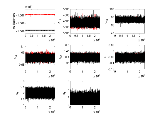
Figure 5: Results from run done with training data ${\bf D}$ with the $nonnested-GP$ model, are shown in grey (or red in the electronic copy of the paper) while results from run undertaken with training and test data, $\boldsymbol{D}^{\star}$, in this $nonnested-GP$ model, are depicted in black. Traces of the logarithm of the likelihood are displayed from the two runs in the top left panel. Reciprocal of the length scale parameters are the shown in the top middle and right panels; here $q_{c}=\ell_{c}^{-1},\>c=1,2$. Traces of the learnt diagonal elements $\sigma_{11}^{(1)}$ and $\sigma_{22}^{(1)}$, of the covariance matrix $\boldsymbol{\Sigma}_{1}$, are shown in the mid-row, left and middle panels. Trace of the correlation $\rho=\displaystyle{\frac{\sigma_{12}}{\sqrt{\sigma_{11}^{(1)}\sigma_{22}^{(1)}}}}$ is displayed in the mid-row right panel. Prediction of the values of the input parameter $\boldsymbol{S}=(S_{1},S_{2})^{T}$ is possible only in the run performed with both training and test data. Traces of $S_{1}$ and $S_{2}$ values learnt via MCMC-based sampling from the joint of all unknown parameters given $\boldsymbol{D}^{\star}$, are shown in the lower panel.

.

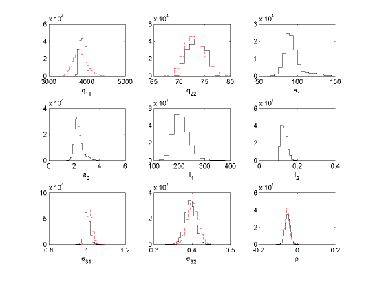
Figure 6: Marginal posterior probability densities of unknown parameters, given training data ${\bf D}$, are depicted as histograms. Histograms obtained from the run done with only within the $nested-GP$ model, shown in black, as distinguished from the results of learning given the same data, and the $nonnested-GP$ model depicted in grey (or red in the electronic copy of the thesis). Given the data used here, $s_{1}^{(test)}$ and $s_{2}^{(test)}$, are not learnt.

.

95$\%$ HPD credible regions computed on each learnt parameter given the $nonnested-GP$ model, are displayed in Table 2. Again, a similar set of results from the chains run with the $nested-GP$ models are displayed in Table 3. The results on prediction of $\boldsymbol{s}^{(test)}$ are also presented in Table 2 and Table 3.

Table 2: $95\%$ HPD credible regions on each learnt parameter, from the $nonnested-GP$ model

Parameters	using only training data	sampling from posterior predictive	sampling from joint
$q_{1}$	[3492.1,4198.1]		[3573.2,4220.8]
$q_{2}$	[68.92,76.88]		[68.37,77.33]
$\sigma^{(1)}_{11}$	[0.9837,1.0380]		[0.9797,1.0338]
$\rho$	[-0.0653,-0.0275]		[-0.0798,-0.0261]
$\sigma^{(1)}_{22}$	[0.3747,0.4234]		[0.3703,0.4237]
$s_{1}$	-	[1.8212,2.1532]	[1.8038,2.1960]
$s_{2}$	-	[0.0421,1.2052]	[0.0157,1.2172]

Table 3: $95\%$ HPD credible regions on each learnt parameter, from the $nested-GP$ model

Parameters	$t_{0}=200$	$t_{0}=100$	$t_{0}=50$
$q_{1}$	[3740.96, 3917.32]	[3710.4, 4011.66]	[3650.92, 4033.51]
$q_{2}$	[70.34, 75.70]	[70.42, 76.43]	[68.94, 76.22]
$a_{1}$	[78.67, 124.02]	[43.82, 167.35]	[48.27, 219.37]
$a_{2}$	[1.88, 3.03]	[2.12, 3.57]	[1.64, 6.16]
$d_{1}$	[155.64, 301.65]	[78.47, 521.67]	[123.42, 828.37]
$d_{2}$	[0.10, 0.15]	[0.12, 0.46]	[0.10, 0.52]
$\sigma_{31}$	[0.97, 1.02]	[0.97, 1.03]	[0.98, 1.02]
$\sigma_{32}$	[0.37, 0.41]	[0.37, 0.41]	[0.38, 0.41]
$\rho$	[-0.076, -0.031]	[-0.073, -0.03]	[-0.075, -0.032]
$s_{1}$	[1.83, 2.16]	[1.77, 2.22]	[1.76, 2.24]
$s_{2}$	[0.138, 1.15]	[0.112, 1.16]	[0.071, 1.15]

11 Model Checking

One way to check for the model and results, given the data at hand, is to generate data from the learnt model, and then compare this generated data with the observed data. Now, the model that we learn, is essentially the tensor-variate GP that is used to model the functional relationship $\boldsymbol{\xi}(\cdot)$ between the observable $\boldsymbol{V}$ and the input-space parameter $\boldsymbol{S}$. By, saying that we want to generate new data, we imply the prediction of a new value of $\boldsymbol{V}$, given the learnt model of this GP.

This prediction of new datum on $\boldsymbol{V}$, is fundamentally different from the inverse prediction of the value $\boldsymbol{s}^{(test)}$ of the input-space parameter $\boldsymbol{S}$ that we have undertaken–as discussed above–where the sought $\boldsymbol{s}^{(test)}$ is the value of $\boldsymbol{S}$ at which test data $\boldsymbol{v}^{(test)}$ on $\boldsymbol{V}$ is recorded. There is no closed-form solution to the posterior predictive of $\boldsymbol{s}^{(test)}$ given the test data and the learnt GP parameters.

In fact, at chosen values of $\boldsymbol{S}$–chosen to be the design points in the training data, for convenience–the covariance function $\boldsymbol{\Sigma}_{3}$ of this GP, (modelled as a GP with an estimated mean), is known, given the learnt values of the parameters of the kernel used to parametrise $\boldsymbol{\Sigma}_{3}$. However, in our Bayesian inference, we do not really learn a value of any parameter, but learn the marginal posterior of each unknown parameter, given the data. Thus, in order to pin the value of each element of $\boldsymbol{\Sigma}_{3}$, we identify the parameter value corresponding to a selected summary of this posterior distribution. For example, we could choose to define $\boldsymbol{\Sigma}_{3}$ at pairs of known design points $\boldsymbol{s}_{i}$, $\boldsymbol{s}_{j}$, and the modal value of $\ell_{c}$–identified from the marginal posterior of $\ell_{c}$ inferred upon, given the data. Here $i,j\in\{1,\ldots,n=216\}$. The resulting value of the $ij$-th element of $\boldsymbol{\Sigma}_{3}$ will then provide one summary, of the covariance between the $50\times 2$ stellar velocity matrix $\boldsymbol{v}_{i}$ realised at $\boldsymbol{S}=\boldsymbol{s}_{i}$, and $\boldsymbol{v}_{j}$ realised at $\boldsymbol{S}=\boldsymbol{s}_{j}$. Similarly, the learnt modal values of the parameters $\sigma_{11}^{(1)}$, $\sigma_{22}^{(1)}$ and $\rho$ define one summary of the covariance matrix $\boldsymbol{\Sigma}_{1}$ that informs on the covariance between the 2 $216\times 50$-dimensional sheets of data on each component of the 2-dimensional stellar velocity vector. Again, other summaries of the parameter values could be used as well, for example, the parameter value identified at the mean of the marginal posterior density of this parameter, as learnt given the training data, is also used.

In this model checking exercise, the unknowns are certain elements of the cuboidally-shaped data comprising the 216 number of $50\times 2$-dimensional stellar velocity matrices generated by astronomical simulation, at chosen design points $\boldsymbol{s}_{1},\ldots,\boldsymbol{s}_{216}$, i.e. the 3rd-order tensor ${\bf D}_{V}:=\{\boldsymbol{v}_{1},\vdots\boldsymbol{v}_{2},\vdots\ldots,\vdots\boldsymbol{v}_{216}\}$. In the first attempt to model checking, we generate all elements of the $q$-th such simulated stellar velocity matrix $\boldsymbol{v}_{q}$, (that is generated at the known design point $\boldsymbol{s}_{q}$), i.e. generate values of $50\times 2=100$ unknown elements of matrix $\boldsymbol{v}_{q}$. We refer to these unknown elements of $\boldsymbol{v}_{q}$ as $v_{11}^{(q)},v_{12}^{(q)},v_{21}^{(q)},\ldots,v_{50,2}^{(q)}$. The 3rd-ordered tensor without the $q$-th slice, is referred to as ${\bf D}_{V}^{(-q)}:=\{\boldsymbol{v}_{1},\vdots\boldsymbol{v}_{2},\vdots\ldots,\vdots\boldsymbol{v}_{q-1},\vdots\boldsymbol{v}_{q+1},\vdots\boldsymbol{v}_{216}\}$. The joint posterior probability density of the 100 unknowns, at the learnt modal values $q_{1}^{(mode)},q_{2}^{(mode)},\sigma_{11}^{(1,mode)},\sigma_{22}^{(1,mode)},\rho^{(mode)}$ is

$$\pi\left(v_{11}^{(q)},v_{12}^{(q)},v_{21}^{(q)},\ldots,v_{50,2}^{(q)}|{\bf D}_{V}^{(-q)}\right)\propto{\cal TN}_{2\times 50\times 216}({\hat{\boldsymbol{M}}},\boldsymbol{\Sigma}_{1}^{(mode)},{\hat{\boldsymbol{\Sigma}}}_{2},\boldsymbol{\Sigma}_{3}^{(mode)}),$$

where,
–the 3rd-ordered tensor-valued data that enters the parametric form of the 3rd-ordered tensor-normal density on the RHS, has elements of its $q$-th slice, (out of a total of 216 slices), unknown. All other elements of this $2\times 50\times 216$-dimensional tensor are known; –uniform priors are used on the unknowns; –$\boldsymbol{\Sigma}_{1}^{(mode)}$ is the learnt modal value of the $2\times 2$-dimensional covariance matrix $\boldsymbol{\Sigma}_{1}$ s.t. its $1,1$-th element is $\sigma_{11}^{(1,mode)}$, $2,2$-th element is $\sigma_{22}^{(1,mode)}$, $1,2$-th element is $\rho^{(mode)}\sqrt{\sigma_{22}^{(1,mode)}\sigma_{11}^{(1,mode)}}$, and the $2,1$-th element is equal to the $1,2$-th element (as this is a covariance matrix);
–$\boldsymbol{\Sigma}_{3}^{(mode)}$ is the learnt modal value of the $216\times 216$-dimensional covariance matrix $\boldsymbol{\Sigma}_{3}$, s.t. its $ij$-th element is $\displaystyle{\exp\left[-(\boldsymbol{s}_{i}-\boldsymbol{s}_{j})^{T}\boldsymbol{Q}^{(mode)}(\boldsymbol{s}_{i}-\boldsymbol{s}_{j})\right]}$, with the non-zero elements of the diagonal $2\times 2$-dimensional $\boldsymbol{Q}^{(mode)}$-matrix given by $q_{1}^{(mode)}$ and $q_{2}^{(mode)}$. $\boldsymbol{s}_{i}$ being the $i$-th design point, is known $\forall i,j=1,\ldots,216$.

$\begin{array}[]{c c c}{\includegraphics[width=142.26378pt]{model_checking.eps}\includegraphics[width=142.26378pt]{50x2_mode.eps}\includegraphics[width=142.26378pt]{50x2_mean.eps}}\end{array}$

Figure 7: Left: Comparison of the observed and predicted values of elements of the $q$-th $50\times 2$-dimensional stellar velocity matrix $\boldsymbol{v}_{q}$, where 216 such matrices constitute the training data ${\bf D}_{V}$ (on velocities of 50 stellar neighbours of the Sun) that is generated by astronomical simulations. The predicted or learnt values are obtained from a RW-MCMC chain undertaken with the all elements of the 3rd-order tensor ${\bf D}_{V}$ known, except for the elements of its $q$-th slice, and the learnt values of the parameters of the GP used to model the data at hand, at a chosen summary, namely the mode, of the marginal posterior density of each such learnt GP parameter. Here $q$=200. Equality of the observed and predicted values of he elements of $\boldsymbol{v}_{q}$ is indicated by the point lying on the drawn straight line with unit slope; the predicted values are found to lie close to this line. Middle: Depicts a similar comparison, as displayed in the left panel, but for 20 distinct values of $q$, namely for $q=190,191,\ldots,210$. Right: Depicts the same comparison of observed and predicted values of elements of 20 slices $\boldsymbol{v}_{190},\ldots,\boldsymbol{v}_{210}$, but this time, the employed GP parameters are the means of their respective marginals. Thus, this model-checking exercise checks for the used models and results obtained (given the data at hand) at the mean of the respective posterior.

.

To learn the 100 unknowns $v_{11}^{(q)},v_{12}^{(q)},v_{21}^{(q)},\ldots,v_{50,2}^{(q)}$, we run a RW Metropolis-Hastings chain, with the data defined as above, the known 216 number of design points, and all the learnt, modal parameter values. The joint posterior of the unknowns that defines the acceptance ratio in this chain, is given as in the last equation. The chain is run for 20,000 iterations, for $q$=200, and the mean of the last 1000 samples of $v_{ij}^{(200)}$ is recorded, where $i=1,\ldots,50$, $j=1,2$. These sample means ${\bar{v}}_{ij}^{(200)}$ then constitute the learnt value of the 100 elements of the 200-th stellar velocity matrix $\boldsymbol{v}_{200}$. We plot the pairs of learnt value ${\bar{v}}_{ij}^{(200)}$ of elements of the $\boldsymbol{v}_{200}$ matrix, against the empirically observed value of this element, $\forall i=1,\ldots,50$, $\forall j=1,2$. The plot is presented in the left panel of Figure 7. Thus, each point on this plot is a pair $({\mbox{empirically observed value of}}\>{{v}}_{ij}^{(200)},{\bar{v}}_{ij}^{(200)})$, and there are $50\times 2=100$ points in this plot. The points are found to lie around the straight line with slope 1. In other words, the values of the elements in the $q$-th (=200-th) slice of the training data that we learn using our model, are approximately equal to the empirically observed values of these elements. This is corroboration of our models and results.

We attempt a similar prediction of elements of the training data for other values of $q$, namely for $q=190,\ldots,210$. The learnt values of elements of $\boldsymbol{v}_{q}$, for each $q$, is plotted against the empirically observed elements of $\boldsymbol{v}_{q}$. We have superimposed results for all 20 values of $q$ in the same plot, resulting in the middle panel of Figure 7. Again, the values predicted for all 20 slices, are found to be close to the empirical observations, as betrayed by the points lying close to the straight line of unit slope.

Lastly, we wanted to ensure that the encouraging results from our model checking exercise is robust to changes in the posterior summary of the learnt GP parameters. Thus, we switch to using the mean of the parameter marginal posterior from the posterior mode, and carry out the same exercise of predicting elements of slices $\boldsymbol{v}_{190},\ldots,\boldsymbol{v}_{210}$. Results are displayed in the right panel of Figure 7. Again, very encouraging corroboration of our used models and results (of learning the GP parameters) is noted. Indeed, in such model checking exercises, encouraging match between the predictions and the empirical observations lends confidence in the used models and results obtained therefrom, given the data at hand–such models and results are the inputs to this exercise. However, if lack of compatibility is noted in such a model checking exercise, between empirical observations and predictions, then it implies that either the used modelling is wrong, and/or the results obtained therefrom given the data are wrong. However, the model checking exercise that we undertake, vindicates our models and results, given the data at hand.

12 Proof of Theorem 3.3 in KWDC

Theorem 12.1.

Given $\ell_{c}=g_{c,\boldsymbol{x}}(t)$, with $T\in{\cal N}\subset{\mathbb{Z}}_{\geq 0}$ and $\ell_{c}\in{\mathbb{R}}$, the map $g_{c,\boldsymbol{x}}:{\cal N}\longrightarrow{\mathbb{R}}_{\geq 0}$ is a Lipschitz-continuous map, $\forall c=1,\ldots,d$, where we know that there is a distinct value of $\ell_{c}$ generated at a given $t$, i.e. $g_{c,\boldsymbol{x}}(\cdot)$ is injective. Here ${\cal N}=\{t-1,\ldots,t-t_{0}\}$.

Proof.

Distance $d_{t_{1,2}}$ between $t_{1},t_{2}\in{\cal N}$ is $|t_{1}-t_{2}|$.

Similarly, distance $d_{g_{1,2}}$ between $g_{c,\boldsymbol{x}}(t_{1}),g_{c,\boldsymbol{x}}(t_{2})\in{\mathbb{R}}_{\geq 0}$ is $|g_{c,\boldsymbol{x}}(t_{1})-g_{c,\boldsymbol{x}}(t_{2})|$.

$${\mbox{Assume}}\quad\displaystyle{\frac{d_{g_{1,2}}}{M}}>d_{t_{1,2}},\quad M>0,\>\>M\>\>{\mbox{is finite}}\>\>\forall t_{1},t_{2}\in{\cal N}.$$

Let $\displaystyle{\frac{d_{g_{1,2}}}{M}}:=1/2$.
$\Longrightarrow|t_{1}-t_{2}|<1/2$ by our assumption,
i.e. for this choice of the LHS of the inequation assumed, the only solution for $|t_{1}-t_{2}|<1/2$ is $t_{1}=t_{2}$.
But $t_{1}=t_{2}\Longrightarrow g_{c,\boldsymbol{x}}(t_{1})=g_{c,\boldsymbol{x}}(t_{2})$ for injective $g_{c,\boldsymbol{x}}(\cdot)$, i.e. LHS of the assumed inequation is then 0.
This is a contradiction (contradicts our choice of 1/2 for the LHS).
$\therefore$ our assumption is wrong,
$\Longrightarrow$, the correct inequation is:

$${\frac{d_{g_{1,2}}}{M}}\leq d_{t_{1,2}},\quad M>0,\>\>M\>\>{\mbox{is finite}}\>\>\forall t_{1},t_{2}\in{\cal N},$$

i.e.

$${{|g_{c,\boldsymbol{x}}(t_{1})-g_{c,\boldsymbol{x}}(t_{2})|}}\leq M|t_{1}-t_{2}|,\quad M>0,\>\>M\>\>{\mbox{is finite}}\>\>\forall t_{1},t_{2}\in{\cal N}\subset{\mathbb{Z}}_{\geq 0}$$

i.e. $g_{c,\boldsymbol{x}}(\cdot)$ is Lipschitz continuous. ∎

References

- (1)
- Aston and Kirch (2012) Aston, J. A. D., and Kirch, C. (2012), “Evaluating stationarity via change-point alternatives with applications to fMRI data,” Annals of Applied Statistics, 6(4), 1906–1948.
- Barton and Fuhrmann (1993) Barton, T. A., and Fuhrmann, D. R. (1993), “Covariance structures for multidimensional data,” Multidimensional Systems and Signal Processing, 4(2), 111–123.
- Bijma et al. (2005) Bijma, F., De Munck, J. C., and Heethaar, R. M. (2005), “The spatiotemporal MEG covariance matrix modeled as a sum of Kronecker products,” NeuroImage, 27(2), 402–415.
- Chakrabarty (2004) Chakrabarty, D. (2004), “Patterns in the Outer Parts of Galactic Disks,” Monthly Notices of the Royal Astronomical Society, 352, 427.
- Chakrabarty (2007) Chakrabarty, D. (2007), “Phase space structure in the solar neighbourhood,” Astronomy & Astrophysics, 467(1), 145–162.
- Chakrabarty et al. (2015) Chakrabarty, D., Biswas, M., Bhattacharya, S. et al. (2015), “Bayesian nonparametric estimation of Milky Way parameters using matrix-variate data, in a new Gaussian Process based method,” Electronic Journal of Statistics, 9(1), 1378–1403.
- Chari, Coe, Vucic, Lockwood and Lam (2010) Chari, R., Coe, B. P., Vucic, E. A., Lockwood, W. W., and Lam, W. L. (2010), “An integrative multi-dimensional genetic and epigenetic strategy to identify aberrant genes and pathways in cancer,” BMC systems biology, 4(1), 67.
- Chari, Thu, Wilson, Lockwood, Lonergan, Coe, Malloff, Gazdar, Lam, Garnis et al. (2010) Chari, R., Thu, K. L., Wilson, I. M., Lockwood, W. W., Lonergan, K. M., Coe, B. P., Malloff, C. A., Gazdar, A. F., Lam, S., Garnis, C. et al. (2010), “Integrating the multiple dimensions of genomic and epigenomic landscapes of cancer,” Cancer and Metastasis Reviews, 29(1), 73–93.
- Clarke et al. (2008) Clarke, R., Ressom, H. W., Wang, A., Xuan, J., Liu, M. C., Gehan, E. A., and Wang, Y. (2008), “The properties of high-dimensional data spaces: implications for exploring gene and protein expression data,” Nature Reviews Cancer, 8(1), 37.
- Dryden et al. (2009) Dryden, I. L., Bai, L., Brignell, C. J., and Shen, L. (2009), “Factored principal components analysis, with applications to face recognition,” Statistics and Computing, 19(3), 229–238.
- Dunstan et al. (2013) Dunstan, P. K., Foster, S. D., Hui, F. K., and Warton, D. I. (2013), “Finite mixture of regression modeling for high-dimensional count and biomass data in ecology,” Journal of agricultural, biological, and environmental statistics, 18(3), 357–375.
- Eaton (1990) Eaton, M. L. (1990), “Chapter 8: The Wishart distribution,” in Multi-variate Statistics: A Vector Space Approach OH: Institute of Mathematical Statistics, pp. 302–333.
- Fan (2017) Fan, Y. (2017), Statistical Learning with Applications in High Dimensional Data in Health Care Analytics, PhD thesis, University of Maryland.
- Fu (2016) Fu, X. (2016), Exploring geometrical structures in high-dimensional computer vision data, PhD thesis, University of Otago.
- Gramacy (2005) Gramacy, R. (2005), Bayesian treed Gaussian process models, PhD thesis, University of California, SC.
- Hajlasz (2014) Hajlasz, P. (2014), “Geometric Analysis,” http://www.pitt.edu/ hajlasz/Notatki/Analysis4.pdf linked from http://www.pitt.edu/ hajlasz/Teaching/Math2304Spring2014/m2304Spring2014.html, .
- Heinonen et al. (2016) Heinonen, M., Mannerström, H., Rousu, J., Kaski, S., and Lähdesmäki, H. (2016), Non-Stationary Gaussian Process Regression with Hamiltonian Monte Carlo,, in Proceedings of the 19th International Conference on Artificial Intelligence and Statistics, eds. A. Gretton, and C. C. Robert, Vol. 51 of Proceedings of Machine Learning Research, PMLR, Cadiz, Spain, pp. 732–740.
- Hoff (1997) Hoff, K. (1997), “Bayesian learning in an infant industry model,” Journal of International Economics, 43(3-4), 409–436.
- Hoff et al. (2011) Hoff, P. D. et al. (2011), “Separable covariance arrays via the Tucker product, with applications to multivariate relational data,” Bayesian Analysis, 6(2), 179–196.
- Kerkheim (1994) Kerkheim, B. (1994), “Rectifiable metric spaces: local structure and regularity of the Hausdorff measure,” Proceedings of American Mathematical Society, 121, 113–124.
- Knuth (1997) Knuth, D. (1997), The Art of Computer Programming: Seminumerical Algorithms, Boston, MA, USA: Addison-Wesley Longman Publishing Co.
- Kolda and Bader (2009) Kolda, T. G., and Bader, B. W. (2009), “Tensor Decompositions and Applications,” SIAM Review, 51(3), 455–500.
- Leitao et al. (2015) Leitao, P. J., Schwieder, M., Suess, S., Catry, I., Milton, E. J., Moreira, F., Osborne, P. E., Pinto, M. J., van der Linden, S., and Hostert, P. (2015), “Mapping beta diversity from space: Sparse Generalised Dissimilarity Modelling (SGDM) for analysing high-dimensional data,” Methods in Ecology and Evolution, 6(7), 764–771.
- Manceur and Dutilleul (2013) Manceur, A. M., and Dutilleul, P. (2013), “Maximum likelihood estimation for the tensor normal distribution: Algorithm, minimum sample size, and empirical bias and dispersion,” Journal of Computational and Applied Mathematics, 239, 37 – 49.
- Mardia and Goodall (1993) Mardia, K. V., and Goodall, C. R. (1993), Spatial-temporal analysis of multivariate environmental monitoring data, Vol. 6 Elsevier New York.
- McCullagh (1987) McCullagh, P. (1987), Tensor Methods in Statistics Chapman and Hall.
- Oberg et al. (2015) Oberg, A. L., McKinney, B. A., Schaid, D. J., Pankratz, V. S., Kennedy, R. B., and Poland, G. A. (2015), “Lessons learned in the analysis of high-dimensional data in vaccinomics,” Vaccine, 33(40), 5262–5270.
- Oseledets (2011) Oseledets, I. V. (2011), “Tensor-train decomposition,” SIAM Journal on Scientific Computing, 33(5), 2295–2317.
- Paciorek and Schervish (2004) Paciorek, C., and Schervish, M. J. (2004), Nonstationary covariance functions for gaussian process regression,, in In NIPS, pp. 273–280.
- Pang et al. (2016) Pang, Y. H., Khor, E. Y., and Ooi, S. Y. (2016), Biometric Access Control with High Dimensional Facial Features,, in Australasian Conference on Information Security and Privacy, Springer, pp. 437–445.
- Qiang and Fei (2011) Qiang, Q., and Fei, Z. (2011), Generation of Facial Gesture and Expression in High-Dimensional Space,, in 2011 International Conference on Internet Technology and Applications, pp. 1–5.
- Richter et al. (2008) Richter, A., Salmi, J., and Koivunen, V. (2008), ML estimation of covariance matrix for tensor valued signals in noise,, in Acoustics, Speech and Signal Processing, 2008. ICASSP 2008. IEEE International Conference on, IEEE, pp. 2349–2352.
- Sampson and Guttorp (1992) Sampson, P., and Guttorp, P. (1992), “Nonparametric estimation of nonstationary spatial covariance structure,” Journal of the American Statistical Association, 87, 108–119.
- Sarkar (2015) Sarkar, C. (2015), Improving Predictive Modeling in High Dimensional, Heterogeneous and Sparse Health Care Data, PhD thesis, University of Minnesota.
- Schmidt and O’Hagan (2003) Schmidt, A., and O’Hagan, A. (2003), “Bayesian inference for non-stationary spatial covariance structures via spatial deformations,” Journal of the Royal Statistical Society Series B, 65, 743–758.
- Shirley (1965) Shirley, A. (1965), “The Distributed Lag Between Capital Appropriations and Expenditures,” Econometrica, 33(1), 178–196.
- Snoek et al. (2014) Snoek, J., Swersky, K., Zemel, R., and Adams, R. (2014), Input warping for bayesian optimization of non-stationary functions,, in In ICML, pp. 1674–1682.
- Theobald and Wuttke (2008) Theobald, D. L., and Wuttke, D. S. (2008), “Accurate structural correlations from maximum likelihood superpositions,” PLoS computational biology, 4(2), e43.
- Tolvanen et al. (2014) Tolvanen, V., Jylänki, P., and Vehtari, A. (2014), Expectation propagation for nonstationary heteroscedastic gaussian process regression,, in IEEE International Workshop on Machine Learning for Signal Processing (MLSP), pp. 1–6.
- Wang (2011) Wang, J. (2011), Geometric structure of high-dimensional data and dimensionality reduction Springer.
- Wang et al. (2015) Wang, W., Chen, L., and Zhang, Q. (2015), “Outsourcing high-dimensional healthcare data to cloud with personalized privacy preservation,” Computer Networks, 88, 136–148.
- Warton (2011) Warton, D. I. (2011), “Regularized Sandwich Estimators for Analysis of High-Dimensional Data Using Generalized Estimating Equations,” Biometrics, 67(1), 116–123.
- Werner et al. (2008) Werner, K., Jansson, M., and Stoica, P. (2008), “On estimation of covariance matrices with Kronecker product structure,” IEEE Transactions on Signal Processing, 56(2), 478–491.
- Wilson and Ghahramani (2011) Wilson, A., and Ghahramani, Z. (2011), Generalised Wishart Processes,, in In Proceedings of the Twenty-Seventh Conference Annual Conference on Uncertainty in Artificial Intelligence (UAI-11), Corvallis, OregonAUAI Press, pp. 736–744.
- Xu and Yan (2015) Xu, Z., and Yan, F. (2015), “Infinite Tucker Decomposition: Nonparametric Bayesian Models for Multiway Data Analysis,” arXiv:1108.6296, .
- Xu et al. (2011) Xu, Z., Yan, F. et al. (2011), “Infinite Tucker decomposition: Nonparametric Bayesian models for multiway data analysis,” arXiv preprint arXiv:1108.6296, .