Bias in OLAP Queries: Detection, Explanation, and Removal
(think twice about your group-by query)

Abstract

On line analytical processing (OLAP) is an essential element of decision-support systems. OLAP tools provide insights and understanding needed for improved decision making. However, the answers to OLAP queries can be biased and lead to perplexing and incorrect insights. In this paper, we propose HypDB, a system to detect, explain, and to resolve bias in decision-support queries. We give a simple definition of a biased query, which performs a set of independence tests on the data to detect bias. We propose a novel technique that gives explanations for bias, thus assisting an analyst in understanding what goes on. Additionally, we develop an automated method for rewriting a biased query into an unbiased query, which shows what the analyst intended to examine. In a thorough evaluation on several real datasets we show both the quality and the performance of our techniques, including the completely automatic discovery of the revolutionary insights from a famous 1973 discrimination case.

1 Introduction

On line analytical processing (OLAP) is an essential element of decision-support systems. OLAP tools enable the capability for complex calculations, analyses, and sophisticated data modeling; this aims to provide the insights and understanding needed for improved decision making. Despite the huge progress OLAP research has made in recent years, the question of whether these tools are truly suitable for decision making remains unanswered [12, 6]. The following example shows how insights obtained from OLAP queries can be perplexing and lead to poor business decisions.

Example 1.1

Suppose a company wants to choose between the business travel programs offered by two carriers, American Airlines (AA) and United Airlines (UA). The company operates at four airports: Rochester (ROC), Montrose (MTJ), McAllen Miller (MFE) and Colorado Springs (COS). It wants to choose the carrier with the lowest rate of delay at these airports. To make this decision, the company’s data analyst uses FlightData, the historical flight data from the U.S. Department of Transportation (Sec. 7.1); the analyst runs the group-by query shown in Fig. 1 to compare the performance of the carriers. Based on the analysis at the top of Fig. 1, the analyst recommends choosing AA because it has a lower average flight delay.

Surprisingly, this is a wrong decision. AA has, in fact, a higher average delay than UA at each of the four airports Fig. 1(a). This trend reversal, known as Simpson’s paradox, occurs as a result of confounding influences. The Airport has a confounding influence on the distribution of the carriers and departure delays, because its distribution differs for AA and for UA (Fig. 1 (b) and (c)): AA has many more flights from airports that have relatively few delays, like COS and MFE, while UA has more flights from ROC, which has relatively many delays. Thus, AA seems to have overall lower delay only because it has many flights from airports that in general have few delays. At the heart of the issue is an incorrect interpretation of the query; while the analyst’s goal is to compare the causal effect of the carriers on delay, the OLAP query measures only their association.

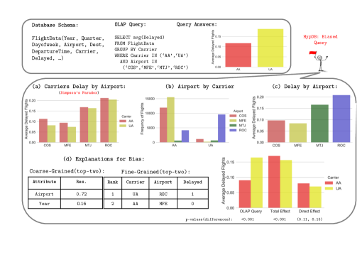
Figure 1: An OLAP query that computes the average of delayed flights for two carriers at four airports in Ex. 1.1. While AA has a lower average delay in the fours airport, UA has a lower average delay in each individual airport. HypDB explains away the anomaly, known as Simpson’s paradox, by inferring confounding attributes and query rewiring.

A principled business decision should rely on performing a hypothesis test on the causal effect of choosing between two (or more) alternatives, $T=t_{0}$ or $T=t_{1}$, on some outcome of interest, $Y$. Data analysts often reach for a simple OLAP query that computes the average of $Y$ on the two subgroups $T=t_{0}$ and $T=t_{1}$, called control and treatment subpopulations, but, as exemplified in Fig. 1, this leads to incorrect decisions. The gold standard for such causal hypothesis testing is a randomized experiment or an A/B test, called as such because the treatments are assigned to subjects randomly. In contrast, business data is observational, defined as data recorded passively and subject to selection bias. Although causal inference in observational data has been studied in statistics for decades, no causal analysis tools exist for OLAP systems. Today, most data analysts still reach for the simplest group-by queries, potentially leading to biased business decisions.

In this paper, we propose HypDB, a system to detect, explain, and resolve bias in decision-support queries. Our first contribution is a new formal definition of a biased query that enables the system to detect bias in OLAP queries by performing a set of independence tests on the data. Next, we proposed a novel technique to find explanations for the bias and to rank these explanations, thus assisting the analyst in understanding what goes on. Third, we describe a query rewriting technique to eliminate the bias from queries. To enable HypDB to perform these types of causal analysis on the data, we develop a novel algorithm to compute covariates in an efficient way. Finally, we perform extensive experiments on several real datasets and a set of synthetic datasets, demonstrating that the proposed method outperforms the state of the art causal discovery methods and that HypDB can be used interactively to detect, explain, and resolve bias at query time.

At the core of any causal analysis is the notion of a covariate, an attribute that is correlated (“covaries") with the outcome and unaffected by the treatment. For example, a $\text{Group By }T$ query is biased if there exists a set of covariates ${\mathbf{Z}}$ whose distribution differs for the different groups of $T$; Fig.1(b) shows that Airport is a covariate, as its distribution differs for AA and for UA. Thus, the OLAP query in Fig.1 is biased w.r.t. Airport. In order to draw causal conclusions from a biased query, one needs to control for covariates and thereby to eliminate other possible explanation for a causal connection indicated by the query. The statistics literature typically assumes that the covariates are given. An algorithmic approach for finding the covariates was developed by Judea Pearl [7, 43], who assumes that we are given a causal DAG over the set of attributes, where an edge represents a potential cause-effect between attributes, then gives a formal criterion, called the back-door criterion, to identify the covariates. However, in our setting the causal DAG is not given, one has to first compute the entire causal DAG from the data in order to apply Pearl’s back-door criterion. Notice that a causal DAG does not rank covariates: a variable either is, or is not a covariate. Computing the entire causal DAG is inapplicable to interactive OLAP queries for several reasons. First, computing the DAG is expensive, since causal DAG learning algorithms perform an exponential (in the number of attributes) number of iterations over the data. It is not possible to precompute the causal DAG either, because each OLAP query selects a different sub-population through the WHERE condition: this phenomenon is called population heterogeneity in statistics. Thus, the causal DAG must be computed at query time. In addition, state of the art causal DAG discovery (CDD) algorithms are not robust to sparse subpopulations, which makes them inapplicable for OLAP queries with selective WHERE conditions. We note that one should not confuse a causal DAG with an OLAP data cube: they are different things. If a precomputed OLAP cube is available, then the computation of the causal DAG can be sped up. But notice that database systems usually limit the data cube to 12 attributes, because its size is exponential in the number of attributes; in contrast, causal analysis often involves many more attributes. The FlightData dataset in our example has 101 attributes. Second, integrity constraints in databases lead to logical dependencies that totally confuse CDD algorithms: for example, FlightData satisfies the FDs “AirportWAC" $\Rightarrow$ Airport” and therefore conditioning on AirportWAC (aiport world area code), Airport becomes independent from the rest of the attributes, which breaks any causal interaction between Airport and other attributes. Typically, attributes with high entropy such as ID, FlightNum, TailNum, etc., participate in some functional dependencies. Any CDD algorithm must be adapted to handle logical dependencies before applying it to OLAP data.

In order to incorporate causal inference in OLAP, HypDB makes two key technical contributions. First, we propose a novel method for covariate discovery that does not compute the entire causal DAG, but explores only the subset relevant to the current query We empirically show that our method is competitive with state of the art CDD algorithms, yet it scales well with large and high-dimensional data, is robust to sparse subpopulations, and can handle functional dependencies on the fly. Second, we propose a powerful optimization to significantly speed up the Monte Carlo permutation-test, which is an accurate, but computationally expensive independence test needed throughout HypDB (detecting biased queries, explaining the bias, and resolving it by query rewriting). Our optimization consists of generating permutation samples without random shuffling of data, by sampling from contingency tables and conditioning groups.

Finally, a key novelty of HypDB is the ability to explain its findings, and rank the explanations. We introduce novel definitions for fine-grained and coarse-grained explanations of a query’s bias (Example 1.2). We empirically show that these explanations are crucial for decision making and reveal illuminating insights about the domain and the data collection process. For instance, HypDB reveals an inconsistency in the adult dataset [25] (Section 7).

Example 1.2

HypDB will detect that the query in Fig. 1 is biased and will explain the bias by computing a list of covariates ranked by their responsibility. Fig. 1 (d) shows that Airport has the highest responsibility, followed by Year; this provides valuable information to the data analyst for understanding the trend reversal. Finally, HypDB rewrites the original query into a query of the form Listing 2 in order to compute both the total effect and the direct effect. The total effect measures the expected changes in the delay when the carrier is set to AA and UA by a hypothetical external intervention. The direct effect measures the effect that is not mediated by other variables, such as destination and late arrival delay. Fig. 1 (d) shows that UA has a slightly better performance than AA in terms of total effect, but there is no significant difference for the direct effect.

An important application of HypDB, which we demonstrate in the empirical evaluation, is to detect algorithmic unfairness [44, 60, 57]. Here, the desire is to ensure that a machine learning algorithm does not make decisions based on protected attributes such as gender or race, for example in hiring decisions. While no generally accepted definition exists for algorithmic unfairness, it is known that any valid proof of unfairness requires evidence of causality [10]. For example, in gender discrimination, the question is whether gender has any direct effect on income or hiring [38]. We show how to use HypDB post factum to detect unfairness, by running a group-by query on the protected attribute and checking for biasness. We detect algorithmic unfairness and obtain insights that go beyond state of the art tools such as FairTest [57].

The main contributions of this paper are as follows: We provide a formal definition of a biased query based on independence tests in the data (Sec. 3.1); give a definition of responsibility and contribution, allowing us to rank attributes and their ground levels by how well they explain the bias of a query (Sec. 3.2); and describe a query rewriting procedure that eliminates bias from queries (Sec. 3.3). Then, we propose a novel algorithm for computing covariates without having to compute the complete causal DAG (Sec. 4). Next, we describe optimization techniques that speed up the independence test based on the Monte Carlo permutation-test (Sec. 5). We propose some optimizations to speed up all components of our system (Sec. 6). Finally, perform an extensive evaluation using four real datasets and a set of synthetic datasets (Sec. 7).

2 Background and Assumptions

We fix a relational schema with attributes $\mathbf{A}=\{X_{1},\ldots,X_{k}\}$ and discrete domains $Dom(X_{i}),i=1,k$. We use lower case letters to denote values in the domains, $x\in Dom(X)$, and use bolded letters for sets of attributes ${\mathbf{X}}$, or tuples $\mathbf{x}\in Dom(\mathbf{X})$ ($\stackrel{{\scriptstyle\text{def}}}{{=}}\prod_{X\in\mathbf{X}}Dom(X)$) respectively. A database instance is a set of tuples with attributes $\mathbf{A}$. We denote its cardinality by $n$.

Listing 1: An OLAP query $\mathcal{Q}$.

⬇

SELECT $T$,${\mathbf{X}}$,avg($Y_{1}$), ... ,avg($Y_{e}$)

FROM $D$

WHERE ${\mathbf{C}}$

GROUP BY $T$,${\mathbf{X}}$

We restrict the OLAP queries to group-by-average queries, as shown in Listing 1. We do not consider more complex OLAP queries (drill-down, roll-up or cube queries); we also do not consider aggregate operators other than average because they are not needed in causal analysis. To simplify the exposition we assume $T$ and $Y_{i}$ take only two values, $Dom(T)=\{t_{0},t_{1}\}$, $Dom(Y_{i})=\{0,1\}$ and denote $Dom({\mathbf{X}})=\{{\mathbf{x}}_{1}\ldots{\mathbf{x}}_{m}\}$. For each $i=1,m$ we call the condition $\Gamma_{i}\stackrel{{\scriptstyle\text{def}}}{{=}}{\mathbf{C}}\land({\mathbf{X}}={\mathbf{x}}_{i})$ a context for the query $\mathcal{Q}$. We interpret the query as follows: for each context, we want to compute the difference between $\text{avg}(Y_{i})$ for $T=t_{1}$, and for $T=t_{0}$.

We make the following key assumption, standard in statistics. The database $D$ is a uniform sample from a large population (e.g., all flights in the United States, all customers, etc.), obtained according to some unknown distribution ${\tt\mathrm{Pr}}(\mathbf{A})$. Then, the query $\mathcal{Q}$ represents a set of estimates ${\tt\mathbb{E}}[(Y_{1},\dots,Y_{e})|T=t_{j},\Gamma_{i}]$.

We assume familiarity with the notions of entropy $H(\mathbf{X})$, conditional entropy $H({\mathbf{Y}}|\mathbf{X})$, and mutual information $I(\mathbf{X};{\mathbf{Y}}|{\mathbf{Z}})$ associated to the probability distribution ${\tt\mathrm{Pr}}$; see the Appendix for a brief review. Since ${\tt\mathrm{Pr}}$ is not known, we instead estimate the entropy from the sample $D$ using the Miller-Madow estimator [32].

The Neyman-Rubin Causal Model (NRCM)

HypDB is based on the Neyman-Rubin Causal Model (NRCM) [19, 49], whose goal is to study the causal effect of a treatment variable $T\in\mathinner{\left\{t_{0},t_{1}\right\}}$ on an outcome variable $Y$. The model assumes that every object (called unit) in the population has two attributes, $Y(t_{0}),Y(t_{1})$, representing the outcome both when we don’t apply, and when we do apply the treatment to the unit. The average treatment effect (ATE) of $T$ on $Y$ is defined as:

$${\tt\textsc{ATE}}(T,Y)\stackrel{{\scriptstyle\text{def}}}{{=}}{\tt\mathbb{E}}[Y(t_{1})-Y(t_{0})]={\tt\mathbb{E}}[Y(t_{1})]-{\tt\mathbb{E}}[Y(t_{0})]$$ (1)

In general, ATE cannot be estimated from the data, because for each unit one of $Y(t_{0})$ or $Y(t_{1})$ is missing; this is called the fundamental problem of causal inference [20]. To compute the ATE, the statistics literature considers one of two assumptions. The first is the independence assumption, stating that $(Y(t_{0}),Y(t_{1}))$ is independent of $T$. Independence holds only in randomized data, where the treatment $T$ is chosen randomly, but fails in observational data, which is the focus of our work; we do not assume independence in this paper, but, for completeness, include its definition in the appendix. For observational data, we consider a second, weaker assumption [50]:

Assumption 2.1

The data contains a set of attributes ${\mathbf{Z}}\subseteq\mathbf{A}$, called covariates, satisfying the following property: forall ${\mathbf{z}}\in Dom({\mathbf{Z}})$, (1) $({Y(t_{0}),Y(t_{1})\mathrel{\text{\scalebox{1.07}{$\perp\mkern-10.0mu\perp$}}}T}|{\mathbf{Z}}={\mathbf{z}})$ (this is called Unconfoundedness), and (2) $0<\Pr(T=t_{1}|{\mathbf{Z}}={\mathbf{z}})<1$ (this is called Overlap).

Under this assumption, ATE can be computed using the following adjustment formula:

$$\small{\tt\textsc{ATE}}(T,Y)=\sum_{{\mathbf{z}}\in Dom({\mathbf{Z}})}({\tt\mathbb{E}}[Y|T=t_{1},{\mathbf{z}}]-{\tt\mathbb{E}}[Y|T=t_{0},{\mathbf{z}}])\ \Pr({\mathbf{z}})$$ (2)

Example 2.2

Referring to our example 1.1, we assume that each flight has two delay attributes, $Y(\text{AA})$ and $Y(\text{UA})$, representing the delay if the flight were serviced by AA, or by UA respectively. Of course, each flight was operated by either AA or UA, hence $Y$ is either $Y(\text{AA})$ or $Y(\text{UA})$ in the database; the other one is missing, and we can only imagine it in an alternative, counterfactual world. The independence assumption would require a controlled experiment, where we assign randomly each flight to either AA or UA, presumably right before the flight happens, clearly an impossible task. Instead, under the Unconfoundedness assumption we have to find sufficient covariates, such that, after conditioning, both delay variables are independent of which airline operates the flight. We note that “independence” here is quite subtle. Clearly the delay $Y$ is dependent of the airline, because it depends on whether the flight is operated by AA or UA. What the assumption states is that, after conditioning, the delay of the flight if it were operated by AA (i.e. $Y(\text{AA})$) is independent of whether the flight is actually operated by AA or UA, and similarly for $Y(\text{UA})$.

To summarize, in order to compute ATE, one has to find the covariates ${\mathbf{Z}}$. The overlap condition is required to ensure that (2) is well defined, but in practice overlap often fails on the data $D$. The common approach is to select covariates ${\mathbf{Z}}$ that satisfy only Unconfoundedness, then estimate (2) on the subset of the data where overlap holds, see Sec. 3.3. Thus, our goal is to find covariates satisfying Unconfoundedness.

Causal DAGs. A causal DAG $G$ is graph whose nodes are the set of attributes $V(G)=\mathbf{A}$ and whose edges $E(G)$ capture all potential causes between the variables [38, 39, 7]. We denote ${\mathbf{PA}}_{X}$ the set of parents of $X$. If there exists a directed path from $X$ to $Y$ then we say that $X$ is an ancestor or a cause of $Y$, and say that $Y$ is a descendant or an effect of $X$. A probability distribution $\Pr({\mathbf{A}})$ is called causal, or DAG-isomorphic, if there exists a DAG $G$ with nodes ${\mathbf{A}}$ that captures precisely its independence relations[42, 39, 56]: the formal definition is in the appendix, and is not critical for the rest of the paper. Throughout this paper we assume $\Pr$ is DAG-isomorphic.

Covariate Selection. Fix some database $D$, representing a sample of some unknown distribution $\Pr$, and suppose we want to compute the causal effect of an attribute $T$ on some other attribute $Y$. Suppose that we computed somehow a causal DAG $G$ isomorphic to $\Pr({\mathbf{A}})$. Pearl [37] showed that the parents of $T$ are always a sufficient set of covariates, more precisely:

Proposition 2.3

[39, Th. 3.2.5] Fix two attributes $T$ and $Y$. Then the set of parents, ${\mathbf{Z}}\stackrel{{\scriptstyle\text{def}}}{{=}}{\mathbf{PA}}_{T}$ satisfies the Unconfoundedness property.

In HypDB we always choose ${\mathbf{PA}}_{T}$ as covariates, and estimate ATE using Eq. (2) on the subset of the data where overlap holds; we give the details in Sec. 3.3.

Learning the Parents from the Data. The problem is that we do not have the causal dag $G$, we only have the data $D$. Learning the causal DAG from the data is considered to be a challenging task, and there are two general approaches. The score-based approach [18] uses a heuristic score function on DAGs and a greedy search. The constraint-based approach [47, 40] builds the graph by repeatedly checking for independence relations in the data. Both approaches are expensive, as we explain in Sec. 4, and unsuitable for interactive settings. Furthermore, in our application the causal DAG must be computed at query time, because it depends on the WHERE condition of the query. Instead, to improve the efficiency of HypDB, we compute only ${\mathbf{PA}}_{T}$, by using the Markov Boundary.

Definition 2.4

[42] Fix a probability distribution $\Pr({\mathbf{A}})$ and a variable $X\in{\mathbf{A}}$. A set of variables ${\mathbf{B}}\subseteq{\mathbf{A}}-\mathinner{\left\{X\right\}}$ is called a Markov Blanket of $X$ if $(X\mbox{$\perp\!\!\!\perp$}{\mathbf{A}}-{\mathbf{B}}-\mathinner{\left\{X\right\}}|{\mathbf{B}})$; it is called a Markov Boundary if it is minimal w.r.t. set inclusion.

Next, we relate the Markov boundary of $T$ with ${\mathbf{PA}}_{T}$:

Proposition 2.5

[34, The. 2.14] Suppose $P(\mathbf{A})$ is DAG-isomorphic with $G$. Then for each variable $X$, the set of all parents of $X$, children of $X$, and parents of children of $X$ is the unique Markov boundary of $X$, denoted ${\mathbf{B}}(X)$.

Thus, ${\mathbf{PA}}_{T}\subseteq{\mathbf{B}}(T)$. Several algorithms exists in the literature for computing the blanket, ${\mathbf{B}}(T)$, for example the Grow-Shrink [28]. In Sec. 4 we describe a novel technique that, once ${\mathbf{B}}(T)$ is computed, extracts the parents ${\mathbf{PA}}_{T}$.

Total and Direct Effects. ATE measures the total effect of $T$ on $Y$, aggregating over all directed paths from $T$ to $Y$. In some cases we want to investigate the natural direct effect, NDE [38], which measures the effect only through a single edge from $T$ to $Y$. Its definition is rather technical and deferred to the appendix. For the rest of the paper it suffices to note that it can be computed using the following formula [38], ${\tt\textsc{NDE}}(T,Y)=$

$$\sum_{\parbox{14.22636pt}{\mbox{\scriptsize$({\mathbf{z}},{\mathbf{m}})\in Dom({\mathbf{Z}},{\mathbf{M}})$}}}({\tt\mathbb{E}}[Y|T=t_{0},{\mathbf{m}}]-{\tt\mathbb{E}}[Y|T=t_{1},{\mathbf{m}}])\Pr({\mathbf{m}}|T=t_{1},{\mathbf{z}})\Pr({\mathbf{z}})\$$ (3)

where the covariates are ${\mathbf{Z}}\stackrel{{\scriptstyle\text{def}}}{{=}}{\mathbf{PA}}_{T}$, and ${\mathbf{M}}\stackrel{{\scriptstyle\text{def}}}{{=}}{\mathbf{PA}}_{Y}-\{T\}$ is called the set of mediators. HypDB computes both total and direct effect.

3 Biased OLAP Queries

We introduce now the three main components of HypDB: the definition of bias in queries, a novel approach to explain bias, and a technique to eliminate bias. Throughout this section, we will assume that the user issues a query $\mathcal{Q}$ (Listing 1), with intent to study the causal effect (total or direct) from $T$ to $Y_{j}$, for each outcome variable $Y_{j}$, and for each context $\Gamma_{i}$. We assume that we are given the set of covariates ${\mathbf{Z}}$ (for the total effect) or covariates ${\mathbf{Z}}$ and mediators ${\mathbf{M}}$ (for the direct effect); next section explains how to compute them. We assume that all query variables other than treatment and outcome are included in ${\mathbf{Z}}$, or ${\mathbf{Z}}\cup{\mathbf{M}}$ respectively.

3.1 Detecting Bias

Let ${\mathbf{V}}$ denote ${\mathbf{Z}}$ for total effect, or ${\mathbf{Z}}\cup{\mathbf{M}}$ for direct effect.

Definition 3.1

We say the query $\mathcal{Q}$ is balanced w.r.t. a set of variables ${\mathbf{V}}$ in a context $\Gamma_{i}$ if the marginal distributions $\Pr({\mathbf{V}}|T=t_{0},\Gamma_{i})$ and $\Pr({\mathbf{V}}|T=t_{1},\Gamma_{i})$ are the same.

Equivalently, $\mathcal{Q}$ is balanced w.r.t. ${\mathbf{V}}$ in the context $\Gamma_{i}$ iff $(T\mbox{$\perp\!\!\!\perp$}{\mathbf{V}}|\Gamma_{i})$. We prove (in the appendix):

Proposition 3.2

Fix a context $\Gamma_{i}$ of the query $\mathcal{Q}$, and let $\Delta_{i}$ denote the difference between $\text{avg}({\mathbf{Y}})$ for $T=t_{1}$ and for $T=t_{0}$ ($\Delta_{i}$ estimates ${\tt\mathbb{E}}[{\mathbf{Y}}|T=t_{1},\Gamma_{i}]-{\tt\mathbb{E}}[{\mathbf{Y}}|T=t_{0}|\Gamma_{i}]$). Then:

• if $\mathcal{Q}$ is balanced w.r.t. the covariates ${\mathbf{Z}}$ in the context $\Gamma_{i}$, then $\Delta_{i}$ is an unbiased estimate of the ATE (Eq. (1)). In this case, with some abuse, we say that $\mathcal{Q}$ is unbiased for estimating total effect.

• if $\mathcal{Q}$ is balanced w.r.t. the covariates and mediators ${\mathbf{Z}}\cup{\mathbf{M}}$ in the context $\Gamma_{i}$, then $\Delta_{i}$ is an unbiased estimate of NDE (Eq. (7)); we say that $\mathcal{Q}$ is unbiased for estimating direct effect.

In other words, if the query is unbiased w.r.t. the covariates ${\mathbf{Z}}$ (and mediators ${\mathbf{M}}$) then the user’s query is an unbiased estimator, as she expected. In that case the groups are comparable in every relevant respect, i.e., the distribution of potential covariates such as age, proportion of male/female, qualifications, motivation, experience, abilities, etc., are similar in all groups. The population defined by the query’s context behaves like a randomization experiment.

During typical data exploration, however, queries are biased. In Ex. 1.1, the distribution of the covariate Airport differs across the two groups formed by Carrier (Fig. 1(b)). This makes the groups incomparable and the query biased in favor of AA, because AA has many more flights from airports that have few delays, like COS and MFE, while UA has more flights from ROC, which has many delays (Fig. 1 (b) and (c)).

To detect whether a query is unbiased w.r.t. ${\mathbf{V}}$, we need to check if $(T\mbox{$\perp\!\!\!\perp$}{\mathbf{V}}|\Gamma_{i})$, or equivalently if $I(T;{\mathbf{V}}|\Gamma_{i})=0$, where $I$ is the conditional mutual information. Recall that $I$ is defined by the unknown probability distribution $\Pr$ and cannot be computed exactly. Instead, we have the database $D$, which is a sample of the entire population, we estimate $\hat{I}$, then check dependence by rejecting the null hypothesis $I(T;{\mathbf{V}}|\Gamma_{i})=0$ if the $p$-value is small enough. (Even if $D$ consists of the entire population, the exact equality $I(T;{\mathbf{V}}|\Gamma_{i})=0$ is unlikely to hold for the uniform distribution $\Pr$ over $D$.) We discuss this in detail in Sec. 5. For an illustration, in Ex. 1.1, $\hat{I}(\text{Carrier};\text{Aiport}|\Gamma)=0.25\neq 0$ with p-value$<0.001$, where $\Gamma$ is the context of the four airports. Thus, the query is biased.

3.2 Explaining Bias

In this section, we propose novel techniques to explain the bias in the query $\mathcal{Q}$. We provide two kinds of explanations: coarse grained explanations consist of a list of attributes $Z\in{\mathbf{Z}}$ (or ${\mathbf{Z}}\cup{\mathbf{M}}$), ranked by their responsibility to the bias, and fine grained explanations, consisting of categories (data values) of each attribute $Z$, ranked by their contribution to bias.

Coarse-grained. Our coarse-grained explanation consists of ranking the variables ${\mathbf{V}}$ (which is either ${\mathbf{Z}}$ or ${\mathbf{Z}}\cup{\mathbf{M}}$), in terms of their responsibilities for the bias, which we measure as follows:

Definition 3.3

(Degree of Responsibility): We define the degree of responsibility of a variable $Z\in{\mathbf{V}}$ in the context $\Gamma_{i}$ as

$$\rho_{Z}=\frac{I(T;{\mathbf{V}}|\Gamma_{i})-I(T;{\mathbf{V}}|Z,\Gamma_{i})}{\sum_{V\in{\mathbf{V}}}I(T;{\mathbf{V}}|\Gamma_{i})-I(T;{\mathbf{V}}|V,\Gamma_{i})}$$ (4)

When $Z\in{\mathbf{V}}$, the quantity $I(T;{\mathbf{V}}|\Gamma_{i})-I(T;{\mathbf{V}}|Z,\Gamma_{i})$ is always $\geq 0$. Therefore $\rho_{Z}$ is simply the normalized value of some positive quantities, and thus $0\leq\rho_{Z}\leq 1$. The larger $\rho_{Z}$, the more responsible $V$ is for bias. The intuition is that there is no bias iff $I(T;{\mathbf{V}}|\Gamma_{i})=0$, thus the degree of responsibility measures the contribution of a single variable to the inequality $I(T;{\mathbf{V}}|\Gamma_{i})>0$.

HypDB generates coarse-grained explanations for a biased query, by ranking covariates and mediators in terms of their responsibilities. In Ex. 1.1, the covariates consists of attributes such as Airport, Day, Month, Quarter, Year. Among them Airport has the highest responsibility, followed by Year (Fig. 1 (d)). See Sec. 7 for more examples.

Fine-Grained. A fine-grained explanation for a variable $Z\in{\mathbf{V}}$ is a triple $(t,y,z)$, where $t\in Dom(T)$, $y\in Dom(Y)$, $z\in Dom(Z)$, that highly contributes to both $I(T;Z)$ and $I(Y;Z)$. These triples explain the confounding (or mediating) relationships between the ground levels. We measure these contributions as follows:

Definition 3.4

(Degree of contribution): Given two variables $X,Y\in\mathbf{A}$ with $I(X;Y)>0$ and a pair $(x,y)\in Dom(XY)$, we define the degree of contribution of $(x,y)$ to $I(X;Y)$ as:

$$\kappa_{(x,y)}={{\tt\mathrm{Pr}}(x,y)\log(\frac{{\tt\mathrm{Pr}}(x,y)}{{\tt\mathrm{Pr}}(x){\tt\mathrm{Pr}}(y)})}$$ (5)

Mutual information satisfies $I(X;Y)=\sum_{(x,y)\in Dom({\mathbf{X}},{\mathbf{Y}})}\kappa_{(x,y)}$. Thus, a pair $(x,y)$ can either make a positive ($\kappa_{(x,y)}>0$), negative ($\kappa_{(x,y)}<0$), or no contribution ($\kappa_{(x,y)}=0$) to $I(X;Y)$.

To compute the contribution of the triples $(t,y,z)$ to both $I(T;Z|\Gamma_{i})$ and $I(Y;Z|\Gamma_{i})$ and generate explanations, HypDB proceeds as follows. It first ranks all triples $(t,y,z)\in\Pi_{TYZ}(\sigma_{\Gamma_{i}}(D))$, based on their contributions to $\hat{I}(T;Z)$, then it ranks them again based on their contribution to $\hat{I}(Y;Z)$, then aggregates the two rankings using Borda’s methods [26]; we give the details in the algorithm FGE  in Alg. 3 in the appendix. HypDB returns the top $k$ highest ranked triples to the user. For example, Fig. 1(d) shows the triple (Airport=ROC, Carrier=UA, Delayed=1) as the top explanation for the $Z=\text{Airport}$ covariate; notice that this captures exactly the intuition described in Ex. 1.1 for the trend reversal.

Listing 2: Refined OLAP query ${{\mathcal{Q}_{rw}}}$.

⬇

WITH Blocks

AS(

SELECT $T$,${\mathbf{X}}$,${\mathbf{Z}}$,avg($Y_{1}$) AS Avg1,...,avg($Y_{e}$) AS Avge

FROM $D$

WHERE ${\mathbf{C}}$

GROUP BY $T$,${\mathbf{Z}}$,${\mathbf{X}}$),

Weights

AS(

SELECT${\mathbf{X}}$,${\mathbf{Z}},$count(*)/$n$ AS W

FROM $D$

WHERE ${\mathbf{C}}$

GROUP BY ${\mathbf{Z}}$,${\mathbf{X}}$

HAVING count(DISTINCT $T$)=2)

SELECT $T$,${\mathbf{X}}$,sum(Avg1 * W),...,sum(Avge * W)

FROM Blocks,Weights

WHERE Blocks.${\mathbf{Z}}$ = Weights.${\mathbf{Z}}$ AND

Blocks.${\mathbf{X}}$ = Weights.${\mathbf{X}}$

GROUP BY $T$,${\mathbf{X}}$

3.3 Resolving Bias

Finally, HypDB can automatically rewrite the query to remove the bias, by conditioning on the covariates ${\mathbf{Z}}$ (recall that we assumed in this section the covariates to be known). Listing 2 shows the general form of the rewritten query ${{\mathcal{Q}_{rw}}}$ for computing the total effect of $\mathcal{Q}$ (Listing 1). The query ${{\mathcal{Q}_{rw}}}$ essentially implements the adjustment formula Eq. (2); it partitions the data into blocks that are homogeneous on ${\mathbf{Z}}$. It then computes the average of each $Y\in{\mathbf{Y}}$ Group by $T,{\mathbf{X}}$, in each block. Finally, it aggregates the block’s averages by taking their weighted average, where the weights are probabilities of the blocks. In order to enforce the overlap requirement (Assumption 2.1) we discard all blocks that do not have at least one tuple with $T=t_{1}$ and one tuple with $T=t_{0}$; this pruning technique is used in causal inference in statistics, and is known as exact matching [21]. We express exact matching in SQL using the condition $\texttt{count(DISTINCT T)}=2$, ensuring that for every group $t_{0},{\mathbf{x}},\texttt{avg}_{1},\ldots$ in the query answer, there exits a matching group $t_{1},{\mathbf{x}},\texttt{avg}_{1}^{\prime},\ldots$, and vice versa. Note that probabilities need to be computed wrt. the size of renaming data after pruning. The API of HypDB finds these matching groups, and computes the differences $\texttt{avg}_{i}^{\prime}-\texttt{avg}_{i}$, for $i=1,e$; this represents precisely the ATE for that context, Eq. (1). The rewritten query associated to Ex. 1.1 is shown in Listing 3, in the appendix.

HypDB performs a similar rewriting for computing the direct effects of $T$ on covariates ${\mathbf{Y}}$ and mediators ${\mathbf{M}}$, by implementing the mediator formula (Eq. 3).

4 Automatic Covariates Discovery

In this section we present our algorithm for automatic covariates discovery from the data. More precisely, given a treatment variable $T$, our algorithm computes its parents in the causal DAG, ${\mathbf{PA}}_{T}$, and sets ${\mathbf{Z}}={\mathbf{PA}}_{T}$ (Prop. 2.3); importantly, our algorithm discovers ${\mathbf{PA}}_{T}$ directly from the data, without computing the entire DAG.

In this section we assume to have an oracle for testing conditional independence $(U\mbox{$\perp\!\!\!\perp$}V|W)$ in the data; we describe this algorithm in the next section. Using repeated independence tests, we can compute the Markov Boundary of $T$, ${\bf MB}(T)$, e.g. using the Grow-Shrink algorithm [28]. While ${\mathbf{PA}}_{T}\subseteq{\bf MB}(T)$, identifying the parents is difficult because it is sometimes impossible to determine the direction of the edges. For example, consider a dataset with three attributes $T,W,Z$ and a single independence relation, $(Z\mbox{$\perp\!\!\!\perp$}W|T)$. This is consistent with three causal DAGs: $Z\rightarrow T\rightarrow W$, or $Z\leftarrow T\leftarrow W$, or $Z\leftarrow T\rightarrow W$, and ${\mathbf{PA}}_{T}$ is either $Z$, or $W$, or $\emptyset$. A Markov equivalence class [56] is a set of causal DAGs that encode the same independence assumptions, and it is well known that one cannot distinguish between them using only the data. For that reason, in HypDB we make the following assumption: for every $U\in{\mathbf{PA}}_{T}$ there exists $V\in{\mathbf{PA}}_{T}$ such that $U,V$ are not neighbors. Intuitively, the assumption says that ${\mathbf{PA}}_{T}$ is big enough: if ${\mathbf{PA}}_{T}=\emptyset$, then there is no need to choose any covariates (i.e. ${\mathbf{Z}}=\emptyset$), so the only setting where our assumption fails is when $T$ has a single parent, or all its parents are neighbors. In the former case, HypDB sets ${\mathbf{Z}}={\bf MB}(T)-\{Y\}$. In the latter case, parents of $T$ can not be learned from data. However, one can compute a set of potential parents of $T$ and use them to establish a bound on causal effect. For example, in the causal DAG $G$ consists of edges $(U,V)$, $(V,T)$, $(U,T)$, $(T,Y)$ and $(U,Y)$, parents of $T$ are neighbors and can not be learned from data. However, to compute the effect of $T$ on $Y$, one can learn ${\bf MB}(T)=\{U,V,Y\}$ from data, and then set ${\mathbf{Z}}=\{U,V\}$, ${\mathbf{Z}}=\{U\}$, ${\mathbf{Z}}=\{V\}$ and ${\mathbf{Z}}=\emptyset$, i.e., all subsets of ${\bf MB}(T)-\{Y\}$, to infer a bound on the effect. We leave this extension for future work. Given our assumption, we prove:

Proposition 4.1

Let $\Pr$ be DAG-isomorphic with $G$, $T\in V(G)$, and $Z\in{\bf MB}(T)$. Then $Z\in{\mathbf{PA}}_{T}$ iff both conditions hold:

• There exists $W\in{\bf MB}(T)-\mathinner{\left\{Z\right\}}$ and ${\mathbf{S}}\subseteq{\bf MB}(Z)-\mathinner{\left\{W,T\right\}}$ such that $(Z\mbox{$\perp\!\!\!\perp$}W|{\mathbf{S}})\land(Z\mbox{$\not\!\perp\!\!\!\perp$}W|{\mathbf{S}}\cup\{T\})$

• Forall ${\mathbf{S^{\prime}}}\subset{\bf MB}(T)-\{Z\}$, $(Z\mbox{$\not\!\perp\!\!\!\perp$}T|{\mathbf{S^{\prime}}})$

The intuition behind this proposition is that a necessary condition for $Z,W\in{\bf MB}(T)$ to be the parents of $T$ is that $T$ be a collider in a path between them. In causal DAG terms, a common descendant of two nodes is called a collider node, because two arrowheads collide at this node (see Appendix 10.1 for a formal definition and example). If $Z$ and $W$ are not neighbors this can be detected from data by performing a series of independence tests to check for the condition (a). For instance, in the causal DAG in Fig. 2 ($Z\mbox{$\perp\!\!\!\perp$}W$) but ($Z\not\mbox{$\perp\!\!\!\perp$}W|T$), thus (a) holds for ${\mathbf{S}}=\emptyset$. However, (a) is only necessary but not sufficient. In Fig. 2, $D\mbox{$\perp\!\!\!\perp$}W$ and $D\not\mbox{$\perp\!\!\!\perp$}W|T$, but $D$ is not a parent of $T$. This would happen if $T$ were a collider in a path between one of its parents, e.g., $W$, and a parent of its children, e.g., $D$, that are (conditionally) independent. Condition (b) excludes such cases by removing all those that are not neighbor with $T$. Furthermore, to check (a) and (b), it is sufficient to restrict the search to subsets of the relevant Markov boundaries.

The CD algorithm, shown in Alg 1, implements this idea in two phases. In phase I, it collects in ${\mathbf{C}}$ the set of all pairs of variables that satisfy (a). Note that (a) is a symmetric property. At the end of this step ${\mathbf{C}}$ consists of all parents of $T$ and possibly parents of its children. In phase II, those variables in ${\mathbf{C}}$ that violate (b) will be discarded, in a single iteration over the subsets of ${\bf MB}(T)$. At the end of this step ${\mathbf{C}}$ consists of all and only parents of $T$. While the CD algorithm uses principles similar to those used by the constrained-based CDD methods (Sec 2), its local two-phase search strategy is novel and optimized for the discovery of parents. In contrast to other constraint-based algorithms that learn the structure of a DAG by first identifying all direct neighbors of the nodes, the CD algorithm only checks whether a node is a neighbor of $T$ if it satisfies (a). In Sec. 7, we empirically show that our algorithm is more robust and efficient for covariates discovery than other CDD methods. The worst case complexity of the algorithm is exponential in the size of the largest Markov boundary it explores, which is typically much smaller than the number of attributes. In Ex. 1.1, Markov Boundary of Carrier consists of only 5 out of 101 attributes in FlightData. Thus, our approach is effective for causal DAGs with bounded fan-ins. In Sec. 7, the largest Markov boundary computed in the experiments consists of 8 attributes.

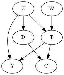
Figure 2: Example of a causal DAG.

Input: A dataset $D$, and a treatment $T\in\mathbf{A}$

Output: A set of covariates ${\mathbf{Z}}$

1 ${\mathbf{C}}\leftarrow\emptyset$

2 $\triangleright$ Phase I

3 for $Z\in{\bf MB}(T)$ s.t. $Z\not\in{\mathbf{C}}$ do

4       for ${\mathbf{S}}\subseteq{\bf MB}(Z)-\{T\}$ do

5             if  $\exists\ W\in{\bf MB}(T)$ s.t. $(Z\mbox{$\perp\!\!\!\perp$}W\ |{\mathbf{S}})\land(Z\mbox{$\not\!\perp\!\!\!\perp$}W\ |\ {\mathbf{S}}\cup\{T\})$ then

6                   ${\mathbf{C}}\leftarrow{\mathbf{C}}\cup\{Z,W\}$

7                   Break

8                  

9            

10      

11 $\triangleright$ Phase II

12 for $C\in{\mathbf{C}}$ do

13       if  $\exists\ {\mathbf{S}}\subseteq{\bf MB}(T)-\{C\}$ s.t. $(T\mbox{$\perp\!\!\!\perp$}C\ |{\mathbf{S}})$ then

14             ${\mathbf{C}}\leftarrow{\mathbf{C}}-\{C\}$

15            

16      

17${\mathbf{Z}}\leftarrow{\mathbf{C}}$

return ${\mathbf{Z}}$

Algorithm 1 Covariate Detection (CD)

HypDB applies the CD algorithm to the subpopulation specifies by the WHERE clause of $\mathcal{Q}$, assuming homogeneity in the contexts formed by the grouping attributes. Note that for computing the direct effect of $T$ on each outcome $Y_{j}$, the parents of ${\mathbf{PA}}_{Y_{j}}$ must be also learned from data (Sec. 2), using the CD algorithm.

Dropping logical dependencies. As discuss in the introduction, logical dependencies such as keys or functional dependencies can completely confuse inference algorithms; for example, if the FD $X\Rightarrow T$ holds then ${\bf MB}(T)=\mathinner{\left\{X\right\}}$, thus totally isolating $T$ from the rest of the DAG. HypDB performs the following steps. Before computing the Markov boundary of a variable $T$ , it discards all attributes $X\in\mathbf{A}$ such that $H(T|X)=\epsilon$ and $H(X|T)=\epsilon$ for $\epsilon\approx 0$. These tests correspond to approximate FDs, for example AirportWAC $\Rightarrow$ Airport. In addition, it drops attributes such as ID, FlightNum, TailNum, etc., that have high entropy and either individually or in combination form key constraints. Attributes with high entropy are either uninteresting or must be further refined into finer categories. One possibility is to choose a cut point $\alpha$ and discard attributes $X\in\mathbf{A}$ with $H(X)>\alpha$. Instead, HypDB draws a set of small random samples from data, computes the entropy of all attributes in each sample, and uses an independence test to check whether entropies of the attributes in different samples depends on the sample sizes. The intuition is that entropy is a property of the underlying generative distribution Pr, not the size of a sample. For attributes such as ID, sample size functionally determines the entropy. Attributes with high entropy are either uninteresting or must be further refined into finer categories.

Input: A dataset $D$, two variables $T,Y\in\mathbf{A}$ and a set ${\mathbf{Z}}\subset\mathbf{A}$, number of permutation samples $m$

Output: Significant level of $\hat{I}(T,Y|{\mathbf{Z}})$

1

2$s_{0}\leftarrow\hat{I}(X,Y|{\mathbf{Z}})$

3 for ${\mathbf{z}}\in\Pi_{{\mathbf{Z}}}(D)$ do

4       for $i\in\{1\ldots m\}$ do

5             $CT_{i}\ \leftarrow{\mathbf{RandT}}(\mathcal{C}^{X}_{\sigma_{{\mathbf{Z}}={\mathbf{z}}}(D)}$, $\mathcal{C}^{Y}_{\sigma_{{\mathbf{Z}}={\mathbf{z}}}(D)})$

6             $S[{\mathbf{z}},i]\leftarrow\hat{I}_{\mathcal{C}_{i}}(X,Y)$

7            

8      

9$\hat{\alpha}\leftarrow 0$

10 for $i\in\{1,\dots,m\}$ do

11       $s_{i}\leftarrow 0$

12       for ${\mathbf{z}}\in\Pi_{{\mathbf{Z}}}(D))$ do

13             $s_{i}=+S[{\mathbf{z}},i]\times{\tt\mathrm{Pr}}({\mathbf{Z}}={\mathbf{z}})$

14      if $s_{i}>s_{0}$  then

15            $\hat{\alpha}=+\frac{1}{m}$.

16      

17$\textnormal{{return}}\ \hat{\alpha}\mathbin{\leavevmode\hbox to6.46pt{\vbox to5.98pt{\text{[drawing]}}}}1.96\ \sqrt{\frac{\hat{\alpha}\ (1-\hat{\alpha})}{m}}$

Algorithm 2 Mutual Information Test (MIT)

5 Efficient Independence Test

In this section we describe our algorithm for checking conditional independence in the data. The problem of determining significance of dependency can be formulated as a chi-squared test [15], G-test [29] or as exact tests such as the permutation test [14]. The permutation test applies to the most general settings, and is non-parametric, but it is also computationally very expensive. In this section we propose new optimization methods that significantly speedup the permutation test. We start with the brief review.

Monte-Carlo permutation test. $(T\mbox{$\perp\!\!\!\perp$}Y|{\mathbf{Z}})$ holds iff $I(T;Y|{\mathbf{Z}})=0$, but in practice we can only estimate $\hat{I}(T;Y|{\mathbf{Z}})=v$. The aim of the permutation test is to compute the p-value of a hypothesis test: under the null-hypothesis $I(T;Y|{\mathbf{Z}})=0$, compute the probability that the estimate $\hat{I}(T;Y|{\mathbf{Z}})$ is $\geq v$. The distribution of the estimate $\hat{I}$ under the null-hypothesis can be computed using the following Monte-Carlo simulation: permute the values of the attribute $T$ in the data within each group of the attributes ${\mathbf{Z}}$, re-compute $\hat{I}$, and return the probability of $\hat{I}\geq v$. In other words, for each ${\mathbf{z}}\in\Pi_{{\mathbf{Z}}}(D)$, we compute $\sigma_{{\mathbf{Z}}={\mathbf{z}}}(D)$, randomly permute the values in the $T$ column (the permutation destroys any conditional dependence that may have existed between $T$ and $Y$), then recompute $\hat{I}$, and set the p-value $\alpha$ to the fraction of the $m$ trials where $\hat{I}\geq v$.

The Monte Carlo simulation needs to be performed a sufficiently large number of times, $m$, and each simulation requires permuting the entire database. This is infeasible even for small datasets. Our optimization uses contingency tables instead.

Permutation test using contingency tables. A contingency table is a tabular summarization of categorical data. A k-way contingency table over $\mathbf{A}$ is a $k$-dimensional array of non-negative integers $\mathcal{C}^{\mathbf{A}}_{D}=\{n({\mathbf{i}})\}_{{\mathbf{i}}\in{\mathbf{D}}om(\mathbf{A})}$, where $n({\mathbf{i}})=\sum_{\mathbf{a}\in D}1_{\mathbf{a}={\mathbf{i}}}$. For any ${\mathbf{X}}\subseteq\mathbf{A}$, marginal frequencies can be obtained by summation over ${\mathbf{X}}$. For instance, the following table shows a $2\times 2$ contingency table over $T$ and $Y$ together with all marginal probabilities.

	$Y=1$	$Y=0$
$T=1$	$n_{11}$	$n_{10}$	$n_{1\_}$
$T=0$	$n_{01}$	$n_{00}$	$n_{0\_}$
	$n_{\_1}$	$n_{\_0}$	$n_{\_\_}$

Randomly shuffling data only changes the entries of a contingency table, leaving all marginal frequencies unchanged (or equivalently, shuffling data does not change the marginal entropies). Thus, instead of drawing random permutations by shuffling data, one can draw them directly from the distribution of all contingency tables with fixed marginals. An efficient way to do this sampling is to use Patefield’s algorithm[36]. This algorithm accepts marginals of an $i\times j$ contingency table and generates $m$ random contingency tables with the given marginals, where the probability of obtaining a table is the same as the probability of drawing it by randomly shuffling.

Based on this observation, we develop MIT, a non-parametric test for significance of conditional mutual information, shown in Alg. 2. To test the significance of $\hat{I}(T;Y|{\mathbf{Z}})$, for each ${\mathbf{z}}\in\Pi_{{\mathbf{Z}}}(D)$, MIT takes $m$ samples from the distribution of the contingency table with fixed marginals $\mathcal{C}^{X}_{\sigma_{{\mathbf{Z}}={\mathbf{z}}}(D)}$ and $\mathcal{C}^{Y}_{\sigma_{{\mathbf{Z}}={\mathbf{z}}}(D)}$ using Patefield’s algorithm. Then, it computes $\hat{I}_{C_{i}}(T;Y)$, the mutual information between $T$ and $Y$ in the distribution defined by a random contingency table $C_{i}$. These results are aggregated using the equation $I(T;Y|{\mathbf{Z}})={\tt\mathbb{E}}_{{\mathbf{z}}}[I(T;Y)|{\mathbf{Z}}={\mathbf{z}}]$ to compute the test statistic in each permutation sample. Finally, MIT computes a 95% binomial proportion confidence interval around the observed p-value.

As opposed to the complexity of shuffling data, which is proportional to the size of the data, the complexity of Patefield’s algorithm is proportional to the dimensions of $T$ and $Y$. Thus, the complexity of MIT is essentially proportional to $m$, the number of permutation tests, and $|\Pi_{{\mathbf{Z}}}(D)|$, the number of groups. This makes MIT  orders of magnitude faster than the random shuffling of data. In Ex. 1.1 to test whether $\text{Carrier}\mbox{$\perp\!\!\!\perp$}\text{Delayed}|\text{Airport}$, MIT summarizes the data into four $2\times 2$ contingency tables (one table per each airport), which is dramatically smaller than FlightData that consists of 50k rows.

Sampling from groups. If the dimension of the conditioning set ${\mathbf{Z}}$ becomes large, the curse of dimensionality makes MIT infeasible. Let $\hat{I}_{{\mathbf{z}}}$ be a random variables that represents the outcome of $\hat{I}_{C_{i}}(T;Y)$ for ${\mathbf{z}}\in\Pi_{{\mathbf{Z}}}(D)$. It holds that $\hat{I}_{C_{i}}(T;Y)\leq\max(H(T|{\mathbf{Z}}=z_{i}),H(Y|{\mathbf{Z}}=z_{i})$. Then, the observed p-value $\alpha^{\prime}$ reads as $P(a_{0}\hat{I}_{{\mathbf{z}}_{0}}+\ldots+a_{c}\hat{I}_{{\mathbf{z}}_{c}}\geq\hat{I}(T;Y|{\mathbf{Z}}))$, where $a_{i}={\tt\mathrm{Pr}}({\mathbf{Z}}={\mathbf{z}}_{i})$ and $c=|\Pi_{{\mathbf{Z}}}(D)|$. Thus, a ${\mathbf{z}}_{i}\in\Pi_{{\mathbf{Z}}}(D)$ with $w_{i}\stackrel{{\scriptstyle\text{def}}}{{=}}a_{z_{i}}\max(H(X|{\mathbf{Z}}=z_{i}),H(Y|{\mathbf{Z}}=z_{i}))\approx 0$ does not affect the p-value. Based on this observation, to further improve performance, we restrict the test to a weighted sample of $\Pi_{{\mathbf{Z}}}(D)$, where the weights are $\{w_{i}\}$ for $i=1,c$. Note that for a fixed |$\Pi_{{\mathbf{Z}}}(D)$|, uniform random sampling is not effective. MIT with sampling operates in an “anytime" manner; we empirically show that it is reliable for small sampling fractions (Sec. 7). We leave the theoretical evaluation of its precision for future work.

6 Other Optimizations

We briefly report here other optimizations in HypDB.

Materializing contingency tables. The major computational efforts in all three components of HypDB involve contingency tables and computing entropies, which can be done by count(*)  Group By query. However, this must be done for several combinations of attributes. Contingency tables with their marginals are essentially OLAP data-cubes. Thus, with a pre-computed OLAP data cube, HypDB can detect, explain and resolve bias interactively at query time. In the absence of data-cubes, all three components of HypDB can benefit from the on line materialization of selected contingency tables. For instance, in the CD (Alg. 1) in both phases only the frequencies of a subset of attributes is required. In phase I, all Independence tests are performed on a subset of ${\bf MB}(Z)\cup{\bf MB}(T)$; and In phase II, on a subset of ${\bf MB}(Z)\cup{\mathbf{C}}$. Hence, HypDB materializes appropriate contingency tables and compute the required marginal frequencies by summarization. Since contingency tables are materialized for attributes that are highly correlated, they are much smaller than the size of data.

Caching entropy. A simple yet effective optimization employed by HypDB is to cache entropies. Note that the computation of $I(T;Y|Z)$ computes the entropies $H(X)$, $H(Y)$, $H(XZ)$ and $H(XYZ)$. These entropies are shared among many other conditional mutual information statements. For instance, $H(T)$ and $H(TZ)$ are shared between $I(T;Y|Z)$ and $I(T;W|Z)$. HypDB caches entropies for efficient retrieval and to avoid redundant computations.

Hybrid independent test. It is known that $\chi^{2}$ distribution can be used for testing the significance of $\hat{I}(X;T|{\mathbf{Z}})$, if the sample size is sufficiently larger than the degree of freedom of the test, calculated as $df=(|\Pi_{X}(D)|-1)(|\Pi_{Y}(D)|-1)|\Pi_{{\mathbf{Z}}}(D)|$. Thus, HypDB  uses the following hybrid approach for independent test: if $df\leq\frac{|D|}{\beta}$ ($\beta=5$ is ideal) it uses the $\chi^{2}$ approximation; otherwise, it performs permutation test using MIT. We call this approach HyMIT.

7 Experimental Results

We implemented HypDB  in Python to use it as a standalone library. This section presents experiments that evaluate the feasibility and efficacy of HypDB. We aim to address the following questions. Q1: To what extent HypDB does prevent the chance of false discoveries? Q2: What are the end-to-end results of HypDB? Q3: What is the quality of the automatic covariate discovery algorithm in HypDB, and how does it compare to the state of the art CDD methods? Q4: What is the efficacy of the proposed optimization techniques?

Dataset	Columns [$\#$]	Rows[$\#$]	Det.	Exp.	Res.
AdultData [25]	15	48842	65	<1	<1
StaplesData [59]	6	988871	5	<1	<1
BerkeleyData [5]	3	4428	2	<1	<1
CancerData [17]	12	2000	<1	<1	<1
FlightData  [46]	101	43853	20	<1	<1

Table 1: Runtime in seconds for detection, explanation and resolution of bias in experiments in Sec. 7.3.

7.1 Setup

Data. For $\bf(Q1)$ we used 50M entries in the FlightData. Table 1 shows the datasets we used for $\bf(Q2)$. For $\bf(Q3)$ and $\bf(Q4)$, we needed ground truth for quality comparisons, so we generated more than 100 categorical datasets of varying sizes for which the underlying causal DAG is known. To this end, we first generated a set of random DAGs using the Erdős-Rènyi model. The DAGs were generated with 8, 16 and 32 nodes, and the expected number of edges was in the range 3-5. Then, each DAG was seen as a causal model that encodes a set of conditional independences. Next, we drew samples from the distribution defined by these DAGs using the catnet package in R [2]. Note that causal DAGs admit the same factorized distribution as Bayesian networks [43]. The samples were generated with different sizes in the range 10K-501M rows, and different numbers of attribute categories (numbers of distinct values) were in the range 2-20. We refer to these datasets as RandomData.

Significance test. We used MIT with 1000 permutations to test the significance of the differences between the answers to the queries $\mathcal{Q}$ (Listings 1) and ${{\mathcal{Q}_{rw}}}$ (Listings 2). It is easy to see that the difference is zero iff $I(T;Y)=0$ for $\mathcal{Q}$ and iff $I(Y;T|{\mathbf{Z}})=0$ for ${{\mathcal{Q}_{rw}}}$.

Systems. The experiments were performed locally on a 64-bit OS X machine with an Intel Corei7 processor (16 GB RAM, 2.8 GHz).

7.2 Avoiding false discoveries (Q1)

What are the chances that a data analyst does a false discovery by running a SQL query? For this experiment, we generated 1000 random SQL queries of the form $\mathcal{Q}$ (Listing 1) from FlightData (queries with random, months, airports, carriers, etc.) that compare the performance of two carriers (similar to Ex. 1.1). We used HypDB to rewrite the queries into a query of the form ${{\mathcal{Q}_{rw}}}$ w.r.t. the potential covariates Airport, Day, Month, DayOfWeek. As shown in Fig 5 (a), for more than 10% of SQL queries that indicate a significant difference between the performance of carriers, the difference became insignificant after query rewriting. That is, the observed difference in such cases explained by the covariates. Fig 5 (a) also shows in 20% of the cases, query rewriting reversed the trend (similar to Ex. 1.1). Indeed, for any query that is not located in the diagonal of the graph in Fig 5 (a), query rewriting was effective.

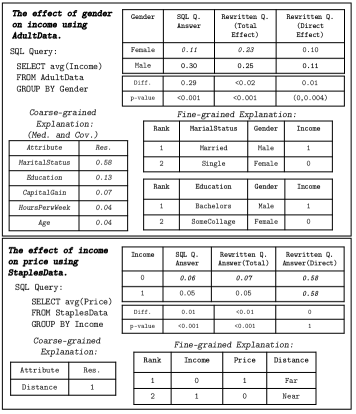
Figure 3: The effect of gender on income in AdultData (top); The effect of income on price in StaplesData (bottom).

[t!]

7.3 End-to-end results (Q2)

In the following experiments, for each query, the relevant covariates and mediators were detected using the CD algorithm with HyMIT (Sec. 6). Table. 1 reports the running times of the covariates detection. Some of the datasets used in this experiment also investigated by FairTest [57]. By using the same datasets, we could compare our results and confirm them.

AdultData. Using this dataset, several prior works in algorithmic fairness have reported gender discrimination based on a strong statistical dependency between income and gender in favor of males [27, 61, 57]. In particular, FairTest reports 11% of women have high income compared to 30% of men, which suggests a huge disparity against women. We applied HypDB to AdultData to compute the effect of gender on income. We started with the query in Fig. 3 (top), which computes the average of Income (1 iff Income> 50k) Group By Gender, which indeed suggests a strong disparity with respect to females’ income. Note that FairTest essentially reports the result of the query in Fig. 3 (top). In contrast, HypDB  detects that this query is biased. It identifies attributes, such as MaritalStatus, Education, Occupation and etc., as mediators and covariates. The result of the rewritten query suggests that the disparity between male and female is not nearly as drastic. The explanations generated by HypDB show that Maritalstatus accounts for most of the bias, followed by Education. However, the top fine-grained explanations for MaritalStatus reveal surprising facts: there are more married males in the data than married females, and marriage has a strong positive association with high income. It turns out that the income attribute in US census data reports the adjusted gross income as indicated in the individual’s tax forms, which depends on filing status (jointly and separately), could be household income. Thus, AdultData is inconsistent and should not be used to investigate gender discrimination. HypDB  explanations also show that males tend to have higher educations than females and higher educations is associated with higher incomes. Although, this dataset does not meet the assumptions needed for inferring causal conclusions, HypDB’s report is illuminating and goes beyond FairTest.

BerkeleyData. In 1973, UC Berkeley was sued for discrimination against females in graduate school admissions. The admission figures for the fall of 1973 showed that men applying were more likely than women to be admitted, and the difference was so large that it was unlikely to be due to chance. The result of the query in Fig. 4 (top) suggests a huge disparate impact on female applicants. However, the query is bias w.r.t. Department. After removing bias by rewriting the query, HypDB reveals that disparity between males and females is not nearly as drastic (Fig. 4 (top)). Note that potentially missing covariates, such as an applicant’s qualification, prohibits causal interpretation of the answers. However, the fine-grained explanations generated by HypDB are insightful. They reveal that females tended to apply to departments such as F that have lower acceptance rates, whereas males tended to apply to departments such as A and B that have higher acceptance rates. For BerkeleyData, FairTest reports a strong association between Gender and Acceptance, which becomes insignificant after conditioning on Department. In contrast, HypDB reveals that there still exists an association even after conditioning, but the trend is reversed! In addition, HypDB’s explanations demystify the seemingly paradoxical behavior of this dataset. These explanations agree with the conclusion of [5], in which the authors investigated BerkeleyData.

StaplesData. Wall Street Journal investigators showed that Staples’ online pricing algorithm discriminated against lower income people [59]. The situation was referred to as an “unintended consequence" of Staples’s seemingly rational decision to adjust online prices based on user proximity to competitors’ stores. We used HypDB to investigate the problem. As depicted in Fig 3 (bottom), HypDB reveals that Income has no direct effect on Price. However, it has an indirect effect via Distance. The explanations show that this is simply because people with low incomes tend to live far from competitors’ stores, and people who live far get higher prices. This is essentially the conclusion of [59]. For StaplesData, FairTest reports strong association between Income and Price, which is confirmed by HypDB. However, the obtained insights from HypDB, e.g., the indirect interaction of Income and Price, are more profound and critically important for answering the question whether the observed discrimination is intended or unintended.

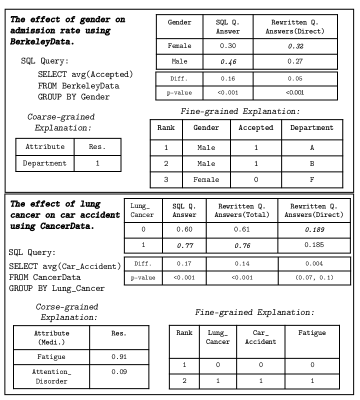
Figure 4: Report of the effect of lung cancer on car accident on CancerData (top); report of the effect of gender discrimination in BerkeleyData (bottom).

CancerData. This is a simulated dataset generated according to the causal DAG shown in Fig. 7 in the appendix. This data was used to test all three components of HypDB against ground truth. We used the query in Fig. 4 (bottom) to decide whether lung cancer has any impact on car accidents. According to the ground truth, there is no direct edge between lung cancer and car accidents; hence, there is no significant direct causal effect. However, since there is an indirect path between them, we expect a significant total causal effect. As shown in Fig. 4 (bottom), HypDB detects that this query is biased and correctly discovers sufficient confounding and mediator variables. The explanations for bias show that fatigue is the most responsible attribute for bias; people with lung cancer tend to be fatigued, which is highly associated with car accidents. Thus, the answers to the rewritten queries and explanations coincide with the ground truth.

FlightData. The results presented in Ex. 1.1 were generated using HypDB. During covariate detection, HypDB identifies and drops logical dependencies induced by attributes such as FlightNum, TailNum, AirportWAC, etc. It identified attributes such as Airport, Year, ArrDelay, Deptime, etc., as covariates and mediating variables. The generated explanations coincide with the intuition in Ex. 1.1.

Finally, we remark that the assumptions needed to perform parametric independence tests fail for FlightData and AdultData due to the large number of categories in their attributes and the high density of the underlying causal DAG; (this also justifies the higher running time for these datasets). The analysis of these datasets was possible only with the non-parametric tests developed in Sec 5. (Also, other CDD methods we discuss in the next section were not able to infer sufficient covariates and mediators.) To test the significance of $\hat{I}(T;Y|{\mathbf{Z}})$ with MIT, the permutation confidence interval was computed based on $m=100$ permutation samples. We restricted the test to a sample of groups of size proportional to $\log(|\Pi_{{\mathbf{Z}}}(D)|)$ as described in Sec. 5. Note that we used the significance level of 0.01 in all statistical tests in the CD algorithm.

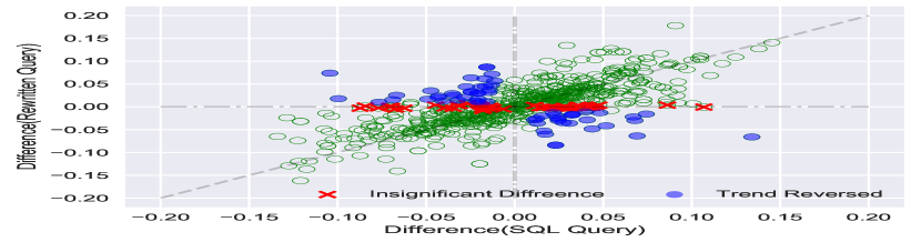
(a) The effect of query rewriting on FlightData.

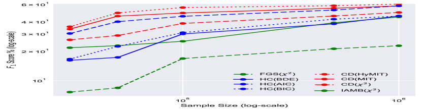
(b) Quality comparison.

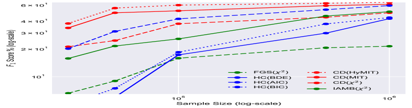
(c) Quality comparison for nodes with at least two parents.

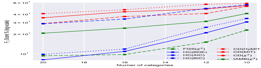
(d) Quality comparison with decreasing number of categories.

Figure 5: Results of the experiments.

7.4 Quality comparison (Q3)

We used RandomData, for which we had the ground truth, to assess the quality of the CD algorithm. We used the algorithm to learn the parents of all attributes in the corresponding DAG underlying different datasets in RandomData. We repeated the experiment with the following independence tests: MIT with sampling (same sampling fraction as in Sec 7.3), HyMIT and $\chi^{2}$. We used the F1-score as the accuracy metric to measure the performance the CD algorithm and compared it to the following reference algorithms implemented in the bnlearn library in R [33]: two contained-based methods, Full Grow-Shrink (FGS) [28] and Incremental Association (IAMB) [58] with $\chi^{2}$ independent test; the score based greedy search with Akaike Information Criterion (AIC), Bayesian Dirichlet equivalent (BDe) and Bayesian Information Criterion (BIC) scores. The significance level of 0.01 was used in all statistical tests.

The FGS utilizes Markov boundary for learning the structure of a causal DAG. It first discovers the Markov boundary of all nodes using the Grow-Shrink algorithm. Then, it determines the underlying undirected graph, which consists of all nodes and their neighbors. For edge orientation, it uses similar principles as used in the CD algorithm. The IAMB is similar to FGS except that it uses an improved version of the Grow-Shrink algorithm to learn Markov boundaries. Note that the superiority of CDD methods based on Markov boundary to other constraint-based method (such as the PC algorithm [56]) was shown in [45]. Thus, we restricted the comparison to these algorithms.

Fig. 5 (b) shows that our algorithm significantly outperforms most other algorithms. We remark, however, that this comparison is not fair, because the CD algorithm is not designed for learning the entire structure of a DAG. In fact, other constrained-based algorithms use the information across different nodes for edge origination. Thus, they could potentially learn the parent of a nodes with only one parent. Since learning the entire DAG is not the focus of our algorithm, in Fig. 5 (c) and (d) we restrict the comparison to nodes with at least two parents (either neighbors or not). As depicted, the CD algorithm with HyMIT outperforms all other algorithms. Notice that for smaller datasets and larger number of categories, our algorithm performs much better than the other algorithms. In fact, for a fixed DAG, $\chi^{2}$ test and score based methods become less reliable on sparse data. Conditioning on ${\mathbf{Z}}$ splits the data into $|\Pi_{{\mathbf{Z}}}(D)|$ groups. Thus, conditioning on large ${\mathbf{Z}}$ causes the data to split into very small groups that makes inference about independence less reliable. Fig. 5 (d) shows that , for sparse data, tests based on permutation deliver highest accuracy. Note that size conditioning sets in the CD algorithm depends on the density of underling causal DAGs. In Ex. 1.1, the largest conditioning set used by HypDB, consists of only 6 out of 101 attributes in FlightData.

An interesting observation is that even though our method uses principles that are similar to the other constraint-based methods, it outperforms them even with the same independence test, i.e., $\chi_{2}$ test. This is because the CD  algorithm uses a novel two-phase search strategy that optimized for learning parents, and does not relay on learning the underling undirected graph. As shown in Fig 6 (a), the CD algorithm conducted fewer independence tests per node than the FGS algorithm. Fewer independence tests not only improve efficiency but make the algorithm more reliable. Note that we only compared with the FGS, because we also used the Grow-Shrink algorithm to compute Markov boundaries. Also, notice that learning the parents of a nodes required many fewer independence test than the entire causal DAG. This makes our algorithm scalable to highly dimensional data for which learning the entire causal DAG is infeasible.

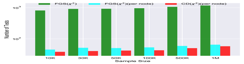
(a) Comparing the number of independence tests.

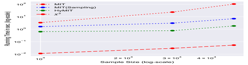
(b) Efficacy of the optimizations proposed for independence tests.

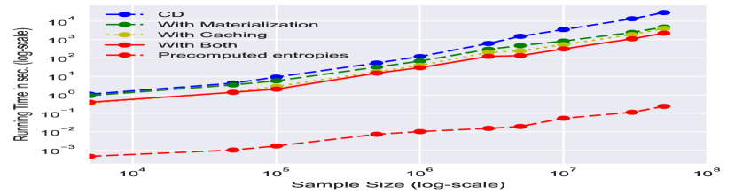
(c) Efficacy caching and materialization.

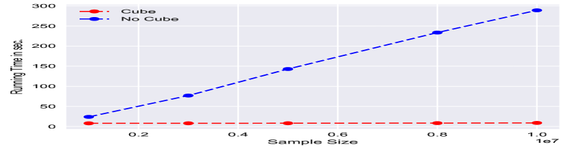
(d) Benefits of using data cubes.

Figure 6: Results of the experiments.

7.5 Efficacy of the optimization techniques (Q4)

To evaluate the quality of the optimizations proposed for non-parametric independence tests, we compared the running time and performance of MIT, MIT with sampling (same sampling fraction as in Sec 7.3), HyMIT and $\chi^{2}$ tests using the same data as used in Sec 7.4, but we restricted the experiments to samples smaller than 50k, to study their behavior on sparse data. Fig 6 (b) compares the average running time of performing each tests. As depicted, both MIT with sampling and HyMIT are much faster that MIT. Fig 8 (a), in the appendix, shows that the proposed tests have comparable accuracy. Note that HyMIT performs better than MIT with sampling, because it avoids sampling when $\chi^{2}$ test is applicable. Performing one permutation test with shuffling data consumes hours in the smallest dataset used in this experiment, whereas with MIT takes less than a second.

To evaluate the efficacy of materializing contingency tables and caching entropies, we used the same data as in Sec 7.4. As shown in Fig.  6 (c), both optimizations are effective. The efficacy of materializing contingency tables increases for larger sample sizes, because these tables becomes relatively much smaller than the size of data as the sample size increases. Note that we used pandas [30] to implement the statistical testing framework of HypDB. Computing entropies, which is essentially a group-by query, with pandas is up to 100 times slower than the same task in bnlearn. Fig.  6 (c) also shows the running time of the CD algorithm minus the time spent for computing entropies. As depicted, entropy computation constitutes the major computational effort in the CD algorithm.

Finally, we showed that computation of CD algorithm can benefit from pre-computed OLAP data-cubes and can be pushed inside a database engine. We used PostgreSQL to pre-compute data-cubes (with Count as measure) for RandomData with 8, 10 and 12 attributes. In Fig.  6 (d), we vary the input data size, whereas in Fig 8 (b), in the appendix, we vary the number of attributes. Both the graphs show that the advantage of using data-cube is dramatic. Note that the cube operator in PostgreSQL is restricted to 12 attributes. We also restrict to binary data for which computing a cube on the largest dataset used in this experiment took up to 30 hours. Without restricting to binary we could only compute a cube over a few number of attributes and small datasets.

8 Discussion and Related Work

Assumptions.

HypDB can detect, explain and resolve bias of a query under three assumptions: (1) parents of the treatment attributes in the underling causal DAG are included in data, (2) the treatment has at least two non-neighbor parents, and (3) The faithfulness assumption (see Sec. 10.1), which implies conditional independence implies no casual relationship. While drawing causal conclusions without (1) is impossible in general, there are techniques to handle unobserved attributes in certain cases [39], that can be incorporated in HypDB. Failure of (2) fundamentally prohibits the identification of the parents from observational data. Sec. 4 offers an agenda for future work to deal with such cases. The failure of (3) has been the subject of many (philosophical) discussions. However, it has been argued that in most practical settings this assumption is justifiable (see [35]).

Algorithmic fairness.

While it is known in causal inference that any claim of unfairness requires evidence of causality [38], most work in algorithmic fairness defines discrimination as strong statistical dependency between an algorithm’s outputs and protected attributes. For instance in legal dispute over hiring discrimination, neither the correlation between sex or race and hiring, nor their effect on applicant’s qualification, nor the effect of qualifications on hiring are target of investigation. Rather, to prove discrimination one must show that race or sex directly affect hiring decisions. Even though they may indirectly affect hiring by way of applicant qualification. In several experiments, we showed that one can use HypDB to detect unfairness post factum using simple SQL queries. HypDB reach for beyond state-of-the-art tools for fairness such as Fairtest [57].

Statistical Errors.

HypDB relies on conditional independent tests that are subject to false positives and false negatives. While it is generally impossible to absolutely prevent the two types of errors simultaneously, there are standard techniques to control for the false discovery rate in learning causal DAGs (e.g., [24]). We leave this extension for future work. The ramification of statistical errors in interpreting HypDB results can be summarized as follows: if HypDB reports no significant effect after rewriting a SQL query wrt. inferred covariates, then its answers are reliable under Faithfulness and if sufficient data is available, regardless of statistical errors and potential spurious attributes in the covarites. The reason is that the set of covariates at hand explains the spurious correlation reported by the SQL query. However, if the obtained effect after query rewriting is still significant, then in the presence of statistical errors, the answers could be unreliable.

OLAP Aspects.

More general OLAP queries e.g., queries with drill-down, roll-up or cube operator can be expressed as a set of group-by queries as studied in this paper. However, addressing the performance issues goes beyond the scope of this paper. In the context of causality, measures such as average treatment effect, likelihood ratios, analysis of variance (ANOVA) and information-theoretic metrics (such as mutual information) often used to quantify causal effect (see, [22]). HypDB can be extended to support these aggregates. Finally, the type of analysis proposed is this paper is not supported by OLAP data cubes. However, we showed that pre-computed cubes significantly speed up all components of HypDB. They rely on computing conditional probabilities or entropies that are GROUP BY count queries.

Simpson’s Paradox.

Prior research [9, 11, 13, 16], studied Simpson’s paradox in OLAP and data mining. They concerned with the efficient detection of instances of Simpson’s paradox as unexpected/surprising patterns in data. However, it is widely known in causal inference that such statistical anomalies neither reveal interesting facts in data nor are paradoxical [41]. They appear paradoxical once the result of biased queries is given causal interpretation and occur as a result of ignoring confounding variables.

Hypothetical Queries.

Much literature addresses hypothetical OLAP queries, e.g., [1, 23, 8]. They concerned with computing OLAP queries given a hypothetical scenario, which updates a database. Their approach, however is not adequate for data-driven decision making. Databases are the observed outcome of complicated stochastic processes in which the causal mechanism that determines the value of one variable interferes with those that determine others; hence, computing the effect of hypothetical updates requires knowledge about the causal interaction of variables. Thus, HypDB learns parts of the causal model relevant to a query at hand to account for confounding influences. Our future work includes extending HypDB to efficiently answer arbitrary “what-if" and “how-so" queries that drive actionable insights.

Causality in databases

The notion of causality has been studied extensively in databases [31, 48, 52, 53, 4, 3, 51]. We note that this line of work is different than the present paper in the sense that, it aims to identify causes for an observed output of a data transformation. For example, in query-answer causality/explanation, the objective is to identify parts of a database that explain a result of a query. While these works share some aspects of the notion of causality as studied in this paper, the problems that they address are fundamentally different. In [54] it has been shown that common inference problems in causality can be pushed into database system.

9 Conclusion

This paper proposed HypDB, a system to detect, explain, and resolve bias in decision-support OLAP queries. We showed that biased queries can be perplexing and lead to statistical anomalies, such as Simpson’s paradox. We proposed a novel technique to find explanations for the bias, thereby assisting the analyst in interpreting the results. We developed an automated method for rewriting the query into an unbiased query that correctly performs the hypothesis test that the analyst had in mind. The rewritten queries compute causal effects or the effect of hypothetical interventions. At the core of our framework lies the ability to find confounding variables. We showed that our method outperforms the state of the art causal DAG discovery methods. We showed that HypDB can be used to detect algorithmic unfairness post factum and the obtained insights go beyond state of the art e.g., Fairtest [57]. Our system can be used as an adhoc analysis along with OLAP data-cubes to detect, resolve and explain bias interactively at query time.

10 Appendix

10.1 Additional Background

We give here some more technical details to the material in Sec. 2.

Entropy

The entropy of a subset of random variables $\mathbf{X}\subseteq\mathbf{A}$ is $H(\mathbf{X})\stackrel{{\scriptstyle\text{def}}}{{=}}-\sum_{{\mathbf{x}}\in Dom({\mathbf{X}})}{\tt\mathrm{Pr}}({\mathbf{x}})\log{\tt\mathrm{Pr}}({\mathbf{x}})$, where ${\tt\mathrm{Pr}}({\mathbf{x}})$ is the marginal probability. The conditional mutual information (CMI) is $I(\mathbf{X};{\mathbf{Y}}|{\mathbf{Z}})\stackrel{{\scriptstyle\text{def}}}{{=}}H(\mathbf{X}{\mathbf{Z}})+H(\mathbf{X}{\mathbf{Y}})-H(\mathbf{X}{\mathbf{Z}}{\mathbf{Y}})+H({\mathbf{Z}})$. We say that $\mathbf{X}$, ${\mathbf{Y}}$ are conditionally independent (CI), in notation $\mathbf{X}\mbox{$\perp\!\!\!\perp$}{\mathbf{Y}}|{\mathbf{Z}}$, if $I(\mathbf{X};{\mathbf{Y}}|{\mathbf{Z}})=0$. Notice that all these quantities are defined in terms of the unknown population and the unknown probability ${\tt\mathrm{Pr}}(\mathbf{A})$. To estimate the entropy from the database $D$ we use the Miller-Madow estimator [32]: $\hat{H}(\mathbf{X})=\sum_{\mathbf{x}\in\Pi_{\mathbf{X}}(D)}F(\mathbf{x})\log F(\mathbf{x})+\frac{m-1}{2n}$, where $F(\mathbf{x})=\frac{1}{n}\sum_{\mathbf{a}\in D}1_{\mathbf{a}[\mathbf{X}]=\mathbf{x}}$ (the empirical distribution function) and $m=|\Pi_{\mathbf{X}}(D)|$ is the number of distinct elements of $\mathbf{X}$. We refer to the sample estimate of $I(\mathbf{X};{\mathbf{Y}}|{\mathbf{Z}})$ as $\hat{I}(\mathbf{X};{\mathbf{Y}}|{\mathbf{Z}})$.

Justification of Unconfoundedness

In the Neyman-Rubin Causal Model, the independence assumption states that $(Y(t_{0}),Y(t_{1})\mathrel{\text{\scalebox{1.07}{$\perp\mkern-10.0mu\perp$}}}T)$. This assumption immediately implies ${\tt\mathbb{E}}[Y(t_{i})]={\tt\mathbb{E}}[Y(t_{i})|T=t_{i}]$, $i=0,1$, and therefore ATE can be computed as:

$${\tt\textsc{ATE}}(T,Y)={\tt\mathbb{E}}[Y|T=t_{1}]-{\tt\mathbb{E}}[Y|T=t_{0}]$$ (6)

Here $Y$ is $Y(T)$, the attribute present in the data, and thus Eq. (2) can be estimated from $D$ as the difference of $\texttt{avg}(Y)$ for $T=t_{1}$ and for $T=t_{0}$. Notice that one should not to confuse the independence assumption $({Y(t_{0}),Y(t_{1})\mathrel{\text{\scalebox{1.07}{$\perp\mkern-10.0mu\perp$}}}T})$ with $({Y\mathrel{\text{\scalebox{1.07}{$\perp\mkern-10.0mu\perp$}}}T})$, meaning $({Y(T)\mathrel{\text{\scalebox{1.07}{$\perp\mkern-10.0mu\perp$}}}T})$; if the latter holds, then $T$ has no causal effect on $Y$. Under the independence assumption,

The independence assumption holds in randomized data (where the treatment $T$ is chosen randomly), but fails in observational data. In the case of observational data, we need to rely on the weaker Assumption 2.1. Notice that Unconfoundedness essentially states that the independence assumption holds for each value of the covariates. Thus, Eq.(6) holds once we condition on the covariates, proving the adjustment formula (2).

Causal DAGs

Intuitively, a causal DAG $G$ with nodes $V(G)=\mathbf{A}$, and edges $E(G)$ captures all potential causes between the variables [38, 39, 7]. We review here how compute the covariates ${\mathbf{Z}}$ using the DAG $G$, following [43]. A node $X_{i}$ is a parent of $X_{j}$ if $(X_{i},X_{j})\in E(G)$, ${\mathbf{PA}}_{X_{j}}$ denotes the set of parents of $X_{j}$, and two nodes $X_{i}$ and $X_{j}$ are neighbors if one of them is a parent of the other one. A path ${\mathbf{P}}$ is a sequence of nodes $X_{1},\ldots,X_{\ell}$ such that $X_{i}$ and $X_{i+1}$ are neighbors forall $i$. ${\mathbf{P}}$ is directed if $(X_{i},X_{i+1})\in E(G)$ forall $i$, otherwise it is nondirected. If there is a directed path from $X$ to $Y$ then we write $X\stackrel{{\scriptstyle*}}{{\rightarrow}}Y$, and we say $X$ is an ancestor, or a cause of $Y$, and $Y$ is a descendant or an effect of $X$. A nondirected path ${\mathbf{P}}=(X_{1},\ldots,X_{\ell})$ from $X_{1}$ to $X_{\ell}$ is called a back-door if $(X_{2},X_{1})\in E(G)$ and $(X_{\ell-1},X_{\ell})\in E(G)$. $X_{k}$ is a collider in a path ${\mathbf{P}}$ if both $X_{k-1}$ and $X_{k+1}$ are parents of $X_{k}$. A path with a collider is closed; otherwise it is open; note that an open path has the form $X\stackrel{{\scriptstyle*}}{{\leftarrow}}\stackrel{{\scriptstyle*}}{{\rightarrow}}Y$, i.e. $X$ causes $Y$ or $Y$ causes $X$ or they have a common cause. If ${\mathbf{P}}$ is open, then we say that a set of nodes ${\mathbf{Z}}$ closes ${\mathbf{P}}$ if ${{\mathbf{P}}}\cap{{\mathbf{Z}}}\neq\emptyset$. Given two sets of nodes ${\mathbf{X}},{\mathbf{Y}}$ we say that a set ${\mathbf{Z}}$ d-separates ${\mathbf{X}}$ and ${\mathbf{Y}}$, denoted by ${\mathbf{X}}\mbox{$\perp\!\!\!\perp$}{\mathbf{Y}}|_{d}\ {\mathbf{Z}}$, if ${\mathbf{Z}}$ closes every open path from ${\mathbf{X}}$ to ${\mathbf{Y}}$ [43]. This special handling of colliders, reflects a general phenomenon known as Berkson’s paradox, whereby conditioning on a common consequence of two independent cause render spurious correlation between them, see Ex. 10.1 below.

Example 10.1

CancerData [17] is a simulated dataset generated according to the causal DAG shown in Fig. 7. In this graph, Smoking is a collider in the path between Peer_Pressure and Anxiety, i.e., ${\mathbf{P}}$: Peer_Pressure $\rightarrow$ Smoking $\leftarrow$ Anxiety. Furthermore, ${\mathbf{P}}$ is the only path between Peer_Pressure and Anxiety. Since ${\mathbf{P}}$ is a closed path, Anxiety and Peer_Pressure are marginally independent. This independence holds in CancerData, since $I(\text{Anxiety},\text{Peer\_Pressure})=0.000004$, which is not statistically significant (pvalue>0.6). Now, since Smoking is a collider in ${\mathbf{P}}$, conditioning on Smoking renders spurious correlation between Anxiety and _Pressure. From CancerData we obtain that, $I(\text{Anxiety},\linebreak\text{Peer\_Pressure}|\text{Smoking})=0.003$, which is statistically significant (pvalue<0.001).

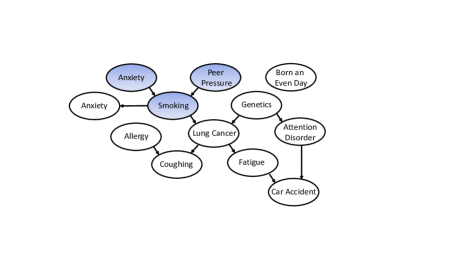
Figure 7: The causal DAG used to generate CancerData.

Definition 10.2

A distribution $\Pr({\mathbf{A}})$ on the variables ${\mathbf{A}}$ is causal or DAG-isomorphic if there exists a DAG $G$ with nodes ${\mathbf{A}}$ such that ${\mathbf{X}}\mbox{$\perp\!\!\!\perp$}{\mathbf{Y}}|_{d}\ {\mathbf{Z}}\Leftrightarrow{\mathbf{X}}\mbox{$\perp\!\!\!\perp$}{\mathbf{Y}}|{\mathbf{Z}}$ [42, 39, 56].

Fix a treatment $T$ and outcome $Y$. A set ${\mathbf{Z}}$ is said to satisfy the back-door criterion if it closes all back-door paths from $T$ to $Y$. Pearl [37] proved the following:

Theorem 10.3

[39, Th. 3.2.5] if ${\mathbf{Z}}$ satisfies the back-door criterion, then it satisfies Unconfoundedness.

Total and Direct Effects

ATE measures the total effect of $T$ on $Y$, aggregating over all directed paths from $T$ to $Y$. In some cases we want to investigate the direct effect, or natural direct effect, NDE [38], which measures the effect only through a single edge from $T$ to $Y$, which we review here. A node $M$ that belongs to some directed path from $T$ to $Y$ is called a mediator. We will assume that each unit in the population has two attributes $Y(t_{1})$ and $Y(t_{0},M(t_{1}))$, representing the outcome $Y$ when we apply the treatment $t_{1}$, and the outcome when we don’t apply the treatment and simultaneously keep the value of all mediators, ${\mathbf{M}}$, to what they were when the treatment $t_{1}$ was applied. Then:

$${\tt\textsc{NDE}}(T,Y)\stackrel{{\scriptstyle\text{def}}}{{=}}{\tt\mathbb{E}}[Y(t_{0},{\mathbf{M}}(t_{1}))]-{\tt\mathbb{E}}[Y(t_{1})]$$ (7)

For example, in gender discrimination the question is whether gender has any direct effect on income or hiring [38]. Here $t_{1}=$Male, $t_{0}=$Female, $Y$ is the decision to hire, while the mediators ${\mathbf{M}}$ are the qualifications of individuals. The outcome $Y(t_{0},M(t_{1}))$ is the hiring decision for a male, if we changed his gender to female, but kept all the qualifications unchanged. Since $Y(t_{0},M(t_{1}))$ is missing in the data, NDE can not be estimated, even with a controlled experiment [38]. However, for mediators ${\mathbf{M}}\stackrel{{\scriptstyle\text{def}}}{{=}}{\mathbf{PA}}_{Y}-\{T\}$ and covariates ${\mathbf{Z}}\stackrel{{\scriptstyle\text{def}}}{{=}}{\mathbf{PA}}_{T}$, it satisfies the mediator formula [38], given by Eq.(3) in Sec. 2.

10.2 Additional Proofs, Algorithms, Examples and Graphs

In this section we present some of the proofs and algorithms that were missing in the main part of the paper. We also present additional examples and graphs.

Proof of Prop.3.2

We prove (a) (the proof of (b) is similar and omitted). Denoting ${\mathbf{Y}}_{j}\stackrel{{\scriptstyle\text{def}}}{{=}}(Y_{j}(t_{0}),Y_{j}(t_{1}))$, we will prove independence in the context $\Gamma_{i}$, i.e. $({\mathbf{Y}}_{j}\mathrel{\text{\scalebox{1.07}{$\perp\mkern-10.0mu\perp$}}}T|\Gamma_{i})$. Using (1) unconfoundedness for ${\mathbf{Z}}$, $({\mathbf{Y}}_{j}\mathrel{\text{\scalebox{1.07}{$\perp\mkern-10.0mu\perp$}}}T|{\mathbf{Z}}={\mathbf{z}})$, and (2) the balanced assumption for $\mathcal{Q}$, $(T\mbox{$\perp\!\!\!\perp$}{\mathbf{Z}}|\Gamma_{i})$, we show: ${\tt\mathbb{E}}[T|{\mathbf{Y}}_{j}={\mathbf{y}},\Gamma_{i}]={\tt\mathbb{E}}_{{\mathbf{z}}}[{\tt\mathbb{E}}[T|{\mathbf{Y}}_{j}={\mathbf{y}},\Gamma_{i},{\mathbf{Z}}={\mathbf{z}}]|{\mathbf{Y}}_{j}={\mathbf{y}},\Gamma_{i}]={\tt\mathbb{E}}_{{\mathbf{z}}}[{\tt\mathbb{E}}[T|{\mathbf{Z}}={\mathbf{z}},\Gamma_{i}]|{\mathbf{Y}}_{j}={\mathbf{y}},\Gamma_{i}]$ (by (1)) $={\tt\mathbb{E}}_{{\mathbf{z}}}[{\tt\mathbb{E}}[T|\Gamma_{i}]|{\mathbf{Y}}_{j}={\mathbf{y}},\Gamma_{i}]$ (by (2)) $={\tt\mathbb{E}}[T|\Gamma_{i}]$ (because ${\tt\mathbb{E}}[T|\Gamma_{i}]$ is independent of ${\mathbf{z}}$), proving $({\mathbf{Y}}_{j}\mathrel{\text{\scalebox{1.07}{$\perp\mkern-10.0mu\perp$}}}T|\Gamma_{i})$.

Completing Example 1.1

Listing 3 shows the rewritten query associated to the biased query in Ex. 1.1. Query rewriting removes bias resulted from the influence of Airport, Year, Day and Month. See Sec. 3.3 for details.

Algorithm for Fine-Grained Explanations

The details of the procedure proposed in Sec. 3.2 for generating fine-grained explanations for a biased query is shown in Algorithm 3.

Additional Graphs

Figure 8 shows additional graphs for the experiments in Sec 7.5.

Listing 3: Rewritten query associated to Ex. 1.1.

⬇

WITH Blocks

AS(

SELECT Carrier,Airport,Year,Day,Month,avg(Delay) AS Avge

FROM FlightData

WHERE Carrier in (’AA’,’UA’) AND Airport in (’COS’,’MFE’,’MTJ’,’ROC’)

GROUP BY Carrier,Airport,Year,Day,Month),

Weights

AS(

SELECT Airport,Year,Day,Month, count(*)/n AS W

FROM FlightData

WHERE Carrier in (’AA’,’UA’) AND Airport in (’COS’,’MFE’,’MTJ’,’ROC’))

GROUP BY Airport,Year,Day,Month

HAVING count(DISTINCT Carrier)=2)

SELECT Carrier,sum(Avge * W)

FROM Blocks,Weights

WHERE Blocks.Airport = Weights.Airport AND

Blocks.Month = Weights.Month AND

Blocks.Day = Weights.Day AND

Blocks.Year = Weights.Year AND

GROUP BY Carrier

Input: A database $D$, three attributes $T,Y,Z\in\mathbf{A}$, an integer $k$ denotes the number of explanations

Output: Top-$k$ explanations

1

2${\mathbf{S}}\leftarrow\emptyset$

3

4for $(t,y,z)\in\Pi_{TYZ}(D)$ do

5       $K_{t}[(t,y,z)]\leftarrow\kappa_{(t,z)}$

6       $K_{y}[(t,y,z)]\leftarrow\kappa_{(y,z)}$

7      

8$R_{i}\leftarrow$ Rank $K_{i}$ by value, for $i\in\{t,y\}$

9 $R\leftarrow{\mathbf{RankAggregate}}(R_{t},R_{y})$

return Top-$k$ triples in $R$

Algorithm 3 Fine-Grained Explanation (FGE)

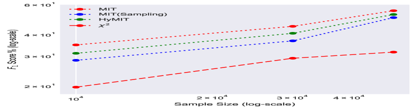
(a) Quality of the optimizations proposed for independence test.

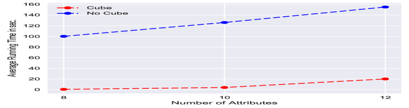
(b) Benefits of using data cubes.

Figure 8: Additional graphs for experiments in Sec. 7.

References

- [1] Andrey Balmin, Thanos Papadimitriou, and Yannis Papakonstantinou. Hypothetical queries in an olap environment. In VLDB, volume 220, page 231, 2000.
- [2] Nikolay Balov and Peter Salzman. How to use the catnet package, 2016.
- [3] Leopoldo Bertossi and Babak Salimi. Causes for query answers from databases: datalog abduction, view-updates, and integrity constraints. International Journal of Approximate Reasoning, 90:226–252, 2017.
- [4] Leopoldo Bertossi and Babak Salimi. From causes for database queries to repairs and model-based diagnosis and back. Theory of Computing Systems, 61(1):191–232, 2017.
- [5] Peter J Bickel, Eugene A Hammel, J William O’Connell, et al. Sex bias in graduate admissions: Data from berkeley. Science, 187(4175):398–404, 1975.
- [6] Carsten Binnig, Lorenzo De Stefani, Tim Kraska, Eli Upfal, Emanuel Zgraggen, and Zheguang Zhao. Toward sustainable insights, or why polygamy is bad for you. In CIDR, 2017.
- [7] Xavier De Luna, Ingeborg Waernbaum, and Thomas S Richardson. Covariate selection for the nonparametric estimation of an average treatment effect. Biometrika, page asr041, 2011.
- [8] Daniel Deutch, Zachary G Ives, Tova Milo, and Val Tannen. Caravan: Provisioning for what-if analysis. In CIDR, 2013.
- [9] Carem C Fabris and Alex A Freitas. Discovering surprising instances of simpson’s paradox in hierarchical multidimensional data. International Journal of Data Warehousing and Mining (IJDWM), 2(1):27–49, 2006.
- [10] Sheila R Foster. Causation in antidiscrimination law: Beyond intent versus impact. Hous. L. Rev., 41:1469, 2004.
- [11] Alex A Freitas. Understanding the crucial role of attribute interaction in data mining. Artificial Intelligence Review, 16(3):177–199, 2001.
- [12] Alex A Freitas. Are we really discovering interesting knowledge from data. Expert Update (the BCS-SGAI magazine), 9(1):41–47, 2006.
- [13] Clark Glymour, David Madigan, Daryl Pregibon, and Padhraic Smyth. Statistical themes and lessons for data mining. Data mining and knowledge discovery, 1(1):11–28, 1997.
- [14] Phillip Good. Permutation tests: a practical guide to resampling methods for testing hypotheses. Springer Science & Business Media, 2013.
- [15] Priscilla E Greenwood and Michael S Nikulin. A guide to chi-squared testing, volume 280. John Wiley & Sons, 1996.
- [16] Yue Guo, Carsten Binnig, and Tim Kraska. What you see is not what you get!: Detecting simpson’s paradoxes during data exploration. In Proceedings of the 2nd Workshop on Human-In-the-Loop Data Analytics, page 2. ACM, 2017.
- [17] Isabelle Guyon. Lung cancer simple model, 10 2009.
- [18] David Heckerman et al. A tutorial on learning with bayesian networks. Nato Asi Series D Behavioural And Social Sciences, 89:301–354, 1998.
- [19] Paul W Holland. Statistics and causal inference. Journal of the American statistical Association, 81(396):945–960, 1986.
- [20] Paul W. Holland. Statistics and causal inference. Journal of the American Statistical Association, 81(396):pp. 945–960, 1986.
- [21] Stefano M Iacus, Gary King, Giuseppe Porro, et al. Cem: software for coarsened exact matching. Journal of Statistical Software, 30(9):1–27, 2009.
- [22] Dominik Janzing, David Balduzzi, Moritz Grosse-Wentrup, and Bernhard Schölkopf. Quantifying causal influences. The Annals of Statistics, 41(5):2324–2358, 2013.
- [23] Laks VS Lakshmanan, Alex Russakovsky, and Vaishnavi Sashikanth. What-if olap queries with changing dimensions. In Data Engineering, 2008. ICDE 2008. IEEE 24th International Conference on, pages 1334–1336. IEEE, 2008.
- [24] Junning Li and Z Jane Wang. Controlling the false discovery rate of the association/causality structure learned with the pc algorithm. Journal of Machine Learning Research, 10(Feb):475–514, 2009.
- [25] M. Lichman. Uci machine learning repository, 2013.
- [26] Shili Lin. Rank aggregation methods. Wiley Interdisciplinary Reviews: Computational Statistics, 2(5):555–570, 2010.
- [27] Binh Thanh Luong, Salvatore Ruggieri, and Franco Turini. k-nn as an implementation of situation testing for discrimination discovery and prevention. In Proceedings of the 17th ACM SIGKDD international conference on Knowledge discovery and data mining, pages 502–510. ACM, 2011.
- [28] Dimitris Margaritis and Sebastian Thrun. Bayesian network induction via local neighborhoods. In Advances in neural information processing systems, pages 505–511, 2000.
- [29] John H McDonald. Handbook of biological statistics, volume 2. Sparky House Publishing, 2009.
- [30] Wes McKinney. pandas: a foundational python library for data analysis and statistics. Python for High Performance and Scientific Computing, pages 1–9, 2011.
- [31] Alexandra Meliou, Wolfgang Gatterbauer, Katherine F. Moore, and Dan Suciu. The complexity of causality and responsibility for query answers and non-answers. Proc. VLDB Endow. (PVLDB), 4(1):34–45, 2010.
- [32] George A Miller. Note on the bias of information estimates. Information theory in psychology: Problems and methods, 2(95):100, 1955.
- [33] Radhakrishnan Nagarajan, Marco Scutari, and Sophie Lèbre. Bayesian networks in r. Springer, 122:125–127, 2013.
- [34] Richard E Neapolitan et al. Learning bayesian networks, volume 38. Pearson Prentice Hall Upper Saddle River, NJ, 2004.
- [35] Eric Neufeld and Sonje Kristtorn. Whether non-correlation implies non-causation. In FLAIRS Conference, pages 772–777, 2005.
- [36] WM Patefield. Algorithm as 159: an efficient method of generating random r c tables with given row and column totals. Journal of the Royal Statistical Society. Series C (Applied Statistics), 30(1):91–97, 1981.
- [37] Judea Pearl. [bayesian analysis in expert systems]: Comment: Graphical models, causality and intervention. Statistical Science, 8(3):266–269, 1993.
- [38] Judea Pearl. Direct and indirect effects. In Proceedings of the seventeenth conference on uncertainty in artificial intelligence, pages 411–420. Morgan Kaufmann Publishers Inc., 2001.
- [39] Judea Pearl. Causality. Cambridge university press, 2009.
- [40] Judea Pearl. An introduction to causal inference. The international journal of biostatistics, 6(2), 2010.
- [41] Judea Pearl. Simpson’s paradox: An anatomy. Department of Statistics, UCLA, 2011.
- [42] Judea Pearl. Probabilistic reasoning in intelligent systems: networks of plausible inference. Morgan Kaufmann, 2014.
- [43] Judea Pearl et al. Causal inference in statistics: An overview. Statistics Surveys, 3:96–146, 2009.
- [44] Dino Pedreshi, Salvatore Ruggieri, and Franco Turini. Discrimination-aware data mining. In Proceedings of the 14th ACM SIGKDD international conference on Knowledge discovery and data mining, pages 560–568. ACM, 2008.
- [45] Jean-Philippe Pellet and André Elisseeff. Using markov blankets for causal structure learning. Journal of Machine Learning Research, 9(Jul):1295–1342, 2008.
- [46] Dataset: Airline On-Time Performance. http://www.transtats.bts.gov/.
- [47] Clark Glymour Peter Spirtes and Richard Scheines. Causation, Prediction and Search. MIT Press, 2001.
- [48] Sudeepa Roy and Dan Suciu. A formal approach to finding explanations for database queries. In Proceedings of the 2014 ACM SIGMOD international conference on Management of data, pages 1579–1590. ACM, 2014.
- [49] Donald B Rubin. The Use of Matched Sampling and Regression Adjustment in Observational Studies. Ph.D. Thesis, Department of Statistics, Harvard University, Cambridge, MA, 1970.
- [50] Donald B Rubin. Statistics and causal inference: Comment: Which ifs have causal answers. Journal of the American Statistical Association, 81(396):961–962, 1986.
- [51] Babak Salimi. Query-Answer Causality in Databases and its Connections with Reverse Reasoning Tasks in Data and Knowledge Management. PhD thesis, Carleton University, 2015.
- [52] Babak Salimi, Leopoldo Bertossi, Dan Suciu, and Guy Van den Broeck. Quantifying causal effects on query answering in databases. In TaPP, 2016.
- [53] Babak Salimi and Leopoldo E. Bertossi. From causes for database queries to repairs and model-based diagnosis and back. In ICDT, pages 342–362, 2015.
- [54] Babak Salimi, Corey Cole, Dan RK Ports, and Dan Suciu. Zaliql: causal inference from observational data at scale. Proceedings of the VLDB Endowment, 10(12):1957–1960, 2017.
- [55] Babak Salimi, Johannes Gehrke, and Dan Suciu. Bias in olap queries: Detection, explanation, and removal. In Proceedings of the 2018 International Conference on Management of Data, pages 1021–1035. ACM, 2018.
- [56] Peter Spirtes, Clark N Glymour, and Richard Scheines. Causation, prediction, and search. MIT press, 2000.
- [57] Florian Tramer, Vaggelis Atlidakis, Roxana Geambasu, Daniel Hsu, Jean-Pierre Hubaux, Mathias Humbert, Ari Juels, and Huang Lin. Fairtest: Discovering unwarranted associations in data-driven applications. In Security and Privacy (EuroS&P), 2017 IEEE European Symposium on, pages 401–416. IEEE, 2017.
- [58] Ioannis Tsamardinos, Constantin F Aliferis, Alexander R Statnikov, and Er Statnikov. Algorithms for large scale markov blanket discovery. In FLAIRS conference, volume 2, pages 376–380, 2003.
- [59] Jennifer Valentino-Devries, Jeremy Singer-Vine, and Ashkan Soltani. Websites vary prices, deals based on users’ information. Wall Street Journal, 10:60–68, 2012.
- [60] Rich Zemel, Yu Wu, Kevin Swersky, Toni Pitassi, and Cynthia Dwork. Learning fair representations. In Proceedings of the 30th International Conference on Machine Learning (ICML-13), pages 325–333, 2013.
- [61] Indre Žliobaite, Faisal Kamiran, and Toon Calders. Handling conditional discrimination. In Data Mining (ICDM), 2011 IEEE 11th International Conference on, pages 992–1001. IEEE, 2011.