Weighted Bayesian Bootstrap for Scalable Bayes

Abstract

We develop a weighted Bayesian Bootstrap (WBB) for machine learning and statistics. WBB provides uncertainty quantification by sampling from a high dimensional posterior distribution. WBB is computationally fast and scalable using only off-the-shelf optimization software such as TensorFlow. We provide regularity conditions which apply to a wide range of machine learning and statistical models. We illustrate our methodology in regularized regression, trend filtering and deep learning. Finally, we conclude with directions for future research.

Keywords: Bayesian, Bootstrap, MCMC, Weighted Bootstrap, ABC, Trend Filtering, Deep Learning, TensorFlow, Regularization.

1 Introduction

Weighted Bayesian Bootstrap (WBB) is a simulation-based algorithm for assessing uncertainty in machine learning and statistics. Uncertainty quantification (UQ) is an active area of research, particularly in high-dimensional inference problems. Whilst there are computationally fast and scalable algorithms for training models in a wide variety of contexts, uncertainty assessment is still required. Developing computationally fast scalable algorithms for sampling a posterior distribution is a notoriously hard problem. WBB makes a contribution to this literature by showing how off-the-shelf optimization algorithms, such as convex optimization or stochastic gradient descent (SGD) in TensorFlow can also be used to provide uncertainty quantification.

Our work builds on Newton and Raftery (1994) who provide a weighted likelihood Bootstrap (WLB) method for Bayesian inference. They develop a weighted likelihood Bootstrap algorithm together with the appropriate asymptotic analysis to show that such an algorithm provides efficient posterior samples. Their bootstrap procedure exploits the fact that the posterior distribution centered at the maximum likelihood estimate (MLE) has a second order expansion that also depends on the prior and its derivative. The weighted Bayesian Bootstrap (WBB) calculates a series of posterior modes rather than MLEs. This has the advantage that high dimensional posterior modes are readily available particularly using the regularized estimates are fast to compute from convex optimization methods or stochastic gradient descent (SGD) for neural network architectures such as deep learning. By linking WLB and WBB, with modern-day optimization to calibrate estimate, we provide a framework for uncertainty quantification.

Uncertainty estimates are provided at little to no extra cost. Quantifying uncertainty is typically unavailable in a purely regularization optimization method. Another feature that is straightforward to add is a regularization path across hyper-parameters. This is so much easier than traditional Bayesian to do prior sensitivity analysis where hyper-parameters are hard to assess. Rather we use predictive cross-validation techniques.

The rest of the paper is outlined as follows. Section 2 develops our weighted Bayesian Bootstrap (WBB) algorithm. Section 3 provides an application to high dimensional sparse regression, trend filtering and deep learning. WBB can also be applied to Bayesian tree models (Taddy et al. (2015)). Finally, Section 4 concludes with directions for future research. Areas for future study include Bootstrap filters in state-space models (Gordon et al. (1993)) and comparison with the resampling-sampling perspective to sequential Bayesian inference (Lopes et al. (2012)), etc.

2 Weighted Bayesian Bootstrap

Let $y$ an $n$-vector of outcomes, $\theta$ denotes a $d$-dimensional parameter of interest and $A$ a fixed $n\times d$ matrix whose rows are the design points (or “features”) $a_{i}^{T}$ where we index observations by $i$ and parameters by $j$. A large number of machine learning and statistical problems can be expressed in the form

$$\underset{\theta\in\mathcal{R}^{d}}{\text{minimize}} l(y|\theta)+\lambda\phi(\theta)\,,$$ (1)

where $l(y|\theta)=\sum_{i=1}^{n}\log f(y_{i};a_{i}^{\top}\theta)$ is a measure of fit (or “empirical risk function”) depending implicitly on $A$ and $y$. The penalty function or regularization term, $\lambda\phi(\theta)$, effects a favorable bias-variance tradeoff. We allow for the possibility that $\phi(\theta)$ may have points in its domain where it fails to be differentiable.

Suppose that we observe data, $y=(y_{1},\ldots,y_{n})$ from a model parameterized by $\theta$. For example, we might have a probabilistic model that depends on a parameter, $\theta$, where $p(y|\theta)$ is known as the likelihood function. Equivalently, we can define a measure of fit $l(y|\theta)=\log f(y;\theta)=\log p(y|\theta)$. We will make use of the following

1. Let $\hat{\theta}_{n}\mathrel{\mathop{:}}={\rm argmax}_{\theta}\;p(y|\theta)$ be the MLE,

2. Let $\theta^{*}_{n}\mathrel{\mathop{:}}={\rm argmax}_{\theta}\;p(\theta|y)$ be the posterior mode,

3. Let $\bar{\theta}_{n}\mathrel{\mathop{:}}=E(\theta|y)$ be the posterior mean.

We now develop a key duality between regularization and posterior bootstrap simulation.

2.1 Bayesian Regularization Duality

From the Bayesian perspective, the measure of fit, $l(y|\theta)=-\log f(y;\theta)$, and the penalty function, $\lambda\phi(\theta)$, correspond to the negative logarithms of the likelihood and prior distribution in the hierarchical model

$$f(y;\theta)=p(y|\theta)\propto\exp \{-l(y|\theta)\}\;,\quad p(\theta)\propto\exp\{-\lambda\phi(\theta)\}$$

$$p(\theta|y) \propto\exp\{-(l(y|\theta)+\lambda\phi(\theta))\}.$$

The prior is not necessarily proper but the posterior, $p(\theta|y)\propto p(y|\theta)p(\theta)$, may still be proper. This provides an equivalence between regularization and Bayesian methods. For example, regression with a least squares log-likelihood subject to a penalty such as an $L^{2}$-norm (ridge) Gaussian probability model or $L^{1}$-norm (lasso) double exponential probability model. We then have

$$\hat{\theta}_{n}= \underset{\theta\in\Theta}{\operatorname*{arg\,min}}\,l(y|\theta),$$ (2)

$$\theta^{*}_{n}= \underset{\theta\in\Theta}{\operatorname*{arg\,min}}\,\{l(y|\theta)+\lambda\phi(\theta)\}.$$ (3)

Let $\partial$ be the subdifferential operator. Then a necessary and sufficient condition for $\theta^{*}$ to minimize $l(y|\theta)+\lambda\phi(\theta)$ is

$$0\in\partial\left\{l(y|\theta)+\lambda\phi(\theta)\right\}=\nabla l(y|\theta)+\lambda\partial\phi(\theta)$$ (4)

the sum of a point and a set. The optimization literature characterizes $\theta^{*}$ as the fixed point of a proximal operator $\theta^{*}=\mathop{\mathrm{prox}}_{\gamma\phi}\{\theta^{*}-\lambda\nabla f(\theta^{*})\}$, see Polson and Scott (2015) and Polson, Scott, and Willard (2015) for further discussion.

A general class of natural exponential family models can be expressed in terms of the Bregman divergence of the dual of the cumulant transform. Let $\phi$ be the conjugate Legendre transform of $\psi$. Hence $\psi(\theta)=\sup_{\mu}\;\left(\mu^{\top}\theta-\phi(\mu)\right)$. Then we can write

$$p_{\psi}(y|\theta) =\exp\left(y^{\top}\theta-\psi(\theta)-h_{\psi}(y)\right)$$

$$=\exp\left\{\inf_{\mu}\;\left((y-\mu)^{\top}\theta-\phi(\mu)\right)-h_{\psi}(y)\right\}$$

$$=\exp\left(-D_{\phi}(y,\mu(\theta))-h_{\phi}(y)\right)$$

where the infimum is attained at $\mu(\theta)=\phi^{\prime}(\theta)$ is the mean of the exponential family distribution. We rewrite $h_{\psi}(y)$ is terms of the correction term and $h_{\phi}(y)$. Here there is a duality as $D_{\phi}$ can be interpreted as a Bregman divergence.

For a wide range of non-smooth objective functions/statistical models, recent regularization methods provide fast, scalable algorithms for calculating estimates of the form (3), which can also be viewed as the posterior mode. Therefore as $\lambda$ varies we obtain a full regularization path as a form of prior sensitivity analysis.

Strawderman et al. (2013) and Polson et al. (2015) considered scenarios where posterior modes can be used as posterior means from augmented probability models. Moreover, in their original foundation of the Weighted Likelihood Bootstrap (WLB), Newton and Raftery (1994) introduced the concept of the implicit prior. Clearly this is an avenue for future research.

2.2 WBB Algorithm

We now define the weighted Bayesian Bootstrap (WBB). Following Newton and Raftery (1994), we construct a randomly weighted posterior distribution denoted by

$${\bf w}=(w_{1},...,w_{n},w_{p}),\,p_{\bf w}(\theta|y)\propto\prod_{i=1}^{n}p(y_{i}|\theta)^{w_{i}}p(\theta)^{w_{p}}$$

where the weights $w_{p},w_{i}\sim Exp(1)$ are randomly generated weights. It’s equivalent to draw $w_{i}=\log(1/U_{i})$ where $U_{i}$’s are i.i.d. Uniform (0,1), which is motivated by the uniform Dirichlet distribution for multinomial data. We have used the fact that for i.i.d. observations, the likelihood can be factorized as $p(y|\theta)=\prod_{i=1}^{n}p(y_{i}|\theta)$. This is not crucial for our analysis but is a common assumption. Let $\theta^{*}_{{\bf w},n}$ denote the mode of this regularized distribution. Again, there is an equivalence

$$\theta^{*}_{{\bf w},n}:=\underset{\theta}{\operatorname*{arg\,max}}\;p_{\bf w}(\theta|y)\equiv\underset{\theta}{\operatorname*{arg\,min}}\sum_{i=1}^{n}w_{i}l_{i}(y_{i}|\theta)+\lambda w_{p}\phi(\theta)$$

where $l_{i}(y_{i}|\theta)=-\log p(y_{i}|\theta)$ and $\lambda\phi(\theta)=-\log p(\theta)$. Note that we have a weighted likelihood and a new regularization parameter, $\lambda w_{p}$.

The crux of our procedure is to create a sample of the weighted posterior modes $\{\theta_{{\bf w},n}^{*}\}$ (computationally cheap as each sub-problem can be solved via optimization). Our main result is the following:

Algorithm: Weighted Bayesian Bootstrap (WBB)

1. Iterate: sample ${\bf{w}}=\{w_{1},w_{2},...,w_{n},w_{p}\}$ via exponentials. $w_{p},w_{i}\sim Exp(1)$.

2. For each ${\bf{w}}$, solve $\theta^{*}_{{\bf w},n}=\underset{\theta}{\operatorname*{arg\,min}}\sum_{i=1}^{n}w_{i}l_{i}(\theta)+\lambda w_{p}\phi(\theta)$.

The WBB algorithm is fast and scalable to compute a regularized estimator. For a large number of popular priors, the minimizing solution $\theta^{*}_{{\bf w},n}$ in the second step can be directly obtained via regularization packages such as glmnet by Trevor Hastie and genlasso by Taylor Arnold. When the likelihood function or the prior is specially designed, Stochastic Gradient Descent (SGD) is powerful and fast enough to solve the minimization problem. It can be easily implemented in TensorFlow once the objective function is specified. See Appendix (A) and Polson and Sokolov (2017) for further discussion.

The next section builds on Newton and Raftery (1994) and derives asymptotic properties of the weighted Bayesian Bootstrap. We simply add the regularized factor. To choose the amount of regularization $\lambda$, we can use the marginal likelihood $m_{\lambda}(y)$, estimated by bridge sampling (Gelman and Meng (1998)) or simply using predictive cross-validation.

2.3 WBB Properties

The following proposition which follows from the Theorem 2 in Newton and Raftery (1994) summaries the properties of WBB.

Proposition The weighted Bayesian Bootstrap draws are approximate posterior samples

$$\left\{\theta^{*(k)}_{{\bf w},n}\right\}_{k=1}^{K}\sim p(\theta|y).$$

Now we consider ‘large $n$’ properties. The variation in the posterior density $p(\theta|y)\propto e^{-nl_{n}(\theta)}p(\theta)$ for sufficiently large $n$ will be dominated by the likelihood term. Expanding $l_{n}(\theta)$ around its maximum, $\hat{\theta}$, and defining $J_{n}(\hat{\theta})=nj(\hat{\theta})$ as the observed information matrix gives the traditional normal approximation for the posterior distribution

$$\theta\sim N_{d}\left(\hat{\theta}_{n},J_{n}^{-1}(\hat{\theta})\right)$$

where $\hat{\theta}_{n}$ is the MLE. A more accurate approximation is obtained by expanding around the posterior mode, $\theta^{*}$, which we will exploit in our weighted Bayesian Bootstrap. Now we have the asymptotic distributional approximation

$$\theta\sim N_{d}\left(\theta^{*},J_{n}^{-1}(\theta^{*})\right)$$

where $\theta^{*}_{n}\mathrel{\mathop{:}}={\rm arg\;max}_{\theta}\;p(\theta|y)$ is the posterior mode.

The use of the posterior mode here is crucially important as it’s the mode that is computationally available from TensorFlow and Keras. Approximate normality and second order approximation also holds, see Johnson (1970), Bertail and Lo (1991) and Newton and Raftery (1994) for future discussion. Specifically,

$$\sqrt{nI(\hat{\theta}_{n})}\left({\theta}^{*}_{n}-\hat{\theta}_{n}\right)\stackrel{{\scriptstyle D}}{{=}}Z$$

where $Z\sim N(0,1)$ is a standard Normal variable. The conditional posterior satisfies $\mathbb{P}\left(|{\theta}^{*}_{n}-\hat{\theta}_{n}|>\epsilon\right)\rightarrow 0$ for each $\epsilon>0$ as $n\rightarrow\infty$. In the ’large $p$’ case, a number of results are available for posterior concentration, for example, see Van Der Pas et al. (2014) for sparse high dimensional models.

3 Applications

Consider now a number of scenarios to assess when WBB corresponds to a full Bayesian posterior distribution.

3.1 Lasso

First, a simple univariate normal means problem with a lasso prior where

$$y|\theta\sim N(\theta,1^{2}),\quad\theta\sim Laplace(0,1/\lambda)$$

Given the i.i.d. exponential weights $w_{1}$ and $w_{2}$, the weighted posterior mode $\theta^{*}_{\bf w}$ is

$$\theta^{*}_{\bf w}=\underset{\theta\in\Theta}{\operatorname*{arg\,min}}\,\left\{\frac{w_{1}}{2}(y-\theta)^{2}+\lambda w_{2}|\theta|\right\}.$$

This is sufficiently simple for an exact WBB solution in terms of soft thresholding:

$$\theta^{*}_{\bf w}=\begin{cases}y-\lambda w_{2}/w_{1}&\mbox{if $y>\lambda w_{2}/w_{1}$},\\ y+\lambda w_{2}/w_{1}&\mbox{if $y<-\lambda w_{2}/w_{1}$},\\ 0&\mbox{if $|y|\leq\lambda w_{2}/w_{1}$}.\\ \end{cases}$$

The WBB mean $E_{{\bf w}}(\theta^{*}_{\bf w}|y)$ is approximated by the sample mean of $\{\theta^{*(k)}_{\bf w}\}_{k=1}^{K}$. On the other hand, Mitchell (1994) gives the expression for the posterior mean,

$$E(\theta|y) = \frac{\int_{-\infty}^{\infty}\theta\exp\left\{-(y-\theta)^{2}/2-\lambda|\theta|\right\}d\theta}{\int_{-\infty}^{\infty}\exp\left\{-(y-\theta)^{2}/2-\lambda|\theta|\right\}d\theta}$$

$$= \frac{F(y)}{F(y)+F(-y)}(y+\lambda)+\frac{F(-y)}{F(y)+F(-y)}(y-\lambda)$$

$$= y+\frac{F(y)-F(-y)}{F(y)+F(-y)}\lambda$$

where $F(y)=\exp(y)\Phi(-y-\lambda)$ and $\Phi(\cdot)$ is the c.d.f. of standard normal distribution. We plot the WBB mean versus the exact posterior mean in Figure (1). Interestingly, WBB algorithm gives sparser posterior means.

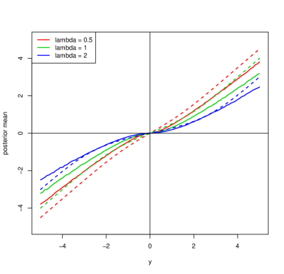
Figure 1: Normal means model with lasso prior: WBB mean $E_{{\bf w}}(\theta^{*}_{\bf w}|y)$ (in solid lines) versus exact posterior mean $E(\theta|y)$ (in dashed lines).

3.2 Diabetes Data

To illustrate our methodology, we use weighted Bayesian Bootstrap (WBB) on the classic diabetes dataset. The measurements for 442 diabetes patients are obtained ($n=442$), with 10 baseline variables ($p=10$), such as age, sex, body mass index, average blood pressure, and six blood serum measurements.

The likelihood function is given by

$$l(y|\beta)=\prod_{i=1}^{n}p(y_{i}|\beta)$$

where

$$p(y_{i}|\beta)=\frac{1}{\sqrt{2\pi}\sigma}\exp\left\{-\frac{1}{2\sigma^{2}}(y_{i}-x_{i}^{\prime}\beta)^{2}\right\}.$$

We draw 1000 sets of weights ${\bf{w}}=\{w_{i}\}_{i=1}^{n+1}$ where $w_{i}$’s are i.i.d. exponentials. For each weight set, the weighted Bayesian estimate $\beta^{*}_{\bf w}$ is calculated using (5) via the regularization method in the package glmnet.

$$\hat{\beta}_{\bf{w}}:=\underset{\beta}{\operatorname*{arg\,min}}\;\sum_{i=1}^{n}w_{i}(y_{i}-x_{i}^{\prime}\beta)^{2}+\lambda w_{n+1}\sum_{j=1}^{p}|\beta_{j}|\;.$$ (5)

The regularization factor $\lambda$ is chosen by cross-validation with unweighted likelihood. The weighted Bayesian Bootstrap is also performed with fixed prior, namely, $w_{n+1}$ is set to be 1 for all bootstrap samples. Polson et al. (2014) analyze the same dataset using the Bayesian Bridge estimator and suggest MCMC sampling from the posterior.

To compare our WBB results we also run the Bayesian bridge estimation. Here the Bayesian setting we use is

$$p(\beta,\sigma^{2})=p(\beta|\sigma^{2})p(\sigma^{2}),\,\text{where }p(\sigma^{2})\propto 1/\sigma^{2}.$$

The prior on $\beta$, with suitable normalization constant $C_{\alpha}$, is given by

$$p(\beta)=C_{\alpha}\exp(-\sum_{j=1}^{p}|\beta_{j}/\tau|^{\alpha}).$$

The hyper-parameter is drawn as $\nu=\tau^{-\alpha}\sim\Gamma(2,2)$, where $\alpha=1/2.$

Figure 2: Diabetes example: the weighted Bayesian Bootstrap (with fixed prior and weighted prior) and Bayesian Bridge are used to draw from the marginal posteriors for $\beta_{j}$’s, j = 1,2,…10.

Figure (2) shows the results of all these three methods (the weighted Bayesian Bootstrap with fixed prior / weighted prior and the Bayesian Bridge). Marginal posteriors for $\beta_{j}$’s are presented. One notable feature is that the weighted Bayesian Bootstrap tends to introduce more sparsity than Bayesian Bridge does. For example, the weighted Bayesian Bootstrap posteriors of age, ldl and tch have higher spikes located around 0, compared with the Bayesian Bridge ones. For tc, hdl, tch and glu, multi-modes in the marginal posteriors are observed. In general, the posteriors with fixed priors are more concentrated than those with randomly weighted priors. This difference is naturally attributed to the certainty in the prior weights.

3.3 Trend Filtering

The generalized lasso solves the optimization problem:

$$\beta^{*} = \underset{\beta}{\operatorname*{arg\,min}}\,\left\{l(y|\beta)+\lambda\phi(\beta)\right\}$$ (6)

$$= \underset{\beta}{\operatorname*{arg\,min}}\,\frac{1}{2}\|y-X\beta\|_{2}^{2}+\lambda\|D\beta\|_{1}$$ (7)

where $l(y|\beta)=\frac{1}{2}\|y-X\beta\|_{2}^{2}$ is the negative log-likelihood. $D\in\mathcal{R}^{m\times p}$ is a penalty matrix and $\lambda\phi(\beta)=\lambda\|D\beta\|_{1}$ is the negative log-prior or regularization penalty. There are fast path algorithms for solving this problem (see genlasso package).

As a subproblem, polynomial trend filtering (Tibshirani (2014); Polson and Scott (2015)) is recently introduced for piece-wise polynomial curve-fitting, where the knots and the parameters are chosen adaptively. Intuitively, the trend-filtering estimator is similar to an adaptive spline model: it penalizes the discrete derivative of order $k$, resulting in piecewise polynomials of higher degree for larger $k$.

Specifically, $X=I_{p}$ in the trend filtering setting and the data $y=(y_{1},...,y_{p})$ are assumed to be meaningfully ordered from 1 to $p$. The penalty matrix is specially designed by the discrete $(k+1)$-th order derivative,

$$D^{(1)}=\begin{bmatrix}-1&1&0&\dots&0&0\\ 0&-1&1&\dots&0&0\\ {5}\\ 0&0&0&\dots&-1&1\end{bmatrix}_{(p-1)\times p}$$

and $D^{(k+1)}=D^{(1)}D^{(k)}$ for $k=1,2,3...$. For example, the log-prior in linear trend filtering is explicitly written as $\lambda\sum_{i=1}^{p-2}|\beta_{i+2}-2\beta_{i+1}+\beta_{i}|$. For a general order $k>1$,

$$\|D^{(k+1)}\beta\|_{1}=\sum_{i=1}^{p-k-1}\Big{|}\sum_{j=i}^{i+k+1}(-1)^{(j-i)}\binom{k+1}{j-i}\beta_{j}\Big{|}.$$

WBB solves the following generalized lasso problem in each draw:

$$\beta_{\bf w}^{*} = \underset{\beta}{\operatorname*{arg\,min}}\,\frac{1}{2}\sum_{i=1}^{p}w_{i}(y_{i}-\beta_{i})^{2}+\lambda w_{p+1}\|D^{(k)}\beta\|_{1}$$

$$= \underset{\beta}{\operatorname*{arg\,min}}\,\frac{1}{2}\|Wy-W\beta\|_{2}^{2}+\lambda\|D^{(k)}\beta\|_{1}$$

$$= W^{-1}\underset{\tilde{\beta}}{\operatorname*{arg\,min}}\,\frac{1}{2}\|\tilde{y}_{\bf w}-\tilde{\beta}_{\bf w}\|_{2}^{2}+\lambda\|\tilde{D}^{(k)}_{\bf w}\tilde{\beta}_{\bf w}\|_{1}$$

where

$$W=diag(\sqrt{w_{i}}/\sqrt{w_{p+1}},...,\sqrt{w_{p}}/\sqrt{w_{p+1}})$$

and

$$\tilde{y}_{\bf w}=Wy,\,\tilde{\beta}_{\bf w}=W\beta,\,\tilde{D}^{(k)}_{\bf w}=D^{(k)}W^{-1}.$$

To illustrate our method, we simulate data $y_{i}$ from a Fourier series regression

$$y_{i}=\sin\left(\frac{4\pi}{500}i\right)\exp\left({\frac{3}{500}i}\right)+\epsilon_{i}$$

for $i=1,2,...500$, where $\epsilon_{i}\sim N(0,2^{2})$ are i.i.d. Gaussian noises. The cubic trend filtering result is given in Figure (3).

For each $i$, the weighted Bayesian Bootstrap gives a group of estimates $\left\{\beta_{\bf w}^{*}(i)\right\}_{j=1}^{T}$ where $T$ is the total number of draws. The standard error of $\hat{\beta}_{i}$ is easily computed using these weighted bootstrap estimates.

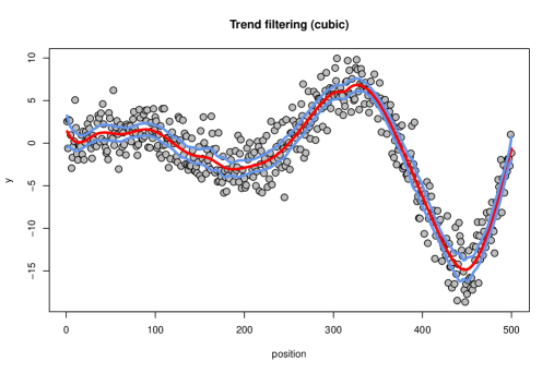
Figure 3: Cubic trend filtering: the red line is $\hat{\beta}_{i}$ for $i=1,2,...500$; the blue line is $\hat{\beta}_{i}\pm 2*se$ where the standard errors are easily computed by WBB. $\lambda=1000$.

3.4 Deep Learning: MNIST Example

Deep learning is a form of machine learning that uses hierarchical abstract layers of latent variables to perform pattern matching and prediction. Polson and Sokolov (2017) take a Bayesian probabilistic perspective and provide a number of insights into more efficient algorithms for optimization and hyper-parameter tuning.

The general goal is to finds a predictor of an output $y$ given a high dimensional input $x$. For a classification problem, $y\in\{1,2,...,K\}$ is a discrete variable and can be coded as a $K$-dimensional 0-1 vector. The model is as follows. Let $z^{(l)}$ denote the $l$-th layer, and so $x=z^{(0)}$. The final output is the response $y$, which can be numeric or categorical. A deep prediction rule is then

$$z^{(1)} =f^{(1)}\Big{(}W^{(0)}x+b^{(0)}\Big{)},$$

$$z^{(2)} =f^{(2)}\Big{(}W^{(1)}z^{(1)}+b^{(1)}\Big{)},$$

$$\cdots$$

$$z^{(L)} =f^{(L)}\Big{(}W^{(L-1)}z^{(L-1)}+b^{(L-1)}\Big{)},$$

$$\hat{y}(x) =z^{(L)}.$$

Here, $W^{(l)}$ are weight matrices, and $b^{(l)}$ are threshold or activation levels. $f^{(l)}$ is the activation function. Probabilistically, the output $y$ in a classification problem is generated by a probability model

$$p(y|x,W,b)\propto\exp\{-l(y|x,W,b)\}$$

where $l(y|x,W,b)=\sum_{i=1}^{n}l_{i}(y_{i}|x_{i},W,b)$ is the negative cross-entropy,

$$l_{i}(y_{i}|x_{i},W,b)=l_{i}(y_{i},\hat{y}(x_{i}))=\sum_{k=1}^{K}y_{ik}\log\hat{y}_{k}(x_{i})$$

where $y_{ik}$ is 0 or 1 and $K=10$. Adding the negative log-prior $\lambda\phi(W,b)$, the objective function (negative log-posterior) to be minimized by stochastic gradient descent is

$$\mathcal{L}_{\lambda}(y,\hat{y})=\sum_{i=1}^{n}l_{i}(y_{i},\hat{y}(x_{i}))+\lambda\phi(W,b).$$

Accordingly, with each draw of weights ${\bf w}$, WBB provides the estimates $(W^{*}_{\bf w},b^{*}_{\bf w})$ by solving the following optimization problem.

$$(W^{*}_{\bf w},b^{*}_{\bf w})=\operatorname*{arg\,min}_{W,b}\sum_{i=1}^{n}w_{i}l_{i}(y_{i}|x_{i},W,b)+\lambda w_{p}\phi(W,b)$$

We take the classic MNIST example to illustrate the application of WBB in deep learning. The MNIST database of handwritten digits, available from Yann LeCun’s website, has 60,000 training examples and 10,000 test examples. Here the high-dimensional $x$ is a normalized and centered fixed-size ($28\times 28$) image and the output $\hat{y}$ is a 10-dimensional vector, where $i$-th coordinate corresponds to the probability of that image being the $i$-th digit.

For simplicity, we build a 2-layer neural network with layer sizes 128 and 64 respectively. Therefore, the dimensions of parameters are

$$W^{(0)}\in\mathcal{R}^{128\times 784},\,b^{(0)}\in\mathcal{R}^{128},$$

$$W^{(1)}\in\mathcal{R}^{64\times 128},\,b^{(1)}\in\mathcal{R}^{64},$$

$$W^{(2)}\in\mathcal{R}^{10\times 64},\,b^{(0)}\in\mathcal{R}^{10}.$$

The activation function $f^{(i)}$ is ReLU, $f(x)=\max\{0,x\}$, and the negative log-prior is specified as

$$\lambda\phi(W,b)=\lambda\sum_{l=0}^{2}\|W^{(l)}\|_{2}^{2}$$

where $\lambda=10^{-4}$.

Figure (4) shows the posterior distribution of the classification accuracy in the test dataset. We see that the test accuracies are centered around 0.75 and the posterior distribution is left-skewed. Furthermore, the accuracy is higher than 0.35 in 99% of the cases. The 95% interval is [0.407, 0.893].

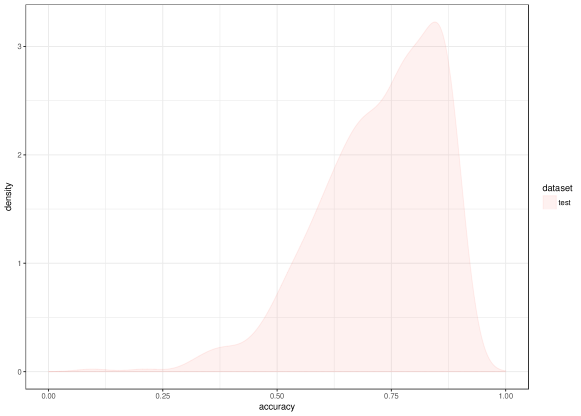
Figure 4: Posterior distribution of the classification accuracy. $n=500,\lambda=10^{-4}$.

4 Discussion

Weighted Bayesian Bootstrap (WBB) provides a computationally attractive solution to scalable Bayesian inference (Minsker et al. (2014); Welling and Teh (2011)) whilst accounting for parameter uncertainty by drawing samples from a weighted posterior distribution. WBB can also be used in conjunction with proximal methods (Parikh and Boyd (2013), Polson et al. (2015)) to provide sparsity in high dimensional statistica problems. With a similar ease of computation, WBB provides an alternative to ABC methods (Beaumont et al. (2009)) and Variational Bayes (VB) methods. A fruitful area for future research is the comparison of approximate Bayesian computation with simulated Bayesian Bootstrap inference.

Appendix A Stochastic Gradient Descent (SGD)

Stochastic gradient descent (SGD) method or its variation is typically used to find the deep learning model weights by minimizing the penalized loss function, $\sum_{i=1}^{n}w_{i}l_{i}(y_{i};\theta)+\lambda w_{p}\phi(\theta)$. The method minimizes the function by taking a negative step along an estimate $g^{k}$ of the gradient $\nabla\left[\sum_{i=1}^{n}w_{i}l_{i}(y_{i};\theta^{k})+\lambda w_{p}\phi(\theta^{k})\right]$ at iteration $k$. The approximate gradient is estimated by calculating

$$g^{k}=\frac{n}{b_{k}}\sum_{i\in E_{k}}w_{i}\nabla l_{i}(y_{i};\theta^{k})+\lambda w_{p}\frac{n}{b_{k}}\nabla\phi(\theta^{k})$$

Where $E_{k}\subset\{1,\ldots,n\}$ and $b_{k}=|E_{k}|$ is the number of elements in $E_{k}$. When $b_{k}>1$ the algorithm is called batch SGD and simply SGD otherwise. A usual strategy to choose subset $E$ is to go cyclically and pick consecutive elements of $\{1,\ldots,T\}$, $E_{k+1}=[E_{k}\mod n]+1$. The approximated direction $g^{k}$ is calculated using a chain rule (aka back-propagation) for deep learning. It is an unbiased estimator. Thus, at each iteration, the SGD updates the solution

$$\theta^{k+1}=\theta^{k}-t_{k}g^{k}$$

For deep learning applications the step size $t_{k}$ (a.k.a learning rate) is usually kept constant or some simple step size reduction strategy is used, $t_{k}=a\exp(-kt)$. Appropriate learning rates or the hyperparameters of reduction schedule are usually found empirically from numerical experiments and observations of the loss function progression.

References

- Beaumont et al. (2009) Beaumont, M. A., J.-M. Cornuet, J.-M. Marin, and C. P. Robert (2009). Adaptive approximate bayesian computation. Biometrika 96(4), 983–990.
- Bertail and Lo (1991) Bertail, P. and A. Y. Lo (1991). On johnson’s asymptotic expansion for a posterior distribution. Centre de Recherche en Economie et Statistique.
- Daniels and Young (1991) Daniels, H. and G. Young (1991). Saddlepoint approximation for the studentized mean, with an application to the bootstrap. Biometrika 78(1), 169–179.
- Efron (1981) Efron, B. (1981). Nonparametric standard errors and confidence intervals. Canadian Journal of Statistics 9(2), 139–158.
- Efron (2012) Efron, B. (2012). Bayesian inference and the parametric bootstrap. The Annals of Applied Statistics 6(4), 1971.
- Gelman and Meng (1998) Gelman, A. and X.-L. Meng (1998). Simulating normalizing constants: From importance sampling to bridge sampling to path sampling. Statistical Science, 163–185.
- Gordon et al. (1993) Gordon, N. J., D. J. Salmond, and A. F. Smith (1993). Novel approach to nonlinear/non-gaussian Bayesian state estimation. In IEE Proceedings F-Radar and Signal Processing, Volume 140, pp. 107–113. IET.
- Gramacy and Polson (2012) Gramacy, R. B. and N. G. Polson (2012). Simulation-based regularized logistic regression. Bayesian Analysis 7(3), 567–590.
- Hans (2009) Hans, C. (2009). Bayesian lasso regression. Biometrika 96(4), 835–845.
- Johnson (1970) Johnson, R. A. (1970). Asymptotic expansions associated with posterior distributions. The annals of mathematical statistics 41(3), 851–864.
- Lopes et al. (2012) Lopes, H. F., N. G. Polson, and C. M. Carvalho (2012). Bayesian statistics with a smile: a resampling-sampling perspective. Brazilian Journal of Probability and Statistics, 358–371.
- Minsker et al. (2014) Minsker, S., S. Srivastava, L. Lin, and D. Dunson (2014). Scalable and robust bayesian inference via the median posterior. In International Conference on Machine Learning, pp. 1656–1664.
- Mitchell (1994) Mitchell, A. F. (1994). A note on posterior moments for a normal mean with double-exponential prior. Journal of the Royal Statistical Society. Series B (Methodological), 605–610.
- Newton (1991) Newton, M. A. (1991). The weighted likelihood bootstrap and an algorithm for prepivoting. Ph. D. thesis, Department of Statistics, University of Washington, Seattle.
- Newton and Raftery (1994) Newton, M. A. and A. E. Raftery (1994). Approximate Bayesian inference with the weighted likelihood bootstrap. Journal of the Royal Statistical Society. Series B (Methodological), 3–48.
- Parikh and Boyd (2013) Parikh, N. and S. Boyd (2013). Proximal algorithms, in foundations and trends in optimization.
- Polson and Scott (2015) Polson, N. G. and J. G. Scott (2015). Mixtures, envelopes and hierarchical duality. Journal of the Royal Statistical Society: Series B (Statistical Methodology).
- Polson et al. (2015) Polson, N. G., J. G. Scott, and B. T. Willard (2015). Proximal algorithms in statistics and machine learning. Statistical Science 30(4), 559–581.
- Polson et al. (2014) Polson, N. G., J. G. Scott, and J. Windle (2014). The Bayesian bridge. Journal of the Royal Statistical Society: Series B (Statistical Methodology) 76(4), 713–733.
- Polson and Sokolov (2017) Polson, N. G. and V. Sokolov (2017). Deep learning: A bayesian perspective. Bayesian Analysis 12(4), 1275–1304.
- Rubin (1981) Rubin, D. B. (1981). The Bayesian bootstrap. The Annals of Statistics 9(1), 130–134.
- Strawderman et al. (2013) Strawderman, R. L., M. T. Wells, and E. D. Schifano (2013). Hierarchical bayes, maximum a posteriori estimators, and minimax concave penalized likelihood estimation. Electronic Journal of Statistics 7, 973–990.
- Taddy et al. (2015) Taddy, M., C.-S. Chen, J. Yu, and M. Wyle (2015). Bayesian and empirical bayesian forests. arXiv preprint arXiv:1502.02312.
- Tibshirani (2014) Tibshirani, R. J. (2014). Adaptive piecewise polynomial estimation via trend filtering. The Annals of Statistics 42(1), 285–323.
- Van Der Pas et al. (2014) Van Der Pas, S., B. Kleijn, and A. Van Der Vaart (2014). The horseshoe estimator: Posterior concentration around nearly black vectors. Electronic Journal of Statistics 8(2), 2585–2618.
- Welling and Teh (2011) Welling, M. and Y. W. Teh (2011). Bayesian learning via stochastic gradient langevin dynamics. In Proceedings of the 28th International Conference on Machine Learning (ICML-11), pp. 681–688.
- West (1992) West, M. (1992). Modelling with Mixtures. In Bayesian Statistics 4, 503–524.