Constraints on light Dark Matter fermions from relic density consideration and Tsallis statistics

Abstract

The cold dark matter fermions with mass MeV scale, pair produced inside the supernova SN1987A core, can freely stream away from the supernovae and hence contributes to its energy loss rate. Similar type of DM fermions(having similar kind of coupling to the standard model photon), produced from some other sources earlier, could have contributed to the relic density of the Universe. Working in a theory with an effective dark matter-photon coupling (inversely proportional to the scale $\Lambda$) in the formalism of Tsallis statistics, we find the dark matter contribution to the relic density and obtain a upper bound on $\Lambda$ using the experimental bound on the relic density for cold non-baryonic matter i.e. $\Omega h^{2}=0.1186\pm 0.0020$. The upper bound obtained from the relic density is shown with the lower bound obtained from the Raffelt’s criterion on the emissibity rate of the supernovae SN1987A energy loss $\dot{\varepsilon}(e^{+}e^{-}\rightarrow\chi\overline{\chi})\leq 10^{19}~{}\rm{erg~{}g^{-1}s^{-1}}$ and the optical depth criteria on the free streaming of the dark matter fermion (produced inside the supernovae core). As the deformation parameter $q$ changes from $1.0$ (undeformed scenario) to $1.1$(deformed scenario), the relic density bound on $\Lambda$ is found to vary from $\sim 4.9\times 10^{7}$ TeV to $1.6\times 10^{8}$ TeV for a fermion dark matter($\chi$) of mass $m_{\chi}=30~{}\rm{MeV}$, which is almost $10$ times more than the lower bound obtained from the SN1987A energy loss rate and the optical depth criteria.

Keywords: Dark matter, Relic density, Supernova cooling, Tsallis statistics, free-streaming,

1 Introduction

Experimental evidences from DAMA-LIBRA, CRESST, SuperCDMS, LUX, PICO are strengthening the concept of dark matter(DM) day by day. It is now well established that dark matter is essential to build the large-scale structure of our Uniniverse. At galactic and sub-galactic scales, there are evidences for the structure formation. These includes galactic rotation curves, the weak gravitational lensing of distant galaxies by foreground structures. In 1932 the Dutch astronomer Jan Hendrik Oort analyzed the acceleration of matter by studying the vertical motions of all known stars near the Galactic plane, which can be thought as the first indication of some unseen mass. After estimating the gravitational potential for the luminous matter Oort surprisingly found out that the potential necessary to keep the known stars bound to the Galactic disk is simply not sufficientMRoos:2010wb ; MRoos:2012cc . The second possible indication (historically) for the possible presence of dark matter at a cosmological distance scale in our galaxy, was found in 1933 by Fritz Zwicky Zwicky . Zwicky measured the radial velocities of member galaxies in the Coma cluster and the cluster radius. Using the virial theorem Zwicky made an estimate of the average mass of the galaxies within the cluster and found that it is 160 times larger than expected from their luminosity and from this he proposed that the missing matter was dark. He found that the orbital velocities of member galaxies in the Coma cluster were almost a factor of ten larger than expected from the summed mass of all galaxies belonging to the Coma cluster. A large amount of non-luminous matter, dubbed as dark matter, is required in order to hold galaxies together the cluster. Current data which constrain the energy densities of the Universe in normal matter (baryons), dark matter and dark energy $\Lambda$ to be $\sim 5\%$, $\sim 27\%$ and $\sim 68\%$, respectively. This means that the normal matter we know and that makes up all stars and galaxies only accounts for $5\%$ of the content of the universe! Dark matter, five times more than the normal luminous matter, accounts for a quarter of the Universe Feng .

Since the DM has no electric or magnetic charge, it does not interact electromagnetically with the normal luminous matter; even if it does so, the interaction is very weak. It does not absorb, reflect or emit light, making it extremely hard to detect. So far, researchers have been able to infer the existence of dark matter only from the gravitational effect it seems to have on visible matter.
But the nature of dark matter remains a mystery for a long time. A wide range of collider and astrophysical study suggests that it is a Weakly Interacting Massive Particle(WIMP) of mass ranging from a few MeV to few tens of GeV. Theories suggest that DM candidates are most likely to be found in the beyond the Standard Model(SM) physics e.g. in models with supersymmetry or extra dimension(s) etc. Direct detection of DM includes its interaction with nucleons in underground detectors, whereas indirect detection through DM annihilation to SM states (i.e. neutrinos) inside the Sun has been done. Experiments at the Large Hadron Collider(LHC) and the upcoming electron-positron linear collider(LC) will give more information about the dark matter as the missing energy signature. See JKG ; BHS ; Feng for a review on dark matter searches. Here we are to investigate the light dark matter fermions contribution to relic density. The concerned dark matter fermions may be pair produced in the crust of the supernovae core, which afterwords can freely stream away while taking away the energy released in supernovae explosion and also from some other sources like bullet cluster etc. In a work Guha et al.Atanu investigated the role of fermion dark matter in the supernovae SN1987A cooling: they worked in an effective DM model where the SM photon couples with the dark matter fermion through a magnetic/electric dipole moment operator. Working with the formalism of Tsallis statistics and applying the Raffelt’s criteria Raffelt on the supernovae energy loss rate and free streaming criteria, they found a lower bound on $\Lambda\sim 10^{6}-10^{7}$ TeV. The DM produced inside the supernovae crust may contribute to the relic density after they freely stream away from the supernovae. Here we are to investigate the DM relic density upper bound on $\Lambda$ and show those along with the lower bounds obtained from the SN1987A energy loss rate and free streaming criteria on DM fermions.
  The outline is as follows. In Sec. II, we give a brief description of the relic density calculation and introduce the Tsallis statistics (characterized by the deformation parameter $q$). In Sec. III, we discuss the contribution of similar type of DM fermions to the relic density, which is pair produced in electron-positron annihilation inside the SN1987A core. But they could have been produced from some other sources as well, only thing is that, they are similar in nature and they couple to the standard model photons in a similar way. We obtained their contribution to the relic density using the lower bound on $\Lambda$ obtained previously from SN cooling and free streaming Atanu . In that way this contribution signifies the minimum contribution of the concerned DM fermions. Because relic density contribution is directly proportional to the scale $\Lambda$. Also we can see the contribution is very less(almost $0.1\%-1\%$ of the total non-baryonic density, $0.1186$). This is because they are very light(low mass contribution) and if we consider the supernovae explosions as one of the major production process of those DM fermions, the explosion energy is not enough to produce them in significant amount. Consequently they can not significantly contribute to the dark matter relic density. But we can obtain a lower and upper bound on the effective scale $\Lambda$ from these two consideration(SN cooling and relic density). The numerical analysis part is presented in Sec. IV. Using the experimental value of the non-baryonic relic density i.e. $0.1186\pm 0.0020$ (obtained from the measurement of CMB(cosmic microwave background) anisotropy and the spatial distribution of galaxies), we obtain a upper bound on the scale $\Lambda$ of the dark matter effective theory in the deformed ($q>1$) and undeformed ($q=1$) scenarios, respectively. Using the Raffelt’s criteria and the optical depth criteria(based on free streaming of dark matter fermions), we obtained the lower bound on $\Lambda$ Atanu and in the present work we show them with the relic density bound obtained in Sec. IV. Finally, we summarize our results and conclude in Sec. V.

2 Boltzmann equation, Relic density calculation and $q$-deformed statistics

2.1 Relic density contribution and experimental estimation

The time evolution of the phase space distribution in plasma cosmology is described by Liouville equation, where we consider the dynamics of plasma(ionized gas) as a key element in describing the physics of the large-scale structure formation of the Universe kolb .

Liouville equation

$$\frac{d\rho}{dt}=\frac{\partial\rho}{\partial t}+\sum_{i=1}^{n}\left(\frac{\partial\rho}{\partial q_{i}}\dot{q_{i}}+\frac{\partial\rho}{\partial p_{i}}\dot{p_{i}}\right)$$ (1)

An era of the early stages of the Universe, when various particle candidates fall out of thermal equilibrium with each other, is popularly known as freeze-out. Rapid expansion of the Universe at that time is mainly responsible for this which causes the interaction rate of those particle to decrease. As a result they don’t interact to each other further and tend to contribute to the cosmic abundances as a form of mass of radiation. After freeze-out(decoupling) the microscopic evolution of the phase space distribution of a particle species is described by Boltzmann equation kolb ; gondolo

$$L[f]=C[f]$$ (2)

where, $L$ is the Liouville operator and $C$ stands for the collision operator which represents the number of concerned particles per unit phase-space volume those are lost or gained per unit time under collision with other particles.

Relativistic generalized form of the Liouville operator becomes

$$\hat{L}=p^{\alpha}\frac{\partial}{\partial x^{\alpha}}-\Gamma^{\alpha}_{\beta\gamma}p^{\beta}p^{\gamma}\frac{\partial}{\partial p^{\alpha}}$$ (3)

For spatially homogeneous and isotropic phase-space density the Liouville operator in the Friedmann-Robertson-Walker cosmological model is given by

$$L[f]=\frac{\partial f}{\partial t}-H\frac{\mid p\mid^{2}}{E}\frac{\partial f}{\partial E}$$ (4)

Therefore the Boltzmann equation in FRW cosmology becomes

$$\frac{dn}{dt}+3Hn=\frac{g}{(2\pi)^{3}}\int\hat{C}[f]\frac{d^{3}p}{E}$$ (5)

where, the number density of the particle in terms of phase space density is given by

$$n(t)=\frac{g}{(2\pi)^{3}}\int d^{3}pf(E,t)$$ (6)

and $g$ stands for the degree of freedom.

Defining two new variables $Y=\frac{n}{s},~{}x=\frac{m}{T}$($s,m,T$ denotes the entropy density, mass of the particle species and temperature respectively) and writing down the collision term for a particular process we get the Boltzmann equation as follows kolb ; gondolo ; majumdar

$$\frac{dY}{dx}=\frac{1}{3H}\frac{ds}{dx}<\sigma v_{rel}>\left(Y^{2}-Y^{2}_{eq}\right)$$ (7)

with the thermal averaged crosssection times relative velocity

$$<\sigma v_{rel}>=\frac{\int\sigma v_{rel}e^{-E_{1}/T}e^{-E_{2}/T}d^{3}p_{1}d^{3}p_{2}}{\int e^{-E_{1}/T}e^{-E_{2}/T}d^{3}p_{1}d^{3}p_{2}}$$ (8)

Working in the standard FRW cosmology

$$H=\left(\frac{8}{3}\pi G\rho\right)^{\frac{1}{2}}$$ (9)

we can substitute the following expressions for the density $\rho$ and entropy density $s$ in Eq.(8)

$$\rho=g_{eff}(T)\frac{\pi^{2}}{30}T^{4}$$

$$s=h_{eff}(T)\frac{2\pi^{2}}{45}T^{3}$$ (10)

and subsequently we get the following form of the Boltzmann equation gondolo ; majumdar

$$\frac{dY}{dx}=-\left(\frac{45}{\pi}G\right)^{-\frac{1}{2}}\frac{m}{x^{2}}g_{*}^{\frac{1}{2}}<\sigma v>\left(Y^{2}-Y^{2}_{eq}\right)$$ (11)

where,

$$g_{*}^{\frac{1}{2}}=\frac{h_{eff}}{g_{eff}^{\frac{1}{2}}}\left(1+\frac{1}{3}\frac{T}{h_{eff}}\frac{dh_{eff}}{dT}\right)$$ (12)

with the total effective degree of freedom for all final species $g_{eff}(T)=\sum_{i}g_{i}(T)$ and $h_{eff}(T)=\sum_{i}h_{i}(T)$. The effective degrees of freedom for each species are given by gondolo

$$g_{i}(T)=\frac{15g_{i}}{\pi^{4}}x_{i}^{4}\int_{1}^{\infty}\frac{z\sqrt{z^{2}-1}}{\exp(x_{i}z)+\eta_{i}}zdz$$

$$h_{i}(T)=\frac{45g_{i}}{4\pi^{4}}x_{i}^{4}\int_{1}^{\infty}\frac{z\sqrt{z^{2}-1}}{\exp(x_{i}z)+\eta_{i}}\frac{4z^{2}-1}{3z}dz$$ (13)

with $x_{i}=m_{i}/T$, where, $m_{i}$ stands for the mass of that particular species and $\eta_{i}=1$ for Fermi-Dirac statistics and $\eta_{i}=-1$ for Bose-Einstein statistics.

After decoupling(freezing-out) we can neglect the term $Y_{eq}$ majumdar and integrating from the freeze-out period to the present epoch we get

$$\frac{1}{Y_{0}}=\left(\frac{45}{\pi}G\right)^{-\frac{1}{2}}\int_{T_{0}}^{T_{f}}g_{*}^{\frac{1}{2}}<\sigma v>dT$$ (14)

Again the value of $\frac{1}{Y}$ at $T=T_{f}$ has been neglected as at freeze-out the number density of the concerned particle is considered to be very high which results the term $\frac{1}{Y_{f}}=\frac{s_{f}}{n_{f}}$ to be very small compared to the other terms.

Relic density of the concerned particle at present can easily be obtained after evaluating $Y_{0}$ in the units of the critical density as follows edsjo ; gelmini

$$\Omega_{\chi}=\frac{\rho^{0}_{\chi}}{\rho_{crit}}=\frac{m_{\chi}s_{0}Y_{0}}{\rho_{crit}}$$ (15)

with the critical density $\rho_{crit}=\frac{3H^{2}}{8\pi G}$, $s_{0}$ in the entropy density today. With the knowledge of the present day background radiation temperature $T_{0}=2.726~{}\rm{K}=2.35\times 10^{-16}~{}\rm{TeV}$ we obtain

$$\Omega_{\chi}h^{2}=2.755\times 10^{11}~{}m_{\chi}~{}Y_{0}$$ (16)

Where the value of $m_{\chi}$ is in TeV. The experimental value of the non-baryonic relic density i.e., $0.1186\pm 0.0020$, has been obtained from the measurement of CMB(cosmic microwave background) anisotropy and the spatial distribution of galaxies (PDG 2017).

2.2 Fluctuating temperature and Tsallis statistics

$\chi^{2}$ distribution takes the following form in the $q$-deformed statistics Beck_cohen to account for the temperature ($T$) fluctuations Kaniadakis

$$f(\beta)=\frac{1}{\Gamma\left(\frac{n}{2}\right)}\left(\frac{n}{2\beta_{0}}\right)^{n/2}\beta^{\frac{n}{2}-1}~{}\exp\left(-\frac{n\beta}{2\beta_{0}}\right)$$ (17)

where $n$ is the degree of the distribution and $\beta={1\over{kT}}$. The average of the fluctuating inverse temperature $\beta$ can be estimated as

$$\langle\beta\rangle=n\langle X_{i}^{2}\rangle=\int_{0}^{\infty}\beta f(\beta)d\beta=\beta_{0}$$ (18)

Taking into account the local temperature fluctuation, integrating over all $\beta$, we find the $q$-generalized relativistic( with particle energy $E=\sqrt{{\bf p}^{2}c^{2}+m^{2}c^{4}}$) Maxwell-Boltzmann distribution

$${\mathcal{P}}(E)\sim\frac{E^{2}}{\left(1+b(q-1)E\right)^{\frac{1}{q-1}}}$$ (19)

where $q=1+\frac{2}{n+6}$ and $b=\frac{\beta_{0}}{4-3q}$. Its generalization to Fermi-Dirac and Bose-Einstein distribution is worked out in Beck_super . The average occupation number of any particle within this $q$-deformed statistics ( Tsallis statistics Tsallis ) formalism is given by $f_{i}(\beta,E_{i})$ ($i=1,2$ corresponds to particles) where

$$f_{i}(\beta,E_{i})=\frac{1}{\left(1+(q-1)bE_{i}\right)^{\frac{1}{q-1}}\pm 1}$$ (20)

where the $-$ sign is for bosons and the $+$ sign is for fermions. Note that the effective Boltzmann factor $x_{i}=\left(1+(q-1)bE_{i}\right)^{-\frac{1}{q-1}}$ approaches to the ordinary Boltzmann factor $e^{-bE_{i}}(=e^{-\beta_{0}E_{i}})$ as $q\rightarrow 1$. For more discussion related to this and to find its various applications please refer to Atanu ; Atanu3 ; Atanu4 ; Tsallis_book ; Sumiyoshi_book ; Beck_cosmic ; Bediaga-ep ; Beck-ep ; Beck_deform ; Beck_dark .

2.3 Brief discussion on SN1987A cooling and Free streaming of produced DM particles

2.3.1 SN1987A cooling

The supernova SN1987A was the most evident example of a core-collapse type II supernova explosion till date, which was even visible to the naked eye. After four days of the SN1987A (or AAVSO 0534-69) explosion in the Large Magellanic Cloud (a dwarf galaxy satellite of the Milky Way), a blue supergiant massive star was disappeared. Thus the progenitor of SN1987A was identified as Sanduleak ($M\sim 20\,M_{\odot}$), a B3 supergiant in the constellation Dorado at a distance approximately $51.4$ kiloparsecs ($1.68\times 10^{5}$ light-years) from Earth. An enormous amount of energy was released in the SN1987A explosion which equals to the gravitational binding energy $E_{g}$ of the proto-neutron star (of mass $M_{PNS}$) which is given by

$$E_{g}=\frac{3G_{N}M_{PNS}^{2}}{5R_{NS}}\sim 3.0\times 10^{53}\;{\rm erg.}$$ (21)

Here $M_{PNS}=1.5M_{\odot}$, $R_{NS}=10~{}{\rm Km}$ and $G_{N}$ is the Newton’s gravitational constant. As per present understanding, neutrinos carry away $99\%$ of the huge amount of released energy and the remaining $1\%$ contributes to the kinetic energy of the explosion. For the earth based detectors the primary astrophysical interest was to detect this neutrino burst. This neutrino flux was first detected by the two collaborations Kamiokande Kamioka and IMBIMB using their earth based detectors. The data obtained by them suggest that, in a couple of seconds about $10^{53}~{}\rm{ergs}$ energy was released in the SN1987A explosion. The observed neutrino luminosity in the detector(IMB or Kamiokande) is $L_{\nu}\sim 3\times 10^{53}\;{\rm erg~{}s^{-1}}$ (including $3$ generations of neutrinos and anti-neutrinos i.e. $\nu_{e},~{}\nu_{\mu},~{}\nu_{\tau}$ and ${\overline{\nu_{e}}},~{}{\overline{\nu_{\mu}}},~{}{\overline{\nu_{\tau}}}$). So $\tilde{L}_{\nu}=\frac{L_{\nu}}{6}\sim 3\times 10^{52}~{}{\rm erg~{}s^{-1}}$. The mass of a typical proto-neutron star $M_{PNS}=1.5M_{\odot}=3\times 10^{33}~{}{\rm g}$. So, the average energy loss per unit mass is $\frac{\tilde{L}_{\nu}}{M_{PNS}}\simeq 1\times 10^{19}~{}{\rm erg~{}g^{-1}s^{-1}}$. Note that this is the energy carried away by each of the above 6 (anti)-neutrino species.

For any new physics channel, Raffelt’s criteria states that, besides neutrino, if Kaluza-Klein graviton, Kaluza-Klein radion, axion also take away energy, the energy-loss rate due to these new channels $\epsilon_{new}$ should be less than the above average energy loss rate Raffelt , i.e.

$$\epsilon_{new}\leq 10^{19}~{}\rm{erg~{}g^{-1}~{}s^{-1}}$$ (22)

and this follows from the observed neutrino luminosity per species (total six neutrinos and anti-neutrinos, three types each). If any energy-loss mechanism has an emissivity greater than $10^{19}~{}\rm{erg~{}g^{-1}~{}s^{-1}}$, then it will remove sufficient energy from the explosion to invalidate the current understanding of core-collapse supernova.

Using the Raffelt’s criteria of the supernova energy loss rate for any new physics channel, we constrained the scale $\Lambda$ of the dark matter effective theory Atanu . Now in a realistic scenario, since the core temperature of the supernova is fluctuating, we worked within the formalism of Tsallis statisticsTsallis ; Atanu ; Atanu3 ; Atanu4 where this temperature fluctuation is taken into account.

2.3.2 Free streaming of produced dark matter fermions from SN1987A

Now the constraint on the effective scale $\Lambda$ of the dark matter effective theory obtained using the Raffelt’s criteria holds to be truly sensible if the produced dark matter fermion free streams out of the supernova without getting trapped. In order to find the free streaming/trapping their mean free path is to be evaluated Dreiner , which is given by

$$\lambda_{\chi}=\frac{1}{n_{e}\cdot\sigma_{e\chi\rightarrow e\chi}}$$ (23)

where $n_{e}(=8.7\times 10^{43}~{}\rm{m^{-3}})$ is the number density of the colliding electrons in the supernova and $\sigma_{e\chi\rightarrow e\chi}$ is the cross section for the scattering of the dark matter fermion on the electron which is related via the crossing symmetry to the annihilation cross section $\sigma_{ee\rightarrow\chi\chi}$. Now, most of the dark matter particles produced in the outermost $10\%$ of the star ($0.9R_{c}<r<R_{c}$) from electron-positron annihilation DHLP ; Atanu . Then any of the dark matter particles produced in electron-positron annihilation while propagating through the proto-neutron star, can undergo scattering due to the presence of neutrons and electrons inside the star. In the case of supernova cooling, neutron-dark matter particle scattering will be negligible for free streaming due to neutron mass Dreiner ; Atanu . We use the optical depth criteria Dreiner

$$\int_{r_{0}}^{R_{c}}\frac{dr}{\lambda_{\chi}}\leq\frac{2}{3}$$ (24)

to investigate whether the dark matter fermion produced at a depth $r_{0}$ free streams out of the supernova and takes away the released energy or gets trapped inside the supernova. Here we set $r_{0}=0.9R_{c}$ in our analysis, where $R_{c}$ ($\simeq 10$ km) is the radius of the supernova core (proto-neutron star) Dreiner ; Atanu . From the optical depth criteria, we find that minimum length of the mean free path for free streaming $\lambda_{fs}$ is $\lambda^{\rm{min}}_{fs}=1.5~{}\rm{km}$ and it increases with $\Lambda$. On the other hand we can get a lower bound on the effective scale $\Lambda$ using the optical depth criterion which has been done in the numerical section and also in Atanu .

3 Light fermionic Dark matter contribution to the relic density

Electrons are abundant in supernovae. The dark matter fermions may be pair produced in the $s$-channel annihilation of electron and positron [Fig. 1(a)]: $e^{-}(p_{1})e^{+}(p_{2})\stackrel{{\scriptstyle\gamma}}{{\longrightarrow}}\chi(p_{3})\bar{\chi}(p_{4})$.

((a))

((b))

Figure 1: Feynman diagram for the processes $e^{-}e^{+}\stackrel{{\scriptstyle\gamma}}{{\longrightarrow}}\chi\bar{\chi}$ and $\chi\bar{\chi}\stackrel{{\scriptstyle\gamma}}{{\longrightarrow}}e^{-}e^{+}$.

To estimate the contribution to the relic density of the produced dark matter fermion, we have to look for the reverse process [Fig. 1(b)] $\chi\bar{\chi}\stackrel{{\scriptstyle\gamma}}{{\longrightarrow}}e^{-}e^{+}$.

The effective Lagrangian of describing photon($\gamma$) and dark matter fermion ($\chi$) interaction is given by

$$\mathcal{L}=-\frac{i}{2}\bar{\chi}\sigma_{\mu\nu}(\mu_{\chi}+\gamma_{5}d_{\chi})\chi F^{\mu\nu}$$ (25)

where $F^{\mu\nu}=\partial^{\mu}A^{\nu}-\partial^{\nu}A^{\mu}$, the electromagnetic field strength tensor. Here $\mu_{\chi}$ and $d_{\chi}$ correspond to the magnetic dipole moment and the electric dipole moment of the dark matter fermion $\chi$. $\sigma^{\mu\nu}=\frac{i}{2}[\gamma^{\mu},\gamma^{\nu}]$ is the spin tensor. The $4$-momentum vectors of the initial and final state particles (Fig. 1(b)) in the center-of-mass frame are given by

$$p_{1} = \left(E,0,0,p_{z}\right);~{}p_{2}=\left(E,0,0,-p_{z}\right);$$

$$p_{3} = \left(E^{\prime},p\sin\theta\cos\phi,p\sin\theta\sin\phi,p\cos\theta\right);$$

$$p_{4} = \left(E^{\prime},-p\sin\theta\cos\phi,-p\sin\theta\sin\phi,-p\cos\theta\right).$$

The spin-averaged amplitude square for the process $\chi(p_{1})\bar{\chi}(p_{2})\stackrel{{\scriptstyle\gamma}}{{\longrightarrow}}e^{-}(p_{3})e^{+}(p_{4})$ is given by

$$\overline{|\mathcal{M}|^{2}}=4\pi\alpha[\mu_{\chi}^{2}\left\{s(1-\cos^{2}\theta)+4m_{\chi}^{2}(1+\cos^{2}\theta)\right\}+d_{\chi}^{2}\left\{(s-4m_{\chi}^{2})(1-\cos^{2}\theta)\right\}]$$ (26)

The differential cross section for the process is

$$\frac{d\sigma}{d\Omega}({\chi\bar{\chi}\stackrel{{\scriptstyle\gamma}}{{\longrightarrow}}e^{-}e^{+}})=\frac{1}{64\pi^{2}s}\cdot\left(\sqrt{1-\frac{4m_{\chi}^{2}}{s}}\right)^{-1}\cdot\overline{|\mathcal{M}|^{2}}$$ (27)

Finally, the total cross section is given by

$$\sigma({\chi\bar{\chi}\stackrel{{\scriptstyle\gamma}}{{\longrightarrow}}e^{-}e^{+}})=\frac{\alpha}{6s}\cdot\left(\sqrt{1-\frac{4m_{\chi}^{2}}{s}}\right)^{-1}\cdot\left[\mu_{\chi}^{2}(s+8m_{\chi}^{2})+d_{\chi}^{2}(s-4m_{\chi}^{2})\right]$$ (28)

Here $m_{\chi}$ is the dark matter mass, $\alpha=\frac{e^{2}}{4\pi}$ and $s=(p_{1}+p_{2})^{2}=(p_{3}+p_{4})^{2}$ is the Mandelstam variable.

Thermal averaged cross-section times velocity

The thermal averaged cross-section times velocity for the dark matter fermion pair annihilation is given by kolb ; gondolo

$$<\sigma_{\chi\overline{\chi}\rightarrow e^{-}e^{+}}~{}V_{rel}>=\frac{\int_{m_{\chi}}^{\infty}\int_{m_{\chi}}^{\infty}dE_{1}~{}dE_{2}~{}\sqrt{E_{1}^{2}-m_{\chi}^{2}}~{}\sqrt{E_{2}^{2}-m_{\chi}^{2}}~{}(E_{1}+E_{2})^{2}~{}\sigma_{\chi\overline{\chi}\rightarrow e^{-}e^{+}}~{}f_{1}~{}f_{2}}{\int_{m_{\chi}}^{\infty}\int_{m_{\chi}}^{\infty}dE_{1}~{}dE_{2}~{}E_{1}~{}E_{2}~{}\sqrt{E_{1}^{2}-m_{\chi}^{2}}~{}\sqrt{E_{2}^{2}-m_{\chi}^{2}}~{}f_{1}~{}f_{2}}$$

where the c.m. energy $E_{c.m.}(=E_{1}+E_{2})=2E$ (where $E_{1}=E_{2}=E$) and the relative velocity $V_{rel}=\frac{s}{4E_{1}E_{2}}$. The cross section $\sigma_{\chi\overline{\chi}\rightarrow e^{-}e^{+}}$ is given in Eq. (28) and $f_{i}=1/D_{i}$ where $D_{i}=\left(1+\frac{b}{\tau}E_{i}\right)^{\tau}+1$ with $\rm{i}=1,2$. Here $b=\frac{\beta_{0}}{4-3q}$, $\beta_{0}=\frac{1}{k_{B}T}$ (we are working in the unit where $k_{B}=1$) and $\tau={1\over q-1}$. The DM fermion particle and antiparticle number densities $n_{\chi}=\int\frac{2d^{3}p_{1}}{(2\pi)^{3}}~{}{D_{1}}^{-1}$ and $n_{\bar{\chi}}=\int\frac{2d^{3}p_{2}}{(2\pi)^{3}}~{}{D_{2}}^{-1}$. Introducing the dimensionless variables $x_{i}=E_{i}/T$ ($i=1,2$), we can finally write the Eq. (3) as

$$<\sigma_{\chi\overline{\chi}\rightarrow e^{-}e^{+}}~{}V_{rel}>=\frac{\alpha}{6}\frac{\int_{\frac{m_{\chi}}{T}}^{\infty}\int_{\frac{m_{\chi}}{T}}^{\infty}dx_{1}~{}dx_{2}~{}\sqrt{x_{1}^{2}-\frac{m_{\chi}^{2}}{T^{2}}}~{}\sqrt{x_{2}^{2}-\frac{m_{\chi}^{2}}{T^{2}}}~{}{\mathcal{F}}~{}f_{1}~{}f_{2}}{\int_{\frac{m_{\chi}}{T}}^{\infty}\int_{\frac{m_{\chi}}{T}}^{\infty}dx_{1}~{}dx_{2}~{}x_{1}~{}x_{2}~{}\sqrt{x_{1}^{2}-\frac{m_{\chi}^{2}}{T^{2}}}~{}\sqrt{x_{2}^{2}-\frac{m_{\chi}^{2}}{T^{2}}}~{}f_{1}~{}f_{2}}$$ (30)

where the function $\mathcal{F}$ is given by

$${\mathcal{F}}=\left(\sqrt{1-\frac{4m_{\chi}^{2}}{T^{2}(x_{1}+x_{2})^{2}}}\right)^{-1}\cdot\left[\mu_{\chi}^{2}\left\{(x_{1}+x_{2})^{2}+\frac{8m_{\chi}^{2}}{T^{2}}\right\}+d_{\chi}^{2}\left\{(x_{1}+x_{2})^{2}-\frac{4m_{\chi}^{2}}{T^{2}}\right\}\right]$$

Noting the fact that in the $q\rightarrow 1$ limit, the $q$-deformed distribution formula gets converted to either the Bose-Einstein or Fermi-Dirac statistical distribution formula (which describes the undeformed scenario) (see the Appendix for a proof), i.e.

$$f_{i}(\beta,E_{i})=\frac{1}{\left(1+(q-1)bE_{i}\right)^{\frac{1}{q-1}}\pm 1}~{}\stackrel{{\scriptstyle q\rightarrow 1}}{{\longrightarrow}}\frac{1}{e^{bE_{i}}\pm 1}\left(=\frac{1}{e^{\beta_{0}E_{i}}\pm 1}\right)$$ (32)

where $e^{bE_{i}}=e^{\beta_{0}E_{i}}$ with $b=\frac{\beta_{0}}{4-3q}=\beta_{0}$ for $q\rightarrow 1$ and $\beta_{0}$ is the inverse equilibrium temperature. Now using Eq.(14) we can evaluate $Y_{0}$ and consequently the relic density for the pair of DM fermions using Eq.(16).

4 Numerical Analysis

The dark matter produced inside the supernova core via the channel $e^{-}e^{+}\rightarrow\chi\overline{\chi}$ [Fig. 1(a)] can contribute to the supernova energy loss rate and also similar type of DM fermions(does not depend on the source of production, maybe produced much earlier from other sources as well) contribute to the relic density via the process $\chi\overline{\chi}\rightarrow e^{-}e^{+}$ [Fig. 1(b)]. Since the core temperature(T) of the supernova is fluctuating, we follow the $\chi^{2}$ distribution analysis technique Beck_cohen here, where the temperature distribution is characterized by its mean value $T(=T_{SN})=30~{}\rm{MeV}$ (see Sec. II B for more details about $\chi^{2}$ distribution). As mentioned earlier, due to the temperature fluctuation, the ensemble of nucleons, electrons, dark matter fermions, photons inside the supernova will tend to follow $q$-deformed or Tsallis statistics Tsallis (when the deformation parameter $q\neq 1$) which is different from the usual Fermi-Dirac and Bose-Einstein statistics (when $q=1$). We investigate here the sensitivity of $q$ on the dark matter effective scale $\Lambda$ for a dark matter fermion of mass($m_{\chi}$) varying between $1\mbox{-}100~{}\rm{MeV}$.

4.1 Bound on the effective scale $\Lambda$ from the relic density of DM fermions obtained from $\chi\overline{\chi}\stackrel{{\scriptstyle\gamma}}{{\longrightarrow}}e^{+}+e^{-}$ process

Depending on whether the effective coupling of dark matter fermion with photon is characterized by a dipole moment operator of magnetic or electric type, there can be three cases as mentioned below Atanu :

1. Case I: $\mu_{\chi}(\sim 1/\Lambda_{\mu})\neq 0,~{}d_{\chi}(\sim 1/\Lambda_{d})=0$.

2. Case II: $\mu_{\chi}(\sim 1/\Lambda_{\mu})=0,~{}d_{\chi}(\sim 1/\Lambda_{d})\neq 0$.

3. Case III: $\mu_{\chi}(\sim 1/\Lambda_{\mu})\neq 0,~{}d_{\chi}(\sim 1/\Lambda_{d})\neq 0$. Here $\Lambda_{\mu}=\Lambda_{d}=\Lambda$.

Here $\Lambda$ is the scale of the dark matter effective theory. In each of the above three cases, we have two possible scenarios corresponding to $q\neq 1$ (deformed scenario) and $q=1$ (undeformed scenario).
We next calculate the dark matter contribution to the relic density $\Omega h^{2}$. We obtained consistent results as the contribution is much less than $0.1186$. In Fig. 2, we have plotted $\Omega h^{2}$ as a function of the dark matter mass $m_{\chi}$ for different $q$ values corresponding to $\Lambda$. The horizontal line corresponds to the current experimental bound on the non-baryonic dark matter relic density $\Omega h^{2}=0.1186\pm 0.0020$ (PDG 2017) and the lower set of curves corresponding to different $\Lambda$ values (lower bound obtained from the SN1987A cooling Atanu ) and $q=1,~{}1.05$ and $1.1$, respectively.

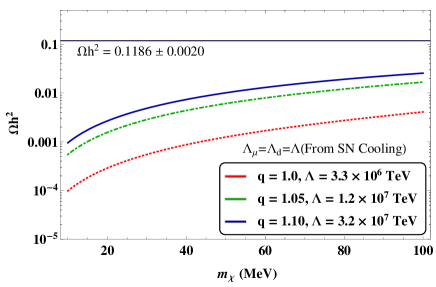
Figure 2: $\Omega h^{2}$ are plotted against $m_{\chi}$ (in MeV) for $q=1,1.05~{}\rm{and}1.1$ for the value of $\Lambda$($\Lambda_{\mu}=\Lambda_{d}=\Lambda$, Case III) obtained using Raffelt’s criteria Atanu .

We see that relic density for contribution of a DM fermion of mass $30$ MeV from $5\times 10^{-4}$ to $5\times 10^{-3}$ as the deformation parameter $q$ varies from $1.0$ to $1.1$. For a given deformation i.e. $q=1.1$, $\Omega h^{2}$ varies from $0.001$ to $0.02$ as $m_{\chi}$ increases from $10$ to $100~{}\rm{MeV}$. This is as per the expectation because massive DM fermions should contribute more to the relic density in principle.

In Fig. 3, we have plotted the upper bound $\Lambda$ as a function of $m_{\chi}$ for $q=1$(Fig. 3(a)) and $q=1.1$(Fig. 3(b)) corresponding to $\Omega h^{2}=0.1186$ for three cases.

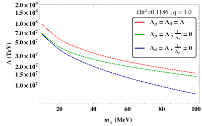
((a))

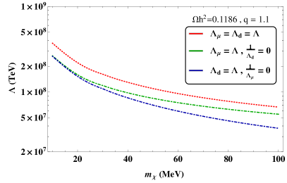
((b))

Figure 3: $\Lambda$ (in TeV) is plotted against $m_{\chi}$ (in MeV) for $q=1~{}\rm{and}~{}q=1.1$.

For a given $q$, the upper bound on $\Lambda$ decreases as $m_{\chi}$ increases. As an example, for $q=1.0$, we see that as $m_{\chi}$ increases from $10$ to $100~{}\rm{MeV}$, $\Lambda$(Case III) decreases from $1\times 10^{8}~{}\rm{TeV}$ to $1.6\times 10^{7}~{}\rm{TeV}$. On the right, the same is shown for $q=1.1$, where $\Lambda$ changes from $\sim 4\times 10^{8}~{}\rm{TeV}$ to $\sim 7\times 10^{7}~{}\rm{TeV}$ for the same $m_{\chi}$ range. In Fig. 4 we have plotted the upper bound on $\Lambda$ (obtained from the relic density constraint) as a function of $q$ corresponding to $m_{\chi}=10(\rm{topmost}),~{}30~{}(\rm{middle})$ and $50~{}(\rm{lowermost})$ MeV (for Case III) using $\Omega h^{2}=0.1186,~{}0.1206$ and $0.1166$, respectively.

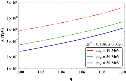
Figure 4: $\Lambda$ (in TeV) is plotted against $q$ for different $m_{\chi}$ and $\Omega h^{2}=0.1186\pm 0.0020$.

For a given $m_{\chi}$ all the three curves corresponding to three different values of $\Omega h^{2}$ are found to be almost overlapping. The following observations are in order: (a) For a given $m_{\chi}$, the upper bound on $\Lambda$ increases with the increase in $q$. As an example, for $m_{\chi}=30~{}\rm{MeV}$, $\Lambda$ changes from $4\times 10^{7}~{}\rm{TeV}$ to $1.6\times 10^{8}~{}\rm{TeV}$ as $q$ changes from $1.0$ to $1.1$ and (b) $\Lambda$ decreases with the increase in $m_{\chi}$ for a particular $q$. As an example, for $q=1.1$, we see that $\Lambda$ decreases from $4\times 10^{8}~{}\rm{TeV}$ to $1.1\times 10^{8}~{}\rm{TeV}$ as $m_{\chi}$ increases from $10$ to $50~{}\rm{MeV}$. In Fig. 5, we have ploted $\Omega h^{2}$ against the upper bound on $\Lambda$ (in TeV) for different mass fermion dark matter fermion for Case III in $q$-deformed (Fig. 5(a)) and undeformed (Fig. 5(b)) scenarios. In both figures the region below the horizontal lines $\Omega h^{2}=0.1186\pm 0.0020$ are allowed as this is the experimental upper bound on value of total non-baryonic contribution to the relic density.

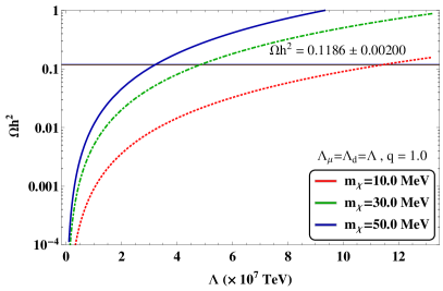
((a))

((b))

Figure 5: $\Omega h^{2}$ is plotted against $\Lambda$ (in TeV) for $q=1$ and $q=1.1$ and different $m_{\chi}$ values.

So theoretically estimated relic density for a particular particle produced in a particular process should not exceed the value $\Omega h^{2}=0.1186\pm 0.0020$, but can be less than or in extreme case equal to this. Fig. 5 suggests that for a given mass of DM fermions $m_{\chi}$ an increment in the value of the effective scale $\Lambda$ will cause a significant increment in the contribution to the relic density for that DM fermions. This observation is physically consistent as well. As $\Lambda$ increases, the coupling constants($\mu,d$) becomes weaker. As a result the DM couples more weakly to the concerned standard model(SM) paricles(here $e^{+}~{}\rm{and}~{}e^{-}$) and hence after their production, they are more likely to contribute to the relic density, rather than interacting with SM particles and gets scattered.

4.2 Discussion of the lower bound obtained from SN1987A Cooling(Raffelt’s criteria), Free Streaming(Optical depth criteria) with the upper bound obtained from the Relic density contribution

We find that the lower bound on $\Lambda$ obtained from the Raffelt’s criteria(SN1987A cooling), Optical depth criteria(free streaming of DM fermion) and the upper bound on $\Lambda$ obtained from the relic density contribution, obtained in both deformed and un-deformed scenarios are consistent with each other. The lower bound obtained on $\Lambda_{\mu}$ in undeformed scenario ($q=1.0$) is comparable with that obtained by Kadota et al.KS . Below in Table I, we make a comparative study of the lower and upper bounds on $\Lambda$ obtained by using the above three criteria.
Table I: The bound on the effective scale $\Lambda=\Lambda_{\mu}=\Lambda_{d}$ (TeV) (lower bound obtained from optical depth criterion, Raffelt’s criteria and upper bound obtained from relic density experimental value) are shown for different dark matter mass $m_{\chi}$ (MeV) in the undeformed($q=1$) and $q$-deformed scenario, for free streaming(optical depth criterion) there is a range of the reported value Atanu as it depends on the other supernova properties like temperature, densities etc. Dreiner ; DHLP ; Debades ; Das ; Ellis ; Lau ; Sathees ; Sumiyoshi ; Hagel ; FHS

	$m_{\chi}~{}(\rm{MeV})$	$\Lambda=\Lambda_{\mu}=\Lambda_{d}~{}\rm{(TeV)}$
		Free streaming	SN cooling	Relic bound
$q=1.0$	$10$	$\sim(3.6$-$10.5)\times 10^{7}$	$3.66\times 10^{6}$	$1.16\times 10^{8}$
	$30$	$\sim(3.6$-$10.5)\times 10^{7}$	$3.34\times 10^{6}$	$4.92\times 10^{7}$
	$50$	$\sim(3.6$-$10.5)\times 10^{7}$	$3.00\times 10^{6}$	$3.22\times 10^{7}$
$q=1.05$	$10$	$\sim(3.6$-$10.5)\times 10^{7}$	$1.25\times 10^{7}$	$1.76\times 10^{8}$
	$30$	$\sim(3.6$-$10.5)\times 10^{7}$	$1.2\times 10^{7}$	$5.37\times 10^{7}$
	$50$	$\sim(3.6$-$10.5)\times 10^{7}$	$1.15\times 10^{7}$	$7.73\times 10^{7}$
$q=1.1$	$10$	$\sim(3.6$-$10.5)\times 10^{7}$	$3.26\times 10^{7}$	$3.53\times 10^{8}$
	$30$	$\sim(3.6$-$10.5)\times 10^{7}$	$3.23\times 10^{7}$	$1.58\times 10^{8}$
	$50$	$\sim(3.6$-$10.5)\times 10^{7}$	$3.2\times 10^{6}$	$1.11\times 10^{8}$

In Fig. 6, we have shown the bounds on $\Lambda$ (in TeV) against the DM mass $m_{\chi}$ (in MeV) obtained from SN1987A energy loss rate (Raffelt’s criteria), Optical depth criterion(free streaming) and using Relic density of non-baryonic matter $\Omega h^{2}=0.1186$ (PDG 2017). We obtain lower bound from Raffelt’s criteria and Optical depth criterion and on the other hand we obtain upper bound using the maximum possible relic density of non-baryonic matter. Clearly, the region between the SN cooling and relic bound curves are allowed, forbidden regions are located below the SN cooling curve and above the relic curve. On the left the plots are shown for undeformed $q=1$ scenario, while on the right the plots are shown for $q=1.1$.

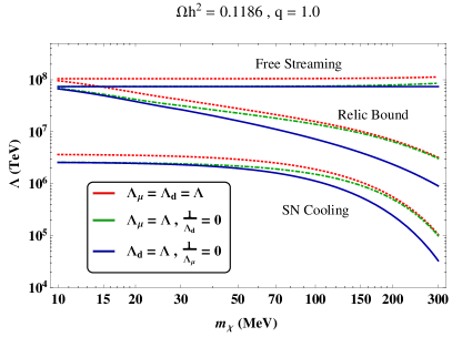
((a))

((b))

Figure 6: $\Lambda$(in TeV) (obtained from SN1987A cooling, free streaming Atanu and using Relic bound) is plotted against $m_{\chi}$(in MeV) for undeformed ($q=1$) and $q$-deformed scenario.

In Fig. 6(a)($q=1$ undeformed), we see that there is a widespread region between the lower bound on $\Lambda$ obtained from the SN1987A cooling criteria and the upper bound on $\Lambda$ obtained from the maximum possible value of relic density for an ultra-light mass $m_{\chi}=10$ MeV DM fermion, however the lower bound obtained from the free streaming criteria lies in the forbidden region. In the $q$-deformed scenario (with $q=1.1$) the story is slightly different(Fig. 6(b)). For a light mass dark matter (with $m_{\chi}$ ranging between $10$ MeV to $100$ MeV), the lower bounds obtained on $\Lambda$ from SN1987A cooling and free streaming criteria more-or-less agree with each other, but the upper bound differs by an order of magnitude obtained from the relic density constraint. For a heavier DM fermion with mass $m_{\chi}\sim 100~{}-~{}200$ MeV, the lower and upper bounds obtained from the supernovae cooling, free streaming criteria and relic density, are found to be comparable Atanu2 . This restricts or precisely forbids the production of heavier dark matter fermions inside supernova core as this is forbidden by the upper bound obtained from the relic density constraints.

5 Conclusion

The dark matter fermion produced inside the supernova SN1987A core in electron-positron collision $e^{+}e^{-}\rightarrow\chi\overline{\chi}$ , can take away the energy released in the supernova explosion and similar kind of dark matter fermion produced from some other sources as well can contribute to the relic density. Working within the formalism of $q$-deformed statistics we find the DM contribution to the relic density and using the experimental bound on the relic density (of the cold non-baryonic matter) $\Omega h^{2}=0.1186\pm 0.0020$ (obtained from the measurement of the anisotropy of the cosmic microwave background (CMB) and of the spatial distribution of galaxies), we obtain a upper bound on the effective scale $\Lambda$. In the un-deformed(deformed) scenario $q=1$($q=1.1$), for a light mass ($m_{\chi}=30$ MeV) dark matter, we find the upper bound on $\Lambda=4.9\times 10^{7}$ TeV($\Lambda=1.6\times 10^{8}$ TeV) from the relic density. This is consistent with the lower bound $3.3\times 10^{6}$ TeV($\Lambda=3.2\times 10^{7}$ TeV) obtained from the Raffelt’s criteria on the supernovae energy loss rate and $3.6\times 10^{7}$ TeV($\Lambda=3.6\times 10^{7}$ TeV) obtained from the optical depth criteria on the free streaming of the dark matter fermion in the un-deformed(deformed) scenario with $q=1$($q=1.1$), respectively. Here we can note one interesting fact that, for $q$-deformed scenario with $q=1.1$ both the lower bound curves of $\Lambda$ lies below the upper bound curves due to the relic density consideration which is physically consistent unlike the undeformed one($q=1.0$).

Appendix A From $q$-deformed statistics to undeformed scenario

In general, the distribution function for the $q$-deformed statistics is Tsallis

$$D_{i}=\left(1+\frac{b}{\tau}(E_{i}-\mu_{i})\right)^{\tau}+1$$ (33)

with $b=\frac{\beta_{0}}{4-3q}$, $\beta_{0}=\frac{1}{k_{B}T}$ (we work in the unit $k_{B}=1$) and $\tau=\frac{1}{q-1}$.

In terms of the dimensionless quantity $x_{i}=\frac{E_{i}}{T}$

$$D_{i}=\left(1+b(q-1)(Tx_{i}-\mu_{i})\right)^{\frac{1}{q-1}}+1$$ (34)

Now replacing $q-1$ by $m$, ($m\rightarrow 0$ as $q\rightarrow 1$)

$$\left(1+b(q-1)(Tx_{i}-\mu_{i})\right)^{\frac{1}{q-1}}=\left(1+bm(Tx_{i}-\mu_{i})\right)^{\frac{1}{m}}=y\mathrm{(say)}$$ (35)

Now

$$\lim_{m\rightarrow 0}y = \lim_{m\rightarrow 0}\left(1+bm(Tx_{i}-\mu_{i})\right)^{\frac{1}{m}}$$

$$\implies\lim_{m\rightarrow 0}\ln y = \lim_{m\rightarrow 0}{\frac{1}{m}}\ln\left(1+bm(Tx_{i}-\mu_{i})\right)$$

$$= \lim_{m\rightarrow 0}\frac{1}{1+bm(Tx_{i}-\mu_{i})}b(Tx_{i}-\mu_{i})$$

$$= b(Tx_{i}-\mu_{i})$$

Also for $q\rightarrow 1$, we find $b(=\frac{\beta_{0}}{4-3q})=\beta_{0}=\frac{1}{k_{B}T}=\frac{1}{T}$. So we find

$$\lim_{q\rightarrow 1}\ln y = \beta_{0}(Tx_{i}-\mu_{i})$$

$$\implies\lim_{q\rightarrow 1}y = \exp\left[\frac{1}{T}(Tx_{i}-\mu_{i})\right]$$

$$= \exp\left[x_{i}-\frac{\mu_{i}}{T}\right]$$

Clearly, in the undeformed scenario (i.e. $q=1$)

$$\lim_{q\rightarrow 1}D_{i}=\lim_{q\rightarrow 1}y+1=\exp\left[x_{i}-\frac{\mu_{i}}{T}\right]+1~{}~{}[Proved]$$ (36)

A.1 Feynman rules

Process: $e^{-}e^{+}\stackrel{{\scriptstyle\gamma}}{{\longrightarrow}}\chi\overline{\chi}$:

$e^{-}~{}e^{+}\rightarrow\gamma$  vertex: $ie\gamma^{\mu}$

$\gamma\rightarrow\chi~{}\overline{\chi}$  vertex: $i\left(\mu_{\chi}\sigma^{\mu\nu}q_{\nu}+d_{\chi}\sigma^{\mu\nu}q_{\nu}\gamma^{5}\right)$

- (1) M. Roos, “Dark Matter: The evidence from astronomy, astrophysics and cosmology,” 2010.
- (2) M. Roos, “Astrophysical and cosmological probes of dark matter,” J. Mod. Phys., vol. 3, p. 1152, 2012.
- (3) F. Zwicky, Helv. Phys. Acta 6, 110 (1933).
- (4) J. L. Feng, Ann. Rev. Astron. Astrophys. 48, 495 (2010).
- (5) G. Bertone, D. Hooper, J. Silk, Phys. Rep. 405, 279 (2005).
- (6) G. Jungman, M. Kamionkowski, K. Griest, Phys. Rep. 267, 195 (1996).
- (7) Atanu Guha, Selvaganapathy J and Prasanta Kumar Das, Phys. Rev. D 95, 015001 (2017).
- (8) G. G. Raffelt, Stars as Laboratories for Fundamental Physics (Chicago University Press, Chicago, 1996).
- (9) E.W. Kolb and M.S. Turner, The early universe, Addison Wesley (1990).
- (10) P. Gondolo and G. Gelmini, Nuclear Physics B360 (1991) 145-179.
- (11) D. Majumdar, Dark matter: An introduction, CRC Press, Taylor Francis Group, 2015.
- (12) Joakim Edsjö and Paolo Gondolo, Phys. Rev. D 56, 1879 (1997).
- (13) Paolo Gondolo and Graciela Gelmini, Phys. Rev. D 71, 123520 (2005).
- (14) C. Beck, E. G. D. Cohen, Physica (Amsterdam) 322A, 267 (2003).
- (15) G. Kaniadakis, Phys. Rev. E 66, 056125 (2002).
- (16) C. Beck, Eur. Phys. A 40, 267 (2009).
- (17) K. Hirata et al., Phys. Rev. Lett. 58, 1490 (1987).
- (18) R. M. Bionta et al., Phys. Rev. Lett. 58, 1494 (1987).
- (19) C. Tsallis, J. Stat. Phys. 52, 479 (1988).
- (20) Atanu Guha and Prasanta Kumar Das, Physica A: Statistical Mechanics and its Applications 495C (2018) pp. 18-29
- (21) Atanu Guha and Prasanta Kumar Das, Physica A: Statistical Mechanics and its Applications 497C (2018) pp. 272-284
- (22) Tsallis C 2009 Introduction to Nonextensive Statistical Mechanics: Approaching a complex World(Springer).
- (23) Nonextensive Statistical Mechanics and Its Applications, Sumiyoshi Abe Yuko Okamoto, (Lecture notes in physics ; Vol. 560), (Physics and astronomy online library), (Springer).
- (24) C. Beck, Physica (Amsterdam) 331A, 173 (2004).
- (25) I. Bediaga, E.M.F. Curado, J.M. de Miranda, Physica (Amsterdam) 286A, 156 (2000).
- (26) C. Beck, Physica A 286 (2000) 164.
- (27) C. Beck, Nonlinearity 8, 423 (1995).
- (28) C. Beck, Phys. Rev. D 69, 123515 (2004).
- (29) Kenji Kadota and Joseph Silk, Phys. Rev. D 89, 103528 (2014).
- (30) H. K. Dreiner, J. F. Fortin, C. Hanhart and L. Ubaldi, Phys. Rev. D 89, 105015 (2014).
- (31) H. K. Dreiner, C. Hanhart, U. Langenfeld and D. R. Phillips, Phys. Rev. D 68, 055004 (2003).
- (32) Prasanta Char, Sarmistha Banik and Debades Bandyopadhyay, Astrophys. J. 809, 116 (2015).
- (33) Prasanta Kr. Das, J. Selvaganapathy, Chandradew Sharma, Tarun Kumar Jha, V. Sunil Kumar, Int.J.Mod.Phys. A 28, 1350152 (2013).
- (34) J. R. Ellis, K. A. Olive, S. Sarkar and D. W. Sciama, Phys. Lett. B 215, 404 (1988).
- (35) K. Lau, Phys. Rev. D 47, 1087 (1993).
- (36) Prasanta Kumar Das, V. H. Satheeshkumar and P. K. Suresh, Phys. Rev. D 78, 063011 (2008).
- (37) Kohsuke Sumiyoshi and Gerd Ropke, Phys. Rev. C 77, 055804 (2008).
- (38) K. Hagel, J. B. Natowitz and G Röpke, Eur. Phys. J. A 50, 39 (2014).
- (39) P. Fayet, D. Hooper and G. Sigl., Phys. Rev. Lett. 96, 211302 (2006).
- (40) Atanu Guha and Prasanta Kumar Das, (work in progress).