Mott glass from localization and confinement

Abstract

We study a system of fermions in one spatial dimension with linearly confining interactions and short-range disorder. We focus on the zero temperature properties of this system, which we characterize using bosonization and the Gaussian variational method. We compute the static compressibility and ac conductivity, and thereby demonstrate that the system is incompressible, but exhibits gapless optical conductivity. This corresponds to a “Mott glass” state, distinct from an Anderson and a fully gapped Mott insulator, arising due to the interplay of disorder and charge confinement. We argue that this Mott glass phenomenology should persist to non-zero temperatures.

I Introduction

Rich phenomena arising from the interplay of disorder and interactions in quantum many-body systems have been at the center of considerable excitement over the past decade, particularly with the advent of many-body localization (MBL) Anderson (1958); Basko et al. (2006); Gornyi et al. (2005); Nandkishore and Huse (2015), a phenomenon whereby disordered interacting systems can exhibit ergodicity breaking and fail to equilibrate even at infinite times. While most theory in this field has been formulated for systems with short-range interactions, and long-range interactions are typically expected to suppress localization Levitov (1990); Burin (2006); Yao et al. (2014), a recent work Nandkishore and Sondhi (2017) introduced a model of one-dimensional (1D) linearly interacting fermions – the celebrated Schwinger model Schwinger (1962); Coleman (1976); Wolf and Zittartz (1985); Fischler et al. (1979) – with the additional ingredient of quenched disorder, argued to exhibit many-body localization despite its long-range interactions.

Here we study the ground state and low-energy properties of the disordered Schwinger model. While 1D non-interacting fermions in a random potentials localize, forming a gapless compressible Anderson insulator, a clean 1D system with Coulomb interaction exhibits charge confinement, with a fully gapped ground state. What are the ground state and low-energy properties when both of these ingredients are present, namely that of disordered linearly interacting fermions in one dimension?

Using bosonization and Gaussian variational method (GVM) Mézard and Parisi (1991); Giamarchi and Le Doussal (1996), here we explore the zero-temperature properties of this model and demonstrate that it realizes a distinct phase of matter, a “Mott glass” Orignac et al. (1999); Giamarchi et al. (2001), that is characterized by a hard gap in compressibility, but not in optical conductivity, i.e., it exhibits a vanishing compressibility and a finite ac conductivity down to zero frequency. The hard gap in compressibility arises due to confinement of charged excitations, while the absence of a hard gap in optical conductivity is due to the existence of random localized dipole excitations down to zero energy. Unlike previous explorations of such phenomena Orignac et al. (1999); Giamarchi et al. (2001); Weichman and Mukhopadhyay (2008); Vojta et al. (2016), Mott glass in the disordered Schwinger model is driven by the interplay of disorder and confinement from long-range interactions, and does not require a commensurate periodic potential Orignac et al. (1999). The model evades the compelling arguments against the Mott glass phase advanced in Ref. Nattermann et al., 2007 by way of its long-range interactions (a loophole that was anticipated in Ref. Nattermann et al., 2007).

While linearly confining interactions do not naturally arise in the solid state, the Schwinger model has been proposed Rico et al. (2014); Kühn et al. (2014); Notarnicola et al. (2015); Yang et al. (2016) and realized Martinez et al. (2016) in synthetic quantum systems. Furthermore, it has been extensively explored via numerical simulations Byrnes et al. (2002); Rico et al. (2014); Buyens et al. (2014); Bañuls et al. (2015); Saito et al. (2015); Bañuls et al. (2016); Buyens et al. (2016); Brenes et al. (2018); Kasper et al. (2017). The ideas advanced herein therefore admit near term tests both in numerics and in experiments with synthetic quantum matter.

The article is organized as follows. In Sec. II, we introduce the disordered Schwinger model and formulate its bosonized form. We then briefly review the GVM analysis in Sec. III. Readers familiar with these details may skip directly to Sec. IV, where the optical conductivity and static compressibility are calculated using the GVM, and Mott glass physics is demonstrated. We discuss the implications of our results and conclude in Sec. V.

II Model

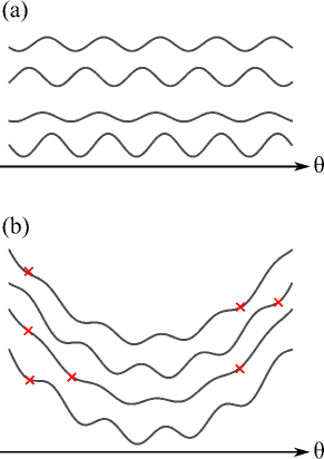
Figure 1: An ensemble of random boson potential in the disordered boson problems, with curves (offset for clarity) corresponding to different spatial points. (a) The Giamarchi-Schulz model exhibits a spatially random potential, that is periodic in the phonon displacement $\theta$, and is therefore characterized by an infinite number of minima. (b) In contrast, because of the fermionic long-range interactions a weakly disordered Schwinger model generically exhibits a unique minimum selected by the overall quadratic phonon potential. (Occasionally, the phonon potential develops doubly degenerate minima.) The red crosses indicate the local minima removed by the long-range fermionic interaction and the associated bosonic quadratic (in $\theta$) potential. The resulting ground state properties are qualitatively distinct from those of the conventional Bose glass, as we discuss in the main text.

We study a disordered Schwinger model Schwinger (1962); Coleman (1976) that describes electrons interacting via a dynamical gauge field in one spatial and one temporal dimension (1+1D). The gauge field induces a linearly-confining electron potential, corresponding to the Fourier transform of $1/k^{2}$, screened by a positive uniform ionic background (jellium model) and with the uniform translational zero mode $k=0$ suppressed by the boundary conditions. Integrating out the dynamical gauge field in the disorder-free Schwinger model leads to a strongly-interacting Hamiltonian $H_{0}+H_{\text{int}}$, where

$$H_{0}= v\int_{x}\left[R^{\dagger}\left(-i\partial_{x}R\right)-L^{\dagger}\left(-i\partial_{x}L\right)\right],$$ (1)

$$H_{\text{int}}= -e^{2}\int_{x,x^{\prime}}\,\rho_{0}(x)\left|x-x^{\prime}\right|\rho_{0}(x^{\prime}),$$ (2)

$\rho_{0}=R^{\dagger}R+L^{\dagger}L$ is the long-wavelength component of the density at average incommensurate filling, written in terms of the right ($R$) and left ($L$) moving chiral fermion, and above we defined $\int_{x}\equiv\int dx$. Utilizing standard bosonization Giamarchi (2004); Shankar (2017), the disorder-free Schwinger model is equivalently formulated in terms of an imaginary time path-integral with Euclidean action for a phonon-like field $\theta$ given by

$$\mathcal{S}_{0}= \int_{\tau,x}\left[\frac{1}{2\pi vK}\left((\partial_{\tau}\theta)^{2}+v^{2}\left(\partial_{x}\theta\right)^{2}\right)+\frac{2e^{2}}{\pi^{2}}\theta^{2}\right],$$ (3)

with the charge gap due to confinement characterized by a plasma frequency $\omega_{p}=2e\sqrt{vK/\pi}$ and a Luttinger parameter $K$, which accounts for short-range interactions.

The key additional ingredient that we include Nandkishore and Sondhi (2017) is the random impurities, modeled by a short-range correlated disorder potential. The latter can be expressed in terms of the long-wavelength forward-scattering ($H_{\text{imp},f}$) and the short-scale backscattering ($H_{\text{imp},b}$) parts Giamarchi and Schulz (1988), given by

$$H_{\text{imp},f}= \int_{x}\,\eta(x)\rho_{0}(x),$$ (4)

$$H_{\text{imp},b}= \int_{x}\,\left[\xi(x)L^{\dagger}R+\xi^{*}(x)R^{\dagger}L\right].$$ (5)

The corresponding random potentials, $\eta(x)$ (forward-scattering scalar potential) and $\xi(x)$ (back-scattering potential that is a random mass in the electronic representation Kogut and Susskind (1975); Byrnes et al. (2002)) are respectively real and complex zero-mean Gaussian random fields, characterized by

$$\overline{\eta(x)\,\eta(x^{\prime})}= \Delta_{f}\delta(x-x^{\prime}),\,\,\,\overline{\xi(x)\,\xi^{*}(x^{\prime})}=\Delta\delta(x-x^{\prime}),$$ (6)

$$\overline{\eta(x)\,\xi(x^{\prime})}= \overline{\xi(x)\,\xi(x^{\prime})}=0,$$ (7)

where $\overline{\mathcal{O}}$ denotes disorder average of $\mathcal{O}$.

The forward-scattering component of disorder bosonizes to $\int_{\tau,x}\,\eta(x)\,\frac{1}{\pi}\partial_{x}\theta$ in Euclidean action, and (since it is linear in $\theta$) can be safely eliminated from the action by a shift in $\theta$ linear in $x$ (see discussions in Appendix. A), and for our purposes can thus be safely neglected as in the conventional localization problem Giamarchi and Schulz (1988). In contrast, the back-scattering disorder plays a crucial role and leads to localization. Integrating over disorder using a replica “trick” Edwards and Anderson (1975) (in equilibrium equivalent to the Keldysh path integral), generates a short-range disorder component of the replicated action,

$$\mathcal{S}_{\text{dis}}=-\tilde{\Delta}\sum_{a,b}\int_{x,\tau,\tau^{\prime}}\cos\left[2\theta_{a}(\tau,x)-2\theta_{b}(\tau^{\prime},x)\right],$$ (8)

where $\tilde{\Delta}=\Delta/(2\pi^{2}\alpha^{2})$, $a$ and $b$ are replica indices, and $\alpha$ is the microscopic ultra-violet length scale, set for example by the disorder correlation length or the underlying lattice constant.

Because long-range Coulomb interaction strongly suppresses charge fluctuations (see Fig. 1), gapping out $\theta$, in contrast to randomly pinned acoustic systems Fisher et al. (1989) and short-range interacting disordered electrons (as studied by e.g., Giamarchi-Schulz Giamarchi and Schulz (1988)) the back-scattering disorder in the Schwinger model is strongly relevant for all values of parameters,

$$\frac{d\tilde{\Delta}}{dl}=3\tilde{\Delta}.$$ (9)

Our interest is in the ground state and low-energy excitations of the disordered Schwinger model, where fermions are confined by the linear potential, and bosonic excitations are localized by disorder Nandkishore and Sondhi (2017). The strong relevance of disorder thus requires a nonperturbative treatment in $\Delta$, to which we turn next.

III Gaussian Variational Method

We now analyze the low-energy properties of the model defined by $\mathcal{S}=\mathcal{S}_{0}+\mathcal{S}_{\text{dis}}$ [Eqs. (3) and (8)], utilizing a nonperturbative but generally uncontrolled GVM Mézard and Parisi (1991); Giamarchi and Le Doussal (1996) . The basic idea is to approximate the Schwinger nonlinear action by the “best” harmonic action, with optimized variational parameters determined by the minimum of the variational ground state energy. The resulting quadratic variational action then allows a computation of physical observables, with our focus here on the optical conductivity and static compressibility, that characterize the disordered Schwinger ground state and its low-energy excitations.

The GVM is known to capture the basic low-temperature properties of Bose glass in the Giamarchi-Schulz model Giamarchi and Le Doussal (1996). Because the Schwinger model is gapped by long-range interactions, cutting off long-scales (that are otherwise challenging to handle) by the inverse of the plasma frequency, $1/\sqrt{\omega_{p}}$, we in fact expect the GVM to be both qualitatively and quantitatively accurate for the problem at hand, at least for weak disorder.

To this end, we consider a general imaginary time action $\mathcal{S}$ which can be separated into two parts, $\mathcal{S}=\mathcal{S}_{\text{var}}+\delta\mathcal{S}$, where $\mathcal{S}_{\text{var}}$ is a variational quadratic action. $\delta\mathcal{S}=\mathcal{S}-\mathcal{S}_{\text{var}}$ is a perturbation around $\mathcal{S}_{\text{var}}$. The partition function is formally expressed as

$$Z=\int\mathcal{D}\theta\,e^{-\mathcal{S}_{\text{var}}[\theta]-\delta\mathcal{S}[\theta]}=Z_{0}\left\langle e^{-\delta\mathcal{S}[\theta]}\right\rangle_{\text{var}},$$ (10)

where $\langle\mathcal{O}\rangle_{\text{var}}$ denotes the expectation value of $\mathcal{O}$ with respect to $\mathcal{S}_{\text{var}}$. Accordingly, the free energy is given by

$$F= -T\ln Z_{\text{var}}-T\ln\left[\left\langle e^{-\delta\mathcal{S}}\right\rangle_{\text{var}}\right]$$ (11)

$$\leq -T\ln Z_{\text{var}}-T\left\langle\delta\mathcal{S}\right\rangle_{\text{var}}\equiv F_{\text{var}},$$ (12)

where $F_{\text{var}}$ is a variational free energy functional to leading order in $\delta\mathcal{S}$, that by convexity of the exponential function is a strict upper bound for the actual free energy $F$ Feynman (1998); Chaikin and Lubensky (2000). Although this can be extended to an improved variational free energy upper bound as a cumulant expansion in $\delta\mathcal{S}$, here we limit our analysis to above lowest order, as it is sufficient for our purposes here. The optimal $\mathcal{S}_{\text{var}}$ upper bound is set by minimizing the variational free energy $F_{\text{var}}$.

For the disordered Schwinger model, we consider the replicated disorder-averaged action, $\mathcal{S}=\mathcal{S}_{\text{var}}+\mathcal{S}_{\text{dis}}$. The inter- and intra- replica correlation functions need to be treated as independent functions. Even though only the intra-replica response function is directly related to physical observables, correlation functions are determined by an inverse of the replica matrix kernel and thus depend on all of its components. The general variational quadratic action is given by:

$$\mathcal{S}_{\text{var}}= \frac{1}{2\beta L}\sum_{a}\sum_{\omega_{n},k}G^{-1}_{aa}(\omega_{n},k)\theta_{a}(-\omega_{n},-k)\theta_{a}(\omega_{n},k)$$

$$+\frac{1}{2\beta L}\sum_{a,b,(a\neq b)}\sum_{\omega_{n},k}G^{-1}_{ab}(\omega_{n},k)\theta_{a}(-\omega_{n},-k)\theta_{b}(\omega_{n},k),$$ (13)

where $a$, $b$ denote replica indices, $\beta$ is the inverse temperature, and $L$ is the system size. The intra-replica $(G_{aa})$ and inter-replica $(G_{a\neq b})$ Green functions are independent variational parameters.

With this set up, the variational free energy $F_{var}=F_{0}+F_{1}+F_{\text{dis}}$ is then formally given by,

$$F_{0}= -\frac{1}{2\beta}\sum_{a}\sum_{\omega_{n},k}\ln\left[G(\omega_{n},k)\right]_{aa},$$ (14)

$$F_{1}= \frac{1}{2v\pi K\beta}\sum_{a}\sum_{\omega_{n},k}\left(\omega_{n}^{2}+v^{2}k^{2}+\frac{4e^{2}vK}{\pi}\right)G_{aa}(\omega_{n},k),$$ (15)

$$F_{\text{dis}}= -\tilde{\Delta}\int_{\tau,x}\left[\sum_{a,b}e^{-2\left\langle\left(\theta_{a}(\tau,x)-\theta_{b}(0,x)\right)^{2}\right\rangle_{\text{var}}}\right].$$ (16)

where $F_{0}$ is the free energy corresponding to the harmonic variational action $\mathcal{S}_{\text{var}}$, $F_{1}$ and $F_{\text{dis}}$ come from $-T\langle\left(\mathcal{S}_{0}-\mathcal{S}_{\text{var}}\right)\rangle_{\text{var}}$ and $-T\langle\mathcal{S}_{\text{dis}}\rangle_{\text{var}}$ contributions, respectively, and we have dropped an unimportant additive constant. The bosonic correlator in Eq. (16) is straightforwardly computed to be given by

$$\left\langle\left(\theta_{a}(\tau,x)-\theta_{b}(0,x)\right)^{2}\right\rangle_{\text{var}}$$

$$= \frac{1}{\beta L}\sum_{\omega_{n},k}\left[G_{aa}(\omega_{n},k)+G_{bb}(\omega_{n},k)-2\cos\left(\omega_{n}\tau\right)G_{ab}(\omega_{n},k)\right].$$ (17)

We then carry out a functional derivative of $F_{var}$ with respect to the variational parameters, $G_{ab}(\omega_{n},k)$. The saddle point equation is thereby given by

$$G^{-1}_{ab}= \left[\frac{1}{v\pi K}\left(\omega_{n}^{2}+v^{2}k^{2}\right)+\frac{4e^{2}}{\pi^{2}}\right]\delta_{ab}$$

$$+4\tilde{\Delta}\sum_{cd}\int_{\tau}\bigg{\{}\!\left[\delta_{ab}\delta_{ac}+\delta_{ab}\delta_{ad}-2\delta_{ac}\delta_{bd}\cos\left(\omega_{n}\tau\right)\right]$$

$$\hskip 11.38092pt\times e^{-\frac{2}{\beta L}\sum\limits_{\nu_{n},k}\left[G_{cc}(\nu_{n},q)+G_{dd}(\nu_{n},q)-2\cos\left(\nu_{n}\tau\right)G_{cd}(\nu_{n},q)\right]}\bigg{\}}.$$ (18)

and determines the optimum value of the variational parameters. The explicit derivation is standard but lengthy, with details found in the literature Giamarchi and Le Doussal (1996); Orignac et al. (1999); Giamarchi et al. (2001) and specific to the disordered Schwinger model in Appendix. B.

Before turning to the computation of the Green function and the associated physical predictions, we highlight key technical components of the analysis. In the replica formalism, the inter-replica correlations are time-independent Giamarchi and Le Doussal (1996). Consequently, $G^{-1}_{a\neq b}(\omega_{n},k)$ is only non-zero at $\omega_{n}=0$. Another important detail is that the optimum variational solution is given by a replica symmetry broken structure, with $G^{-1}_{ab}$ for $a\neq b$ given by a hierarchical structure Mézard and Parisi (1991); Giamarchi and Le Doussal (1996). For 1D disordered fermions, it has been demonstrated that a one-step replica symmetry broken solution is sufficient, and the marginal stability condition is adopted Giamarchi and Le Doussal (1996).

For the disordered Schwinger model, the variational ansatz is the same as that previously used in Refs. Orignac et al., 1999 and Giamarchi et al., 2001 for their putative, substrate-driven Mott glass Nattermann et al. (2007), except that here the boson mass is (not a variational parameter but is) physical, determined by the plasma frequency associated by the confining Coulomb interaction. We separate the intra-replica Green functions into the finite-frequency ($\omega_{n}\neq 0$) and zero-frequency ($\omega_{n}=0$) components. The former is given by a diagonal matrix in the replica space. The latter is derived by inverting a hierarchical matrix in the replica space Mézard and Parisi (1991). The Green function is therefore non-analytic at zero frequency. For finite frequencies, the intra-replica correlation function is given by

$$G_{aa}(\omega_{n}\neq 0,k)= \frac{1}{\frac{1}{\pi vK}\left(\omega_{n}^{2}+v^{2}k^{2}\right)+\frac{4e^{2}}{\pi^{2}}+\Sigma+I(\omega_{n})},$$ (19)

where $\Sigma+I(\omega_{n})$ is the bosonic self energy, with $\Sigma$ its zero-frequency component, and $I(\omega_{n})$ determines the frequency dependence of the self energy, and is crucial for response functions like optical conductivity. $I(\omega_{n})$ has the following important asymptotic behaviors,

$$I(\omega_{n})\sim\begin{cases}\frac{2}{\sqrt{3}}\sqrt{\frac{1}{v\pi K}\left(\Sigma+\frac{4e^{2}}{\pi^{2}}\right)}|\omega_{n}|,&\text{for }\omega_{n}\rightarrow 0,\\[5.69054pt] 2\left(\Sigma+\frac{4e^{2}}{\pi^{2}}\right)\left[1-\frac{\sqrt{v\pi K\left(\Sigma+\frac{4e^{2}}{\pi^{2}}\right)}}{|\omega_{n}|}\right],&\text{for }\omega_{n}\rightarrow\infty.\end{cases}$$ (20)

We obtain the full frequency dependence of $I(\omega_{n})$ by solving Eq. (57) derived from GVM Giamarchi and Le Doussal (1996).

For $\omega_{n}=0$, the intra-replica Green function takes a different form from Eq. (19) and is given by

$$G_{aa}(\omega_{n}=0,k)=\frac{1/u_{c}}{\frac{v}{\pi K}k^{2}+\frac{4e^{2}}{\pi^{2}}}+\frac{1-1/u_{c}}{\frac{v}{\pi K}k^{2}+\Sigma+\frac{4e^{2}}{\pi^{2}}},$$ (21)

where $u_{c}\in[0,1]$ [determined by Eq. (56)] is a parameter of the one-step replica symmetry broken ansatz.

We thus find that the variational solution of the disordered Schwinger model displays a form (finite boson mass) similar to that of the putative Mott glass state, proposed in Refs. Orignac et al., 1999 and Giamarchi et al., 2001. However, here the ever-present charge confinement ensures that the boson mass is always nonzero, and thus the disordered Schwinger model does not exhibit a transition to an Anderson insulator (vanishing mass) or a fully gapped insulator ($\Sigma=0$) in the thermodynamic limit. As we will see in the next section, for all ranges of parameters at zero temperature it displays the phenomenology of and therefore realizes the Mott glass phase proposed in Ref. Orignac et al., 1999, but without requiring a commensurate lattice potential, and evading arguments in Ref. Nattermann et al., 2007.

IV Response Functions

The universal behavior of physical observables can be used to define and distinguish qualitatively distinct phases. For example, combining the results of optical conductivity and static compressibility, one can distinguish metals, gapped insulators, and Anderson insulators. Here we study the optical conductivity and the compressibility of the disordered Schwinger model, and demonstrate below that indeed they exhibit qualitative behavior consistent with the Mott glass phase envisioned in Refs. Orignac et al., 1999 and Giamarchi et al., 2001. We will then also discuss the implications for the low-temperature states based on the Mott glass phenomenology.

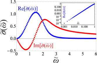
Figure 2: Dimensionless optical conductivity in the ground state of the disordered Schwinger model given by Eq. (23). The dimensionless quantities are defined by $\tilde{\sigma}(\tilde{\omega})=\pi^{2}\sigma(\omega)/\sqrt{\frac{v\pi K}{\Sigma^{\prime}}}$ and $\tilde{\omega}=\omega\sqrt{\frac{1}{v\pi K\Sigma^{\prime}}}$. $\Sigma^{\prime}=\Sigma+\frac{4e^{2}}{\pi^{2}}$. The blue (red) dots denote the real (imaginary) part of the $\tilde{\sigma}(\tilde{\omega})$. The real part of the optical conductivity does not contain a hard gap but displays a power law $\text{Re}\left[\tilde{\sigma}(\tilde{\omega})\right]\propto\tilde{\omega}^{2}$ behavior in the low frequency limit, as illustrated in the inset. The optical conductivity is consistent with that of a localized insulator. Inset: The low frequency real part of the conductivity, displays $\omega^{2}$ behavior.

IV.1 Optical Conductivity

To compute linear optical conductivity, we use Kubo formula and analytic continuation to real frequency of the intra-replica correlation functions. The optical conductivity is thus given by

$$\sigma(\omega)=\frac{1}{\pi^{2}}\frac{i}{\omega+i\delta}\left[\omega_{n}^{2}\left\langle\theta\theta\right\rangle(\omega_{n},k=0)\right]_{i\omega_{n}\rightarrow\omega+i\delta},$$ (22)

with $\delta\rightarrow 0^{+}$. The associated $\theta$ phonon correlator above is straightforwardly computed using the optimized quadratic variational action based on GVM. Using this correlator and Eqs. (19) and (22), the optical conductivity is then given by

$$\sigma(\omega)= \frac{1}{\pi^{2}}\frac{i}{\omega+i\delta}\left[\frac{-\omega^{2}}{\frac{-1}{v\pi K}\omega^{2}+\frac{4e^{2}}{\pi^{2}}+\Sigma+I(-i\omega)}\right]$$ (23)

$$= \frac{-i\omega}{\pi^{2}}\frac{\frac{-\omega^{2}}{v\pi K}+\Sigma^{\prime}+\text{Re}[I(-i\omega)]-i\text{Im}[I(-i\omega)]}{\left(\frac{-\omega^{2}}{v\pi K}+\Sigma^{\prime}+\text{Re}[I(-i\omega)]\right)^{2}+\left(\text{Im}[I(-i\omega)]\right)^{2}},$$ (24)

where $\Sigma^{\prime}=\Sigma+\frac{4e^{2}}{\pi^{2}}$. The finite frequency dependence of $\sigma(\omega)$ is determined by $I(-i\omega)$. The full frequency profile of the optical conductivity is plotted in Fig. 2. We focus on low and high frequency asymptotic dependences characterizing the Mott glass phase, that can be worked out via Eqs. (20) and (24).

In the low frequency limit, the real and imaginary part of conductivity give

$$\text{Re}[\sigma(\omega)]\approx \frac{1}{\pi^{2}}\frac{\sqrt{\frac{1}{v\pi K}}}{\left(\Sigma+\frac{4e^{2}}{\pi^{2}}\right)^{3/2}}\frac{2}{\sqrt{3}}\omega^{2},$$ (25)

$$\text{Im}[\sigma(\omega)]\approx \frac{-1}{\pi^{2}}\frac{\omega}{\Sigma+\frac{4e^{2}}{\pi^{2}}}.$$ (26)

The low temperature conductivity behavior is consistent with the previous GVM analysis for Bose glass models in one dimension Giamarchi and Le Doussal (1996); Orignac et al. (1999); Giamarchi et al. (2001) and coincides with the states deep in many-body localized phase Gopalakrishnan et al. (2015) (for a different reason, presumably). It is consistent with the gapless compressible Anderson insulator, with the optical conductivity characterized by a low-frequency power law down to zero frequency Mott (1968). In one dimension, it is given by $\omega^{2}$ upto logarithmic corrections Mott (1968); Berezinskii (1974). Indeed the GVM gives $\omega^{2}$ behavior, but cannot resolve logarithmic correction in the low frequency limit. We emphasize that the low frequency $\omega^{2}$ dependence is determined by $I(-i\omega)$ in Eq. (24). In contrast, a fully gapped Mott or band insulator below a gap is characterized by $I(-i\omega)=0$, displaying a hard gap in the optical conductivity.

In the high frequency limit (still in a localized regime), the real and imaginary parts of conductivity give

$$\text{Re}[\sigma(\omega)]\approx \frac{2\sqrt{\pi}(vK)^{5/2}}{\omega^{4}}\left(\Sigma+\frac{4e^{2}}{\pi^{2}}\right)^{3/2},$$ (27)

$$\text{Im}[\sigma(\omega)]\approx \frac{vK}{\pi}\frac{1}{\omega}.$$ (28)

In the Giamarchi-Schulz model, this tail in the real part of conductivity reproduces the perturbative result, $\text{Re}[\sigma(\omega)]\sim\omega^{-4+2K}$ Giamarchi (2004), by considering finite temperature and weak disorder in GVM Giamarchi and Le Doussal (1996). In the disordered Schwinger model, the strongly relevant renormalization group flow of the backscattering disorder [given by Eq. (9)] is independent of the Luttinger parameter, thereby effectively corresponding to $K=0$. We therefore predict the $\omega^{-4}$ high frequency tail in the non-zero (low) temperature limit.

IV.2 Compressibility

A complementary characterization of the state is via the static compressibility, that is nonzero for a compressible Anderson insulator, and zero for an incompressible gapped Mott insulator.

Within GVM, the compressibility of the disordered Schwinger model is straightforwardly computed from the static density-density correlation function,

$$D(k)= \frac{k^{2}}{\pi^{2}}\left\langle\theta(\omega=0,-k)\,\theta(\omega=0,k)\right\rangle$$ (29)

$$= k^{2}\left[\frac{1/u_{c}}{\frac{v}{\pi K}k^{2}+\frac{4e^{2}}{\pi^{2}}}+\frac{1-1/u_{c}}{\frac{v}{\pi K}k^{2}+\Sigma+\frac{4e^{2}}{\pi^{2}}}\right],$$ (30)

where we have used the zero-frequency Green function given by Eq. (21) from GVM. As advertised in the Introduction, we thus find that the static compressibility of the disordered Schwinger model, $\chi_{s}\propto\lim\limits_{k\rightarrow 0}D(k)=0$, vanishes, displaying a charge gap associated with confinement. Namely, $\chi_{s}$ would remain be finite in the absence of $4e^{2}/\pi^{2}$ in Eq. (29). This result appears to be in conflict with our results for optical conductivity (which contains no hard gap). In the next subsection we will discuss the differences between the two response functions, arguing that this is a consistent characterization of the Mott glass phase, intermediate between and sharply distinct from a fully compressible Anderson and a fully incompressible Mott insulator.

IV.3 Mott Glass Phenomenology

The ground state of the disordered Schwinger model simultaneously exhibits localization and confinement. Above we have demonstrated above, its low-frequency optical conductivity displays $\omega^{2}$ behavior, a hallmark of a localized insulator in one dimension Mott (1968); Berezinskii (1974). On the other hand, we found that its static compressibility vanishes, characteristic of a fully gapped incompressible insulator. This unconventional ground state is thus a Mott glass Orignac et al. (1999); Giamarchi et al. (2001); Weichman and Mukhopadhyay (2008), characterized by gapped single particle and gapless particle-hole excitations. In the presence of disorder, the particle-hole excitations appear at arbitrary low energies but remain localized in space. Giamarchi et al. (2001); Nandkishore and Sondhi (2017). These localized excitons dominate the optical conductivity at low frequencies, while the static compressibility vanishes due to the absence of low energy charged (single particle) excitations.

This intermediate Mott glass phenomenology naturally characterizes the ground state of disordered fermions with confinement of charges driven by long-range interaction. We conjecture that Mott glass may also extend to non-zero temperature states (putatively MBL Nandkishore and Sondhi (2017)) as we now discuss.

Firstly, confinement is a property of the entire spectrum, not just the ground state. We therefore expect that the static density-density correlation function $D(k\rightarrow 0)$ [given by Eq. (29)] is vanishingly small even at the non-zero energy-density many-body states. Although it is difficult to infer much about the finite energy density MBL states based on the GVM results, it is generally believed that the optical conductivity in MBL gives $\omega^{\alpha}$ where $\alpha$ is a continuously varying exponent between 1 and 2 Gopalakrishnan et al. (2015). For states deep inside the MBL phase, $\omega^{2}$ behavior is expected. Given the arguments of Ref. Nandkishore and Sondhi, 2017, indicating that the disordered Schwinger model is many-body localized at non-zero energy density (at least insofar as states can be many-body localized in the continuum Aleiner et al. (2010); Nandkishore (2014); Gornyi et al. (2017)), we conjecture that Mott glass phenomenology of a disordered Schwinger model also extends to non-zero temperature.

Finally, it is interesting to consider the effect of a uniform background electric field, $E_{0}$, that can be included by adding $\sim\int_{x,\tau}eE_{0}x\rho_{0}(x)$ to the action. Bosonizing $\rho_{0}(x)=\frac{1}{\pi}\partial_{x}\theta$ and integrating by parts, it is clear that an electric field appears as $-\int_{x,\tau}eE_{0}\theta$, and can be shifted away (along with the forward scattering), leaving the disorder-averaged action $\mathcal{S}_{0}+\mathcal{S}_{\text{dis}}$ unchanged. Therefore, in contrast to the conventional Schwinger model studied by Coleman Coleman (1976), consistent with Imry-Wortis Imry and Wortis (1979) arguments, in a disordered Schwinger model we do not expect a uniform electric field to induce a phase transition.

V Discussion and Conclusion

We have studied a disordered Schwinger model, describing one-dimensional, long-range interacting relativistic fermions in the presence of a random potential. We find that the model exhibits a localized state, despite its long-range interactions. We study its properties and compute its optical conductivity and static compressibility within the Gaussian replica variation analysis. We find that the system shows an incompressible localized glass state, with low-frequency conductivity scaling with $\omega^{2}$. We thus show that such a system indeed displays properties akin to a putative Mott glass state, previously proposed in a different context in the literatureOrignac et al. (1999); Giamarchi et al. (2001).

By way of long-range confining interactions the present system sidesteps forceful arguments against the existence of Mott glass, advanced in Ref. Nattermann et al., 2007. Our results indicate that the Mott glass phenomenology (gapped single-particle and gapless localized particle-hole excitations) is a natural consequence of the simultaneous presence of localization and confinement. Whether this phenomenology persists in more complicated disordered confined systems (perhaps in higher dimensions) is an intriguing question for future work.

We furthermore conjecture that Mott glass remains stable at non-zero temperatures, up to small corrections associated with fragility of MBL in the continuum Aleiner et al. (2010); Nandkishore (2014); Gornyi et al. (2017).

While the linearly confining potential does not naturally arise in conventional solid state materials, the Schwinger model may be realized and studied in the synthetic quantum many-body systems Rico et al. (2014); Kühn et al. (2014); Notarnicola et al. (2015); Yang et al. (2016); Martinez et al. (2016); Kasper et al. (2017). Numerical simulations Byrnes et al. (2002); Rico et al. (2014); Buyens et al. (2014); Bañuls et al. (2015); Saito et al. (2015); Bañuls et al. (2016); Buyens et al. (2016); Brenes et al. (2018) also provide a route to explore this interesting model and to test our predictions for its phenomenology.

Appendix A Spatially-dependent Scalar Potential

In this Appendix, we demonstrate how forward scattering potential in $\mathcal{S}_{0}+\mathcal{S}_{\eta}$ can be eliminated by a simple time-independent shift of the phonon field $\theta(x,\tau)\rightarrow\theta(x,\tau)+\zeta(x)$. Under this transformation the action becomes $\mathcal{S}^{\prime}$

$$\mathcal{S}^{\prime}= \mathcal{S}_{0}+\int d\tau dx\frac{2v^{2}}{2v\pi K}\left(\partial_{x}\theta\right)\left(\partial_{x}\zeta\right)$$

$$+\int d\tau dx\frac{2M^{2}}{2\pi}\theta\zeta+\int d\tau dx\,\eta(x)\frac{1}{\pi}\partial_{x}\theta,$$ (31)

where we have dropped unimportant, $\theta$-independent constant. We then require a vanishing of the terms linear in $\theta$, ensured by by a choice of the shift $\zeta(x)$ field satisfying a saddle point equation

$$\partial_{x}^{2}\zeta-\frac{KM^{2}}{v}\zeta=-\frac{K}{v}\partial_{x}\eta(x).$$ (32)

Under the physical condition of $\zeta(\pm\infty)=0$, the solution is then simply given by

$$\zeta(x)= \int dx^{\prime}\frac{e^{-M\sqrt{K/v}|x-x^{\prime}|}}{2M\sqrt{K/v}}\left[-\frac{K}{v}\partial_{x^{\prime}}\eta(x^{\prime})\right].$$ (33)

Appendix B Variational Free Energy and Saddle Point Equations

In this appendix, for completeness we sketch the solution of Eq. (18), following the analysis in Ref. Giamarchi and Le Doussal, 1996.

To begin, we define the self-energy $\chi_{ab}$ via

$$G^{-1}_{ab}(\omega_{n},k)= \left[\frac{\omega_{n}^{2}+v^{2}k^{2}}{v\pi K}+\frac{M^{2}}{\pi}\right]\delta_{ab}-\chi_{ab}(\omega_{n},k),$$ (34)

where $M^{2}=4e^{2}/\pi$. It is also useful to define a quantity $G_{C}^{-1}=\sum_{b}G^{-1}_{ab}$, which satisfies the saddle point equation,

$$G_{C}^{-1}(\omega_{n},k)= \frac{1}{v\pi K}\left(\omega_{n}^{2}+v^{2}k^{2}\right)+\frac{M^{2}}{\pi}$$

$$+8\tilde{\Delta}\!\int d\tau\Bigg{\{}\!\left[1-\cos\left(\omega_{n}\tau\right)\right]$$

$$\hskip 42.67912pt\times\left[e^{-2B_{aa}(\tau)}+\!\sum\limits_{b,(b\neq a)}\!e^{-2B_{ab}(\tau)}\right]\!\Bigg{\}},$$ (35)

$$\chi_{a\neq b}(\omega_{n},k)= 8\tilde{\Delta}\int d\tau\cos\left(\omega_{n}\tau\right)e^{-2B_{ab}(\tau)},$$ (36)

where

$$B_{aa}(\tau)= \frac{2}{\beta L}\sum_{\omega_{n},k}\left[G_{aa}(\omega_{n},k)-\cos(\omega_{n}\tau)G_{aa}(\omega_{n},k)\right],$$ (37)

$$B_{a\neq b}(\tau)= \frac{2}{\beta L}\sum_{\omega_{n},k}\left[G_{aa}(\omega_{n},k)-\cos(\omega_{n}\tau)G_{ab}(\omega_{n},k)\right]$$ (38)

$$= \frac{2}{\beta L}\sum_{\omega_{n},k}\left[G_{aa}(\omega_{n},k)-\delta_{\omega_{n},0}G_{ab}(0,k)\right].$$ (39)

Above we have used the symmetry $G_{ab}=G_{ba}$ and constancy of the diagonal elements. We also note that, $B_{a\neq b}$ is independent of $\tau$ Giamarchi and Le Doussal (1996).

In order to compute the saddle point equations in the required zero-replica limit, we adopt Parisi’s parametrization Mézard and Parisi (1991) as follows:

$$A_{aa}\rightarrow\tilde{A},\,\,\,A_{a\neq b}\rightarrow A(u),$$ (40)

where $\tilde{A}$ is the intra-replica element and $u\in[0,1]$ is a continuous parameter that encodes the inter-replica structure in $A(u)$. Specifically, we consider one-step replica symmetry broken ansatz which corresponds to $A(u<u_{c})=A_{0}$ and $A(u\geq u_{c})=A(u_{c})$. $u_{c}$, describing the break point of $u$ is also a variational parameter in GVM. We also adopt the algebraic rules of the hierarchical matrices in Ref. Mézard and Parisi, 1991.

The saddle point equations [Eqs. (35) and (36)] in the zero-replica limit become to

$$G_{C}^{-1}(\omega_{n},k)= \frac{1}{v\pi K}\left(\omega_{n}^{2}+v^{2}k^{2}\right)+\frac{M^{2}}{\pi}$$

$$+8\tilde{\Delta}\int d\tau\left[1-\cos\left(\omega_{n}\tau\right)\right]$$

$$\hskip 28.45274pt\times\left[e^{-2\tilde{B}(\tau)}-\int_{0}^{1}du\,e^{-2B(u)}\right],$$ (41)

$$\chi(\omega_{n};u)= 8\tilde{\Delta}\int d\tau\cos\left(\omega_{n}\tau\right)e^{-2B(u)}$$

$$= 8\tilde{\Delta}\beta\delta_{\omega_{n},0}e^{-2B(u)}\equiv\delta_{\omega_{n},0}\chi(u)$$ (42)

where

$$\tilde{B}(\tau)= \frac{2}{\beta L}\sum_{\nu_{n},q}\left[\tilde{G}(\nu_{n},q)-\cos\left(\nu_{n}\tau\right)\tilde{G}(\nu_{n},q)\right],$$ (43)

$$B(u)= \frac{2}{\beta L}\sum_{\nu_{n},q}\left[\tilde{G}(\nu_{n},q)-\delta_{\nu_{n},0}G(\nu_{n},q;u)\right].$$ (44)

We note that the summation over inter-replica elements turns into an integration over $u$ with an overall minus sign due to zero-replica limit. The inter-replica correlations vanish for non-zero Matsubara frequencies Giamarchi and Le Doussal (1996). Therefore, we can simply invert the Green function $G^{-1}_{C}(\omega_{n}\neq 0,k)=[G_{C}(\omega_{n}\neq 0,k)]^{-1}$. We express $\tilde{B}(\tau)$ and $B(u)$ as follows:

$$\tilde{B}(\tau)= \frac{2}{\beta L}\sum_{\nu_{n},q}\left[1-\cos\left(\nu_{n}\tau\right)\right]G_{C}(\nu_{n},q),$$ (45)

$$B(u)= \frac{2}{\beta L}\sum_{\nu_{n}\neq 0,q}G_{C}(\nu_{n},q)$$

$$+\frac{2}{\beta L}\sum_{q}\left[\tilde{G}(\nu_{n}=0,q)-G(\nu_{n}=0,q;u)\right].$$ (46)

For one-step replica symmetry broken ansatz, we consider Giamarchi and Le Doussal (1996); Orignac et al. (1999); Giamarchi et al. (2001)

$$\chi(u)=\begin{cases}\chi(u_{c}),&\text{ for }u_{c}\geq u,\\ 0,&\text{ for }u_{c}<u.\end{cases}$$ (47)

Correspondingly,

$$B(u)=\begin{cases}B,&\text{ for }u_{c}\geq u,\\ \infty,&\text{ for }u_{c}<u.\end{cases}$$ (48)

The Green functions [$G_{C}(\omega_{n},k)$, $\tilde{G}(\omega_{n},k)$, and $G(\omega_{n},k;u)$ ] depend on $\chi(u)$. We introduce self-energy parameters $\Sigma$ and $I(\omega_{n})$ to encode the interacting Green functions,

$$G_{C}^{-1}(\omega_{n},k)= \frac{1}{\pi vK}\left(\omega_{n}^{2}+v^{2}k^{2}\right)+\frac{M^{2}}{\pi}$$

$$+\left(1-\delta_{\omega_{n},0}\right)\Sigma+I(\omega_{n}),$$ (49)

where

$$I(\omega_{n})= 8\tilde{\Delta}\int d\tau\left[1-\cos(\omega_{n}\tau)\right]\left[e^{-2\tilde{B}(\tau)}-e^{-2B}\right],$$ (50)

$$\Sigma= =u_{c}\chi(u_{c})=8\tilde{\Delta}u_{c}\beta e^{-2\alpha^{2}B}.$$ (51)

The structure of $G_{C}^{-1}$ encodes translational invariance after disorder average, with $I(\omega_{n})$ vanishing as $\omega_{n}$ goes to zero. In addition to $G_{C}^{-1}$, we also need to examine the zero frequency Green functions. In particular,

$$\tilde{G}(0,k)-G(0,k;u)=\begin{cases}\tilde{G}(0,k),&\text{ for }u<u_{c},\\[2.84526pt] \frac{1}{\frac{v}{\pi K}k^{2}+\frac{M^{2}}{\pi}+\Sigma},&\text{ for }u\geq u_{c},\end{cases}$$ (52)

where $G(0,k)$ is given by Eq. (21) and we have used the inversion formula of hierarchical matrices Mézard and Parisi (1991).

With Eqs. (45), (46), and (52), we obtain

$$B-\tilde{B}(\tau)= \frac{2}{\beta L}\sum_{\nu_{n},q}\cos(\nu_{n}\tau)G_{C}(\nu,q)$$ (53)

and $\lim\limits_{\tau\rightarrow\infty}\lim\limits_{\beta\rightarrow\infty}\tilde{B}(\tau)=B$.

For determining the explicit frequency dependence of $I(\omega_{n})$, we expand Eq. (50) to leading order of $B-\tilde{B}(\tau)$, treating it as a small parameter for a sufficiently large $\tau$. The self-consistent equation for $I(\omega_{n})$ then reduces to

$$I(\omega_{n})= \frac{2\Sigma}{u_{c}\beta}\sqrt{\frac{\pi K}{v}}\left[\frac{1}{\sqrt{\Sigma^{\prime}}}-\frac{1}{\sqrt{\left[\Sigma^{\prime}+I(\omega_{n})+\frac{\omega_{n}^{2}}{\pi vK}\right]}}\right],$$ (54)

where $\Sigma^{\prime}=\Sigma+\frac{M^{2}}{\pi}$. To close the equations, one needs to obtain the expression of $\Sigma$ and $u_{c}$ as well. Following Giamarchi and Le Doussal, we use marginal stability Giamarchi and Le Doussal (1996), that determines the solution for 1D interacting fermion problems. We first assume that $I(\omega_{n})\approx c_{1}|\omega_{n}|$ for small frequencies. The existence of a solution in Eq. (50) can be expressed as

$$c_{1}|\omega_{n}|=\frac{4\Sigma}{u_{c}}\frac{1}{\beta}\int_{-\infty}^{\infty}\frac{dq}{2\pi}\frac{c_{1}|\omega_{n}|}{\left[\frac{1}{\pi vK}\left(v^{2}q^{2}\right)+\Sigma^{\prime}\right]^{2}}\;,$$ (55)

$$\rightarrow\;\; \frac{\Sigma}{u_{c}}\frac{1}{\beta}\sqrt{\frac{\pi K}{v}}=\Sigma^{\prime 3/2}\;.$$ (56)

With this, Eqs. (56) and (54) lead to a simple self-consistent equation as follows,

$$I(\omega_{n})=2\Sigma^{\prime 3/2}\left[\frac{1}{\sqrt{\Sigma^{\prime}}}-\frac{1}{\sqrt{\left[\Sigma^{\prime}+I(\omega_{n})+\frac{\omega_{n}^{2}}{\pi vK}\right]}}\right]\;.$$ (57)

We define $\tilde{I}=I/\Sigma^{\prime}$, $z=\sqrt{(1/v\pi K)(\omega_{n}^{2}/\Sigma^{\prime})}$, and $\Sigma^{\prime}=\Sigma+\frac{M^{2}}{\pi}$. Equation (57) is simplified by

$$\tilde{I}(z)=2\left(1-\frac{1}{\sqrt{1+\tilde{I}(z)+z^{2}}}\right),$$ (58)

that gives $\tilde{I}(z)$, which determines the optical conductivity discussed in the main text, with limiting forms given by

$$\tilde{I}(z)\sim\begin{cases}\frac{2}{\sqrt{3}}z,&\text{ for }z\sim 0,\\ 2-\frac{2}{z},&\text{ for }z\rightarrow\infty.\end{cases}$$ (59)

References

- Anderson (1958) P. W. Anderson, Phys. Rev. 109, 1492 (1958), URL https://link.aps.org/doi/10.1103/PhysRev.109.1492.
- Basko et al. (2006) D. Basko, I. Aleiner, and B. Altshuler, Annals of Physics 321, 1126 (2006).
- Gornyi et al. (2005) I. V. Gornyi, A. D. Mirlin, and D. G. Polyakov, Phys. Rev. Lett. 95, 206603 (2005), URL https://link.aps.org/doi/10.1103/PhysRevLett.95.206603.
- Nandkishore and Huse (2015) R. Nandkishore and D. A. Huse, Annual Review of Condensed Matter Physics 6, 15 (2015).
- Levitov (1990) L. S. Levitov, Phys. Rev. Lett. 64, 547 (1990), URL https://link.aps.org/doi/10.1103/PhysRevLett.64.547.
- Burin (2006) A. L. Burin, arXiv preprint cond-mat/0611387 (2006).
- Yao et al. (2014) N. Y. Yao, C. R. Laumann, S. Gopalakrishnan, M. Knap, M. Müller, E. A. Demler, and M. D. Lukin, Phys. Rev. Lett. 113, 243002 (2014), URL https://link.aps.org/doi/10.1103/PhysRevLett.113.243002.
- Nandkishore and Sondhi (2017) R. M. Nandkishore and S. L. Sondhi, Phys. Rev. X 7, 041021 (2017), URL https://link.aps.org/doi/10.1103/PhysRevX.7.041021.
- Schwinger (1962) J. Schwinger, Phys. Rev. 128, 2425 (1962), URL https://link.aps.org/doi/10.1103/PhysRev.128.2425.
- Coleman (1976) S. Coleman, Annals of Physics 101, 239 (1976), ISSN 0003-4916, URL http://www.sciencedirect.com/science/article/pii/0003491676902803.
- Wolf and Zittartz (1985) D. Wolf and J. Zittartz, Zeitschrift für Physik B Condensed Matter 59, 117 (1985), ISSN 1431-584X, URL https://doi.org/10.1007/BF01325389.
- Fischler et al. (1979) W. Fischler, J. Kogut, and L. Susskind, Phys. Rev. D 19, 1188 (1979), URL https://link.aps.org/doi/10.1103/PhysRevD.19.1188.
- Mézard and Parisi (1991) M. Mézard and G. Parisi, Journal de Physique I 1, 809 (1991).
- Giamarchi and Le Doussal (1996) T. Giamarchi and P. Le Doussal, Phys. Rev. B 53, 15206 (1996), URL https://link.aps.org/doi/10.1103/PhysRevB.53.15206.
- Orignac et al. (1999) E. Orignac, T. Giamarchi, and P. Le Doussal, Phys. Rev. Lett. 83, 2378 (1999), URL https://link.aps.org/doi/10.1103/PhysRevLett.83.2378.
- Giamarchi et al. (2001) T. Giamarchi, P. Le Doussal, and E. Orignac, Phys. Rev. B 64, 245119 (2001), URL https://link.aps.org/doi/10.1103/PhysRevB.64.245119.
- Weichman and Mukhopadhyay (2008) P. B. Weichman and R. Mukhopadhyay, Phys. Rev. B 77, 214516 (2008), URL https://link.aps.org/doi/10.1103/PhysRevB.77.214516.
- Vojta et al. (2016) T. Vojta, J. Crewse, M. Puschmann, D. Arovas, and Y. Kiselev, Phys. Rev. B 94, 134501 (2016), URL https://link.aps.org/doi/10.1103/PhysRevB.94.134501.
- Nattermann et al. (2007) T. Nattermann, A. Petković, Z. Ristivojevic, and F. Schütze, Phys. Rev. Lett. 99, 186402 (2007), URL https://link.aps.org/doi/10.1103/PhysRevLett.99.186402.
- Rico et al. (2014) E. Rico, T. Pichler, M. Dalmonte, P. Zoller, and S. Montangero, Phys. Rev. Lett. 112, 201601 (2014), URL https://link.aps.org/doi/10.1103/PhysRevLett.112.201601.
- Kühn et al. (2014) S. Kühn, J. I. Cirac, and M.-C. Bañuls, Phys. Rev. A 90, 042305 (2014), URL https://link.aps.org/doi/10.1103/PhysRevA.90.042305.
- Notarnicola et al. (2015) S. Notarnicola, E. Ercolessi, P. Facchi, G. Marmo, S. Pascazio, and F. V. Pepe, Journal of Physics A: Mathematical and Theoretical 48, 30FT01 (2015).
- Yang et al. (2016) D. Yang, G. S. Giri, M. Johanning, C. Wunderlich, P. Zoller, and P. Hauke, Phys. Rev. A 94, 052321 (2016), URL https://link.aps.org/doi/10.1103/PhysRevA.94.052321.
- Martinez et al. (2016) E. A. Martinez, C. A. Muschik, P. Schindler, D. Nigg, A. Erhard, M. Heyl, P. Hauke, M. Dalmonte, T. Monz, P. Zoller, et al., Nature 534, 516 (2016).
- Byrnes et al. (2002) T. M. R. Byrnes, P. Sriganesh, R. J. Bursill, and C. J. Hamer, Phys. Rev. D 66, 013002 (2002), URL https://link.aps.org/doi/10.1103/PhysRevD.66.013002.
- Buyens et al. (2014) B. Buyens, J. Haegeman, K. Van Acoleyen, H. Verschelde, and F. Verstraete, Phys. Rev. Lett. 113, 091601 (2014), URL https://link.aps.org/doi/10.1103/PhysRevLett.113.091601.
- Bañuls et al. (2015) M. C. Bañuls, K. Cichy, J. I. Cirac, K. Jansen, and H. Saito, Phys. Rev. D 92, 034519 (2015), URL https://link.aps.org/doi/10.1103/PhysRevD.92.034519.
- Saito et al. (2015) H. Saito, M. Bañuls, K. Cichy, J. Cirac, and K. Jansen, arXiv preprint arXiv:1511.00794 (2015).
- Bañuls et al. (2016) M. C. Bañuls, K. Cichy, K. Jansen, and H. Saito, Phys. Rev. D 93, 094512 (2016), URL https://link.aps.org/doi/10.1103/PhysRevD.93.094512.
- Buyens et al. (2016) B. Buyens, J. Haegeman, H. Verschelde, F. Verstraete, and K. Van Acoleyen, Phys. Rev. X 6, 041040 (2016), URL https://link.aps.org/doi/10.1103/PhysRevX.6.041040.
- Brenes et al. (2018) M. Brenes, M. Dalmonte, M. Heyl, and A. Scardicchio, Phys. Rev. Lett. 120, 030601 (2018), URL https://link.aps.org/doi/10.1103/PhysRevLett.120.030601.
- Kasper et al. (2017) V. Kasper, F. Hebenstreit, F. Jendrzejewski, M. K. Oberthaler, and J. Berges, New journal of physics 19, 023030 (2017).
- Giamarchi (2004) T. Giamarchi, Quantum physics in one dimension (Oxford Science Publications, 2004).
- Shankar (2017) R. Shankar, Quantum Field Theory and Condensed Matter: An Introduction (Cambridge University Press, 2017).
- Giamarchi and Schulz (1988) T. Giamarchi and H. J. Schulz, Phys. Rev. B 37, 325 (1988), URL https://link.aps.org/doi/10.1103/PhysRevB.37.325.
- Kogut and Susskind (1975) J. Kogut and L. Susskind, Phys. Rev. D 11, 395 (1975), URL https://link.aps.org/doi/10.1103/PhysRevD.11.395.
- Edwards and Anderson (1975) S. F. Edwards and P. W. Anderson, Journal of Physics F: Metal Physics 5, 965 (1975).
- Fisher et al. (1989) M. P. A. Fisher, P. B. Weichman, G. Grinstein, and D. S. Fisher, Phys. Rev. B 40, 546 (1989), URL https://link.aps.org/doi/10.1103/PhysRevB.40.546.
- Feynman (1998) R. P. Feynman, Statistical mechanics: a set of lectures (advanced book classics) (Avalon Publishing, 1998).
- Chaikin and Lubensky (2000) P. M. Chaikin and T. C. Lubensky, Principles of condensed matter physics (Cambridge university press, 2000).
- Gopalakrishnan et al. (2015) S. Gopalakrishnan, M. Müller, V. Khemani, M. Knap, E. Demler, and D. A. Huse, Phys. Rev. B 92, 104202 (2015), URL https://link.aps.org/doi/10.1103/PhysRevB.92.104202.
- Mott (1968) N. F. Mott, The Philosophical Magazine: A Journal of Theoretical Experimental and Applied Physics 17, 1259 (1968), eprint https://doi.org/10.1080/14786436808223200, URL https://doi.org/10.1080/14786436808223200.
- Berezinskii (1974) V. Berezinskii, Soviet Journal of Experimental and Theoretical Physics 38, 620 (1974).
- Aleiner et al. (2010) I. Aleiner, B. Altshuler, and G. Shlyapnikov, Nature Physics 6, 900 (2010).
- Nandkishore (2014) R. Nandkishore, Phys. Rev. B 90, 184204 (2014), URL https://link.aps.org/doi/10.1103/PhysRevB.90.184204.
- Gornyi et al. (2017) I. V. Gornyi, A. D. Mirlin, M. Müller, and D. G. Polyakov, Annalen der Physik 529, 1600365 (2017), ISSN 1521-3889, 1600365, URL http://dx.doi.org/10.1002/andp.201600365.
- Imry and Wortis (1979) Y. Imry and M. Wortis, Phys. Rev. B 19, 3580 (1979), URL https://link.aps.org/doi/10.1103/PhysRevB.19.3580.