From Underlying Event Sensitive To Insensitive: Factorization and Resummation

Abstract

In this paper we study the transverse energy spectrum for the Drell-Yan process. The transverse energy is measured within the central region defined by a (pseudo-) rapidity cutoff. Soft-collinear effective theory (SCET) is used to factorize the cross section and resum large logarithms of the rapidity cutoff and ratios of widely separated scales that appear in the fixed order result. We develop a framework which can smoothly interpolate between various regions of the spectrum and eventually match onto the fixed order result. This way a reliable calculation is obtained for the contribution of the initial state radiation to the measurement. By comparing our result for Drell-Yan against Pythia we obtain a simple model that describes the contribution from multiparton interactions (MPI). A model with little or no dependence on the primary process gives results in agreement with the simulation. Based on this observation we propose MPI insensitive measurements. These observables are insensitive to the MPI contributions as implemented in Pythia and we compare against the purely perturbative result obtained with the standard collinear factorization.

1 Introduction

Modern experimental and theoretical studies of processes in hadron colliders are often limited by our understanding of the underlying event which describes all that is seen by the detectors that does not come directly from the primary hard process. In hadronic collisions understanding the various contributions to the underlying event is crucial not only for testing quantum chromodynamics (QCD) but also in searches for new physics and precision measurements.

The bulk of underlying event activity comes from multiparton interactions (interactions between the proton remnants from the hard process) and initial and final state radiation (ISR and FSR). Although the contribution to the underlying event from initial and final state radiation can be calculated in perturbation theory, contributions from multiparton interactions are more challenging to estimate. Currently the most effective way for integrating MPI with the hard process and partonic initial and final state showers are through models implemented in Monte Carlo simulations.

In experimental and Monte Carlo studies a class of observables known as MPI sensitive observables are used to probe the underling event activity in hadronic colliders. Transverse energy, $E_{T}$, is such an observable and is defined as

$$E_{T}(\eta_{\text{cut}})=\sum_{i}p_{T}^{(i)}\Theta(\eta_{\text{cut}}-|\eta^{(i)}|)\,,$$ (1)

where $p_{T}^{(i)}$ is the scalar transverse momentum of particle $i$ and $\eta^{(i)}$ is its pseudo-rapidity. For the CMS and ATLAS experiments at the large hadron collider (LHC) the cutoff parameter, $\eta_{\text{cut}}$, is typically chosen to be $\sim 2-2.5$ (see, for example, Refs. CMS:2016etb ; Chatrchyan:2012tb ; Aad:2016ria ; Aaboud:2017fwp ; Aad:2014hia ). Other examples of such observables are the beam thrust Stewart:2009yx ; Stewart:2010pd ; Berger:2010xi ; Aad:2016ria and the transverse thrust Banfi:2010xy but in this paper we will focus on transverse energy.

MPI sensitive observables take large contributions from spectator-spectator interactions and it was shown in Refs. Rothstein:2016bsq ; Gaunt:2014ska ; Zeng:2015iba that these contributions are related to the violation of the traditional factorization due to Glauber gluon exchanges. In this paper we do not attempt to prove a factorization formula but we rather adopt an alternative approach where we include multiparton interactions through a model function convolved with the perturbative calculation from the collinear and soft factorization. We study the dependence of the model on the hard scale of the process using Pythia simulations and we find that (for the LHC) below the TeV scale the MPI distribution is independent of the hard scale. The same result was found in Ref. Papaefstathiou:2010bw using Herwig++ by studying different primary processes (Higgs, $Z$, and $W^{\pm}$ production). The effect of MPI in Higgs transverse energy distributions was also studied in Ref. Grazzini:2014uha .

In Ref. Hornig:2017pud it was shown that the factorization of the cross section depends on the region of phase-space under study, even for relatively large rapidity cutoff. Particularly, two regions of phase-space are identified,

$$\mathrm{Region\;I:}\;\;\; Qr\ll E_{T}\ll Q$$

$$\mathrm{Region\;II:}\;\;\; E_{T}\lesssim Qr\ll Q\;,$$ (2)

where $r=\exp(-\eta_{\text{cut}})$ is the cutoff “radius” and $Q$ the partonic center-of-mass energy. In this work we review the analysis of Ref. Hornig:2017pud and we illustrate how within the framework of soft-collinear effective theory Bauer:2000ew ; Bauer:2000yr ; Bauer:2001ct ; Bauer:2001yt (SCET) we can study the effects of rapidity cutoff on resummed transverse energy distributions measured in hadronic collisions. We use the factorization of Ref. Hornig:2017pud and demonstrate that in the limit $E_{T}\gg Qr$ and with the appropriate choice of dynamical scales, this factorization reduces to the one introduced in Refs. Papaefstathiou:2010bw ; Tackmann:2012bt for global measurements of transverse energy. In this limit the cross section is independent of the rapidity cutoff up to power corrections of $\mathcal{O}(Qr/E_{T})$. To simplify the discussion we focus on the Drell-Yan process $pp\to\gamma^{*}(\to\ell^{+}\ell^{-})+X$, where the measurement of transverse energy is imposed on $X$.

In region I since the cross section is independent of the rapidity cutoff, logarithmic enhancements from non-global effects are not important. However, in region II such effects are expected to become important for $E_{T}\ll Qr$, we find that for the values of $r$ we are interested resummation of global logarithms alone is sufficient to describe transverse energy distribution where it has significant support.

Since our formalism allows us to calculate the transverse energy spectrum for a wide range of the rapidity cutoff parameter, it can be used for understanding the rapidity dependence of the MPI. For example we found using Pythia that the mean transverse energy from MPI increases linearly with $\eta_{\text{cut}}$ for $1.5<\eta_{\text{cut}}<3.5$.

Relying on the observation that the model function is insensitive to the hard scale in process we propose an observable defined by MPI-sensitive transverse energy but designed to be MPI-insensitive such that we can make predictions for this observable using the standard soft and collinear factorization formula. We refer to this observable as the subtracted transverse energy and is defined as the difference of the mean transverse energy for two different hard scales,

$$\Delta E_{T}(Q,Q_{0})\equiv\langle E_{T}(Q)\rangle-\langle E_{T}(Q_{0})\rangle\,.$$ (3)

Comparing measurements of this observable against our analytic calculations we can determine if the assumptions made in order to build the model are reasonable. We demonstrate that this observable is independent of MPI contributions for phenomenologically relevant regions, when MPI are calculated using Pythia. Measurement of the mean traverse energy as a function of the hard scale was already performed for various processes in Refs. Aad:2014hia ; Aaboud:2017fwp . This subtraction method can be generalized to other additive quantities and as an example, we show that for beam thrust Tackmann:2012bt ; Stewart:2010qs ; Stewart:2010pd ; Banfi:2010xy also is insensitive to MPI effects as generated by Pythia.

The factorization of the cross section for regions I and II (see Eq.(1)) within SCET is discussed in Sections 2.1 and 2.2, respectively and in Section 2.3 we discuss the merging of the corresponding factorizations with the use of profile scales. We describe the matching onto the fixed order result in QCD in Section 2.4. Furthermore in Section 2.4 we give the assumptions made on the contribution of MPI which leads to the convolution of the perturbative result and a model function for the form of the true cross section. Including the MPI contribution using Pythia we construct a model function for the MPI that gives an accurate description of the the simulation data. The model we construct is independent of the partonic invariant mass. Based on the assumptions that lead to the convolutional form of the cross section we introduce an observable insensitive to MPI in Section 3.1. We confirm that these observables are MPI independent by comparing our purely perturbative results to Pythia simulations. We conclude in Section 4.

2 Factorization

In this section we illustrate how within the framework of SCET we can reliably describe the transverse energy distribution for the process $q\bar{q}\to\gamma^{*}+X$ for phenomenologically interesting values of the transverse energy and the rapidity cutoff. It was shown in Ref. Hornig:2017pud that when a rapidity cutoff is imposed the transverse energy distribution is insensitive to the cutoff parameter only in the region $E_{T}\gg Qr$. In this region the transverse energy spectrum can be described with the factorization theorem for the global case and for this reason we begin in section 2.1 presenting a factorization theorem for the global definition of $E_{T}$. In section 2.2 we review the factorization of the cross section for $E_{T}\lesssim Qr$ and in section 2.3 we show how both regions can be described in a single factorization theorem with appropriate choice of dynamical scales which we refer to as profile scales. Finally we discuss the matching onto the fixed order QCD result which describes the region $E_{T}\sim Q$ in section 2.4

2.1 Transverse energy as a global observable: region I

Here the transverse energy is defined as a global observable by,

$$E_{T}=\sum_{i\notin\{\ell^{+},\ell^{-}\}}p_{T}^{(i)}\;,$$ (4)

where $i$ extends over all the particles in the event other than the di-lepton pair from the decay of the virtual photon. In the region where $E_{T}$ is parametrically smaller than the invariant mass of the di-lepton pair, the relevant modes to the measurement are the soft and collinear modes and their corresponding scaling is,

$$\mathrm{soft:}\;\;\;p^{\mu}_{s} =(p_{s}^{+},p_{s}^{-},p_{s}^{\perp})\sim(E_{T},E_{T},E_{T})$$

$$\mathrm{collinear:}\;\;\;p^{\mu}_{c} =(p_{c}^{+},p_{c}^{-},p_{c}^{\perp})\sim(E_{T}^{2}/Q,Q,E_{T})\;,$$ (5)

where $p^{\pm}$ and $p^{\perp}$ are the light-cone and perpendicular components of momenta with respect to the beam axis. The effective field theory that describes the dynamics and interactions of these modes is SCET${}_{\text{II}}$. The hard scaling modes, $p^{\mu}_{h}\sim(Q,Q,Q)$, have been integrated out during the construction of the effective theory. The cross section can then be factorized into hard, soft, and collinear functions Papaefstathiou:2010bw ; Tackmann:2012bt :

$$\frac{d\sigma^{\text{(G)}}}{dydQ^{2}dE_{T}}=\sigma_{0}H(Q;\mu)\times S_{s}(E_{T};\mu,\nu)\otimes\mathcal{B}_{q/P}^{\text{ G}}(x_{1},E_{T};\mu,\nu)\otimes\mathcal{B}_{\mkern 1.5mu\overline{\mkern-1.5muq\mkern-0.3mu}\mkern 1.5mu/P}^{\text{ G}}(x_{2},E_{T};\mu,\nu)\,,$$ (6)

where $Q$ and $y$ are the invariant mass and rapidity of the virtual photon and the parton momentum fraction is given by $x_{1,2}=Qe^{\pm y}/\sqrt{s}$. The hard process, $q\bar{q}\to\gamma^{*}(\to\ell^{+}\ell^{-})+X$ is described through the hard function $H$, which is the the product of matching coefficients from matching QCD onto SCET. The initial state radiation (ISR) from soft and collinear emissions is incorporated within the soft, $S_{s}$, and beam functions, $\mathcal{B}_{q/P}$, respectively. In addition, the beam functions contain information regarding the extraction of a parton, $a$, from the proton. The operator definition of the beam function is Fleming:2006cd ; Stewart:2009yx ,

$$\mathcal{B}_{q/P}^{\text{ G}}(x_{B},E_{T},\mu)=\operatorname{Tr}\Big{[}\sum_{X}\delta(E_{T}-E_{T}^{X})\Big{\langle}P_{n}(k)\Big{|}\bar{\chi}_{n}(0)\frac{\gamma^{-}}{2}\Big{|}X\Big{\rangle}\Big{\langle}X\Big{|}\delta(p^{-}-\mkern 1.5mu\overline{\mkern-1.5mu\mathcal{P}\mkern-0.3mu}\mkern 1.5mu_{n})\chi_{n}(0)\Big{|}P_{n}(k)\Big{\rangle}\Big{]},$$ (7)

where $P_{n}(k)$ is the proton with momentum $k^{\mu}=(0^{+},k^{-},0_{\perp})$, and $x_{B}=p^{-}/k^{-}$ is the fraction of the proton momentum carried by the quark field. Although the beam function is a non-perturbative object for $E_{T}\gg\Lambda_{\text{QCD}}$ it can be matched onto the (also non-perturbative but well known) collinear parton distribution functions (PDFs). This is achieved through a convolution of perturbative calculable matching coefficients and the PDFs evaluated at a common scale, $\mu$, Stewart:2009yx :

$$\mathcal{B}^{\text{ G}}_{j/P}(x_{B},E_{T};\mu,\nu)=\sum_{i}\int_{x_{B}}^{1}\frac{dx}{x}\mathcal{I}^{\text{ G}}_{j/i}(x,E_{T};\mu,\nu)f_{i/P}\Big{(}\frac{x_{B}}{x};\mu\Big{)}$$ (8)

where $\mathcal{I}^{\text{ G}}_{j/i}$ are the matching coefficients and we use the superscript G to denote that these are the matching coefficients for the case of global measurement in contrast to the case where rapidity cutoff is implemented. We analyze the latter case in the following section. The next-to-leading order (NLO) matching coefficients are given in Appendix A. The soft function can be calculated order by order in perturbation theory using the operator definition and the NLO result is given in Ref. Tackmann:2012bt . The Born cross section, $\sigma_{0}$ is defined by

$$\sigma_{0}\equiv\frac{16\pi^{2}\alpha_{EM}^{2}e_{q}^{2}}{3N_{c}Q^{2}E_{\text{cm}}^{2}}.$$ (9)

All elements of Eq.(6) depend on the factorization scale, $\mu$, and thus need to be evaluated at a common scale before combining them to construct a scale independent cross section. For this reason we use renormalization group (RG) methods that allow us to evolve each function from its canonical scale up to an arbitrary scale. This will result in a transverse energy distribution with resummed logarithms of ratios of $E_{T}$ and $Q$, up to a particular logarithmic accuracy. In this work we will study the next-to-leading logarithmic prime (NLL’) accuracy.

The perturbative expansions of the beam matching coefficients and the soft function suffer from rapidity divergences that are not regulated with pure dimensional regularization. For this reason we use the rapidity regulator introduced in Refs. Chiu:2012ir ; Chiu:2011qc . Although the rapidity regulator dependence cancels at the level of cross section, the rapidity scale, $\nu$, introduced during the regularization procedure allows us to resum the complete set of logarithms of $E_{T}/Q$. It is only after solving the rapidity-renormalization-group (RRG) equations that we may resum all logarithms of $E_{T}/Q$ up to a particular accuracy. Thus the final result for the resummed distribution is

$$\frac{d\sigma^{\text{(G)}}}{dydQ^{2}dE_{T}}=\sigma_{0}\;\mathcal{U}_{H}(\mu_{ss},\mu_{H})H(Q,\mu_{H})\times\mathcal{V}_{ss}(E_{T};\mu_{ss},\nu_{ss},\nu_{\mathcal{B}})\otimes S_{s}(E_{T};\mu_{ss},\nu_{ss})\\ \otimes\mathcal{B}^{\text{ G}}_{q/P}(x_{a},E_{T};\mu_{\mathcal{B}},\nu_{\mathcal{B}})\otimes\mathcal{B}^{\text{ G}}_{\bar{q}/P}(x_{\bar{a}},E_{T};\mu_{\mathcal{B}},\nu_{\mathcal{B}})$$ (10)

where $\mathcal{U_{H}}$ and $\mathcal{V}_{ss}$ are defined in Appendix C as the solutions to the following RG and RRG equations,

$$\frac{d}{d\ln\mu}H(Q;\mu) =\gamma_{\mu}^{H}(Q,\mu)H(Q;\mu),$$

$$\frac{d}{d\ln\nu}S_{s}(E_{T};\mu,\nu) =\gamma_{\nu}^{ss}(E_{T},\mu)\otimes S_{s}(E_{T};\mu,\nu)\;,$$ (11)

where

$$[g\otimes f](E_{T})\equiv\int dE_{T}^{\prime}\;f(E_{T}-E_{T}^{\prime})g(E_{T}^{\prime})\;.$$ (12)

More details regarding the RG and RRG properties of the transverse energy or broadening dependent functions can be found in Refs. Tackmann:2012bt ; Chiu:2012ir . The canonical scales $\mu_{H},\mu_{ss}$, and $\mu_{\mathcal{B}}$ are used as the initial conditions for the solutions of the differential equations in Eqs.(2.1) and are chosen such that they minimize the logarithms in the perturbative expansion of the corresponding functions:

$$\mu_{H} =Q\;, \mu_{ss} =\mu_{\mathcal{B}}=E_{T}.$$ (13)

Similarly for the rapidity scales we have,

$$\nu_{ss} =E_{T}\;, \nu_{\mathcal{B}} =Q.$$ (14)

As mentioned earlier in Ref. Hornig:2017pud it was shown that the the cross section in region I is well described by the global factorization. That means,

$$\frac{d\sigma^{\text{(I)}}}{dydQ^{2}dE_{T}}\simeq\frac{d\sigma^{\text{(G)}}}{dydQ^{2}dE_{T}}\;.$$ (15)

We use the above equation to describe the spectrum in region I and later in section 2.3 to show that we can describe both regions I and II with a single factorization theorem.

2.2 Transverse energy with rapidity cutoff: region II

The transverse energy with rapidity cutoff is defined by,

$$E_{T}(\eta_{\text{cut}})=\sum_{i\notin\{\ell^{+},\ell^{-}\}}p_{T}^{(i)}\;\Theta(\eta_{\text{cut}}-|\eta^{(i)}|)\,,$$ (16)

where $\eta^{(i)}$ is pseudo-rapidity of the $i$-th particle. As in the global case, we sum over all the particles in the event excluding the di-lepton pair and $\eta_{\text{cut}}$ is the cutoff parameter.

Region II, $E_{T}\lesssim Qr$, is discussed in detail in Ref. Hornig:2017pud . Here we summarize only the main results necessary for the analysis relevant to this work. As was illustrated in Ref. Hornig:2017pud , in this region we can identify an additional soft scale which is collinear enough to resolve the boundary of the rapidity cutoff. This mode was first introduced in Ref. Chien:2015cka in the context of jet-radius resummation. Adopting the naming scheme of Ref. Chien:2015cka we refer to this mode as soft-collinear. Thus all the relevant modes are: (u-)soft, collinear, and soft-collinear. The corresponding scaling is,

$$\mathrm{(u-)soft:}\;\;\;p^{\mu}_{s} \sim(E_{T},E_{T},E_{T})$$

$$\mathrm{soft-collinear:}\;\;\;p^{\mu}_{sc} \sim(E_{T}r,E_{T}/r,E_{T})$$

$$\mathrm{collinear:}\;\;\;p^{\mu}_{c} \sim(Qr^{2},Q,Qr)\;.$$ (17)

These collinear and soft-collinear modes are associated with the direction of one of the beams, similar modes exist for the direction of the other beam. The effective theory that describes these modes is SCET₊₊ and in this region the cross section factorizes in the following way,

$$\frac{d\sigma^{\text{(II)}}}{dydQ^{2}dE_{T}} =\sigma_{0}H(Q)\times S_{s}(E_{T})\otimes[S_{n}\otimes\mathcal{B}_{q/P}^{\text{ II}}](x_{1},E_{T},r)\otimes[S_{\mkern 1.5mu\overline{\mkern-1.5mun\mkern-0.3mu}\mkern 1.5mu}\otimes\mathcal{B}_{\mkern 1.5mu\overline{\mkern-1.5muq\mkern-0.3mu}\mkern 1.5mu/P}^{\text{ II}}](x_{2},E_{T},r)$$

$$=\sigma_{0}H(Q)\times S(E_{T},r)\otimes\mathcal{B}_{q/P}^{\text{ II}}(x_{1},E_{T},r)\otimes\mathcal{B}_{\mkern 1.5mu\overline{\mkern-1.5muq\mkern-0.3mu}\mkern 1.5mu/P}^{\text{ II}}(x_{2},E_{T},r)\,,$$ (18)

where $S_{s}(E_{T})$ is the same global soft function that appears in Eq.(6) and $S_{n}(E_{T},r)$ is the soft-collinear function describing the contribution from soft-collinear modes near the cutoff boundary. In the first line we combined soft and soft-collinear functions into the total soft function, $S$,

$$S(E_{T},r;\mu)=S_{s}(E_{T};\mu,\nu)\otimes S_{n}(E_{T},r;\mu,\nu)\otimes S_{\mkern 1.5mu\overline{\mkern-1.5mun\mkern-0.3mu}\mkern 1.5mu}(E_{T},r;\mu,\nu).$$ (19)

We note that the soft-collinear functions depend on the rapidity scale $\nu$. This is due to the fact that, compared to the global case, the rapidity divergences (and thus the rapidity scale dependence) appear in the soft-collinear function rather than in the beam function. The beam functions are rapidity-finite and take, contributions from radiation within two distinct regions of phase-space, below the rapidity cutoff ($\eta_{\text{cut}}<\eta$) and beyond the cutoff ($\eta_{\text{cut}}>\eta$). Radiation below the cutoff contributes only to the so-called unmeasured beam function which is proportional to $\delta(E_{T})$ and contributes only to the zeroth bin of transverse energy. Radiation beyond the cutoff will contribute to the beam function through a power corrections of $\mathcal{O}(E_{T}/Qr)$. These power corrections could be ignored in the small transverse energy limit but are important in the regime where $E_{T}\sim Qr$. Thus the beam function can be written as,

$$\mathcal{B}_{a/P}^{\text{ II}}(x,E_{T},r;\mu)=\mathcal{B}_{q/P}(x,r;\mu)\delta(E_{T})+\Delta\mathcal{B}_{q/P}(x,E_{T},r;\mu)\,.$$ (20)

The beam function can be matched onto the collinear PDFs when $E_{T}\gg\Lambda_{\text{QCD}}$,

$$\mathcal{B}^{\text{ II}}_{j/P}(x,E_{T},r;\mu)=\sum_{i}\int_{x}^{1}\frac{dz}{z}\mathcal{I}^{\text{ II}}_{j/i}(z,E_{T},r;\mu)f_{i/P}\Big{(}\frac{x}{z};\mu\Big{)}\,,$$ (21)

where the matching coefficient $\mathcal{I}^{\text{ II}}_{a/i}$ can be written as,

$$\mathcal{I}^{\text{ II}}_{j/i}(x,E_{T},r;\mu)=\mathcal{I}_{j/i}(x,r;\mu)\delta(E_{T})+\Delta B_{j/i}(x,E_{T},r;\mu)$$ (22)

The first term, $\mathcal{I}_{j/i}$, is the term that determines the unmeasured beam function. The perturbative expansion of this term contains UV divergences that need to be regulated and renormalized. This procedure determines the RG anomalous dimension and evolution of the beam function, $\mathcal{B}^{\text{ II}}_{j/P}$. The second term in Eq.(22), $\Delta B_{j/i}$, gives the contribution to the power corrections that appear in the beam function. This term requires zero-bin subtraction and is finite. The implicit dependence on the factorization scale $\mu$ in $\Delta B_{j/i}$ is due to the strong coupling constant. The operator definition of the beam function for region II and the one-loop result for the corresponding matching coefficients are given in Section 3 of Ref. Hornig:2017pud .

The resummed distribution involves evolving each term in the factorization theorem from its canonical scale to a common scale both in virtuality and rapidity. Similarly to the global case this is achieved through the solution of the corresponding RG equations. For the final result we have

$$\frac{d\sigma^{\text{(II)}}}{dydQ^{2}dE_{T}}= \sigma_{0}\;\mathcal{U}_{H}(\mu_{ss},\mu_{H})\;H(Q,\mu_{H})\;\mathcal{U}_{\mathcal{B}}(\mu_{ss},\mu^{\text{II}}_{\mathcal{B}})\;\mathcal{U}_{\mathcal{B}}(\mu_{ss},\mu^{\text{II}}_{\mkern 1.5mu\overline{\mkern-1.5mu\mathcal{B}\mkern-0.3mu}\mkern 1.5mu})\mathcal{V}_{ss}(E_{T};\mu_{ss},\nu_{ss},\nu_{sc})$$

$$\otimes S_{s}(E_{T};\mu_{ss},\nu_{ss})\otimes[S_{n}(E_{T},r;\mu_{ss},\nu_{sc})\otimes\mathcal{B}^{\text{ II}}_{q/P}(x_{a},E_{T},r;\mu^{\text{II}}_{\mathcal{B}})]$$

$$\otimes[S_{n}(E_{T},r;\mu_{ss},\nu_{sc})\otimes\mathcal{B}^{\text{ II}}_{\bar{q}/P}(x_{\bar{a}},E_{T},r;\mu^{\text{II}}_{\mkern 1.5mu\overline{\mkern-1.5mu\mathcal{B}\mkern-0.3mu}\mkern 1.5mu})]\,,$$ (23)

where the virtuality scales are

$$\mu_{H} =Q\;, \mu^{\text{II}}_{\mathcal{B}/\mkern 1.5mu\overline{\mkern-1.5mu\mathcal{B}\mkern-0.3mu}\mkern 1.5mu} =Qre^{\pm y}\;, \mu_{ss} =\mu_{sc}=E_{T}\;.$$ (24)

We note that, in contrast to the global measurement, the two beams are evaluated at two distinct scales. For central events the two scales are of the same order of magnitude but have different values depending on the rapidity of the virtual photon. This is a consequence of the rapidity cutoff since imposing such a constraint breaks boost invariance. This can be avoided by choosing a dynamic value of the cutoff parameter in a boost invariant way, i.e. $\eta_{\text{cut}}(y)=\eta_{\text{cut}}\pm y$. Our one loop results are then modified with the replacement $\eta_{\text{cut}}\to\eta_{\text{cut}}(y)$ and this gives us a boost invariant scale $\mu^{\text{II}}_{\mathcal{B}/\mkern 1.5mu\overline{\mkern-1.5mu\mathcal{B}\mkern-0.3mu}\mkern 1.5mu}=Qe^{\eta_{\text{cut}}}$. With this choice we ensure that the jet scale is always parametrically smaller than the hard scale for all values of the virtual photon’s rapidity. Although a boost invariant definition of the rapidity cutoff is phenomenologically preferred, experimentally fixed cutoff is used and therefore here we proceed with the same choice. The rapidity scales are,

$$\nu_{ss} =E_{T}\;, \nu_{sc} =\frac{E_{T}}{r}.$$ (25)

In the next section we discuss how modifying these scales and using the factorized cross section in Eq.(2.2) lead to a result that can describe both region I and II with a smooth interpolation in the intermediate regime.

2.3 Profile scales and merging

The goal of this section is to show that in the limit $r\to 0$ and $E_{T}\gg Qr$ the factorization for Region II (i.e. Eg.(2.2)) matches onto that for the global measurment (i.e., Eq.(10)) with the appropriate choice of dynamical scales which we refer to as profile scales. That is,

$$d\sigma^{\text{II}}\Big{|}_{\text{pf}} \xrightarrow{E_{T}\ll Qr}d\sigma^{\text{II}}\;, d\sigma^{\text{II}}\Big{|}_{\text{pf}} \xrightarrow{E_{T}\gg Qr}d\sigma^{\text{G}}$$ (26)

The exact form of the the profile scales is not important but they need to satisfy the following asymptotic behavior,

$$\mu^{\text{pf}}_{\mkern 1.5mu\overline{\mkern-1.5mu\mathcal{B}\mkern-0.3mu}\mkern 1.5mu}(E_{T}\ll Qr) \sim\mu^{\text{II}}_{\mkern 1.5mu\overline{\mkern-1.5mu\mathcal{B}\mkern-0.3mu}\mkern 1.5mu}\;, \mu^{\text{pf}}_{\mathcal{B}}(E_{T}\ll Qr) \sim\mu^{\text{II}}_{\mathcal{B}}\;, \nu^{\text{pf}}_{sc}(E_{T}\ll Qr) \sim\nu_{sc}\;,$$

$$\mu^{\text{pf}}_{\mkern 1.5mu\overline{\mkern-1.5mu\mathcal{B}\mkern-0.3mu}\mkern 1.5mu}(E_{T}\gg Qr) \sim\mu_{\mathcal{B}}=\mu_{ss}\;, \mu^{\text{pf}}_{\mathcal{B}}(E_{T}\gg Qr) \sim\mu_{\mathcal{B}}=\mu_{ss}\;, \nu^{\text{pf}}_{sc}(E_{T}\gg Qr) \sim\nu_{\mathcal{B}}\;.$$ (27)

and

$$d\sigma^{\text{II}}\Big{|}_{\text{pf}}=d\sigma^{\text{II}}\Big{(}\mu^{\text{II}}_{\mathcal{B}/\mkern 1.5mu\overline{\mkern-1.5mu\mathcal{B}\mkern-0.3mu}\mkern 1.5mu}\to\mu^{\text{pf}}_{\mathcal{B}/\mkern 1.5mu\overline{\mkern-1.5mu\mathcal{B}\mkern-0.3mu}\mkern 1.5mu},\;\;\mu_{sc}\to\mu^{\text{pf}}_{sc}\Big{)}$$ (28)

To see why this set of scales is appropriate for the matching of the two regimes consider evolution kernels that appear in Eqs.(10) and (2.2) which are,

$$\Pi^{\text{(G)}}(E_{T};\{\mu_{i}\})\equiv \;\mathcal{U}_{H}(\mu_{ss},\mu_{H})\mathcal{V}_{ss}(E_{T};\mu_{ss},\nu_{ss},\nu_{\mathcal{B}}),$$

$$\Pi^{\text{(II)}}(E_{T};\{\mu_{i}\})\equiv \;\mathcal{U}_{H}(\mu_{ss},\mu_{H})\;\mathcal{U}_{\mathcal{B}}(\mu_{ss},\mu^{\text{II}}_{\mathcal{B}})\;\mathcal{U}_{\mathcal{B}}(\mu_{ss},\mu^{\text{II}}_{\mkern 1.5mu\overline{\mkern-1.5mu\mathcal{B}\mkern-0.3mu}\mkern 1.5mu})\mathcal{V}_{ss}(E_{T};\mu_{ss},\nu_{ss},\nu_{sc})$$ (29)

respectively. In region II where $E_{T}\ll Qr$, the transverse energy distribution should be described by $\textrm{ d}\sigma^{\text{(II)}}$ and thus the introduction of profile scales has no influence in the form of the factorization theorem. This is true since in that region the profiles reduce to the scales that they replace (see first line of Eq.(2.3)). Therefore we have,

$$\Pi^{\text{(II)}}(E_{T};\{\mu_{i}\})\Big{|}_{\text{pf}}\xrightarrow{E_{T}\ll Qr}\Pi^{\text{(II)}}(E_{T};\{\mu_{i}\})\;.$$ (30)

In the other region, $E_{T}\gg Qr$, the beam profiles equal the global soft scale, $\mu_{ss}=E_{T}$, thus the beam evolution kernels, $\mathcal{U}_{\mathcal{B}}$, reduce to the identity,

$$\mathcal{U}_{\mathcal{B}}(\mu_{ss},\mu^{\text{pf}}_{\mathcal{B}})\xrightarrow{E_{T}\gg Qr}\mathcal{U}_{\mathcal{B}}(\mu_{ss},\mu_{ss})=1.$$ (31)

Since the soft-collinear rapidity profile scale, $\nu^{\text{pf}}_{sc}$, is asymptotically reaching the beam rapidity scale for the global measurement, we have,

$$\Pi^{\text{(II)}}(E_{T};\{\mu_{i}\})\Big{|}_{\text{pf}}\xrightarrow{E_{T}\gg Qr}\Pi^{\text{(G)}}(E_{T};\{\mu_{i}\})\;.$$ (32)

For the rest of this section we demonstrate that up to power corrections Eq.(32) can be extended to the NLL, NLL’, and NNLL cross section. Since this has been shown for the evolution kernels we only need to show the same holds for the fixed order terms at $\mathcal{O}(\alpha_{s}^{0})$ for NLL and $\mathcal{O}(\alpha_{s}^{1})$ for the NLL’ and NNLL cross-sections. At $\mathcal{O}(\alpha_{s}^{0})$ this is trivial since both cases reduce to the Born cross section. At $\mathcal{O}(\alpha_{s}^{1})$ we note that the hard function, $H(Q;\mu)$, and the global-soft function, $S_{s}(E_{T};\mu,\nu)$, appear in both factorization theorems, therefore is sufficient to show

$$S_{n}(E_{T},r;\mu,\nu)\otimes\mathcal{B}^{\text{ II}}_{a/P}(x,E_{T},r;\mu)\xrightarrow{E_{T}\gg Qr}\mathcal{B}^{\text{ G}}_{a/P}(x,E_{T};\mu,\nu)+\mathcal{O}\Big{(}\frac{E_{T}}{Qr}\Big{)}$$ (33)

Since this task is more technical we leave the details for Appendix B and here we give a phase-space based argument using the corresponding operator definitions. For example the operator definition of the soft-collinear function is Chien:2015cka ,

$$S_{n}(E_{T},r)=\frac{1}{N_{C}}\operatorname{Tr}\Big{[}\sum_{X_{sc}}\delta(E_{T}-E_{T}^{X_{sc}}(\eta_{\text{cut}}))\Big{\langle}0\Big{|}T[V_{n}^{{\dagger}}U_{n}]\Big{|}X_{sc}\Big{\rangle}\Big{\langle}X_{sc}\Big{|}T[U_{n}^{{\dagger}}V_{n}]\Big{|}0\Big{\rangle}\Big{]},$$ (34)

which is proportional to $\delta(E_{T}-E_{T}^{X_{sc}}(\eta_{\text{cut}}))$ with $E_{T}^{X_{sc}}(\eta_{\text{cut}})$ evaluated using Eq.(16). Taking the limit $r\to 0$ (or equivalently $\eta_{\text{cut}}\to\infty$),

$$\delta(E_{T}-E_{T}^{X_{sc}}(\eta_{\text{cut}}))\xrightarrow{r\to 0}\delta(E_{T}-E_{T}^{X_{sc}}),$$ (35)

where on the r.h.s. $E_{T}^{X_{sc}}$ is defined globally. The above equation can be understood in the following way: contributions to the regions of phase-space where particles are emitted within the cone are proportional to the size of available phase-space volume to the power of the number of particles in the cone region (i.e., $(V_{\text{cone}})^{\text{\#-of particles in cone}}$). Thus, in the small cone limit these corners of phase-space will be suppressed compared to the regions where all particles in $|X_{sc}\rangle$ are emitted within the measured region and may be ignored. This corresponds to a global definition of transverse energy. Working in the $\overline{\text{MS}}$ scheme any higher order correction gives scaleless integrals and thus

$$S_{n}(E_{T},r)\xrightarrow{r\to 0}S^{(0)}_{n}(E_{T},r)=\delta(E_{T}).$$ (36)

This corresponds to no contribution to the measurement from soft-collinear modes, and suggests that in that limit the soft-collinear modes are redundant. This should be expected since if we define $z_{sc}\equiv p^{-}_{sc}/p_{c}^{-}\sim E^{X_{sc}}_{T}/(Qr)$ and demand $z_{sc}\ll 1$, then as we take the limit $r\to 0$ we unavoidably have $E^{X_{sc}}_{T}\to 0$. The same argument holds for the case of the beam function giving,

$$\mathcal{B}^{\text{ II}}_{a/P}(x,E_{T},r;\mu)\xrightarrow{r\to 0}\mathcal{B}^{\text{ G}}_{a/P}(x,E_{T};\mu,\nu)\;,$$ (37)

which up to power corrections gives Eq.(33) to all orders. To get the exact form of power correction we work with the cumulant functions at $\mathcal{O}(\alpha_{s})$ in Appendix B. The calculations of Appendix A and B confirm the claim that with a single factorization theorem and an appropriate choice of dynamical scales we can describe both regions of phase space.

2.4 Matching onto fixed order

In order to describes the transverse energy spectrum in the region $E_{T}\sim Q$ we need to match the resummed distribution to the fixed order (FO) result from the full theory. This is necessary in order to include power corrections of $E_{T}/Q$ not described by the effective theory. Furthermore, in this region logarithms of $E_{T}/Q$ are not large and thus the FO result correctly describes the transverse energy spectrum. A smooth interpolation for the intermediate regime can be achieved by adding to the resummed distribution the difference of the full theory FO and effective theory FO result,

$$\frac{d\sigma}{dE_{T}}=\frac{d\sigma^{\text{II}}}{dE_{T}}\Big{|}_{\text{pf}}+\Big{(}\frac{d\sigma^{\text{FO}}}{dE_{T}}\Big{|}_{\mu=Q}-\frac{d\sigma^{\text{G, FO}}}{dE_{T}}\Big{|}_{\mu=Q}\Big{)},$$ (38)

where we obtain $\textrm{ d}\sigma/dE_{T}$ by integrating over $dy$ in the region $y\in(-y_{\text{max}},y_{\text{max}})$ and over $dQ$ in the region $Q\in(Q_{\text{min}},Q_{\text{max}})$, where $Q_{\text{max}}$, $Q_{\text{min}}$, and $y_{\text{max}}$, define the kinematic cuts for the photon’s rapidity and invariant mass.. In order to remain within the central region we need to impose $y_{\text{max}}<\eta_{\text{cut}}$. In Eq.(38) $d\sigma^{\text{FO}}/dE_{T}$ is the $\mathcal{O}(\alpha_{s})$ full QCD result where no rapidity cutoff is imposed. Alternatively one can use,

$$\frac{d\sigma}{dE_{T}}=\frac{d\sigma^{\text{II}}}{dE_{T}}\Big{|}_{\text{pf}}+\Big{(}\frac{d\sigma^{\text{FO}}(\eta_{\text{cut}})}{dE_{T}}\Big{|}_{\mu=Q}-\frac{d\sigma^{\text{II, FO}}}{dE_{T}}\Big{|}_{\mu=Q}\Big{)},$$ (39)

where now $d\sigma^{\text{FO}}(\eta_{\text{cut}})$ is the full QCD result where the rapidity cutoff is imposed. The difference between Eq.(38) and Eq,(39) are power corrections which we already neglected during the construction of the factorization theorem.

Note that $d\sigma^{\text{G, FO}}/dE_{T}$ does not depend on the rapidity scale $\nu$ since rapidity divergences cancel at fixed order in the convolution of the soft function and the beam functions. The $\mu$ scale dependence of $d\sigma^{\text{G, FO}}/dE_{T}$ and $d\sigma^{\text{FO}}/dE_{T}$ comes from the running of the strong coupling and the scale dependence of PDFs. The choice of $\mu$ need to be the same for both so that detailed cancellation of the two is achieved in the region $E_{T}\ll Q$ where the resummed distribution describes the spectrum. Detailed cancellation also needs to be achieved between $d\sigma^{\text{G, FO}}/dE_{T}$ and $d\sigma^{\text{II}}/dE_{T}$ in the region $E_{T}\gtrsim Q$ where the fixed order result describes the spectrum. For this reason we need to turn-off evolution at $E_{T}\gtrsim Q$. This can be easily done choosing $\mu=Q$ and using the profile scales in Eq.(2.3) and replacing $\mu_{ss},\mu_{\mathcal{B}}\to\mu_{ss}^{\text{pf}}(E_{T})$ and $\nu_{ss}\to\nu_{ss}^{\text{pf}}(E_{T})$ where

$$\mu^{\text{pf}}_{ss}(E_{T}<Q) \sim E_{T}\;, \nu^{\text{pf}}_{ss}(E_{T}<Q) \sim E_{T}\;,$$

$$\mu^{\text{pf}}_{ss}(E_{T}\gtrsim Q) \sim\mu_{H}\sim Q\;, \nu^{\text{pf}}_{ss}(E_{T}\gtrsim Q) \sim\nu^{\text{pf}}_{sc}(Q)\sim Q.$$ (40)

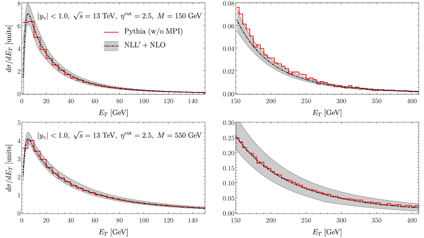
Figure 1: The NLL-prime resumed distributions evaluated from Eq.(38) (black dot-dashed) compared against the result from Pythia partonic distributions (red solid).

Comparing our matched NLL’ result against a simulation using MadGraph Alwall:2014hca +Pythia Sjostrand:2006za ; Sjostrand:2007gs , we find good agreement. The hard process $pp\to\gamma^{*}$ is performed in MadGraph and then showered by Pythia. We use Pythia build-in matrix element (ME) corrections for describing the distribution in the far tail. As discussed in Refs. Sjostrand:2006za ; Sjostrand:2007gs this corresponds up to one additional hard emission from the initial state partons. This is sufficient for our case since we are matching only to NLO corrections in that region. In Figure 1, we show the comparison in the peak region (left) and tail region (right) for the choice $\eta_{\text{cut}}=2.5$.

The error band is estimated by varying all scales by a factor of two and one-half around their canonical values. The total error is calculated by adding in quadrature all variations. Caution is necessary here since the scales choice is implemented through the profile functions in order to transition from one region to the other. That requires that a single profile function will change with any of the scale variations in order to ensure the proper transition without double counting the variations. For example, the global-soft and beam profiles will change accordingly when we consider hard scale variation in order to freeze evolution in the far tail but should remain unchanged for $E_{T}\ll Q$. We collected all the details on the choice of profile functions and scale variation in Appendix D.

In order to compare our analytic result with the partonic distributions in Pythia we turned off the multi-parton interactions and hadronization. The non-perturbative/hadronization effects on the resummed distributions can be studied using the operator definition of the soft and collinear functions Korchemsky:2000kp ; Bauer:2002ie ; Lee:2006fn ; Lee:2007jr . Usually the hadronization effects are included through a convolution of the soft function or the cross section with a model function (which needs to be determined from experiment). The convolution is over the measured observable and thus the model function depends on the observable. The form of the model function is usually determined using the operator product expansion to get the first few moments. This was done for various event and jet-shape observables such as thrust, event-shape angularities, jet mass, groomed-jet mass, $D_{2}$, e.t.c. Hornig:2009vb ; Kang:2013lga ; Kang:2018qra ; Moult:2017okx ; Stewart:2014nna . Ref. Becher:2013iya , studies the non-perturbative effects in transverse momentum dependent (TMD) distributions and jet broadening in $e^{+}e^{-}$ which are most closely related to the measurement presented in this paper.

In contrast, contributions from multi-parton interactions (MPI) are not very well understood theoretically, and a systematic approach for describing these effects has yet to be developed. The subject of MPI and how our formalism can be used to study its effect is discussed in the next section.

3 Multiparton interactions

The origin of MPI is from secondary interactions of the beam remnants through Glauber exchanges. These interactions are known to break factorization in measurements of global observables but cancel in inclusive cross-sections. A variety of MPI sensitive observables are used in experimental studies for understanding the properties of underlying event (UE) but a comparison to the theory is currently impossible. In this paper we propose a prescription to describe MPI contributions to transverse energy with a rapidity cutoff. In experimental measurements of UE common choices for the rapidity cutoff parameter are $\eta_{\text{cut}}=2$ and $\eta_{\text{cut}}=2.5$ (for example, see Refs. Aaboud:2017fwp ; Aad:2016ria ; Chatrchyan:2012tb ; CMS:2016etb ; Aad:2014hia ). Our prescription is based on the following two conjectures:

• Contributions to underlying event from MPI can be modeled by a convolution of a model function with perturbative results,

• The MPI model function is insensitive to hard scale $Q$.

These assumptions lead to the following expression for the transverse energy spectrum including MPI,

$$\frac{d\sigma^{\text{pert+MPI}}}{dE_{T}}=\frac{d\sigma^{\text{pert}}}{dE_{T}}\otimes f_{\text{MPI}}(E_{T},\eta_{\text{cut}})\;,$$ (41)

where $f_{\text{MPI}}(E_{T},\eta_{\text{cut}})$ is the model function that needs to be fitted to the experiment. Similar approach was used in Refs. Stewart:2014nna ; Hoang:2017kmk ; Kang:2018jwa in order to incorporate for contribution from UE to jet substructure observables. We allow the model function to depend on $\eta_{\text{cut}}$ to properly incorporate the change in phase-space for different experiments. The dependence on $\eta_{\text{cut}}$ can give us useful information regarding the pseudo-rapidity distribution of MPI in hadronic collisions.

Note that the second conjecture can be relaxed allowing the model function to vary slowly with the hard scale. Then instead of Eq.(41), the transverse energy spectrum is given by

$$\frac{d\sigma^{\text{pert+MPI}}}{dE_{T}}=\int dQ\;\frac{d\sigma^{\text{pert}}}{dE_{T}dQ}\otimes f_{\text{MPI}}(E_{T},Q,\eta_{\text{cut}})\;,$$ (42)

This approach might be more appropriate in studies over an extended range of $Q$. In this work we consider $Q\in(100,1000)$ GeV and in this region it is sufficient to use the model of Eq.(41). For the parameterizations of the MPI model function we used the half normal distribution,

$$f_{\text{MPI}}(E_{T},\eta_{\text{cut}})=\mathcal{N}\exp\Big{[}-\Big{(}\frac{E_{T}}{\alpha(\eta_{\text{cut}})\sqrt{\pi}}\Big{)}^{2}\Big{]}\Theta(E_{T}),$$ (43)

where $\mathcal{N}=2/(\alpha(\eta_{\text{cut}})\,\pi)$ fixes the normalization of the model function to unity and $\alpha(\eta_{\text{cut}})$ controls the first moment of the model function,

$$\alpha(\eta_{\text{cut}})=\langle E_{T}\rangle_{f}=\int_{0}^{\infty}dE_{T}\,E_{T}\,f_{\text{MPI}}(E_{T},\eta_{\text{cut}}).$$ (44)

If the conjectures above can be shown to be true up to power corrections, within the effective theory, then $\alpha(\eta_{\text{cut}})$ can be written in terms of universal non-perturbative functions such as multiparton distribution functions. Here $\alpha(\eta_{\text{cut}})$ can be fixed directly from experimental measurements using,

$$\alpha(\eta_{\text{cut}})=\langle E_{T}\rangle_{\text{exp.}}-\langle E_{T}\rangle_{\text{pert.}}\,.$$ (45)

Since no experimental data are available for this measurement (see Refs. Aaboud:2017fwp ; Aad:2016ria ; Chatrchyan:2012tb ; CMS:2016etb ; Aad:2014hia for relevant experimental studies) we use Monte Carlo simulation data. We find that in the region $1.5<\eta_{\text{cut}}<3.5$, $\alpha(\eta_{\text{cut}})$ can be well described by a linear fit,

$$\alpha(\eta_{\text{cut}})=A\;\eta_{\text{cut}}\;,$$ (46)

where $A$ is a parameter that describes the mean transverse energy deposited in the central region from MPI, and depends on the hadronic invariant mass, $\sqrt{s}$. Since in this work we are considering only $\sqrt{s}=13$ TeV we treat $A$ as a constant. Fitting to the simulation data, we find $A=22.7$ GeV.

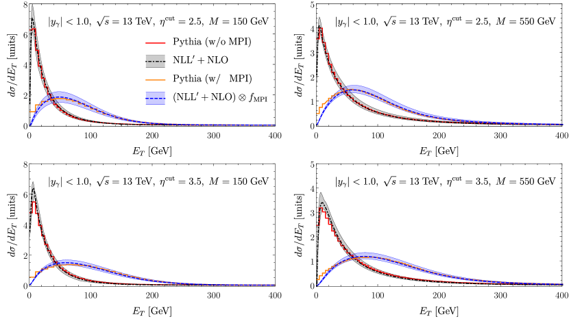
Figure 2: The NLL-prime resumed distributions evaluated from Eq.(38) and convolved with the half Gaussian model function (blue dashed) and the Pythia simulations (ISR+MPI) (orange solid). We also included the purely perturbative result (black dot-dashed) compared against the result from Pythia partonic distributions (MPI-only) (red solid). In each plot all curves are arbitrarily normalized to the same area.

In Figure 2, we illustrate the effect of MPI interactions to measurements of transverse energy within a pseudo-rapidity region, as described by Pythia. Once MPI effects are included, the transverse energy distribution differs significantly from the perturbation calculation. On the other hand, by includingthe contribution in Eq.(41) with the model in Eq.(43) we were able to accurately describe the simulation data.

We emphasize here that the aim of this section is to illustrate that a relatively simple model can describe the contribution of MPI for a large spectrum of the partonic invariant mass. More flexible models can achieve even better agreement, for example one can deviate from the linear fit in Eq.(46) allowing $A$ to depend on $\eta_{\text{cut}}$. Also we could deviate from he functional from of $f_{\text{MPI}}$ of Eq.(43) (see also the work in Ref. Papaefstathiou:2010bw where the dependence of $f_{\text{MPI}}$ on $s$ for fixed $\eta_{\text{cut}}=4.5$ is discussed).

3.1 MPI-insensitive observables

In this section we show how we can use measurements of transverse energy to construct observables independent of MPI. Our proposal depends on the conjunctures above Eq.(41) thus the observables we propose can be used either in order to validate these conjunctures or for phenomenological studies, e.g., one can test the conjectures in Drell-Yan and use them in phenomenological studies of Higgs production.

We define the subtracted moments as follows

$$\Delta E_{T}^{(n)}(Q,Q_{0})\equiv\langle E_{T}^{n}(Q)\rangle-\langle E_{T}^{n}(Q_{0})\rangle$$ (47)

where, $\langle E_{T}^{n}(Q)\rangle$ is the $n^{\text{th}}$ moment at the hard scale $Q$ and is defined by the following

$$\langle E_{T}^{n}(Q)\rangle=\int_{0}^{\infty}dE_{T}\,E_{T}^{n}\,\frac{d\sigma(E_{T},Q)}{dE_{T}}\Big{/}\int_{0}^{\infty}dE_{T}\frac{d\sigma(E_{T},Q)}{dE_{T}}$$ (48)

where $\sigma(E_{T},Q)$ refers to the differential cross section in $E_{T}$ and $Q$. Assuming the MPI contribution can be modeled by a function $f_{\text{MPI}}(E_{T})$ convoluted with the perturbative cross section in Eq. (2.2) we have,

$$\sigma(E_{T},Q)=\int dE_{T}^{\prime}\,f_{\text{MPI}}(E_{T}-E_{T}^{\prime})\theta(E_{T}-E_{T}^{\prime})\sigma^{\text{pert}}(E_{T}^{\prime},Q)$$ (49)

The numerator in Eq. (48) can be written as

$$\int_{0}^{\infty}dE_{T}E_{T}^{n}\int dE_{T}^{\prime}\,f_{\text{MPI}}(E_{T}-E_{T}^{\prime})\theta(E_{T}-E_{T}^{\prime})\sigma^{\text{pert}}(E_{T}^{\prime},Q)\,,$$

$$=\int dE_{T}^{\prime}\,\sigma^{\text{pert}}(E_{T}^{\prime},Q)\int dE_{T}(E_{T}^{\prime}+\omega)^{n}f_{\text{MPI}}(\omega)\theta(\omega)\,,$$

$$=\sum_{k=0}^{n}{}_{n}C_{k}\int dE_{T}^{\prime}\,(E_{T}^{\prime})^{k}\sigma^{\text{pert}}(E_{T}^{\prime},Q)\times\int d\omega\;\omega^{n-k}f_{\text{MPI}}(\omega)\theta(\omega)$$ (50)

where in the second line we changed the integration variable to $\omega=E_{T}-E_{T}^{\prime}$ and ${}_{n}C_{k}$ are the binomial coefficients. With this, Eq. (48) can be written as

$$\langle E_{T}^{n}(Q)\rangle=\sum_{k=0}^{n}{}_{n}C_{k}\,\langle E_{T}^{k}(Q)\rangle_{\text{pert}}\times\langle E_{T}^{n-k}\rangle_{\text{MPI}}$$ (51)

where the perturbative average $\langle\cdots\rangle_{\text{pert}}$ and MPI average $\langle\cdots\rangle_{\text{MPI}}$ are defined by Eq. (48) with the replacement of the cross section by perturbative cross section $\sigma_{\text{pert}}(E_{T},Q)$ and by the MPI model function $f_{\text{MPI}}(E_{T})$ respectively. Applying Eq. (51) in Eq.47 we get

$$\Delta E_{T}^{(n)}(Q,Q_{0}) =\sum_{k=1}^{n}{}_{n}C_{k}\,\left(\langle E_{T}^{k}(Q)\rangle_{\text{pert}}-\langle E_{T}^{k}(Q_{0})\rangle_{\text{pert}}\right)\times\langle E_{T}^{n-k}\rangle_{\text{MPI}}\,,$$

$$=\sum_{k=1}^{n}{}_{n}C_{k}\,\Delta E_{T,\text{pert}}^{(k)}\,\times\langle E_{T}^{n-k}\rangle_{\text{MPI}}$$ (52)

where $\Delta E_{T,\text{pert}}^{(k)}$ is defined in similar way to Eq. (47) in terms of the perturbative cross section. By taking the difference at different values of $Q$, the first term at $k=0$, which is $\langle E_{T}^{n}\rangle_{\text{MPI}}$, cancels. Thus for the first few values of $n$ we have,

$$\Delta E_{T}^{(1)} =\Delta E_{T,\text{pert}}^{(1)}\,,$$

$$\Delta E_{T}^{(2)} =2\Delta E_{T,\text{pert}}^{(2)}+\Delta E_{T,\text{pert}}^{(1)}\,\langle E_{T}\rangle_{\text{MPI}}\,,$$

$$\Delta E_{T}^{(3)} =3\Delta E_{T,\text{pert}}^{(3)}+3\Delta E_{T,\text{pert}}^{(2)}\,\langle E_{T}\rangle_{\text{MPI}}+\Delta E_{T,\text{pert}}^{(1)}\,\langle E_{T}^{2}\rangle_{\text{MPI}}$$ (53)

Therefore, at $n=1$ the MPI contribution precisely cancels and the difference can be predicted by purely perturbative results. We refer to $\Delta E_{T}\equiv\Delta E_{T}^{(1)}$ as the subtracted transverse energy. The difference of higher moments includes MPI contributions that can be used to determine parameters of MPI models. Note that the results in Eq. (3.1) are obtained from the two conjectures above Eq.(41) but are independent of the model function, $f_{\text{MPI}}$.

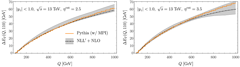
Figure 3: The observabel $\Delta E_{T}(Q,Q_{0})$ for $Q_{0}=110$ GeV for two different values of the rapidity cutoff parameter $\eta_{\text{cut}}=2.5$ (left) and $\eta_{\text{cut}}=3.5$ (right)

We demonstrate the cancelation of the MPI contribution in $\Delta E_{T}$ using Pythia simulation in Figure 3. We are comparing the observable $\Delta E_{T}(Q,110\text{ GeV})$ evaluated with the default MPI model of Pythia and the purely perturbative result. The uncertainty here is evaluated by using the maximum and minimum values of the error bands from the perturbative results. It is clear that, within the uncertainty, the observable $\Delta E_{T}$ is independent of the MPI contributions, as implemented in Pythia, for that range of the hard scale. In Figure 3 shows this for the cases $\eta_{\text{cut}}=2.5$ and $\eta_{\text{cut}}=3.5$.

3.2 Generalization to other observables

The approach of subtracting the mean at different hard scales to obtain MPI-insensitive measurements can be implemented in other observables as well. This is true for additive observables for which the contributions from MPI can be achieved through a convolution. A characteristic example of this is the beam thrust Stewart:2009yx ; Stewart:2010pd ; Berger:2010xi ; Aad:2016ria , $B$, defined as,

$$B=\sum_{i\in X}p_{T}^{(i)}\exp(-{\eta^{(i)}}).$$ (54)

The corresponding subtracted observable is

$$\Delta B(Q,Q_{0})\equiv\langle B(Q)\rangle-\langle B(Q_{0})\rangle.$$ (55)

In Figure 4 we demonstrate that $\Delta B(Q,Q_{0})$ is also insensitive to the MPI contributions for a large range of the virtual photon’s invariant mass. An obvious advantage of using beam thrust is that the contribution of each particle is weighted by $\exp(-\eta)$ and thus contribution from particles in the forward region, close to the rapidity boundary, is exponentially suppressed. Therefore the measurement is insensitive to the rapidity cutoff . On the other hand this means that we cannot use beam thrust as our observable if we aim to study the pseudo-rapidity dependence of MPI through the model function $f_{\text{MPI}}$.

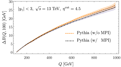
Figure 4: The observable $\Delta B(Q,Q_{0})$ (subtracted beam thrust) for $Q_{0}=100$ GeV and $\eta_{\text{cut}}=4.5$. The uncertainty bands correspond to statistical uncertainty due to finite sample data.

4 Conclusion

In this paper we demonstrated an effective field theory approach for calculating the transverse energy spectrum when a rapidity cutoff is imposed. In contrast to Ref. Hornig:2017pud , in this work we use dynamical (profile) scales in order to interpolate between our result from the small transverse energy region (region II) to large values of transverse energy (region I). Finally we used a subtraction scheme to match onto the fixed order result of the full theory (QCD) at $E_{T}\sim Q$. Although the cross section in the far tail region where $E_{T}\sim Q$ is highly suppressed compared to regions I and II, it is important to know the spectrum in all ranges of $E_{T}$ since the far tail region gives significant contributions when we calculate moments of the transverse energy.

As an example we choose to study the process $pp\to\gamma(\to\ell^{+}\ell^{-})+X$ away from the $Z$-pole region. Comparing our results with Pythia (ISR only) simulations we find excellent agreement. We then proceed to introduce a prescription to include the effect of multiparton interactions (MPI). The prescription we propose, which is based on the conjectures above Eq.(41), is to simply convolve the perturbative spectrum with a model function. The model function should not depend on the hard process but could have small variations with the change of the hard scale in the process. Comparing our result with Pythia (ISR+MPI) we find that for the range 100-1000 GeV of the photon’s invariant mass the MPI model function has little or no hard scale dependence.

Assuming independence of the model function on the hard scale of the problem we introduce an observable, which is independent of MPI effects. This observable we are considering is the subtracted first moment of the transverse energy at two different scales. We compare our purely perturbative calculations of this observable against Pythia (ISR+MPI) and we show that the two agree very well.

Although in this paper we considering only transverse energy measurements, in the last section we discuss generalizations of this MPI insensitive observable to other event shapes, such as beam thrust and transverse thrust. An advantage of using transverse energy as a probe to the MPI effects is that we have strong sensitivity to the rapidity cutoff parameter, $\eta_{\text{cut}}$. Measurements at different values of $\eta_{\text{cut}}$ can give an insight into the pseudo-rapidity dependence of MPI.

The independence of the MPI to the hard process using Monte Carlo simulations was also investigated in Ref. Papaefstathiou:2010bw in Higgs, $Z$, and $W^{\pm}$ production processes implemented in Herwig++ Bahr:2008pv . A future application of our work is to evaluate the Higgs or $Z$/$W^{\pm}$ transverse energy spectrum, using the prescription and model function for MPI we propose in this paper, and compare with results from Monte Carlo simulations.

Appendix A The beam function matching for region I

We evaluate the bare global beam function $\mathcal{O}(\alpha_{s})$ terms using Eq.(25) and (26) from Ref. Ritzmann:2014mka ,

$$\mathcal{B}^{\text{ G (1,b)}}_{q/q}(x,E_{T};\mu,\nu)=\frac{\alpha_{s}C_{F}}{\pi}\frac{\exp(\epsilon\gamma_{E})}{\Gamma(1-\epsilon)}\Big{(}\frac{\nu}{p^{-}}\Big{)}^{\eta}\frac{1}{\mu}\Big{(}\frac{\mu}{E_{T}}\Big{)}^{1+2\epsilon}\Big{[}\frac{1+x^{2}}{(1-x)^{1+\eta}}-\epsilon(1-x)^{1-\eta}\Big{]}.$$ (56)

Expanding first in $\eta$ and then in $\epsilon$ we have,

$$\mathcal{B}^{\text{ G (1,b)}}_{q/q}(x,E_{T};\mu,\nu)=\frac{\alpha_{s}C_{F}}{\pi}\Big{\{}-\frac{1}{\eta}\Big{[}-\frac{1}{\epsilon}\delta(E_{T})+2\mathcal{L}_{0}(E_{T},\mu)\Big{]}\delta(1-x)\\ +\frac{1}{\epsilon}\Big{[}\ln\Big{(}\frac{\nu}{p^{-}}\Big{)}\delta(1-x)-\frac{1}{2}\bar{P}_{q/q}(x)\Big{]}\delta(E_{T})+\mathcal{L}_{0}(E_{T},\mu)\Big{[}\bar{P}_{q/q}(x)-2\ln\Big{(}\frac{\nu}{p^{-}}\Big{)}\delta(1-x)\Big{]}\\ +c_{q/q}(x)\delta(E_{T})\Big{\}},$$ (57)

where

$$c_{q/q}(x)=\frac{1-x}{2},$$ (58)

and

$$\bar{P}_{q/q}(x)=\frac{1+x^{2}}{(1-x)_{+}}-\frac{3}{2}\delta(1-x)=P_{q/q}(x)-\bar{\gamma}_{q}\;\delta(1-x),$$ (59)

where $P_{i/j}(x)$ are the QCD splitting kernels Altarelli:1977zs ; PhysRevD.9.980 and $\bar{\gamma}_{q}=3/2$. The divergent $P_{q/q}(x)/\epsilon$ term cancels during the matching with the collinear parton distribution functions (PDFs) and therefore should not be included in the renormalization kernel. Thus in the $\overline{\text{MS}}$ scheme this yields,

$$\mathcal{I}^{\text{ G (NLO)}}_{q/q}(x,E_{T},p^{-})=\delta(E_{T})\delta(1-x)+\frac{\alpha_{s}C_{F}}{\pi}\Big{\{}\mathcal{L}_{0}(E_{T},\mu)\Big{[}\bar{P}_{q/q}(x)-2\ln\Big{(}\frac{\nu}{p^{-}}\Big{)}\delta(1-x)\Big{]}\\ +c_{q/q}(x)\delta(E_{T})\Big{\}},$$ (60)

and the corresponding renormalization function

$$Z_{q/q}^{\text{B,G (1)}}(E_{T},p^{-})=\delta(E_{T})+\frac{\alpha_{s}C_{F}}{\pi}\Big{\{}-\frac{1}{\eta}\Big{[}2\mathcal{L}_{0}(E_{T},\mu)-\frac{1}{\epsilon}\delta(E_{T})\Big{]}+\frac{1}{\epsilon}\Big{[}\ln\Big{(}\frac{\nu}{p^{-}}\Big{)}+\frac{1}{2}\bar{\gamma}_{q}\Big{]}\delta(E_{T})\Big{\}},$$ (61)

where we omitted the rapidity and virtuality scale the arguments for simplicity of notation. To evaluate the off-diagonal element $\mathcal{I}_{q/g}^{\text{ G}}$ we start with the corresponding partonic beam function given in Eq.(26) of Ref. Ritzmann:2014mka ,

$$\mathcal{B}_{q/g}^{\text{ G (1,b)}}(x,E_{T},p^{-};\mu,\nu)=\frac{\alpha_{s}T_{F}}{\pi}\frac{e^{\epsilon\gamma_{E}}}{\Gamma(2-\epsilon)}\Big{(}\frac{\nu}{p^{-}}\Big{)}^{\eta}\frac{1}{\mu}\Big{(}\frac{\mu}{E_{T}}\Big{)}^{1+2\epsilon}(1-x)^{-\eta}\Big{[}P_{q/g}(x)-\epsilon\Big{]}.$$ (62)

where

$$P_{q/g}(x)=x^{2}+(1-x)^{2}$$ (63)

Expanding first in $\eta$ and then in $\epsilon$ we have,

$$\mathcal{B}_{q/g}^{\text{ G (1,b)}}(x,E_{T},p^{-};\mu,\nu)=\frac{\alpha_{s}T_{F}}{\pi}\Big{\{}-\frac{1}{2\epsilon}P_{q/g}(x)+\mathcal{L}_{0}(E_{T},\mu)P_{q/g}(x)+c_{q/g}(x)\delta(E_{T})\Big{\}},$$ (64)

where

$$c_{q/g}(x)=x(1-x).$$ (65)

Except the term $P_{q/g}(x)/\epsilon$ which cancels during the matching there is no other divergent term. Thus the contribution from the off-diagonal element at this order does not contribute to the renormalization function or the corresponding anomalous dimension. Thus the matching coefficient is,

$$\mathcal{I}_{q/g}^{\text{ G (NLO)}}=\frac{\alpha_{s}T_{F}}{\pi}\Big{\{}\mathcal{L}_{0}(E_{T},\mu)P_{q/g}(x)+c_{q/g}(x)\delta(E_{T})\Big{\}}.$$ (66)

The rapidity and virtuality anomalous dimensions, $\gamma_{\nu}$ and $\gamma_{\mu}$ respectively are evaluated using the following,

$$\gamma_{\nu,q}^{\text{B,G}}(E_{T};\mu) =-(Z^{\text{B,G}}_{q/q})^{-1}\otimes\frac{d}{d\ln(\nu)}Z^{\text{B,G}}_{q/q},$$ (67)

$$\gamma_{\mu,q}^{\text{B,G}}(p^{-};\mu,\nu)\delta(E_{T}) =-(Z^{\text{B,G}}_{q/q})^{-1}\otimes\frac{d}{d\ln(\mu)}Z^{\text{B,G}}_{q/q},$$ (68)

and thus we have

$$\gamma_{\nu,q}^{\text{B,G}}(E_{T};\mu) =-\frac{2\alpha_{s}(\mu)C_{F}}{\pi}\mathcal{L}_{0}(E_{T},\mu),$$ (69)

$$\gamma_{\mu,q}^{\text{B,G}}(p^{-};\mu,\nu) =\frac{\alpha_{s}(\mu)C_{F}}{\pi}\Big{[}2\ln\Big{(}\frac{\nu}{p^{-}}\Big{)}+\bar{\gamma}_{q}\Big{]}.$$ (70)

Appendix B Merging fixed order

Here we perform an explicit calculation to show that the product $S_{n}\otimes\mathcal{B}^{\text{ II}}_{a/P}$ reduces to $\mathcal{B}^{\text{ G}}_{a/P}$ in the large transverse energy limit, $E_{T}\gg Qr$. To this end, we work with the partonic-level functions, $\mathcal{B}^{\text{ G}}_{q/i}$ in Eq. (6) and the combination of soft-collinear and beam function $S_{n}\otimes\mathcal{B}^{\text{ II}}_{q/i}$ in Eq.(2.2) where $i=q,g$. At $\mathcal{O}(\alpha_{s}^{1})$ we have

$$S_{n}(E_{T},r;\mu,\nu)\otimes\mathcal{B}^{\text{ II}}_{q/i}(x,E_{T},r;\mu)=\delta_{qi}\delta(E_{T})\delta(1-x)\\[3.0pt] +S^{(1)}_{n}(E_{T},r;\mu,\nu)\delta_{qi}\delta(1-x)+\mathcal{I}_{q/i}^{\text{ II}\;(1)}(x,E_{T},r;\mu)+\mathcal{O}(\alpha_{s}^{2}),$$ (71)

and

$$\mathcal{B}^{\text{ G}}_{q/P}(x,E_{T};\mu,\nu)=\delta_{qi}\delta(E_{T})\delta(1-x)+\mathcal{I}_{q/i}^{\text{ G}\;(1)}(x,E_{T};\mu,\nu)+\mathcal{O}(\alpha_{s}^{2}),$$ (72)

therefore we need to show

$$\Big{[}S^{(1)}_{n}(E_{T},r;\mu,\nu)\delta_{qi}\delta(1-x)+\mathcal{I}_{q/i}^{\text{ II}\;(1)}(x,E_{T},r;\mu)\Big{]}\xrightarrow{E_{T}\gg Qr}\;\mathcal{I}_{q/i}^{\text{ G}\;(1)}(x,E_{T};\mu,\nu)+\text{p.c.}$$ (73)

This task becomes much easier if we work with cumulant bare functions defined

$$F(p_{T}^{\mathrm{cut}})=\int_{0}^{p_{T}^{\mathrm{cut}}}F(E_{T})$$ (74)

where the cumulant of the one-loop beam function in Eq. (6) is given by integrating Eq.(56),

$$\mathcal{I}_{q/q}^{\text{ G}\;(1)}(x,p_{T}^{\mathrm{cut}})=\frac{\alpha_{s}C_{F}}{\pi}\frac{e^{\epsilon\gamma_{E}}}{\Gamma(1-\epsilon)}\Big{(}\frac{\nu}{p^{-}}\Big{)}^{\eta}\Big{[}\frac{1+x^{2}}{(1-x)^{1+\eta}}-\epsilon(1-x)^{1-\eta}\Big{]}\frac{-1}{2\epsilon}\Big{(}\frac{\mu}{p_{T}^{\mathrm{cut}}}\Big{)}^{2\epsilon}.$$ (75)

The one-loop cumulant soft-collinear function is given integrating Eq.(2.12) of Ref.Hornig:2017pud

$$S^{(1)}_{n}(p_{T}^{\mathrm{cut}},r)=-\frac{\alpha_{s}C_{F}}{2\pi}\frac{4e^{\epsilon\gamma_{E}}}{\Gamma(1-\epsilon)}\frac{1}{\eta}\Big{(}\frac{\nu r}{\mu}\Big{)}^{\eta}\frac{-1}{2\epsilon+\eta}\Big{(}\frac{\mu}{p_{T}^{\mathrm{cut}}}\Big{)}^{2\epsilon+\eta}\,,$$ (76)

and the one-loop cumulant beam function consists of in-jet, out-of-jet, the zero-bin contributions, given by integrating Eqs.(B.1), (B.10), and (B.13) of Ref. Hornig:2017pud respectively,

$$\mathcal{I}_{q/q}^{\text{ II}\;(1)}(x,p_{T}^{\mathrm{cut}},r)=\mathcal{I}_{q/q}^{(1)}(x,r)+(\Delta B^{\text{out}}_{q/q}(x,p_{T}^{\mathrm{cut}},r)-\Delta B^{\text{zero}}_{q/q}(x,p_{T}^{\mathrm{cut}},r))\,,$$ (77)

where

$$\mathcal{I}_{q/q}^{(1)}(x,r) =-\frac{\alpha_{s}C_{F}}{2\pi}\frac{e^{\epsilon\gamma_{E}}x^{2\epsilon}}{\epsilon\Gamma(1-\epsilon)}\Big{(}\frac{\mu}{p^{-}r}\Big{)}^{2\epsilon}\Big{[}\frac{1+x^{2}}{(1-x)^{1+2\epsilon}}-\epsilon(1-x)^{1-2\epsilon}\Big{]}\,,$$

$$\Delta B^{\text{out}}_{q/q}(x,p_{T}^{\mathrm{cut}},r) =\frac{\alpha_{s}C_{F}}{2\pi}\frac{e^{\epsilon\gamma_{E}}}{\epsilon\Gamma(1-\epsilon)}\Big{(}\frac{\nu}{p^{-}}\Big{)}^{\eta}\Big{[}\frac{1+x^{2}}{(1-x)^{1+\eta}}-\epsilon(1-x)^{1-\eta}\Big{]}$$

$$\quad\times\theta(x-x_{0})\Big{[}\Big{(}\frac{\mu}{p^{-}r}\frac{x}{1-x}\Big{)}^{2\epsilon}-\Big{(}\frac{\mu}{p_{T}^{\mathrm{cut}}}\Big{)}^{2\epsilon}\Big{]},$$

$$\Delta B^{\text{zero}}_{q/q}(x,p_{T}^{\mathrm{cut}},r) =\delta(1-x)\,S^{(1)}_{n}\,,$$ (78)

where $x_{0}=[1+p_{T}^{\mathrm{cut}}/(p^{-}r)]^{-1}$. Note that the zero-bin contribution on the last line is precisely cancelled against the soft-collinear function in Eq. (76).

$$S^{(1)}_{n}(p_{T}^{\mathrm{cut}},r)\delta(1-x) +\mathcal{I}_{q/q}^{\text{ II}\;(1)}(x,p_{T}^{\mathrm{cut}},r)$$

$$=\mathcal{I}_{q/q}^{(1)}(x,r)+\Delta B^{\text{out}}_{q/q}(x,p_{T}^{\mathrm{cut}},r)$$

$$=\mathcal{I}_{q/q}^{\text{ G}\;(1)}(x,p_{T}^{\mathrm{cut}})+\Delta B^{\text{out}}_{q/q}(x,p_{T}^{\mathrm{cut}},r)\Big{|}_{\theta(x-x_{0})\to\theta(x-x_{0})-\theta(x)}\;.$$ (79)

In the last step, we use the identify:

$$\Delta B^{\text{out}}_{q/q}(x,p_{T}^{\mathrm{cut}},r)=\theta(x-x_{0})\Big{[}-\mathcal{I}_{q/q}^{(1)}(x,r)+\mathcal{I}_{q/q}^{\text{ G}\;(1)}(x,p_{T}^{\mathrm{cut}})\Big{]}+\mathcal{O}(\eta)\;.$$ (80)

Note that the second term on last line is simply power corrections in the limit $p_{T}^{\mathrm{cut}}\ll p^{-}r$:

$$\theta(x-x_{0})-\theta(x)\to-\Big{(}\frac{p^{-}r}{p_{T}^{\mathrm{cut}}}\Big{)}\delta(x)+O\Big{[}\Big{(}\frac{p^{-}r}{p_{T}^{\mathrm{cut}}}\Big{)}^{2}\Big{]}\;.$$ (81)

This shows the diagonal element (i.e., $i=q$) of Eq.(73) up to power corrections.

The gluon channel is similar but simpler. The gluon channel contribution in Eq. (6) can be found integrating Eq.(62) and setting $\eta\to 0$

$$\mathcal{I}_{q/g}^{\text{ G}\;(1)}(x,p_{T}^{\mathrm{cut}})=-\frac{\alpha_{s}T_{F}}{2\pi}\frac{e^{\epsilon\gamma_{E}}}{\epsilon\;\Gamma(2-\epsilon)}\Big{[}P_{qg}(x)-\epsilon\Big{]}\Big{(}\frac{\mu}{p_{T}^{\mathrm{cut}}}\Big{)}^{2\epsilon}\;.$$ (82)

There is no zero-bin contribution in the gluon channel thus using Eqs.(B.4) and (B.18) of Ref. Hornig:2017pud

$$\mathcal{I}_{q/g}^{\text{ II}\;(1)}(x,p_{T}^{\mathrm{cut}},r)=\mathcal{I}_{q/g}^{(1)}(x,r)+\Delta B^{\text{out}}_{q/g}(x,p_{T}^{\mathrm{cut}},r)\,,$$ (83)

where

$$\mathcal{I}_{q/g}^{(1)}(x,r) =-\frac{\alpha_{s}T_{F}}{2\pi}\Big{(}\frac{1}{\epsilon}+1\Big{)}\Big{(}\frac{x}{1-x}\Big{)}^{2\epsilon}\Big{(}\frac{\mu}{p^{-}r}\Big{)}^{2\epsilon}\left[P_{qg}(x)-\epsilon\right]\,,$$

$$\Delta B^{\text{out}}_{q/g}(x,p_{T}^{\mathrm{cut}},r) =\frac{\alpha_{s}T_{F}}{\pi}\frac{1}{2\epsilon(1-\epsilon)}\left[P_{qg}(x)-\epsilon\right]\theta(x-x_{0})\Big{[}\Big{(}\frac{\mu}{p^{-}r}\frac{x}{1-x}\Big{)}^{2\epsilon}-\Big{(}\frac{\mu}{p_{T}^{\mathrm{cut}}}\Big{)}^{2\epsilon}\Big{]}\;.$$ (84)

By comparing Eq. (82) to Eq. (83), we find

$$\Delta B^{\text{out}}_{q/g}(x,p_{T}^{\mathrm{cut}},r)=\theta(x-x_{0})\Big{[}\mathcal{I}_{q/g}^{\text{ G}\;(1)}(x,p_{T}^{\mathrm{cut}})-\mathcal{I}_{q/g}^{(1)}(x,r)\Big{]}+\mathcal{O}(\epsilon)\;,$$ (85)

and we have

$$\mathcal{I}_{q/g}^{\text{ II}\;(1)}(x,p_{T}^{\mathrm{cut}},r)=\mathcal{I}_{q/g}^{\text{ G}\;(1)}(x,p_{T}^{\mathrm{cut}})+\Delta B^{\text{out}}_{q/g}(x,p_{T}^{\mathrm{cut}},r)\Big{|}_{\theta(x-x_{0})\to\theta(x-x_{0})-\theta(x)}\;.$$ (86)

As in Eq. (B), the second term on RHS is the power correction.

Appendix C Evolution and resummation

In this appendix we give the details for the solutions of the renormalization group and rapidity renormalization group equations. This section is divided into two subsections. In Section C.1 we discuss the virtuality renormalization group equations and the solutions of those equations and in Section C.2 the rapidity renormalization group evolution is described. All elements of factorization (hard, soft, soft-collinear, and beam) satisfy renormalization group equations, in contrast, only transverse energy dependent quantities have rapidity RGE.

C.1 Renormalization group evolution

The RGEs we encounter in this work belong to the same category of what was referred to in Ref. Hornig:2017pud as unmeasured evolution equations. In this paper we do not discuss the evolution of measured quantities and therefore such a distinction is redundant. Also for the processes we are considering the hard and soft function have trivial color structure and therefore we do not address the complications that appear when one considers multi-jet processes in hadronic collisions. The RGEs we consider have the following form,

$$\frac{d}{d\ln\mu}F(\mu)=\gamma_{\mu}^{F}(\mu,\alpha_{s})F(\mu)=\Big{[}\Gamma^{F}_{\mu}[\alpha_{S}]\ln\Big{(}\frac{\mu^{2}}{m^{2}_{F}}\Big{)}+\Delta\gamma^{F}_{\mu}[\alpha_{S}]\Big{]}F(\mu),$$ (87)

where $\gamma_{\mu}^{F}$ is the virtuality anomalous dimension. We refer to the first term in the square brackets as the cusp part since $\Gamma^{F}_{\mu}[\alpha_{s}]$ is proportional to the cusp anomalous dimension, and the second term, $\Delta\gamma^{F}_{\mu}[\alpha_{S}]$, as the non-cusp part. Both the cusp and the non-cusp terms have an expansion in the strong coupling. For the cusp term we have,

$$\Gamma_{F}[\alpha_{s}]=(\Gamma_{F}^{0}/\Gamma_{\text{cusp}}^{0})\Gamma_{\text{cusp}}=(\Gamma_{F}^{0}/\Gamma_{\text{cusp}}^{0})\sum_{n=0}^{\infty}\left(\frac{\alpha_{s}}{4\pi}\right)^{1+n}\Gamma_{\text{cusp}}^{n},$$ (88)

and similarly the non-cusp part is given by,

$$\gamma_{F}[\alpha_{s}]=\sum_{n=0}^{\infty}\left(\frac{\alpha_{s}}{4\pi}\right)^{1+n}\gamma_{F}^{n},$$ (89)

The solution to the RGE in Eq.(87) is

$$F(\mu) =\mathcal{U}_{F}(\mu,\mu_{0})F(\mu_{0})\,, \mathcal{U}_{F}(\mu,\mu_{0})=\exp\left(K_{F}(\mu,\mu_{0})\right)\left(\frac{\mu_{0}}{m_{F}}\right)^{\omega_{F}(\mu,\mu_{0})},$$ (90)

with

$$K_{F}(\mu,\mu_{0}) =2\int_{\alpha(\mu_{0})}^{\alpha(\mu)}\frac{d\alpha}{\beta(\alpha)}\Gamma_{F}(\alpha)\int_{\alpha(\mu_{0})}^{\alpha}\frac{d\alpha^{\prime}}{\beta(\alpha^{\prime})}+\int_{\alpha(\mu_{0})}^{\alpha(\mu)}\frac{d\alpha}{\beta(\alpha)}\gamma_{F}(\alpha),$$ (91)

$$\omega_{F}(\mu,\mu_{0}) =2\int_{\alpha(\mu_{0})}^{\alpha(\mu)}\frac{d\alpha}{\beta(\alpha)}\Gamma_{F}(\alpha).$$ (92)

Since in this work we are interested only in the NLL and NLL’ result we may keep only the first two terms in the perturbative expansion of the cusp part (i.e., $\Gamma_{0}^{F}$, $\Gamma^{0}_{\text{cusp}}$, and $\Gamma^{1}_{\text{cusp}}$) and only the first term form the non-cusp part ($\gamma_{F}^{0}$). Performing this expansion we get,

$$K_{F}(\mu,\mu_{0}) =-\frac{\gamma_{F}^{0}}{2\beta_{0}}\ln r-\frac{2\pi\Gamma_{F}^{0}}{(\beta_{0})^{2}}\Big{[}\frac{r-1+r\ln r}{\alpha_{s}(\mu)}+\left(\frac{\Gamma^{1}_{\text{cusp}}}{\Gamma^{0}_{\text{cusp}}}-\frac{\beta_{1}}{\beta_{0}}\right)\frac{1-r+\ln r}{4\pi}+\frac{\beta_{1}}{8\pi\beta_{0}}\ln^{2}r\Big{]},$$ (93)

$$\omega_{F}(\mu,\mu_{0}) =-\frac{\Gamma_{F}^{0}}{\beta_{0}}\Big{[}\ln r+\left(\frac{\Gamma^{1}_{\text{cusp}}}{\Gamma^{0}_{\text{cusp}}}-\frac{\beta_{1}}{\beta_{0}}\right)\frac{\alpha_{s}(\mu_{0})}{4\pi}(r-1)\Big{]},$$ (94)

where $r=\alpha(\mu)/\alpha(\mu_{0})$ and $\beta_{n}$ are the coefficients of the QCD $\beta$-function,

$$\beta(\alpha_{s})=\mu\frac{d\alpha_{s}}{d\mu}=-2\alpha_{s}\sum_{n=0}^{\infty}\left(\frac{\alpha_{s}}{4\pi}\right)^{1+n}\beta_{n}\;.$$ (95)

Table 1 the expressions for all ingredients necessary to perform the evolution of any function that appears in the factorization theorems we considered in this paper are given in.

Function	$H_{a\bar{a}}$	$S_{s}^{a\bar{a}}$	$S_{n}^{a}$	$\mathcal{B}_{a/P}^{\text{G}}$	$\mathcal{B}_{a/P}^{\text{II}}$
$\Gamma_{F}^{0}$	$-4(C_{a}+C_{\bar{a}})$	$4(C_{a}+C_{\bar{a}})$	$-4C_{a}$	0	$4C_{a}$
$\gamma_{F}^{0}$	$-4\bar{\gamma}_{a}(C_{a}+C_{\bar{a}})$	0	0	$4\pi\gamma_{\mu,a}^{\text{B, G}}/\alpha_{s}$	$4C_{a}\bar{\gamma}_{a}$
$m_{F}$	$Q$	$\nu_{ss}$	$\nu_{sc}r$	n.a.	$p^{-}r$
$\xi_{F}$	n.a.	$4(C_{a}+C_{\bar{a}})$	$-4C_{a}$	$-4C_{a}$	n.a.
$\Delta\gamma_{\nu}^{F}$	n.a.	$\mathcal{O}(\alpha_{s})$	$\mathcal{O}(\alpha_{s})$	$\mathcal{O}(\alpha_{s})$	n.a.

Table 1: Evolution table: $\bar{\gamma}_{q}=3/2$ and $\gamma_{\mu,a}^{\text{B, G}}=(\alpha_{s}(\mu)C_{F}/\pi)\Big{(}2\ln(\nu/p^{-})+\bar{\gamma}_{q}\Big{)}$.

C.2 Rapidity renormalization group evolution

In this section we summarize the solution for the rapidity renormalization group equations for the global soft, $S_{s}$, soft-collinear, $S_{n}$, and global beam, $\mathcal{B}_{a/P}^{\text{G}}$ functions. Even though the unmeasured beam function of region II has transverse energy dependence, it does not have rapidity divergences and thus does not acquire rapidity scale dependence. The RRG equation for transverse energy measurements of the function $F(E_{T})\in\{S_{s},S_{n},\mathcal{B}^{\text{G}}_{a/P}\}$ takes the following form,

$$\frac{d}{d\ln\nu}F(E_{T},\mu,\nu)=\int dE_{T}^{\prime}\;\gamma_{\nu}^{F}(E_{T}-E_{T}^{\prime},\mu)F(E_{T}^{\prime},\mu,\nu)\equiv\gamma_{\nu}^{F}\otimes F(E_{T},\mu,\nu),$$ (96)

where

$$\gamma_{\nu}^{F}(E_{T},\mu)=2\Gamma_{\nu}^{F}[\alpha_{s}]\mathcal{L}_{0}(E_{T},\mu)+\Delta\gamma_{\nu}^{F}[\alpha_{s}].$$ (97)

The solution of this equations is

$$F(E_{T},\mu,\nu)=\int dE_{T}\;\mathcal{V}_{F}(E_{T}-E_{T}^{\prime},\mu,\nu,\nu_{0})F(E_{T}^{\prime},\mu,\nu_{0}),$$ (98)

where

$$\mathcal{V}_{F}(E,\mu,\nu,\nu_{0})=\frac{e^{\kappa_{F}(\mu,\nu,\nu_{0})}(e^{\gamma_{E}}\mu)^{-\eta_{F}(\mu,\nu,\nu_{0})}}{\Gamma(\eta_{F}(\mu,\nu,\nu_{0}))}\Big{[}\frac{1}{E^{1-\eta_{F}(\mu,\nu,\nu_{0})}}\Big{]}_{+},$$ (99)

and

$$\eta_{F}(\mu,\nu,\nu_{0}) =2\Gamma_{\nu}^{F}[\alpha]\ln\left(\frac{\nu}{\nu_{0}}\right), \kappa_{F}(\mu,\nu,\nu_{0}) =\Delta\gamma_{\nu}^{F}[\alpha]\ln\left(\frac{\nu}{\nu_{0}}\right),$$ (100)

where $\nu_{0}$ is the characteristic scale (for each function) from which we start the evolution. This scale is chosen such that rapidity logarithms are minimized. For the global-soft, soft-collinear, and beam functions these scales are given in Table 1. The first term in the rapidity anomalous dimension in Eq.(97) is proportional to the cusp anomalous dimension and the proportionality constant we denote with $\xi_{F}$, ($\Gamma_{\nu}^{F}=\xi_{F}\Gamma_{\text{cusp}}$). We define the the plus-distribution in Eq. (99) through its inverse Laplace transform,

$$\Big{[}\frac{1}{E^{1-\alpha}}\Big{]}_{+}={\cal L}^{-1}\Big{[}s^{\alpha}\,\Gamma[-\alpha]\Big{]}\;.$$

Appendix D Profile functions and scale variation

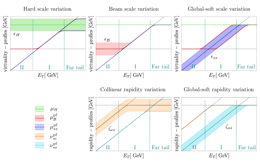
Figure 5: Illustration of the profile scales and how each of the four profile functions changes with the five scale variations. For improving readability we use log-log plots.

In this section we give the details on the choice of profile functions and how scale variation is performed. There are four profile functions. They assist either for the transition from region I to region II or for turning off evolution in the far tail (in order to match onto the fixed order result). The asymptotic behavior in all regions for all profile functions is collected in Eqs.(2.3) and (2.4). The relations in Eq.(2.3) need to be always satisfied in order to reproduce the correct result when transitioning from region II to region I. That is, for example, when we vary $\mu_{ss}$ (in order to explore uncertainty due to scale variation), $\mu_{\mathcal{B}}^{\text{pf}}$ should be varied accordingly.

There are five scale variations that we need to consider: the hard scale, $\mu_{H}$, which extends to all three regions (I, II, and far tail), the global soft scale, $\mu_{ss}$, which extends only to region I and II, the beam scale, $\mu_{\mathcal{B}}^{\text{II}}$, which only applies in region II, the global soft rapidity scale, $\nu_{ss}$, for both regions I and II, and finally the collinear rapidity scale which corresponds to $\nu_{sc}$ in region II, and to $\nu_{\mathcal{B}}$ in region I. In practice we will control these variations through five corresponding parameters, $\epsilon_{H}$, $\epsilon_{ss}$, $\epsilon_{\mathcal{B}}$, $\zeta_{ss}$, and $\zeta_{cs}$ ($=+1,-1,0$). The four profile functions and the hard scale are then defined as follows.

$$\mu_{H}(M;\epsilon_{H})= (2)^{\epsilon_{H}}M$$

$$\mu_{ss}^{\text{pf}}(E_{T},M;\epsilon_{H},\epsilon_{ss})= g\Big{(}(2)^{\epsilon_{ss}}E_{T},(2)^{\epsilon_{H}}M\Big{)}\;,$$

$$\mu_{\mathcal{B}}^{\text{pf}}(E_{T},M,y,r;\epsilon_{H},\epsilon_{ss},\epsilon_{\mathcal{B}})= \mu_{ss}^{\text{pf}}(E_{T},M;\epsilon_{H},\epsilon_{ss})+(2)^{\epsilon_{\mathcal{B}}}Me^{-y}r$$

$$-g\Big{(}(2)^{\epsilon_{\mathcal{B}}}Me^{-y}r,\mu_{ss}^{\text{pf}}(E_{T},M;\epsilon_{H},\epsilon_{ss})\Big{)}\;,$$

$$\nu_{ss}^{\text{pf}}(E_{T},M;\zeta_{cs},\zeta_{ss})= g\Big{(}(2)^{\zeta_{ss}}E_{T},(2)^{\zeta_{cs}}M\Big{)}\;,$$

$$\nu_{cs}^{\text{pf}}(E_{T},r,M;\zeta_{cs})= (2)^{\zeta_{cs}}g\Big{(}E_{T}/r,M\Big{)}\;,$$ (101)

where

$$g(\mu_{1},\mu_{2})=\frac{\mu_{1}}{(1+(\mu_{1}/\mu_{2})^{n})^{1/n}}.$$ (102)

We choose $n=10$. In Figure 5 we illustrate how each of the profile functions changes when we consider the variation for one of the five control parameters: $\epsilon_{H}$, $\epsilon_{ss}$, $\epsilon_{\mathcal{B}}$, $\zeta_{ss}$, and $\zeta_{cs}$. In each plot we separate the three different regions with vertical lines.

One can also explore the sensitivity of the differential cross section to the choice of the function $g(\mu_{1},\mu_{2})$. In our formalism this can be performed by setting all variation control parameters to zero and varying the parameter $n$. We find that for $4<n<12$ the result falls within the error bands of the scale variation. We find that $n=10$ gives the best numerical stability for the central values. We do not explore different parameterizations of the function $g(\mu_{1},\mu_{2})$.

References

- (1) CMS collaboration, Measurement of the underlying event using the Drell-Yan process in proton-proton collisions at , CMS-PAS-FSQ-16-008 .
- (2) CMS collaboration, S. Chatrchyan et al., Measurement of the underlying event in the Drell-Yan process in proton-proton collisions at TeV, Eur. Phys. J. C72 (2012) 2080, [1204.1411].
- (3) ATLAS collaboration, G. Aad et al., Measurement of event-shape observables in events in collisions at 7 TeV with the ATLAS detector at the LHC, Eur. Phys. J. C76 (2016) 375, [1602.08980].
- (4) ATLAS collaboration, M. Aaboud et al., Measurement of charged-particle distributions sensitive to the underlying event in TeV proton-proton collisions with the ATLAS detector at the LHC, JHEP 03 (2017) 157, [1701.05390].
- (5) ATLAS collaboration, G. Aad et al., Measurement of the underlying event in jet events from 7 TeV proton-proton collisions with the ATLAS detector, Eur. Phys. J. C74 (2014) 2965, [1406.0392].
- (6) I. W. Stewart, F. J. Tackmann and W. J. Waalewijn, Factorization at the LHC: From PDFs to Initial State Jets, Phys. Rev. D81 (2010) 094035, [0910.0467].
- (7) I. W. Stewart, F. J. Tackmann and W. J. Waalewijn, The Beam Thrust Cross Section for Drell-Yan at NNLL Order, Phys. Rev. Lett. 106 (2011) 032001, [1005.4060].
- (8) C. F. Berger, C. Marcantonini, I. W. Stewart, F. J. Tackmann and W. J. Waalewijn, Higgs Production with a Central Jet Veto at NNLL+NNLO, JHEP 04 (2011) 092, [1012.4480].
- (9) A. Banfi, G. P. Salam and G. Zanderighi, Phenomenology of event shapes at hadron colliders, JHEP 06 (2010) 038, [1001.4082].
- (10) I. Z. Rothstein and I. W. Stewart, An Effective Field Theory for Forward Scattering and Factorization Violation, JHEP 08 (2016) 025, [1601.04695].
- (11) J. R. Gaunt, Glauber Gluons and Multiple Parton Interactions, JHEP 07 (2014) 110, [1405.2080].
- (12) M. Zeng, Drell-Yan process with jet vetoes: breaking of generalized factorization, JHEP 10 (2015) 189, [1507.01652].
- (13) A. Papaefstathiou, J. M. Smillie and B. R. Webber, Resummation of transverse energy in vector boson and Higgs boson production at hadron colliders, JHEP 04 (2010) 084, [1002.4375].
- (14) M. Grazzini, A. Papaefstathiou, J. M. Smillie and B. R. Webber, Resummation of the transverse-energy distribution in Higgs boson production at the Large Hadron Collider, JHEP 09 (2014) 056, [1403.3394].
- (15) A. Hornig, D. Kang, Y. Makris and T. Mehen, Transverse Vetoes with Rapidity Cutoff in SCET, JHEP 12 (2017) 043, [1708.08467].
- (16) C. W. Bauer, S. Fleming and M. E. Luke, Summing Sudakov logarithms in in effective field theory, Phys. Rev. D63 (2000) 014006, [hep-ph/0005275].
- (17) C. W. Bauer, S. Fleming, D. Pirjol and I. W. Stewart, An Effective field theory for collinear and soft gluons: Heavy to light decays, Phys. Rev. D63 (2001) 114020, [hep-ph/0011336].
- (18) C. W. Bauer and I. W. Stewart, Invariant operators in collinear effective theory, Phys. Lett. B516 (2001) 134–142, [hep-ph/0107001].
- (19) C. W. Bauer, D. Pirjol and I. W. Stewart, Soft collinear factorization in effective field theory, Phys. Rev. D65 (2002) 054022, [hep-ph/0109045].
- (20) F. J. Tackmann, J. R. Walsh and S. Zuberi, Resummation Properties of Jet Vetoes at the LHC, Phys. Rev. D86 (2012) 053011, [1206.4312].
- (21) I. W. Stewart, F. J. Tackmann and W. J. Waalewijn, The Quark Beam Function at NNLL, JHEP 09 (2010) 005, [1002.2213].
- (22) S. Fleming, A. K. Leibovich and T. Mehen, Resummation of Large Endpoint Corrections to Color-Octet Photoproduction, Phys. Rev. D74 (2006) 114004, [hep-ph/0607121].
- (23) J.-Y. Chiu, A. Jain, D. Neill and I. Z. Rothstein, A Formalism for the Systematic Treatment of Rapidity Logarithms in Quantum Field Theory, JHEP 1205 (2012) 084, [1202.0814].
- (24) J.-y. Chiu, A. Jain, D. Neill and I. Z. Rothstein, The Rapidity Renormalization Group, Phys. Rev. Lett. 108 (2012) 151601, [1104.0881].
- (25) Y.-T. Chien, A. Hornig and C. Lee, Soft-collinear mode for jet cross sections in soft collinear effective theory, Phys. Rev. D93 (2016) 014033, [1509.04287].
- (26) C. W. Bauer, F. J. Tackmann, J. R. Walsh and S. Zuberi, Factorization and Resummation for Dijet Invariant Mass Spectra, Phys. Rev. D85 (2012) 074006, [1106.6047].
- (27) J. Alwall, R. Frederix, S. Frixione, V. Hirschi, F. Maltoni, O. Mattelaer et al., The automated computation of tree-level and next-to-leading order differential cross sections, and their matching to parton shower simulations, JHEP 07 (2014) 079, [1405.0301].
- (28) T. Sjostrand, S. Mrenna and P. Z. Skands, PYTHIA 6.4 Physics and Manual, JHEP 05 (2006) 026, [hep-ph/0603175].
- (29) T. Sjostrand, S. Mrenna and P. Z. Skands, A Brief Introduction to PYTHIA 8.1, Comput. Phys. Commun. 178 (2008) 852–867, [0710.3820].
- (30) G. P. Korchemsky and S. Tafat, On power corrections to the event shape distributions in QCD, JHEP 10 (2000) 010, [hep-ph/0007005].
- (31) C. W. Bauer, A. V. Manohar and M. B. Wise, Enhanced nonperturbative effects in jet distributions, Phys. Rev. Lett. 91 (2003) 122001, [hep-ph/0212255].
- (32) C. Lee and G. F. Sterman, Universality of nonperturbative effects in event shapes, eConf C0601121 (2006) A001, [hep-ph/0603066].
- (33) C. Lee, Universal nonperturbative effects in event shapes from soft-collinear effective theory, Mod. Phys. Lett. A22 (2007) 835–851, [hep-ph/0703030].
- (34) A. Hornig, C. Lee and G. Ovanesyan, Effective predictions of event shapes: Factorized, resummed, and gapped angularity distributions, JHEP 05 (2009) 122, [0901.3780].
- (35) Z.-B. Kang, X. Liu and S. Mantry, 1-jettiness DIS event shape: NNLL+NLO results, Phys. Rev. D90 (2014) 014041, [1312.0301].
- (36) Z.-B. Kang, K. Lee and F. Ringer, Jet angularity measurements for single inclusive jet production, JHEP 04 (2018) 110, [1801.00790].
- (37) I. Moult, B. Nachman and D. Neill, Convolved Substructure: Analytically Decorrelating Jet Substructure Observables, JHEP 05 (2018) 002, [1710.06859].
- (38) I. W. Stewart, F. J. Tackmann and W. J. Waalewijn, Dissecting Soft Radiation with Factorization, Phys. Rev. Lett. 114 (2015) 092001, [1405.6722].
- (39) T. Becher and G. Bell, Enhanced nonperturbative effects through the collinear anomaly, Phys. Rev. Lett. 112 (2014) 182002, [1312.5327].
- (40) A. H. Hoang, S. Mantry, A. Pathak and I. W. Stewart, Extracting a Short Distance Top Mass with Light Grooming, 1708.02586.
- (41) Z.-B. Kang, K. Lee, X. Liu and F. Ringer, The groomed and ungroomed jet mass distribution for inclusive jet production at the LHC, 1803.03645.
- (42) M. Bahr et al., Herwig++ Physics and Manual, Eur. Phys. J. C58 (2008) 639–707, [0803.0883].
- (43) M. Ritzmann and W. J. Waalewijn, Fragmentation in Jets at NNLO, Phys.Rev. D90 (2014) 054029, [1407.3272].
- (44) G. Altarelli and G. Parisi, Asymptotic Freedom in Parton Language, Nucl. Phys. B126 (1977) 298–318.
- (45) D. J. Gross and F. Wilczek, Asymptotically free gauge theories. ii, Phys. Rev. D 9 (Feb, 1974) 980–993.