Quantization bias for digital correlators

Abstract

In radio interferometry, the quantization process introduces a bias in the magnitude and phase of the measured correlations which translates into errors in the measurement of source brightness and position in the sky, affecting both the system calibration and image reconstruction. In this paper we investigate the biasing effect of quantization in the measured correlation between complex-valued inputs with a circularly symmetric Gaussian probability density function (PDF), which is the typical case for radio astronomy applications. We start by calculating the correlation between the input and quantization error and its effect on the quantized variance, first in the case of a real-valued quantizer with a zero mean Gaussian input and then in the case of a complex-valued quantizer with a circularly symmetric Gaussian input. We demonstrate that this input-error correlation is always negative for a quantizer with an odd number of levels, while for an even number of levels this correlation is positive in the low signal level regime. In both cases there is an optimal interval for the input signal level for which this input-error correlation is very weak and the model of additive uncorrelated quantization noise provides a very accurate approximation. We determine the conditions under which the magnitude and phase of the measured correlation have negligible bias with respect to the unquantized values: we demonstrate that the magnitude bias is negligible only if both unquantized inputs are optimally quantized (i.e., when the uncorrelated quantization error model is valid), while the phase bias is negligible when 1) at least one of the inputs is optimally quantized, or when 2) the correlation coefficient between the unquantized inputs is small. Finally, we determine the implications of these results for radio interferometry.

^§Send correspondence to J. Mena-Parra. E-mail: juan.menaparra@mail.mcgill.ca.

; ; ;

This version LaTeX-ed .

1 Introduction

In radio astronomy, the digital correlator is the device that processes the sky signals from an interferometric array and computes the complex-valued correlations between voltages from pairs of inputs. These correlations provide the visibilities which are the fundamental quantities in radio interferometry.

A digital correlator typically contains several quantization stages where the signal amplitude is encoded with a finite set of discrete values. In radio interferometry, this quantization process introduces a bias in the magnitude and phase of the measured correlations which translates into errors in the measurement of source brightness and position in the sky, affecting both the system calibration and image reconstruction. As we will show, this effect can be significant for large deviations from optimal signal levels or large correlation coefficients, which means that it is critical to understand the bias. This implies understanding the statistics of the quantization error and its correlation with the quantizer input.

In most cases the quantization error is modeled as additive stationary white noise that has a uniform bounded distribution and is uncorrelated with the input. In general, this model provides a very good approximation when the quantization step size is small, the input signal traverses many quantization steps between successive samples and the effect of clipping (for input values outside the quantizer’s dynamic range) is small or negligible. In this case Thompson (1998) derives formulas for the fractional increase in the variance of a white Gaussian real input signal that results from quantization with many levels (eight or more) and provides tables with the optimal input signal levels that minimize this effect. Although the uncorrelated quantization error model is still very accurate even for significant deviations from the optimal signal level (the range depending on the number of levels), the model breaks when the input signal level is too small or when it is too high and the effect of clipping is important (i.e. when the fraction of samples that lie outside the quantizer limits is significant). More important, it leads to the incorrect conclusion that the magnitude and phase of the quantized correlation remains unbiased. We will show that this is not the case in the signal regimes described above and when the correlation coefficient is large.

The effect of quantization on correlators has been studied in the past for quantization with few levels (e.g. Vleck & Middleton 1966 for two levels, R. Kulkarni & Heiles 1980 for three levels, Cooper 1970 for four levels). For many levels, Thompson (1998) studies the loss in efficiency in a correlator resulting from quantization with eight or more levels for real Gaussian inputs assuming that the quantization error is uncorrelated with the unquantized input, while Thompson et al. (2007) finds the component of the quantization noise that is uncorrelated with the input and calculates the loss in efficiency due to this component. Thompson et al. (2017) presents a detailed discussion on these methods. Recent work from Benkevitch et al. (2016) generalizes the Van Vleck quantization correction for two-level correlators to correlators with multilevel quantization and Gaussian inputs. Since it is not always computationally feasible to implement this correction, in this paper we investigate in detail the biasing effect of quantization on the magnitude and phase of the measured correlations and determine the conditions under which this effect is negligible so the correction is not necessary. In order to do that, we calculate the contribution of each quantization level to the correlation between the input and the quantization error in the case of a single quantizer, and in the case of two quantizers with different inputs we calculate the correlation between quantization errors for every pair of quantization levels. We then use these results to calculate the effect of the quantization errors on the measured correlation of a real and complex-valued correlator.

This work is motivated by the ongoing effort to calibrate the Canadian Hydrogen Intensity Mapping Experiment (CHIME), a hybrid cylindrical transit interferometer designed to measure the emission of 21 cm radiation from neutral hydrogen during the epoch when dark energy generated the transition from decelerated to accelerated expansion of the universe (Bandura et al., 2014; Newburgh et al., 2014). The most important challenge for CHIME comes from the calibration required to separate the 21 cm signal from astrophysical foregrounds that are many orders of magnitude brighter: the proper reconstruction of the 21 cm power spectrum requires that all the telescope primary beams (direction dependent gains, fairly stable in time) are known to $\sim 0.1\%$ and the receiver gains (direction independent, vary with time) to $\sim 1\%$ on short time scales Shaw et al. (2015). The bias in the correlations due to quantization will show as an amplitude dependent (and direction independent) gain term that must be addressed before beam and receiver gain calibration.

The CHIME correlator is based on an FX design, where the F-engine digitizes (samples at 800 MSPS and quantizes to 8 bits) and channelizes (i.e., divide the 400 MHz input bandwidth into thousands of frequency channels) the analog signals from the 2048 receivers of the interferometer (see Bandura et al., 2016a, for details of the CHIME F-engine). The complex-valued data from each frequency channel is then quantized to 4 bits (4 bits real + 4 bits imaginary) before being reorganized by a corner-turn system (see Bandura et al., 2016b, for details of the corner-turn network) and fed into the X-engine that computes the full $N^{2}$ correlation matrix (see Denman et al., 2015; Recnik et al., 2015, for details of the CHIME X-engine). The CHIME correlator is currently the largest radio correlator that has been built as measured in number of inputs squared times bandwidth. Although the results of this paper are general and apply to any digital correlator, we will focus our analysis and simulations mainly on the 4-bit real + 4-bit imaginary complex-valued quantization at the channelization stage of the CHIME correlator. We will refer to the CHIME case to explain the implications of our results for radio interferometry. We are particularly interested in the effects of quantization in the high signal level and high correlation regimes which are relevant for CHIME when the antenna temperature and thus the correlator input signal can increase significantly relative to the optimal level (typically determined at night hours or when observing a relatively quiet region of the sky), for example during bright point source transits (e.g. the sun) and point-source calibration, and during complex receiver gain calibration where a broadband and relatively bright (with a signal-to-system-noise ratio that can exceed -10 dB) noise-like signal is injected across the array (Newburgh et al., 2014).

The layout of this document is as follows: In Section 2 we investigate the quantizer behavior and the correlation between the unquantized input and the quantization error for the nominal case of a real-valued (independent and identically distributed, IID) Gaussian input. In Section 3 we extend the results to the case of a complex-valued quantizer with a complex circularly symmetric Gaussian input. In Section 4 we investigate the effect of quantization on the measured correlation between two real-valued inputs that have a joint Gaussian distribution. In Section 5 we extend to the case of a complex-valued correlator and establish the conditions under which the magnitude and phase of the measured correlation have negligible bias. In Section 6 we determine the implications of these results for radio interferometry.

2 Real-valued quantizer

We will assume a quantizer with uniformly spaced levels and an odd symmetric transfer function (same number of levels above and below zero). This means that if the number of levels $N$ is odd then the quantizer has a has a level at zero (mid-tread) and if $N$ is even it has a threshold at zero (mid-riser). We do not consider non-uniform quantization steps for optimization. The CHIME case, which we assume as an example, corresponds to $N=15$ (levels at -7, -6, …, 6, 7) for the complex channelization stage. In general, the quantizer levels are (in units of the quantization step $\Delta$)

$$k_{i}=-\frac{N+1}{2}+i,\text{ for }i=1,...,N$$ (1)

and the decision thresholds are

$$y_{0}=-\infty,\hskip 36.135pty_{N}=\infty,\hskip 36.135pty_{i}=k_{i}+\frac{1}{2}=-\frac{N}{2}+i,\text{ for }i=1,...,N-1.$$ (2)

Let $v$ be the (real-valued) input of the quantizer. For the $i$-th quantization level, the correlation between the input and the quantization error is (Wagdy, 1989)

$$\langle ve\rangle_{i}=\int_{y_{i-1}}^{y_{i}}(k_{i}-v)vf(v)dv$$ (3)

where $v$ is in quantization step units and has probability density function (PDF) $f(v)$. Each input sample can fall in only one quantization slot so events that take place in the various slots are mutually exclusive. This means that we can write the correlation between the input $v$ and the quantization error $e=\hat{v}-v$ as ($\hat{v}$ is the quantizer output)

$$\langle ve\rangle=\sum_{i=1}^{N}\int_{y_{i-1}}^{y_{i}}(k_{i}-v)vf(v)dv.$$ (4)

Similarly, the quantization error variance $\sigma_{e}^{2}=\langle e^{2}\rangle$ can be written as

$$\sigma_{e}^{2}=\sum_{i=1}^{N}\int_{y_{i-1}}^{y_{i}}(k_{i}-v)^{2}f(v)dv.$$ (5)

As Equation 4 shows, the calculation of $\langle ve\rangle$ depends on the input PDF. If $v$ is an IID Gaussian process with zero mean, then Equation 4 can be written in a more concrete form

$$\begin{split}\langle ve\rangle&=\sum_{i=1}^{N}\int_{y_{i-1}}^{y_{i}}(k_{i}-v)v\mathcal{N}(v|\sigma^{2})dv=\sigma^{2}\left[-1+\sum_{i=1}^{N-1}\mathcal{N}\left(\left.-\frac{N}{2}+i\right|\sigma^{2}\right)\right]\\ &=\begin{cases}\displaystyle\sigma^{2}\left[-1+2\sum_{i=0}^{\frac{N-3}{2}}\mathcal{N}\left(\left.\frac{1}{2}+i\right|\sigma^{2}\right)\right]&\text{if $N$ odd}\\ \displaystyle\sigma^{2}\left[-1+\frac{1}{\sqrt{2\pi\sigma^{2}}}+2\sum_{i=0}^{\frac{N-4}{2}}\mathcal{N}\left(\left.1+i\right|\sigma^{2}\right)\right]&\text{if $N$ even}\end{cases}\end{split}$$ (6)

where $\mathcal{N}(v|\sigma^{2})=\left(2\pi\sigma^{2}\right)^{-1/2}e^{-v^{2}/(2\sigma^{2})}$ is the Gaussian PDF, $\sigma$ is in units of the quantization step $\Delta$, and it is clear that the summation term is zero for $N=2$. Appendix A provides a derivation for Equation 6.

It is also clear from the symmetry of the quantizer and the input PDF that both $e$ and $\hat{v}$ have zero mean. Using the same procedure we find the variance of the quantization error $\sigma_{e}^{2}=\langle e^{2}\rangle$ as (see Appendix A for details)

$$\begin{split}\sigma_{e}^{2}&=\sum_{i=1}^{N}\int_{y_{i-1}}^{y_{i}}(k_{i}-v)^{2}\mathcal{N}(v|\sigma^{2})dv\ =-2\langle ve\rangle-\sigma^{2}+\left(\frac{N-1}{2}\right)^{2}-\sum_{i=1}^{N-1}\left(-\frac{N}{2}+i\right)\text{erf}\left(\frac{-N/2+i}{\sqrt{2\sigma^{2}}}\right).\end{split}$$ (7)

where erf($v$) is the error function. The quantized output variance $\hat{\sigma}^{2}$ follows from Equations 6 and 7

$$\begin{split}\hat{\sigma}^{2}&=\langle(v+e)^{2}\rangle=\sigma_{e}^{2}+\sigma^{2}+2\langle ve\rangle=\left(\frac{N-1}{2}\right)^{2}-\sum_{i=1}^{N-1}\left(-\frac{N}{2}+i\right)\text{erf}\left(\frac{-N/2+i}{\sqrt{2\sigma^{2}}}\right)\\ &=\begin{cases}\displaystyle\left(\frac{N-1}{2}\right)^{2}-2\sum_{i=0}^{\frac{N-3}{2}}\left(\frac{1}{2}+i\right)\text{erf}\left(\frac{1/2+i}{\sqrt{2\sigma^{2}}}\right)&\text{if $N$ odd}\\ \displaystyle\left(\frac{N-1}{2}\right)^{2}-2\sum_{i=0}^{\frac{N-4}{2}}\left(1+i\right)\text{erf}\left(\frac{1+i}{\sqrt{2\sigma^{2}}}\right)&\text{if $N$ even.}\end{cases}\end{split}$$ (8)

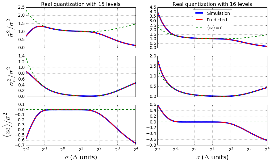
Results from simulations where we verify Equations  6 - 8 for the case of a real quantizer with $N=15$ levels (left column) and $N=16$ levels (right column) and a real Gaussian input are shown in Figure 1. From top to bottom row, the plots show the variance of the quantized output, $\hat{\sigma}^{2}$, the quantization error, $\sigma_{e}^{2}$, and the correlation between the input and quantization error $\langle ve\rangle$ as function of the unquantized standard deviation $\sigma$. All the values are normalized with respect to $\sigma^{2}$. For easier visualization of the results, especially in the low and high signal level regimes, the x-axis is in logarithmic scale (base 2, so the exponents can be interpeted as bits rms). For each plot, the red line corresponds to Equations 6 - 8 and the blue line (made thicker so it can be distinguished from the red line) corresponds to the results from simulations where, for each value of $\sigma$, $10^{6}$ samples of a Gaussian input are quantized with $N$ levels and then the statistics of the input, output and quantization error are calculated. As reference, we also include the green dashed line that shows to the expected behavior from the uncorrelated quantization noise model that assumes $\langle ve\rangle=0$ (see Thompson et al., 2017, for a detailed discussion). The black solid vertical line corresponds to the highest level of the quantizer (7 for $N=15$ and 8 for $N=16$) above which clipping occurs.

Figure 1: Behavior of a quantizer with $N=15$ levels (left column) and $N=16$ levels (right column) and a real-valued Gaussian input. From top to bottom row, the plots show the variance of the quantized output, $\hat{\sigma}^{2}$, the quantization error, $\sigma_{e}^{2}$, and the correlation between the input and quantization error, $\langle ve\rangle$, as function of the unquantized standard deviation $\sigma$. All the values are normalized with respect to $\sigma^{2}$. For each plot, the red line corresponds to Equations 6 - 8, the thick blue line shows the results from simulations, and the green dashed line corresponds to the uncorrelated quantization noise model that assumes $\langle ve\rangle=0$. Note that Equations 6 - 8 predict accurately the results from simulations. When the input $\sigma$ uses optimally the quantizer’s dynamic range the quantization error is very weakly correlated with the input. In this case the uncorrelated quantization noise model provides a very good approximation, introducing only a small bias error.

The first thing to note from Figure 1 is that Equations 6 - 8 predict accurately the results from simulations regarding $\hat{\sigma}^{2},~{}\sigma_{e}^{2}$, and $\langle ve\rangle$. Also that the uncorrelated quantization noise model provides an excellent approximation in the interval where $\langle ve\rangle\rightarrow 0$. For $N=15$, the value of $\sigma$ that minimizes the magnitude of the input-error correlation coefficient, $\rho_{ve}=\langle ve\rangle/(\sigma\sigma_{e})$, is $\sigma\approx 2^{0.14}\Delta$. At this point $|\rho_{ve}|\approx 5.5\times 10^{-10}$. For $N=16$ we have $\rho_{ve}=0$ for $\sigma\approx 2^{0.2}\Delta$. In both cases the minimum of $|\rho_{ve}|$ is broad so there is effectively a $\sigma$-interval, which we denote the interval of optimal quantization, for which the correlation between the input and quantization error is very weak and the uncorrelated quantization error model provides a very accurate approximation (the error in the calculated quantization parameters is negligible). The length of this interval depends on $N$ and on the tolerance required by each specific application. For example, if we require that $|\rho_{ve}|\lesssim 10^{-3}$ for $N=15$, then the interval of optimal quantization is, approximately, $[2^{-0.6},2^{0.9}]$. Within this interval the values of $\hat{\sigma}^{2}$ and $\sigma_{e}^{2}$ from the uncorrelated quantization error model agree with the values from Equations 6 - 8 at the $\sim 0.07\%$ level. The performance of the $N=16$ quantizer within this interval is similar.

Also note that, even in the high-$\sigma$ regime, where the quantization error resulting from clipping dominates and is correlated with the input, the uncorrelated quantization noise model also predicts with high accuracy the contribution of this overload error to $\sigma_{e}^{2}$ as the middle plot shows. However, it cannot track the quantized standard deviation (top plot) since in this regime $\langle ve\rangle<0$ which eventually makes $\hat{\sigma}^{2}/\sigma^{2}<1$ for large inputs. In the low-$\sigma$ regime, when $\sigma\lesssim 1/2$, the uncorrelated quantization noise model deviates from Equations 6 - 8 for two reasons: first, it is no longer true that the quantization error is uniformly distributed in the interval $[-\Delta/2,\Delta/2]$, and second, the behavior is now closer to that of a 3-bit ($N$ odd) or 2-bit ($N$ even) quantizer, so the quantization error is again correlated with the input. As $N$ increases, both the interval of optimal quantization and the accuracy of the uncorrelated quantization error model increase.

Finally, note that $\langle ve\rangle$ is negative (it approaches zero assymptotically) for $N=15$ while it becomes positive in the low signal level regime for $N=16$. Since the sum $S_{o}=\sum_{i=0}^{(N-3)/2}\mathcal{N}\left(\left.1/2+i\right|\sigma^{2}\right)$ in Equation 6 is positive and bounded above by 1/2 ($S_{o}<1/2$, a proof is provided in Appendix 8) then $\langle ve\rangle$ is always negative for $N$ odd. Furthermore, $\langle ve\rangle\in(-\sigma^{2},0)$ in this case. On the other hand, for $N$ even, the sum $S_{e}=\sum_{i=0}^{(N-4)/2}\mathcal{N}\left(\left.1+i\right|\sigma^{2}\right)$ is also positive and bounded above by 1/2, but the term $1/(\sqrt{2\pi\sigma^{2}})$ becomes arbitrarily large as $\sigma$ decreases. Thus, $\langle ve\rangle$ is always positive and unbounded for $N$ even in the low-$\sigma$ regime.

3 Complex-valued quantizer

In the CHIME correlator, the (real-valued) analog signal of each input is first digitized and then passed through the F-engine that implements a Polyphase Filter Bank (PFB) which splits the 400 MHz-wide input into 1024 frequency bins, each 390 kHz wide. The output of each frequency bin is a complex-valued signal and its real and imaginary parts are separately quantized with 15 levels before the data is re-arranged and sent to the X-engine for cross-multiplication and integration. In this section we extend the results of Section 2 to the case of an $N$-level complex-valued quantizer, where the real and imaginary parts of the input are separately quantized with $N$ levels. In this case we assume that the input $v=v_{r}+jv_{i}$ is a complex and circularly-symmetric Gaussian process such that $\langle v_{r}v_{i}\rangle=0$ and $\langle v_{r}^{2}\rangle=\langle v_{i}^{2}\rangle=\langle|v|^{2}\rangle/2$ where $\langle|v|^{2}\rangle=\sigma^{2}$ is the the unquantized standard deviation. As in Section 2 we are interested in the standard deviation of the quantization error, $e=e_{r}+je_{i}$, and its correlation with the input. In this case we have

$$\begin{split}\langle ve^{*}\rangle&=\langle(v_{r}+jv_{i})(e_{r}+je_{i})^{*}\rangle\\ &=\langle v_{r}e_{r}\rangle+\langle v_{i}e_{i}\rangle+j\left(-\langle v_{r}e_{i}\rangle+\langle v_{i}e_{r}\rangle\right).\end{split}$$ (9)

The circular symmetry of $v$ (its real and imaginary part are uncorrelated and have identical statistics) implies that $\langle v_{r}e_{r}\rangle=\langle v_{i}e_{i}\rangle$. As for $\langle v_{r}e_{i}\rangle$, note that, for the $m$-th imaginary quantization level we have

$$\begin{split}\langle v_{r}e_{i}\rangle_{m}&=\int_{y_{m-1}}^{y_{m}}\int_{-\infty}^{\infty}(k_{m}-v_{i})v_{r}f(v_{r},v_{i})dv_{r}dv_{i}\\ &=\int_{y_{m-1}}^{y_{m}}(k_{m}-v_{i})\mathcal{N}\left(v_{i}\left|\frac{\sigma^{2}}{2}\right.\right)dv_{i}\int_{-\infty}^{\infty}v_{r}\mathcal{N}\left(v_{r}\left|\frac{\sigma^{2}}{2}\right.\right)dv_{r}\\ &=0.\end{split}$$ (10)

Thus $\langle v_{r}e_{i}\rangle=0$ and, for the same reason, $\langle v_{i}e_{r}\rangle=0$. This means that $\langle ve^{*}\rangle$ is real and, from Equation 6

$$\langle ve^{*}\rangle=2\langle v_{r}e_{r}\rangle=\sigma^{2}\left[-1+\sum_{i=1}^{N-1}\mathcal{N}\left(\left.-\frac{N}{2}+i\right|\frac{\sigma^{2}}{2}\right)\right].$$ (11)

From the circular symmetry of $v$ it also follows that $\sigma_{e}^{2}=2\langle e_{r}^{2}\rangle$ and $\hat{\sigma}^{2}=2\langle\hat{v}_{r}^{2}\rangle$, so similar expressions for $\sigma_{e}^{2}/\sigma^{2}$ and $\hat{\sigma}^{2}/\sigma^{2}$ in the complex case are obtained from Equations 6 - 8 by changing $\sigma^{2}\rightarrow\sigma^{2}/2$.

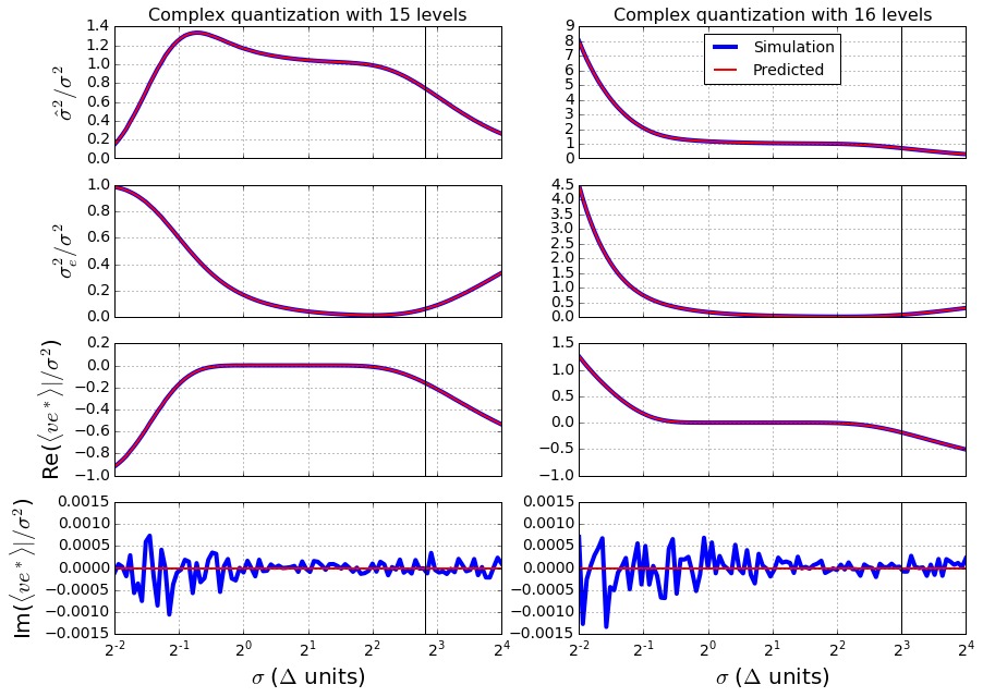
Results from simulations and comparison to our prediction for the complex-valued quantizer with $N=15$ levels (left column) and $N=16$ levels (right column) are shown in Figure 2. From top to bottom row, the plots show the normalized variance of the quantized output ($\hat{\sigma}^{2}/\sigma^{2}$), the quantization error ($\sigma_{e}^{2}/\sigma^{2}$), and the magnitude and phase (in degrees) of the normalized correlation between the input and quantization error ($\langle ve^{*}\rangle/\sigma^{2}$). For each plot, the red line is our prediction and the blue line corresponds to the results from simulations where, for each value of $\sigma$, $10^{6}$ samples of a complex and circularly-symmetric Gaussian input are quantized with $N$ levels (real and imaginary parts quantized separately) and then the statistics of the input, output and quantization error are calculated.

Figure 2: Behavior of a complex-valued quantizer with $N=15$ levels (left column) and $N=16$ levels (right column) and a circularly-symmetric Gaussian input. From top to bottom row, the plots show the normalized variance of the quantized output ($\hat{\sigma}^{2}/\sigma^{2}$), the quantization error ($\sigma_{e}^{2}/\sigma^{2}$), and the magnitude and phase (in degrees) of the normalized correlation between the input and quantization error ($\langle ve^{*}\rangle/\sigma^{2}$). For each plot, the red line is our prediction and the blue line is the result from simulations. There is again excellent agreement between these. Note that $\langle ve^{*}\rangle$ is always real (in the simulation the imaginary part is consistent with zero at the $\sim$ 0.15% level), and it is negative ($180^{\circ}$ phase) for $N$ odd, while it becomes positive ($0^{\circ}$ phase) in the low $\sigma$ regime for $N$ even.

There is again excellent agreement between the simulations and the predictions. The correlation between the input and quantization error, $\langle ve^{*}\rangle$, is always real (in the simulation the imaginary part is consistent with zero at the $\sim$ 0.15% level). Furthermore, it is always negative ($180^{\circ}$ phase) for $N$ odd, while it becomes positive ($0^{\circ}$ phase) in the low $\sigma$ regime for $N$ even. In this case the optimal quantization interval corresponding to $|\rho_{ve}|\lesssim 10^{-3}$ is approximately $[2^{-0.1},2^{1.4}]$ (the interval shifts by $\sqrt{2}$ with respect to the real-valued case).

4 Real-valued correlator

The correlation between two real-valued quantized inputs $\hat{v}_{1}$ and $\hat{v}_{2}$, is

$$\hat{r}_{12}=\langle\hat{v}_{1}\hat{v}_{2}\rangle.$$ (12)

The output of a real-valued digital correlator after integrating $N_{s}$ samples is

$$\hat{r}_{12,N_{s}}=\frac{1}{N_{s}}\sum_{n=1}^{N_{s}}\hat{v}_{1}[n]\hat{v}_{2}[n].$$ (13)

Since the quantized sample vector $(\hat{v}_{1}[n],\hat{v}_{2}[n])$ comes from the IID joint Gaussian process $(v_{1},v_{2})$, then $\langle\hat{r}_{12,N_{s}}\rangle=\hat{r}_{12}$ so the measured correlation $\hat{r}_{12,N_{s}}$ is an unbiased estimator of $\hat{r}_{12}$. Henceforth we will refer to $\hat{r}_{12}$ as the output of the digital correlator.

Note that we already investigated the behavior of $\hat{r}_{11}=\hat{\sigma}_{1}^{2}$ and $\hat{r}_{22}=\hat{\sigma}_{2}^{2}$ in Section 2 (the result in this case is the same because the marginal PDFs of $v_{1}$ and $v_{2}$ are independent of the correlation between inputs). Now we are interested in $\hat{r}_{12}$ and its relation to $r_{12}=\langle v_{1}v_{2}\rangle$ which is the correlation between the unquantized inputs $v_{1}$ and $v_{2}$ and what we ultimately want to measure. We can write $\hat{r}_{12}$ as

$$\begin{split}\hat{r}_{12}&=\langle(v_{1}+e_{1})(v_{2}+e_{2})\rangle\\ &=r_{12}+\langle v_{1}e_{2}\rangle+\langle e_{1}v_{2}\rangle+\langle e_{1}e_{2}\rangle\end{split}$$ (14)

where

$$\begin{split}\langle v_{1}e_{2}\rangle&=\sum_{i=1}^{N}\int_{y_{i-1}}^{y_{i}}\int_{-\infty}^{\infty}(k_{i}-v_{2})v_{1}f(v_{1},v_{2})dv_{1}dv_{2}\\ \end{split}$$ (15)

and

$$\begin{split}\langle e_{1}e_{2}\rangle&=\sum_{j=1}^{N}\sum_{i=1}^{N}\int_{y_{j-1}}^{y_{j}}\int_{y_{i-1}}^{y_{i}}(k_{i}-v_{1})(k_{j}-v_{2})f(v_{1},v_{2})dv_{1}dv_{2}.\end{split}$$ (16)

$\langle e_{1}v_{2}\rangle$ is defined as in Equation 15. If the samples from $v_{1}$ and $v_{2}$ come from a zero-mean joint Gaussian PDF

$$\mathcal{N}\left(v_{1},v_{2}\left|\sigma_{1}^{2},\sigma_{2}^{2},\rho\right.\right)=\frac{1}{2\pi\sigma_{1}\sigma_{2}\sqrt{1-\rho^{2}}}e^{-\frac{1}{2(1-\rho^{2})}\left[\frac{v_{1}^{2}}{\sigma_{1}^{2}}+\frac{v_{2}^{2}}{\sigma_{2}^{2}}-\frac{2\rho v_{1}v_{2}}{\sigma_{1}\sigma_{2}}\right]}$$ (17)

where $\rho=\langle v_{1}v_{2}\rangle/(\sigma_{1}\sigma_{2})$, then Equation 15 can be simplified

$$\begin{split}\langle v_{1}e_{2}\rangle&=\sum_{i=1}^{N}\int_{y_{i-1}}^{y_{i}}\int_{-\infty}^{\infty}(k_{i}-v_{2})v_{1}\mathcal{N}\left(v_{1},v_{2}\left|\sigma_{1}^{2},\sigma_{2}^{2},\rho\right.\right)dv_{1}dv_{2}\\ &=\rho\frac{\sigma_{1}}{\sigma_{2}}\sum_{i=1}^{N}\int_{y_{i-1}}^{y_{i}}(k_{i}-v_{2})v_{2}\mathcal{N}\left(v_{2}|\sigma_{2}^{2}\right)dv_{2}\\ &=\rho\frac{\sigma_{1}}{\sigma_{2}}\langle v_{2}e_{2}\rangle\\ &=r_{12}\frac{\langle v_{2}e_{2}\rangle}{\sigma_{2}^{2}}.\end{split}$$ (18)

Similarly $\langle e_{1}v_{2}\rangle=r_{12}\langle v_{1}e_{1}\rangle/\sigma_{1}^{2}$. Note that with this result we can find both $\langle v_{1}e_{2}\rangle$ and $\langle e_{1}v_{2}\rangle$, which are correlations between mixed input-error terms, using Equation 6 for the correlation between an input and its respective quantization error.

As for $\langle e_{1}e_{2}\rangle$ in Equation 16, it can be simplified in the case when $\rho$ is small, since in this regime we have

$$\left.\mathcal{N}\left(v_{1},v_{2}\left|\sigma_{1}^{2},\sigma_{2}^{2},\rho\right.\right)\right|_{\rho\ll 1}\approx\mathcal{N}(v_{1}|\sigma_{1}^{2})\mathcal{N}(v_{2}|\sigma_{2}^{2})\left(1+\frac{\rho v_{1}v_{2}}{\sigma_{1}\sigma_{2}}\right)$$ (19)

so

$$\begin{split}\left.\langle e_{1}e_{2}\rangle\right|_{\rho\ll 1}\approx&\sum_{i=1}^{N}\int_{y_{i-1}}^{y_{i}}(k_{i}-v_{1})\mathcal{N}(v_{1}|\sigma_{1}^{2})dv_{1}\sum_{j=1}^{N}\int_{y_{j-1}}^{y_{j}}(k_{j}-v_{2})\mathcal{N}(v_{2}|\sigma_{2}^{2})dv_{2}\\ &+\frac{\rho}{\sigma_{1}\sigma_{2}}\sum_{i=1}^{N}\int_{y_{i-1}}^{y_{i}}(k_{i}-v_{1})v_{1}\mathcal{N}(v_{1}|\sigma_{1}^{2})dv_{1}\sum_{j=1}^{N}\int_{y_{j-1}}^{y_{j}}(k_{j}-v_{2})v_{2}\mathcal{N}(v_{2}|\sigma_{2}^{2})dv_{2}\\ =&\langle e_{1}\rangle\langle e_{2}\rangle+\frac{\rho}{\sigma_{1}\sigma_{2}}\langle v_{1}e_{1}\rangle\langle v_{2}e_{2}\rangle\\ =&r_{12}\frac{\langle v_{1}e_{1}\rangle}{\sigma_{1}^{2}}\frac{\langle v_{2}e_{2}\rangle}{\sigma_{2}^{2}}.\end{split}$$ (20)

Equation 20 will be useful when we analyze the phase behavior of the complex-valued correlator.

From Equations 14 and 18 we can write

$$\begin{split}\hat{r}_{12}&=r_{12}\left(1+\frac{\langle v_{1}e_{1}\rangle}{\sigma_{1}^{2}}+\frac{\langle v_{2}e_{2}\rangle}{\sigma_{2}^{2}}\right)+\langle e_{1}e_{2}\rangle\end{split}$$ (21)

and, using Equation 20

$$\begin{split}\left.\hat{r}_{12}\right|_{\rho\ll 1}\approx&~{}r_{12}\left(1+\frac{\langle v_{1}e_{1}\rangle}{\sigma_{1}^{2}}+\frac{\langle v_{2}e_{2}\rangle}{\sigma_{2}^{2}}+\frac{\langle v_{1}e_{1}\rangle}{\sigma_{1}^{2}}\frac{\langle v_{2}e_{2}\rangle}{\sigma_{2}^{2}}\right)=r_{12}\left(1+\frac{\langle v_{1}e_{1}\rangle}{\sigma_{1}^{2}}\right)\left(1+\frac{\langle v_{2}e_{2}\rangle}{\sigma_{2}^{2}}\right).\end{split}$$ (22)

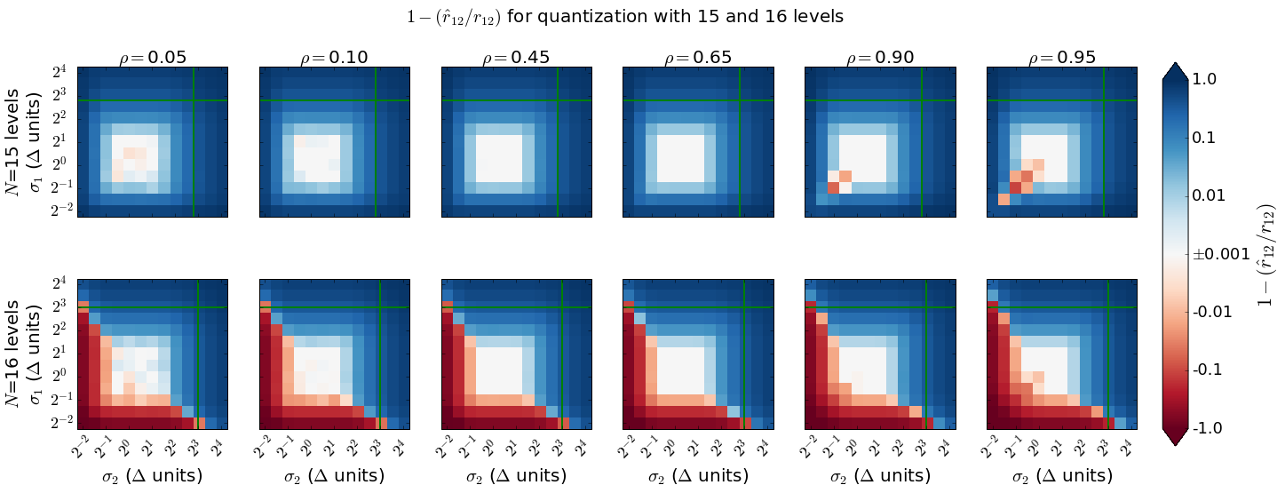
The behavior from simulations of the normalized and quantized input correlation $r=\hat{r}_{12}/r_{12}$ and the contribution of the correlation between the quantization errors of the two inputs, $\langle e_{1}e_{2}\rangle$ (also normalized by $r_{12}$) are shown in Figures 3 and 4 respectively. For each value of $\sigma_{1},~{}\sigma_{2}$ and $\rho$, $10^{7}$ sample vectors $(v_{1}[n],v_{2}[n])$ from the joint Gaussian distribution in Equation 17 are quantized with $N$ levels and then both $\hat{r}_{12}$ and $\langle e_{1}e_{2}\rangle$ are calculated and normalized by the (measured) unquantized input correlation $r_{12}$. The axes for each plot are the unquantized input signal levels and the green solid lines correspond to the highest level of the quantizer (7 for $N=15$ and 8 for $N=16$) above which clipping occurs.

Figure 3: Results from simulations of $r=\hat{r}_{12}/r_{12}$ as function of $\sigma_{1}$ and $\sigma_{2}$ for different values of $\rho$ for a real correlator with $N=15$ levels (top row) and $N=16$ levels (bottom row). The axes for each plot are the unquantized input signal levels and the green solid lines correspond to the highest level of the quantizer above which clipping occurs. The bias in $\hat{r}_{12}$ for moderate values of $\rho$ ($|\rho|\lesssim 0.85$) is below $\sim 0.1\%$ approximately within the inner white square enclosed by the region $\sigma_{1}\times\sigma_{2}\approx[2^{-0.6},2^{0.9}]\times[2^{-0.6},2^{0.9}]$. For $|\rho|\gtrsim 0.85$ the bias can increase up to $\sim 4\%$.

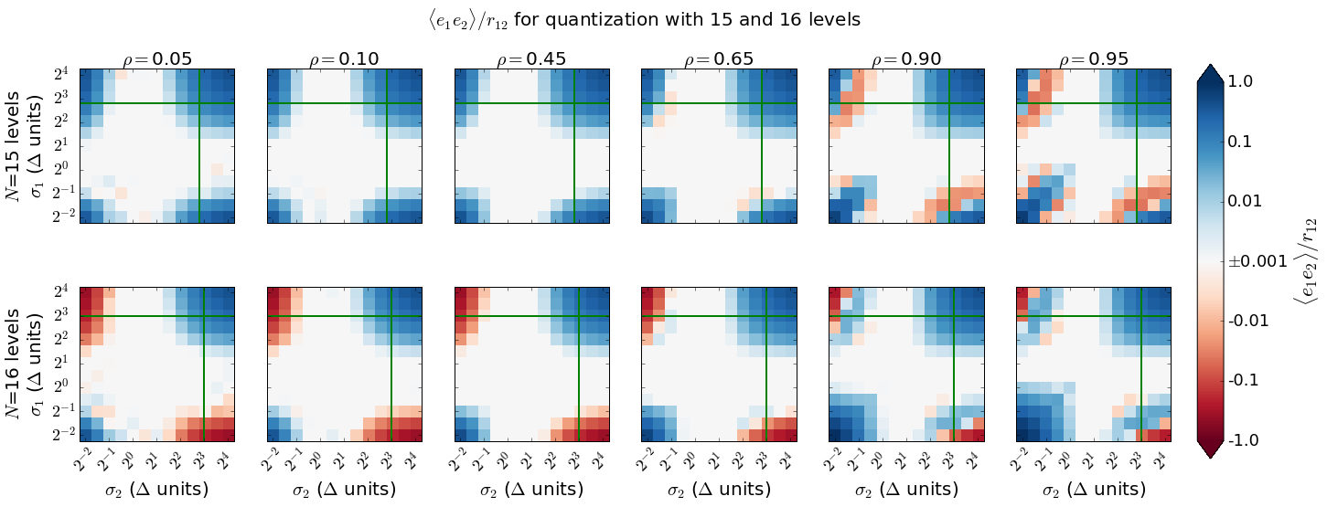
Figure 4: Correlation between the quantization errors of the two inputs, $\langle e_{1}e_{2}\rangle$ (normalized by $r_{12}$), as function of $\sigma_{1},~{}\sigma_{2}$ and $\rho$, from simulations. Note that $e_{1}$ and $e_{2}$ are very weakly correlated as long as at least one of the two inputs is optimally quantized.

With $10^{7}$ samples, the values in each pixel of Figure 3 agree with the values from Equation 21 with unbiased error fluctuations below $\sim$ 1%. The worst case corresponds to low values of $\sigma$ and $\rho$ where $r_{12}$ is very small. These results confirm that Equation 21 accurately reproduces the relation between $\hat{r}_{12}$ and $r_{12}$ for the real-valued correlator.

For moderate values of $\rho$ ($|\rho|\lesssim 0.85$) the bias in $\hat{r}_{12}$ (Figure 3) is below $\sim 0.1\%$ (values from Equation 21) approximately within the inner white square enclosed by the region $\sigma_{1}\times\sigma_{2}\approx[2^{-0.6},2^{0.9}]\times[2^{-0.6},2^{0.9}]$, corresponding to the region where both inputs are optimally quantized (see Section 2). For $|\rho|\gtrsim 0.85$ the bias within this region can increase up to $\sim 4\%$.

The most important feature from Figure 4 is that $e_{1}$ and $e_{2}$ are weakly correlated as long as at least one of the two inputs is approximately uncorrelated with its respective quantization error (either $\langle v_{1}e_{1}\rangle$ or $\langle v_{2}e_{2}\rangle$ is negligible). Another way to say this is that $e_{1}$ and $e_{2}$ are weakly correlated as long as at least one of the two inputs is optimally quantized, i.e., when the model of additive uncorrelated quantization noise is (approximately) valid. Note that this is what one would intuitively assume using the nominal model of additive uncorrelated quantization error. We will use this result when we analyze the phase of the measured correlation in a complex correlator.

5 Complex-valued correlator

Now we extend the results from Section 4 to the case when the correlator inputs are complex-valued, such as for the complex channelization stage of the CHIME correlator, where the digitized inputs are channelized using a PFB that splits the 400 MHz-wide input into 1024 narrow frequency bins. The complex-valued output of each frequency bin is quantized with $N=15$ levels for both the real and imaginary parts. Finally, the quantized signals are sent to the correlator that measures complex-valued correlation between quantized inputs, $\hat{r}_{12}=\langle\hat{v}_{1}\hat{v}_{2}^{*}\rangle$. We are ultimately interested in $r_{12}=\langle v_{1}v_{2}^{*}\rangle$ so we need to find a relation between these.

As in Section 3, we assume that $\bm{v}=(v_{1},v_{2})$ is a complex and circularly-symmetric Gaussian process. Then

$$\begin{split}\hat{r}_{12}&=\langle(\hat{v}_{1r}+j\hat{v}_{1i})(\hat{v}_{2r}-j\hat{v}_{2i})\rangle\\ &=\langle\hat{v}_{1r}\hat{v}_{2r}\rangle+\langle\hat{v}_{1i}\hat{v}_{2i}\rangle+j\left(-\langle\hat{v}_{1r}\hat{v}_{2i}\rangle+\langle\hat{v}_{1i}\hat{v}_{2r}\rangle\right)\end{split}$$ (23)

The circular symmetry of $\bm{v}$ implies that $\langle\hat{v}_{1r}\hat{v}_{2r}\rangle=\langle\hat{v}_{1i}\hat{v}_{2i}\rangle$ and $-\langle\hat{v}_{1r}\hat{v}_{2i}\rangle=\langle\hat{v}_{1i}\hat{v}_{2r}\rangle$ so

$$\begin{split}\hat{r}_{12}&=2\left[\langle\hat{v}_{1r}\hat{v}_{2r}\rangle+j\langle\hat{v}_{1i}\hat{v}_{2r}\rangle\right]\\ &=2(\hat{r}_{1r,2r}+j\hat{r}_{1i,2r})\end{split}$$ (24)

Now, for $\hat{r}_{1r,2r}=\langle\hat{v}_{1r}\hat{v}_{2r}\rangle$ and $\hat{r}_{1i,2r}=\langle\hat{v}_{1i}\hat{v}_{2r}\rangle$ which are real, we can use Equation 21 so

$$\begin{split}\hat{r}_{12}&=2\left\{\left[r_{1r,2r}\left(1+\frac{\langle v_{1r}e_{1r}\rangle}{\sigma_{1r}^{2}}+\frac{\langle v_{2r}e_{2r}\rangle}{\sigma_{2r}^{2}}\right)+\langle e_{1r}e_{2r}\rangle\right]+j\left[r_{1i,2r}\left(1+\frac{\langle v_{1i}e_{1i}\rangle}{\sigma_{1i}^{2}}+\frac{\langle v_{2r}e_{2r}\rangle}{\sigma_{2r}^{2}}\right)+\langle e_{1i}e_{2r}\rangle\right]\right\}\\ &=2\left(r_{1r,2r}+jr_{1i,2r}\right)\left(1+\frac{\langle v_{1r}e_{1r}\rangle}{\sigma_{1r}^{2}}+\frac{\langle v_{2r}e_{2r}\rangle}{\sigma_{2r}^{2}}\right)+2\left(\langle e_{1r}e_{2r}\rangle+j\langle e_{1i}e_{2r}\rangle\right)\\ &=r_{12}\left(1+\frac{\langle v_{1r}e_{1r}\rangle}{\sigma_{1r}^{2}}+\frac{\langle v_{2r}e_{2r}\rangle}{\sigma_{2r}^{2}}\right)+2\left(\langle e_{1r}e_{2r}\rangle+j\langle e_{1i}e_{2r}\rangle\right)\end{split}$$ (25)

where in the second step we used the fact that $\langle v_{1r}e_{1r}\rangle/\sigma_{1r}^{2}=\langle v_{1i}e_{1i}\rangle/\sigma_{1i}^{2}$ and in the third step we used $r_{12}=2\left(r_{1r,2r}+jr_{1i,2r}\right)$. All these follow from circular symmetry. Note that all the terms in Equation 25 can be obtained from Equations 6 and 16 using $\sigma_{1r}^{2}=\sigma_{1i}^{2}=\sigma_{1}^{2}/2$ and $\sigma_{2r}^{2}=\sigma_{2i}^{2}=\sigma_{2}^{2}/2$.

We can use Equation 25 to draw some important conclusions regarding how quantization affects the magnitude and phase of $r_{12}$. We can write

$$\hat{r}_{12}=\alpha r_{12}+\beta,\hskip 36.135pt\alpha=\left(1+\frac{\langle v_{1r}e_{1r}\rangle}{\sigma_{1r}^{2}}+\frac{\langle v_{2r}e_{2r}\rangle}{\sigma_{2r}^{2}}\right),\hskip 36.135pt\beta=2\left(\langle e_{1r}e_{2r}\rangle+j\langle e_{1i}e_{2r}\rangle\right)$$ (26)

Note that $\alpha$ is real, independent of $\rho$, and only contributes to the biasing of the magnitude of $\hat{r}_{12}$. On the other hand, $\beta$ is complex in general and affects both the magnitude and phase of $\hat{r}_{12}$.

Quantization will bias the magnitude of $\hat{r}_{12}$ except when $\alpha=1$ and $\beta=0$. This occurs approximately when both inputs are optimally quantized since in this case $\langle v_{1r}e_{1r}\rangle\rightarrow 0$, $\langle v_{2r}e_{2r}\rangle\rightarrow 0$ (so $\alpha\rightarrow 1$, see Section 2 and Figure 1), and also $\langle e_{1r}e_{2r}\rangle\rightarrow 0$, $\langle e_{1i}e_{2r}\rangle\rightarrow 0$ (so $\beta\rightarrow 0$, see Section 4 and Figure 4).

Quantization will bias the phase of $\hat{r}_{12}$ except in two cases: the first case is when $\beta=0$, which occurs approximately when at least one of the inputs is optimally quantized (see Section 4 and Figure 4). Note that this is a less stringent requirement than that for unbiased magnitude, which requires both inputs to be optimally quantized.

The second case for negligible bias in the phase of $\hat{r}_{12}$ occurs when $\rho\ll 1$ since using Equation 20 in Equation 25 we have

$$\begin{split}\left.\hat{r}_{12}\right|_{\rho\ll 1}&\approx 2r_{1r,2r}\left(1+\frac{\langle v_{1r}e_{1r}\rangle}{\sigma_{1r}^{2}}\right)\left(1+\frac{\langle v_{2r}e_{2r}\rangle}{\sigma_{2r}^{2}}\right)+2jr_{1i,2r}\left(1+\frac{\langle v_{1i}e_{1i}\rangle}{\sigma_{1i}^{2}}\right)\left(1+\frac{\langle v_{2r}e_{2r}\rangle}{\sigma_{2r}^{2}}\right)\\ &=r_{12}\left(1+\frac{\langle v_{1r}e_{1r}\rangle}{\sigma_{1r}^{2}}\right)\left(1+\frac{\langle v_{2r}e_{2r}\rangle}{\sigma_{2r}^{2}}\right).\end{split}$$ (27)

Since the factors that multiply $r_{12}$ are real then $\angle\left(\hat{r}_{12}\right)=\angle\left(r_{12}\right)$.

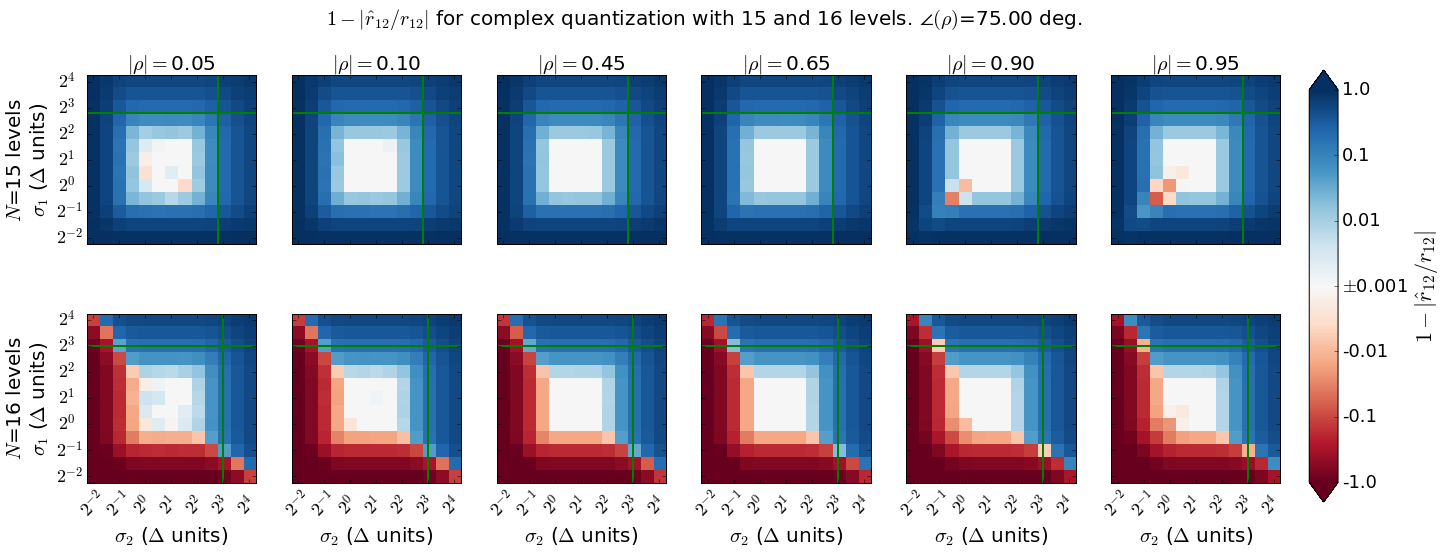
Figures 5 and 6 show results from simulations of $\hat{r}_{12}/r_{12}$ (magnitude and phase respectively. The phase is in degrees). The method is the same as in Section 2, but this time the $10^{7}$ sample vectors $(v_{1}[n],v_{2}[n])$ are drawn from a circularly symmetric Gaussian distribution. We only vary the magnitude of $\rho$, keeping its phase fixed at 75 degrees.

Note that Equations 25-27 predict accurately the behavior of the magnitude and phase of $\hat{r}_{12}$. For moderate values of $\rho$ ($|\rho|\lesssim 0.85$) the bias in the magnitude (Figure 5) is below $\sim 0.1\%$ roughly within the inner square enclosed by the region $\sigma_{1}\times\sigma_{2}\approx[2^{-0.1},2^{1.4}]\times[2^{-0.1},2^{1.4}]$, corresponding to region where both inputs are optimally quantized (see Section 3). For $|\rho|\gtrsim 0.85$ the bias within this region can increase up to $\sim 4\%$.

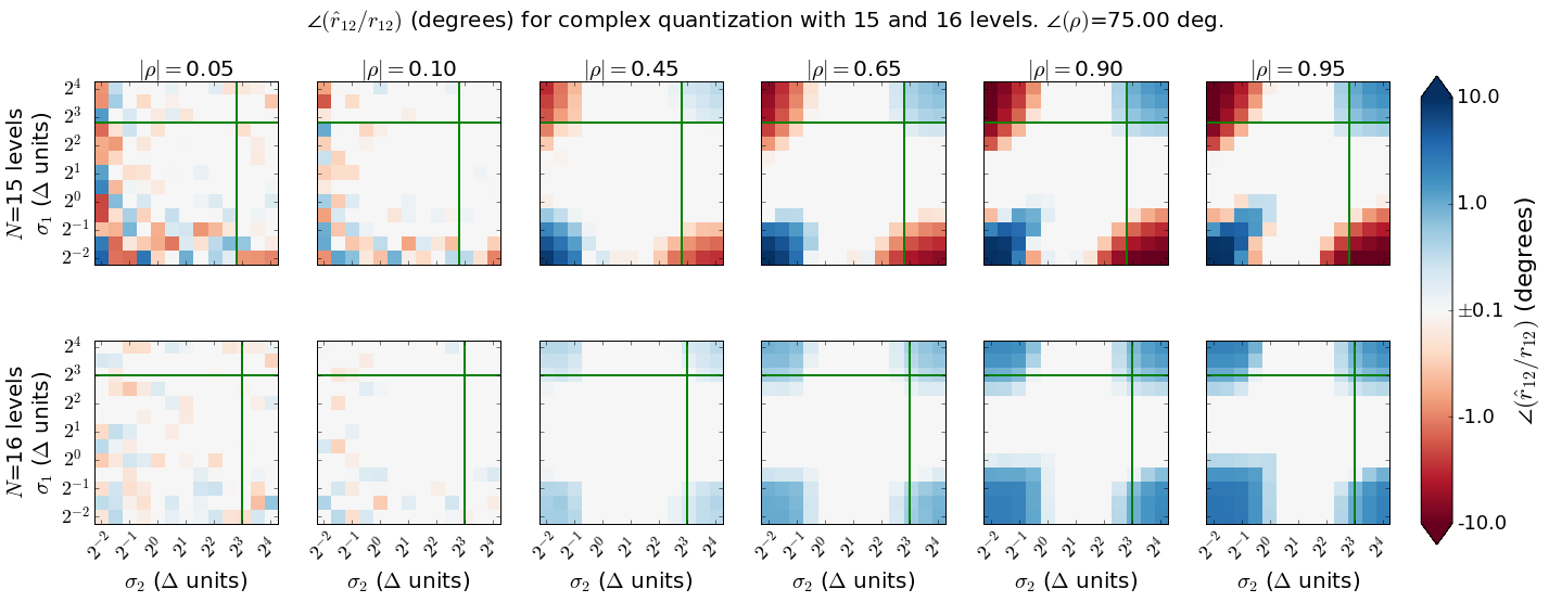
As for the phase (Figure 6), the bias is below $\sim 0.1^{\circ}$ within the cross-shaped region where either $\sigma_{1}$ or $\sigma_{2}$ are optimally quantized. When $|\rho|\gtrsim 0.85$ the bias within this region can rise up to $\sim 1^{\circ}$. When $\rho\lesssim 0.1$ (first two columns of Figure 6) the phase bias is below $\sim 0.1^{\circ}$ (values from Equation 25) for all values of $\sigma_{1}$ and $\sigma_{2}$ as predicted by Equation 27, although there are still random fluctuations in the simulation at the $\sim$ sub-degree level for very low values of $\sigma$ (bottom and left edges of the plots) for reasons explained in Section 4.

Figure 5: $|\hat{r}_{12}/r_{12}|$ from simulations as function of $\sigma_{1}$ and $\sigma_{2}$ for different values of $|\rho|$. For moderate values of $\rho$ the bias in the magnitude of $|\hat{r}_{12}|$ is below $\sim 0.1\%$ within the inner square enclosed by the region $\sigma_{1}\times\sigma_{2}\approx[2^{-0.1},2^{1.4}]\times[2^{-0.1},2^{1.4}]$, corresponding to region where both inputs are optimally quantized. For $|\rho|\gtrsim 0.85$ this bias can increase up to $\sim 4\%$.

Figure 6: $\angle(\hat{r}_{12}/r_{12})$ (in degrees) from simulations as function of $\sigma_{1}$ and $\sigma_{2}$ for different values of $|\rho|$. The bias in the phase of $\hat{r}_{12}$ is negligible when at least one of the inputs is optimally quantized. This is a less stringent requirement than that for the magnitude, which requires both inputs to be optimally quantized. The bias is below $\sim 0.1^{\circ}$ within the cross-shaped region where either $\sigma_{1}$ or $\sigma_{2}$ are in the approximate interval $[2^{-0.1},2^{1.4}]$. When $|\rho|$ is high (last two columns) the bias within this region can rise up to $\sim 1^{\circ}$. When $|\rho|$ is small (first two columns) the phase bias is below $\sim 0.1^{\circ}$ for all values of $\sigma_{1}$ and $\sigma_{2}$, although there are still random fluctuations in the simulation at the $\sim$ sub-degree level for very low values of $\sigma$ (see text).

6 Implications for radio interferometry

The results above have important implications for radio interferometry. Quantization will have a significant biasing effect on the visibility magnitude unless both inputs are optimally quantized, which can be a stringent requirement (both signal levels need to be in the region where the uncorrelated quantization model is valid). However, we have found that the bias in the visibility phase is negligible even in conditions as extreme as when one of the inputs is suffering from severe clipping, or even when both inputs are severely clipped in the case of weak sources ($|\rho|\ll 1$). The same conditions apply when one or both input levels are very low (note that any of these extreme conditions will affect the signal-to-noise ratio of the measured visibility even if the phase is unbiased, but that analysis is beyond the scope of this paper). An accurate determination of the visibility phase is critical for beamforming, fringe stopping, and image reconstruction techniques.

For the particular case of CHIME, in which the sky signals are weak and the correlator inputs are dominated by the noise of the analog receiving system, the correlation coefficient is typically low ($|\rho|\lesssim 0.1$) even for the brightest radio point sources such as CasA, CygA, and TauA, but excluding the sun. This means that, except for the time when the sun is in the primary beam of the CHIME telescope ($\sim 14$ minutes per day), all the visibility phases will have negligible bias due to quantization.

The quantization bias also has an effect on the beamformed sensitivity of a radio interferometric array. To illustrate this, consider a one-dimensional array consisting of uniformly spaced feeds located at positions $0,1,\ldots,N_{f}-1$, in units of the normalized feed spacing $b_{\lambda}=b/\lambda$, where $\lambda$ is the observed wavelength. This example corresponds to one of the cylinders of the CHIME telescope, where the feeds are uniformly spaced along the axis of the cylinder. The cylinder axis (and thus the linear array) is oriented North-South (N-S), so the resolution in the N-S direction is provided by the correlations between feeds. We will assume that all the feeds have identical beams that are N-S isotropic and receivers with system noise $\sigma_{sys}^{2}$, although the generalization is straightforward.

For a point source on the meridian with noise temperature $\sigma^{2}$ such that the signal-to-system-noise ratio is $SNR=\sigma^{2}/\sigma_{sys}^{2}$, the unquantized autocorrelations for each feed are identical and equal to

$$r_{ii}=\sigma_{sys}^{2}(1+SNR),\hskip 36.135pti=0,1,\ldots,N_{f}-1$$ (28)

while the unquantized visibility and correlation coefficient between feeds $i$ and $j$ are

$$r_{ij}=SNR\cdot\sigma_{sys}^{2}e^{-j2\pi(i-j)b_{\lambda}\sin\theta},\hskip 36.135pt\rho_{ij}=\frac{e^{-j2\pi(i-j)b_{\lambda}\sin\theta}}{1+\frac{1}{SNR}}$$ (29)

where $\theta$ is the source zenith angle and we have assumed uncorrelated system noise between feeds.

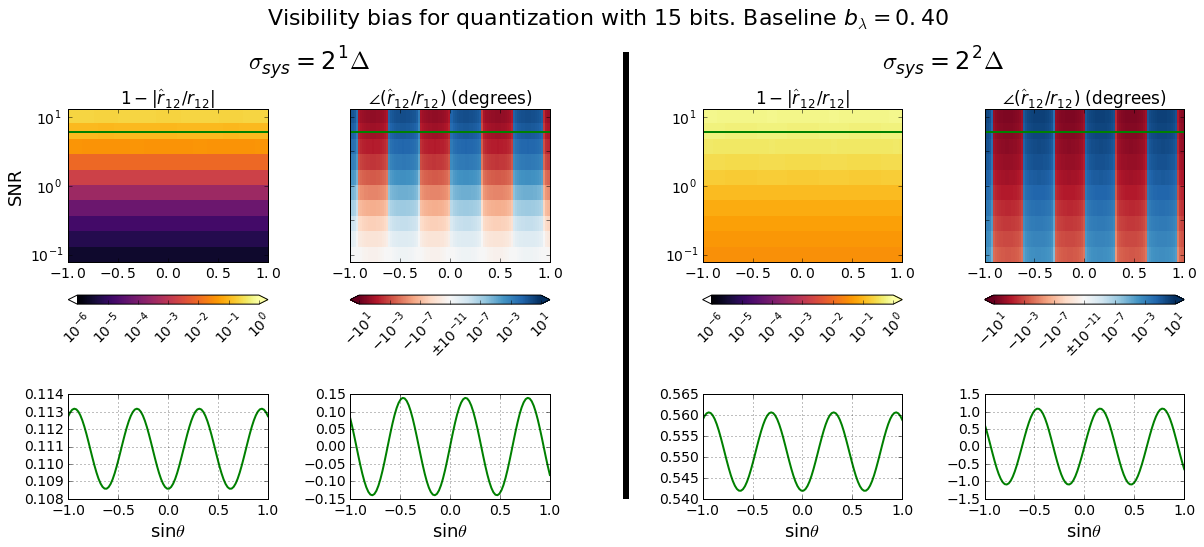
The bias due to quantization of the measured visibility as function of $SNR$ and $\theta$ for $i=j+1$ (consecutive feeds) is shown in Figure 7. We use $b_{\lambda}=0.4$ which corresponds to the CHIME normalized feed spacing at 400 MHz. These results are obtained directly from Equation 25.

Figure 7: Bias due to quantization of the measured visibility as function of the source position $\theta$ and the signal-to-system-noise ratio is $SNR$. The visibility baseline is $b_{\lambda}=0.4$ which corresponds to the CHIME normalized feed spacing at 400 MHz. When $\sigma_{sys}=2^{1}\Delta$ (left panels), well within the optimal quantization interval, the quantization bias for weak sources ($SNR\lesssim 0.1$) is negligible. This is the regime for CHIME $\sim 99\%$ of the time. When $\sigma_{sys}=2^{1}\Delta$ (right panels), which is the optimal input level according to the uncorrelated quantization noise model, the amount of bias increases significantly.

To illustrate the difference between Equation 25 and the uncorrelated quantization noise model, and the importance of optimizing the input signal level of the quantizer, Figure 7 shows the bias for two different values of $\sigma_{sys}$: $2^{1}\Delta$ (left panels) and $2^{2}\Delta$ (right panels). For a system-noise dominated telescope like CHIME, the correlator inputs are calibrated so $\sigma_{sys}$ corresponds to the optimal input level of the quantizer in order to minimize the effects of quantization. For $N=15$, the optimal input level according to the uncorrelated quantization noise model is $\sigma_{sys}\approx 2^{2}\Delta$, corresponding to the point where $\sigma_{e}$ is minimum (see second row of Figure 2). On the other hand, Equation 25 suggests that a better choice for $\sigma_{sys}$ should be more centered around the optimal quantization interval $[2^{-0.1}\Delta,2^{1.4}\Delta]$. The CHIME digital calibration module uses $\sigma_{sys}\approx 2^{1}\Delta$, which is well within this interval while still keeping $\sigma_{e}$ relatively low (see second and third rows of Figure 2, if $\sigma_{sys}$ is too close to the lower end of the interval then the contribution of $\sigma_{e}$ is significant).

Note that the $SNR$ sets the overall amount of bias due to quantization since this parameter defines both $r_{ii}$ and $|\rho_{ij}|$ (Equations 28 and 29). For $\sigma_{sys}=2^{1}\Delta$ and $|\rho_{ij}|\lesssim 0.1$ (so $SNR\lesssim 0.1$) the magnitude bias is $\lesssim 10^{-6}$ and the phase bias is $\lesssim 10^{-11}$ degrees, too small to have any significant impact that requires the generalized Van Vleck correction from Benkevitch et al. (2016). As mentioned before, this is the regime for CHIME $\sim 99\%$ of the time. However, when the sun is in the main beam ($\sim 1\%$ of the time), the $SNR$ can be as high as $\sim 6$ (green line in Figure 7), corresponding to a magnitude bias of $\sim 11\%$ and a phase bias of up to $\sim 0.15^{\circ}$. Although the CHIME cosmology data pipeline masks out the sun time, this data is still very useful for beam mapping purposes. The quantization bias is significant enough in this case to justify the implementation of the generalized Van Vleck correction.

When $\sigma_{sys}=2^{2}\Delta$ (right side of Figure 7) the amount of bias increases significantly even in the weak-source regime. For $SNR\sim 0.1$ the magnitude bias is $\sim 3\%$ and the phase bias is $\sim 3\times 10^{-3}$ degrees, while for $SNR\sim 6$ the magnitude bias is $\sim 56\%$ and the phase bias is $\sim 1^{\circ}$, demonstrating that for this particular application the uncorrelated quantization noise model must be used carefully since it can introduce important effects in the measured visibilities.

The quantization bias also depends on the position of the source and the baseline. These parameters determine $\angle(\rho_{ij})$ which affects the measured visibility $\hat{r}_{ij}$ through the second term of Equation 25. As Figure 7 shows, the position dependence manifests as fringes as a function of $l=\sin\theta$, where the baseline determines the quantization fringe rate.

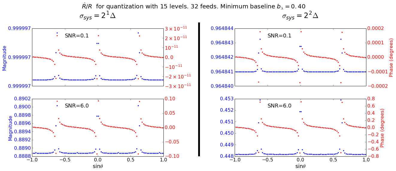
We can use the $N_{f}(N_{f}-1)/2$ visibilities (excluding the autocorrelations) to beamform in the direction of the source. Since for $k=i-j$ fixed there are $(N_{f}-k)$ identical baselines, then we can write the quantized beamformed output as

$$\begin{split}\hat{R}&=\sum_{i>j}^{N_{f}-1}\hat{r}_{ij}e^{j2\pi(i-j)b_{\lambda}\sin\theta}=\sum_{k=1}^{N_{f}-1}(N_{f}-k)\hat{r}_{k}e^{j2\pi kb_{\lambda}\sin\theta}\end{split}$$ (30)

while the unquantized beamformed output is

$$\begin{split}R&=\sum_{k=1}^{N_{f}-1}(N_{f}-k)r_{k}e^{j2\pi kb_{\lambda}\sin\theta}=\frac{N_{f}(N_{f}-1)}{2}SNR\sigma_{sys}^{2}.\end{split}$$ (31)

We can define a complex quantization parameter

$$\eta_{q}=\frac{\hat{R}}{R}$$ (32)

as a measure of the beamforming efficiency due to quantization. Figure 8 shows the magnitude and phase of $\eta_{q}$ as function of the source position $\theta$ for $SNR=0.1$ (approximate upper limit of weak-source regime) and $SNR=6$ (typical strong source like the sun). We used $N_{f}=32$ and kept $b_{\lambda}$ fixed at 0.4.

Figure 8: Complex quantization parameter $\eta_{q}=\hat{R}/R$ as function of the source position $\theta$ for $SNR=0.1$ (top row, this $SNR$ is the approximate upper limit of weak-source regime) and $SNR=6$ (bottom row, this is the typical $SNR$ of a strong source like the sun). For each plot, the blue labels and dots correspond to the magnitude of $\eta_{q}$ and the red labels and dots correspond to its phase in degrees. Note that for $\sigma_{sys}=2^{1}\Delta$ (left column), which is well within the optimal quantization interval for $N=15$ levels, and in the weak-source regime ($SNR\lesssim 0.1$, top left plot), $\eta_{q}$ is very close to being real-valued and deviates from unity by less than one part in $\sim 3\times 10^{-6}$ so the loss of beamforming efficiency due to quantization is negligible. If we set $\sigma_{sys}=2^{2}\Delta$ (right column), the beamforming sensitivity reduces significantly even in the weak-source regime. This confirms that for this application the uncorrelated quantization model leads to important deviations from the expected performance of the interferometric array.

The most important feature from Figure 8 is that for $\sigma_{sys}=2^{1}\Delta$ (left column) and in the weak-source regime ($SNR\lesssim 0.1$, top left plot) the loss of beamforming efficiency due to quantization is negligible ($\eta_{q}$ is very close to being real-valued and deviates from unity by less than one part in $\sim 3\times 10^{-6}$). However, for a strong source like the sun the beamforming efficiency decreases below $\sim 89\%$ (bottom left plot). When $\sigma_{sys}$ is set to $2^{2}\Delta$ (right column) the beamforming sensitivity reduces to $\sim 96\%$ and $\sim 45\%$ for $SNR=0.1$ and $6$ respectively, confirming that the uncorrelated quantization noise model leads to important deviations from the expected interferometer performance.

7 Conclusions

We investigated the correlation between the input and the quantization error of a quantizer with uniformly spaced levels and an odd symmetric transfer function. We then used these results to explore the biasing effect of quantization in the correlation measured by a complex-valued digital correlator.

We showed that, for a complex-valued quantizer with a circularly symmetric Gaussian input, the correlation between the input and the quantization error is always real. It is always negative when the number of levels $N$ of the quantizer is odd, while for $N$ even this correlation is positive in the low signal level regime. In both cases there is an interval for the signal level $\sigma$ (which we denote the interval of optimal quantization) for which this input-error correlation is very weak and the uncorrelated quantization error model provides a very accurate approximation. The length of the optimal quantization interval depends on $N$ and on the tolerance required by each specific application.

With these results we determined the quantization bias in the correlations measured by a digital correlator and derived the conditions under which the bias in the magnitude and phase of the measured correlation is negligible with respect to the unquantized values: we demonstrated that the magnitude bias is negligible only if both unquantized inputs are optimally quantized, while the phase bias is negligible when 1) at least one of the inputs is optimally quantized, or when 2) the correlation coefficient $\rho$ between the unquantized inputs is small.

These results are important for radio interferometry where the correlations measured by the digital correlator provide the interferometric visibilities. Although quantization will bias significantly the visibility magnitude unless both inputs are optimally quantized, which can be a stringent requirement, we showed that the bias in the visibility phase is negligible even in extreme conditions like when one of the inputs is in the high-$\sigma$ regime with large amounts of clipping or when it is in the low-$\sigma$ regime where the contribution of the quantization error to the quantized output is very high. Even when both inputs are far from the optimal quantization regime (either because of extreme clipping or very low signal level) the phase quantization bias is negligible for weak sources ($|\rho|\ll 1$). This is the typical case for interferometers like CHIME where the analog inputs are dominated by the receiver noise. In this regime all the visibility phases will be approximately unbiased regardless of the signal levels.

Finally, we demonstrated using a specific example corresponding to a CHIME-like array of antennas that quantization reduces the point-source sensitivity of a radio interferometric array. For a system-noise dominated telescope like CHIME, this effect can be reduced to negligible levels in the weak-source regime with a suitable scaling of the system noise level at the input of the quantizer.

Highly redundant telescopes like CHIME are becoming more common in present and future observatories. The detailed analysis and knowledge of this paper will serve to optimize the calibration and digitization of these instruments.

8 Acknowledgements

We thank James Moran, Bernard Widrow, and the members of the CHIME collaboration for their comments and stimulating discussions. We acknowledge funding from the Natural Sciences and Engineering Research Council of Canada, Canadian Institute for Advanced Research, Canadian Foundation for Innovation, and le Cofinancement gouvernement du Québec-FCI.

$\langle ve\rangle$ for a real quantizer

Here we derive Equation 6

$$\begin{split}\langle ve\rangle&=\sum_{i=1}^{N}\int_{y_{i-1}}^{y_{i}}(k_{i}-v)v\mathcal{N}(v|\sigma^{2})dv.\end{split}$$ (33)

Evaluating the integral and re-arranging

$$\begin{split}\langle ve\rangle&=\sigma^{2}\sum_{i=1}^{N}\left\{\left(y_{i}-k_{i}\right)\mathcal{N}(y_{i}|\sigma^{2})-\left(y_{i-1}-k_{i}\right)\mathcal{N}(y_{i-1}|\sigma^{2})-\frac{1}{2}\left[\text{erf}\left(\frac{y_{i}}{\sqrt{2\sigma^{2}}}\right)-\text{erf}\left(\frac{y_{i-1}}{\sqrt{2\sigma^{2}}}\right)\right]\right\}.\end{split}$$ (34)

The summation of the erf terms in the square brackets gives 2. As for the first two terms of Equation 34, note that $y_{i}-k_{i}=1/2$ and $y_{i-1}-k_{i}=-1/2$. Simplifying we obtain

$$\begin{split}\langle ve\rangle&=\sigma^{2}\left[-1+\sum_{i=1}^{N-1}\mathcal{N}\left(\left.-\frac{N}{2}+i\right|\sigma^{2}\right)\right].\end{split}$$ (35)

Since $\mathcal{N}(v|\sigma^{2})$ is an even function we can also write

$$\langle ve\rangle=\begin{cases}\displaystyle\sigma^{2}\left[-1+2\sum_{i=0}^{\frac{N-3}{2}}\mathcal{N}\left(\left.\frac{1}{2}+i\right|\sigma^{2}\right)\right]&\text{if $N$ odd}\\ \displaystyle\sigma^{2}\left[-1+\frac{1}{\sqrt{2\pi\sigma^{2}}}+2\sum_{i=0}^{\frac{N-4}{2}}\mathcal{N}\left(\left.1+i\right|\sigma^{2}\right)\right]&\text{if $N$ even}\end{cases}$$ (36)

where it is clear that the summation term is zero for $N=2$.

To find $\sigma_{e}^{2}=\langle e^{2}\rangle$ in Equation 7 we follow the same procedure

$$\begin{split}\sigma_{e}^{2}&=\sum_{i=1}^{N}\int_{y_{i-1}}^{y_{i}}(k_{i}-v)^{2}\mathcal{N}(v|\sigma^{2})dv=-\langle ve\rangle+\sum_{i=1}^{N}\int_{y_{i-1}}^{y_{i}}k_{i}(k_{i}-v)\mathcal{N}(v|\sigma^{2})dv.\end{split}$$ (37)

Evaluating the integral

$$\begin{split}\sigma_{e}^{2}&=-\langle ve\rangle+\sum_{i=1}^{N}\left\{\frac{k_{i}^{2}}{2}\left[\text{erf}\left(\frac{y_{i}}{\sqrt{2\sigma^{2}}}\right)-\text{erf}\left(\frac{y_{i-1}}{\sqrt{2\sigma^{2}}}\right)\right]+k_{i}\sigma^{2}\left[\mathcal{N}(y_{i}|\sigma^{2})-\mathcal{N}(y_{i-1}|\sigma^{2})\right]\right\}.\end{split}$$ (38)

The summation of the second term inside the curly brackets gives $-\sigma^{2}\sum_{i=1}^{N-1}\mathcal{N}(y_{i}|\sigma^{2})=-\langle ve\rangle-\sigma^{2}$. As for the erf terms, after re-arranging we obtain

$$\begin{split}\sigma_{e}^{2}&=-2\langle ve\rangle-\sigma^{2}+\left(\frac{N-1}{2}\right)^{2}-\sum_{i=1}^{N-1}\frac{1}{2}\left(k_{i+1}^{2}-k_{i}^{2}\right)\text{erf}\left(\frac{y_{i}}{\sqrt{2\sigma^{2}}}\right).\end{split}$$ (39)

Finally, using Equation 1 we obtain

$$\begin{split}\sigma_{e}^{2}&=-2\langle ve\rangle-\sigma^{2}+\left(\frac{N-1}{2}\right)^{2}-\sum_{i=1}^{N-1}\left(-\frac{N}{2}+i\right)\text{erf}\left(\frac{-N/2+i}{\sqrt{2\sigma^{2}}}\right).\end{split}$$ (40)

Equation 8 in Section 2 follows from the two results above.

Sign of $\langle ve\rangle$

To show that $\langle ve\rangle$ in Equation 6 is always negative for a quantizer with an odd number of levels ($N$ odd), it is enough to show that $S_{o}=\sum_{i=0}^{M}\mathcal{N}\left(\left.1/2+i\right|\sigma^{2}\right)<1/2$ for all $M$ positive integer and $\sigma>0$ real (it is clear that $S_{o}>0$). Note that

$$\begin{split}S_{o}&<\sum_{i=0}^{\infty}\frac{1}{\sqrt{2\pi\sigma^{2}}}e^{-(1/2+i)^{2}/(2\sigma^{2})}=\frac{\vartheta_{2}(q)}{2\sqrt{2\pi\sigma^{2}}}\end{split}$$ (41)

where $\vartheta_{2}$ is the Jacobi theta function and

$$\begin{split}q=e^{-1/(2\sigma^{2})}=e^{-\pi K^{\prime}/K}\end{split}$$ (42)

where $K(k)$ is the complete elliptic integral of the first kind, $k$ is the elliptic modulus, and $K^{\prime}(k)=K(\sqrt{1-k^{2}})$. The functions $\vartheta_{2}(q)$ and $K(k)$ are related through $\vartheta_{2}^{2}(q)=2kK(k)/\pi$. Also, from Equation 42 we have $\sigma^{2}=K/(2\pi K^{\prime})$. Using these results in Equation 41, we find that

$$\begin{split}S_{o}<\frac{1}{2}\sqrt{\frac{2kK^{\prime}}{\pi}}.\end{split}$$ (43)

The function $f(k)=2kK^{\prime}/\pi$ is a strictly increasing function of $k$ and maps the $k$-interval $(0,1)$ (corresponding to $\sigma\in(0,\infty)$) to the interval $(0,1)$. Thus $f(k)<1$ in this interval and it follows that $S_{o}<1/2$.

For the quantizer with an even number of levels ($N$ even), note that the sum $S_{e}=\sum_{i=0}^{M}\mathcal{N}\left(\left.1+i\right|\sigma^{2}\right)$ is just the right Riemann sum of $\mathcal{N}\left(\left.v\right|\sigma^{2}\right)$ over the interval $[0,M]$. Since $\mathcal{N}$ is a strictly decreasing function over this interval then it follows that

$$\begin{split}S_{e}<\int_{0}^{M}\frac{1}{\sqrt{2\pi\sigma^{2}}}e^{-v^{2}/(2\sigma^{2})}dv=\frac{1}{2}\text{erf}\left(\frac{M}{\sqrt{2\sigma^{2}}}\right)<\frac{1}{2}.\end{split}$$ (44)

Thus, the summation (last) term of Equation 6 for $N$ even is also positive and bounded above by 1/2. Since the term $1/(\sqrt{2\pi\sigma^{2}})$ of this Equation becomes arbitrarily large as $\sigma$ decreases, then $\langle ve\rangle$ eventually becomes positive for $N$ even in the low-$\sigma$ regime.

References

Bandura et al. (2014)
Bandura, K., Addison, G. E., Amiri, M. et al. [2014]
“Canadian Hydrogen Intensity Mapping Experiment (CHIME)
pathfinder,” Ground-based and Airborne Telescopes V, p. 914522,
10.1117/12.2054950.
Bandura et al. (2016a)
Bandura, K., Bender, A. N., Cliche, J. F., de Haan, T., Dobbs, M. A.,
Gilbert, A. J., Griffin, S., Hsyu, G., Ittah, D., Parra, J. M.,
Montgomery, J., Pinsonneault-Marotte, T., Siegel, S., Smecher, G.,
Tang, Q. Y., Vanderlinde, K. & Whitehorn, N. [2016a]
Journal of Astronomical Instrumentation5, 1641005,
10.1142/S2251171716410051.
Bandura et al. (2016b)
Bandura, K., Cliche, J. F., Dobbs, M. A., Gilbert, A. J., Ittah, D.,
Mena Parra, J. & Smecher, G. [2016b] Journal of
Astronomical Instrumentation5, 1641004,
10.1142/S225117171641004X.
Benkevitch et al. (2016)
Benkevitch, L. V., Rogers, A. E. E., Lonsdale, C. J. et al. [2016]
ArXiv e-prints 1607.02059.
Cooper (1970)
Cooper, B. F. C. [1970] Australian Journal of Physics23,
521, 10.1071/PH700521.
Denman et al. (2015)
Denman, N., Amiri, M., Bandura, K. et al. [2015]
Application-specific Systems, Architectures and Processors (ASAP), 2015
IEEE 26th International Conference on , 35.
Newburgh et al. (2014)
Newburgh, L. B., Addison, G. E., Amiri, M. et al. [2014]
“Calibrating CHIME: a new radio interferometer to probe dark
energy,” Ground-based and Airborne Telescopes V, p. 91454V,
10.1117/12.2056962.
Price (1958)
Price, R. [1958] IRE Transactions on Information Theory4,
69, 10.1109/TIT.1958.1057444.
R. Kulkarni & Heiles (1980)
R. Kulkarni, S. & Heiles, C. [1980] 85, 1413.
Recnik et al. (2015)
Recnik, A., Bandura, K., Denman, N. et al. [2015]
IEEE 26th International Conference on , 57.
Shaw et al. (2015)
Shaw, J. R., Sigurdson, K., Sitwell, M., Stebbins, A. & Pen, U.-L.
[2015] PhRvD91, 083514, 10.1103/PhysRevD.91.083514.
Thompson (1998)
Thompson, A. [1998] “Quantization efficiency for eight or more
sampling levels,” MMA memo 220, National Radio Astronomy Observatory.
Thompson et al. (2017)
Thompson, A., Moran, J. & Swenson, G. [2017] Interferometry and
Synthesis in Radio Astronomy (Springer International Publishing), ISBN
9783319444291.
Thompson et al. (2007)
Thompson, A. R., Emerson, D. T. & Schwab, F. R. [2007] Radio Science42, 1, 10.1029/2006RS003585.
Vleck & Middleton (1966)
Vleck, J. H. V. & Middleton, D. [1966] Proceedings of the IEEE54, 2, 10.1109/PROC.1966.4567.
Wagdy (1989)
Wagdy, M. F. [1989] IEEE Transactions on Instrumentation and
Measurement38, 850, 10.1109/19.31003.