Geodabs – Trajectory Indexing
Meets Fingerprinting at Scale

Abstract

Finding trajectories and discovering motifs that are similar in large datasets is a central problem for a wide range of applications. Solutions addressing this problem usually rely on spatial indexing and on the computation of a similarity measure in polynomial time. Although effective in the context of sparse trajectory datasets, this approach is too expensive in the context of dense datasets, where many trajectories potentially match with a given query. In this paper, we apply fingerprinting, a copy-detection mechanism used in the context of textual data, to trajectories. To this end, we fingerprint trajectories with geodabs, a construction based on geohash aimed at trajectory fingerprinting. We demonstrate that by relying on the properties of a space filling curve geodabs can be used to build sharded inverted indexes. We show how normalization affects precision and recall, two key measures in information retrieval. We then demonstrate that the probabilistic nature of fingerprinting has a marginal effect on the quality of the results. Finally, we evaluate our method in terms of performances and show that, in contrast with existing methods, it is not affected by the density of the trajectory dataset and that it can be efficiently distributed.

I Introduction

The booming trend of ubiquitous computing is massively affecting the volume of data we produce today, in particular via the location traces, or trajectories, our smartphones generate. Such trajectories consist of sequences of locations produced by mobile users via their GPS-capable devices. In this paper, we address two key problems associated with dense trajectory datasets: finding similar trajectories and discovering common motifs in trajectories. These problems are indeed at the heart of many location-based application scenarios, such as car sharing, traffic forecasting, public-transport optimization, etc. By dense trajectory dataset, we mean one containing many (partially) overlapping trajectories. Consider, for instance, a city like London, congested with roads and streets: the trajectories associated with people traveling through it every day have a high probability of overlapping, at least partially. This is the type of trajectory data set we consider in this paper.

A common approach to solving these problems consists in splitting the solution into the following two steps:

1. Select candidate trajectories by using a spatial index

2. Compare these trajectories by using a distance measure

More precisely, Step 1 consists in querying a spatial index, e.g., a quadtree [11], an r-tree [13], a tb-tree [24], a seti-tree [4] or a k-d tree [1], in order to select candidate trajectories that are similar or that contain common motifs. Such space-partitioning data structures are typically queried with bounding intervals and sometimes a direction. Yet they have a major drawback: as their bounding strategy are coarse grained, their ability to discriminate long trajectories is not very effective. This results in many irrelevant trajectories being selected.

Step 2 then consists in using a distance measure, such as the Discrete Fréchet Distance (DFD) [9] or the Dynamic Time Warping distance (DTW) [28], in order to further discriminate the candidate trajectories selected in Step 1. DFD and DTW give good qualitative results and many systems have adopted them to measure the distance between trajectories. However, computing DFD or DTW for a pair of trajectories of cumulated length $n$ has a complexity of $O(n^{2})$. Furthermore, discovering similar motifs in a pair of trajectories requires computing DFD for $n^{4}$ pairs of sub-trajectories [27].

Figure 1: Indexing and Querying Textual Data

In summary, when faced with a dense set of trajectories, traditional spatial-indexing structures tend to select many irrelevant trajectories, upon which a costly distance measure such as DFD or DTW must then be computed. As a consequence, this combination of techniques results in serious performance issues when used on dense datasets.

I-A Fingerprinting to the Rescue

We argue that the similarity between trajectories and textual data has not been fully exploited. A text can be seen as a sequence of words, and a trajectory can be seen as a sequence of points. It is then known that slight variations in word form, e.g., singular vs. plural, conjugation, etc., must be normalized to compare similar but not strictly identical texts. This is necessary, for instance, to detect plagiarism. Similarly, minor variations in the location accuracy and sampling rate, which are known to happen when using GPS devices, can compromise the detection of similar trajectories. Hence, by discretizing trajectories, e.g., by using geohashing [23], the negative effect of such minor variations can be mitigated.

A first attempt to exploit this similarity can be found in some geographical information systems that rely on geohashing to create inverted indexes of landmarks. For example, an open-source search engine called Elastic and adopted by foursquare, relies on this approach. Google even conceived an alternative to geohash called S2 that provides the additional guarantee that the surfaces covered by hashes have uniform areas. More recently, geohashing has been used for sub-sampling and clustering location traces [26, 7]. As of today, however, no research exploits the similarity between trajectories and textual data in terms of their sequentiality, i.e., the fact that sequences of locations are similar to sequence of words.

Extending the analogy between textual data and trajectories is our main contribution in this paper. More precisely, in the context of textual data, word indexing is known to be ineffective in detecting similarities between large portions of a text, even more so between complete documents. This is where fingerprinting comes to the rescue, by computing hashes on groups of contiguous words and by using the number of common fingerprints between two documents as a distance measure. An inverted-index made of fingerprints that point to lists of document identifiers can then be used to efficiently retrieve documents that share some of their content. By analogy, fingerprinting can be used for finding similar trajectories and discovering similar motifs. Intuitively, fingerprinting captures the temporal dimension of trajectories by taking into account the ordering of their points. To our knowledge, the possibilities offered by this observation have not yet been explored.

I-B Contribution and Roadmap

We introduce geodabs, a special kind of fingerprint that can be used for indexing and discovering similarities in dense trajectory datasets. Geodabs are extracted from trajectories with a fingerprinting algorithm called winnowing [25]. Geodabs combine hashing and geohashing to achieve two key properties. First, hashing addresses the discrimination issue associated with regular spatial indexation techniques. Second, geohashing enables us to distribute the index accross several nodes in a balanced fashion. As a result, geodabs can be used to create effective and scalable trajectory indexes.

The remainder of the paper is organized as follows. We formally introduce the problems addressed in this work, together with some basic definitions, in Section LABEL:problem. Then, in Section II, we provide the background required to understand our approach and we discusse related work. In Section LABEL:sec:solution, we describe geodabs, our fingerprinting based-solution. In Section LABEL:sec:trajectory-normalization, we shows how normalization affects two key measures in information retrieval, namely precision and recall. Finally, in Section III, we evaluates geodabs both in terms of efficiency and effectiveness.

II Background and related work

Figure 2: Geohash, space-filling curve and sharding

II-A Information Retrieval

II-A1 Boolean Retrieval

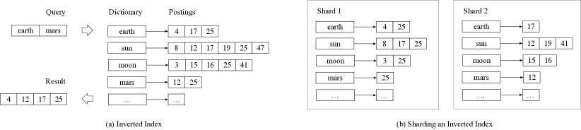
As highlighted in Figure 1 (a), in its simplest form, an inverted index is usually composed of terms that point to collections of document identifiers called postings lists [21]. Boolean queries can then be used to retrieve all the documestnts that contain a set of words. Optionally, a posting list can also contain the position of the term in the document. This positional information can then be used to search for sub-sequences in documents. However, when searching for long sub-sequences of terms, this approach showcases poor performances. In the context of trajectory indexing, we replace the terms of the inverted index with features, called geodabs, extracted from trajectories.

II-A2 Ranked Retrieval

In ranked retrieval, many records match with the query specified by the user, and it is common to rank the results according to a similarity measure. Therefore, the user can begin by considering the most relevant results and then decide to retrieve the remaining ones if necessary. In the context of textutal data, the union and the intersection of two sets of words $F$ and $G$ can be used to derive relevant similarity measures. For example, the Jaccard coefficient $J(F,G)$ is commonly used to gauge the similarity between texts and rank results [21]. Interestingly, the Jaccard distance $d_{J}(F,G)$ expressed in Equation 1 is complementary to the Jaccard coefficient and is proven to obey the triangular inequality [17]. Therefore, this distance can be used in conjunction with an index of pre-computed distances to efficiently prune candidates. In our context, we use the Jaccard distance to implement function $\delta(S_{q},S_{j})$ and rank the trajectories retrieved from the inverted index.

$$d_{J}(F,G)=1-J(F,G)=1-{{|F\cap G|}\over{|F\cup G|}}$$ (1)

II-A3 Normalization

It is worth noting that, in many cases, terms can be different but convey similar semantics or meaning. In general, the process of mitigating these differences is referred to as normalization [21]. For example, a common normalization technique consists in using equivalence classes for synonyms. In the context of trajectory indexing, we refer to normalization as a function $N(S)=S^{\prime}$, where $S$ and $S^{\prime}$ are sequences of points.

II-A4 Sharding

When an index becomes very large, it might not fit on a single computer anymore. As illustrated in Figure 1 (b), sharding the index across the nodes of a cluster becomes necessary. Here, the idea is to route documents to specific shards in order to spread the load throughout the cluster. At query time, all the shards might need to process a query to compute the result. Therefore, given the terms specified in a query, a good sharding strategy tries to minimize the number of shards that need to be contacted. Our solution effectively addresses this issue.

II-B Fingerprinting

As mentioned in Section II-A1, searching for long sub-sequences in textual data by using words and positional information is not very efficient. In practice, an inverted-index aimed at searching for sub-sequences is usually populated with a different class of terms, referred to as fingerprints [3, 20, 15, 2]. Fingerprints usually correspond to a sub-set of the hash sums obtained by hashing the n-grams of a document [25]. A n-gram is a sequence of $n$ contiguous items, i.e., $n$ words in the context of textual data. A fingerprint usually corresponds to the hash sum $h\in\mathbb{R}$ obtained by hashing a n-gram. As the number of n-grams for a given text can be very large, a common practice consists in retaining the subset of fingerprints that satisfy the condition $h\bmod p=0$, where $p$ is a fixed sampling constant. The extracted fingerprint can then be used as terms in the inverted index. Furthermore, given two sets of fingerprints, their similarity can easily be derived by the Jaccard coefficient. In our context, we refer to fingerprinting as a function $W(S)=F$, where $S$ is a trajectory and $F$ is an ordered set of fingerprints.

II-C Geohashing

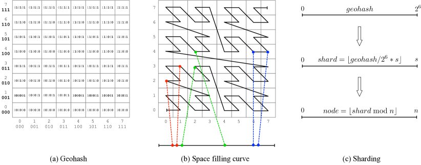
A function that produces geohashes maps a point $p$ to a sequence of bits $b$ that repeatedly bisect space up to a desired depth $d$ that defines the precision of the geohash [23]. In the case of a latitude/longitude space, the first subdivision usually occurs on the longitude axis, the second on the latitude axis and the process is repeated up to depth $d$. Figure 2 (a) illustrates this subdivision for a depth $d=6$, where two interleaved sequences of three bits are respectively dedicated to the subdivision of the longitude and latitude axes. Every geohash covers a delimited area on earth and, given a set of points $\{p_{1},p_{2},...,p_{n}\}$, it is relatively easy to find the highest precision geohash that overlaps with the whole set. Hereafter, we formally refer to such an overlapping geohash with the function $geohash(\{p_{1},p_{2},...,p_{n}\})=b$.

As highlighted in Figure 2 (b), the ordered list of hashes obtained by subdividing the space with a geohash function can be represented as a z-order space-filling curve. Interestingly, when two points are close to each other on a space-filling curve, then they are close to each other in the latitude/longitude space. However, the reverse is not necessarily true since: two points near each other in the latitude/longitude space might be far from each other on the space-filling curve.

Then, as illustrated in Figure 2 (c), the space-filling curve can be used to shard a spatial index across the nodes of a cluster. Two steps characterize the sharding strategy pictured here. First, geohashes are mapped to shards in a locality preserving way, i.e., geohashes near each other on the space-filling curve are placed on the same shard. Second, the shards are mapped to nodes with a modulo operation that breaks locality to improve the balance of the index across the nodes.

III Evaluation

Figure 3: Routes used to generate the trajectory dataset

Figure 4: Similar trajectories extracted form the dataset

Figure 5: Verifying configuration parameters with a PR curve

Figure 6: Increasing the number
of trajectory candidates

Figure 7: Increasing the length
of the trajectory candidates

In this section, we highlight the cost of computing distances and discovering motifs with DFD, DTW and Jaccard in dense trajectory datasets. To this aim, we characterize a large synthetic datasets and the configuration parameters we used to perform our evaluation. Our experiments confirm the pragmatic observation made in section and enable us to focus on Jaccard based methods. We then compare geodabs with geohashes, both in term of efficiency and effectiveness on a large and dense trajectory dataset. Finally, we evaluate how a geodab index can be sharded across a set of nodes.

III-A Evaluation Setup

III-A1 Datasets

To perform our evaluation, we extensively rely on a synthetic dataset and on the road network extracted from the OpenStreetMap dataset [14]. In the context of trajectory indexing, we noticed a lack of large and dense trajectory datasets. For example, the Nokia and Geolife datasets [18, 29] are too small and too sparse to validate our contributions. In addition, these datasets lack the trajectory queries and the associated ground truth that is required to qualitatively assess our solution. These kinds of queries and ground truths, also lack in the popular BerlinMod synthetic dataset [8]. Therefore, we used the trajectory generator introduced in [6] to create a synthetic dataset, a set of trajectory queries and the associated ground truth.

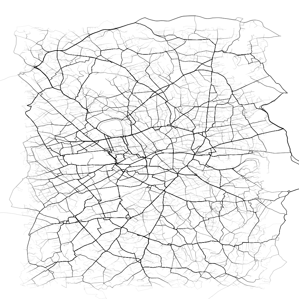
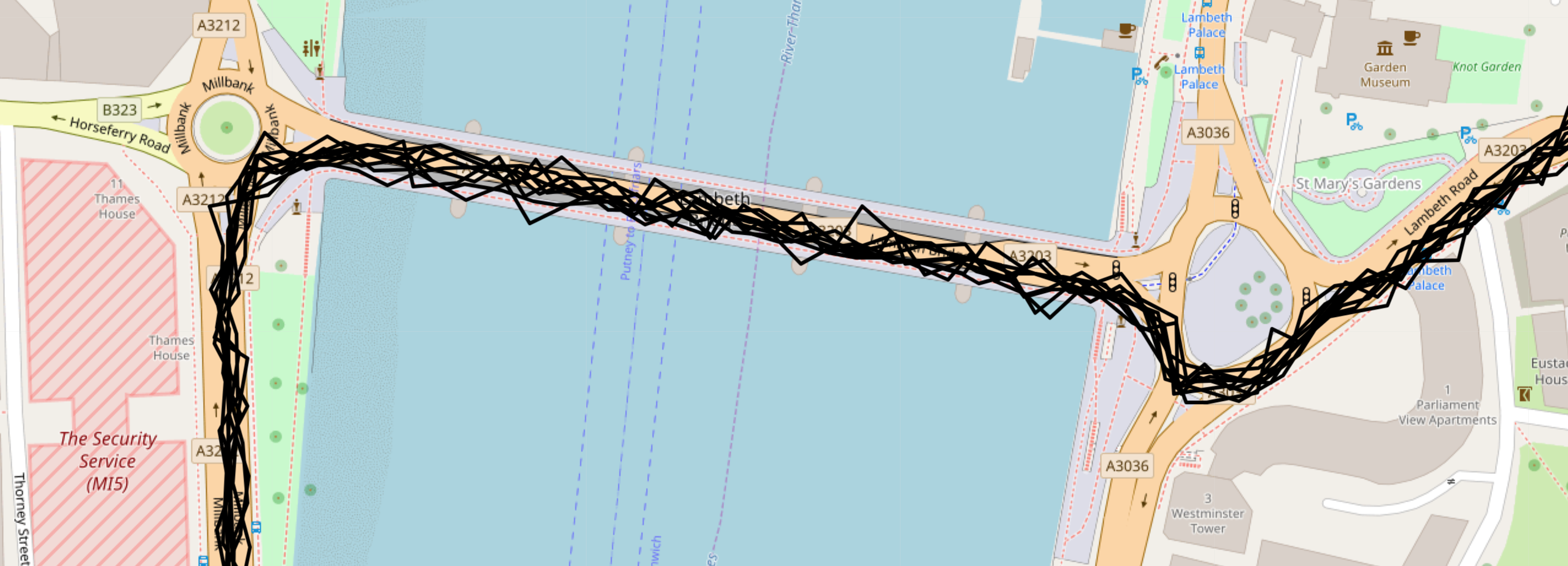
Our dataset is based on 5’000 unique routes constrained on a road network and generated with the GraphHopper library [16]. The routes are all located in a dense area of $300$ square kilometres located around the center of London. We use these routes to generate $10$ similar trajectories in one direction and $10$ similar trajectories in the opposite direction. These trajectories are sampled uniformaly at a rate of one point every second. The speed of the moving entities is based on the route duration computed by the GraphHopper library. In addition, we add $20$ meters of random Gaussian noise to every sampled points to make the dataset more realistic.

Figure 3 visually depicts the $5^{\prime}000$ routes used to generate the trajectory dataset. The $100^{\prime}000$ trajectories derived from these routes form a very dense dataset of $6.3Gb$ that mimics the traces GPS trackers would record. As of today, we found no publicly available counter parts to this synthetic dataset. However, we believe that additional work on the generation of a dense trajectory dataset would greatly benefit the research community. Figure 4 illustrates a set of $10$ similar trajectories generated on the basis of a route constrained to the road network.

III-A2 Configuration Parameters

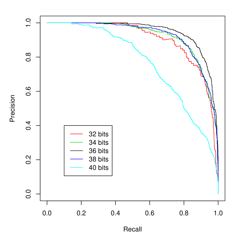
In order to evaluate the effectiveness of our solution, we need to find appropriate configuration parameters. First, we empirically evaluated several configurations and observed the best results with a normalization based on geohashes of $36$ bits, a lower bound of $k=6$ and an upper-bound of $t=12$. As we get closer to the poles, the width of the geohashes tends to shrink. In London, a geohash of $36$ bits has a width of $95$ meters and a height of $76$ meters. As a trajectory normalized with geohashes rarely follows a diagonal path, we can assume that the average length of a move between two geohashes is approximately $85$ meters. Therefore, the lower-bound $k$ translates to a segment threshold of approximately $510$ meters. Segments shorter than this threshold are considered as noise. The upper-bound $t$ translates to a segment threshold of approximately $1020$ meters. Segments greater than this threshold are guaranteed to be detected. To validate our parameters, we tested several levels of normalization, performed queries on a sample of our dataset and plotted the corresponding precision and recall curves. As highlighted in Figure 7, the normalization based on geohashes of $36$ bits clearly outperform its upstream and downstream counterparts. Automating the discovery of the appropriate parameters is a difficult task, because the number of possible combinations is very large and each configuration requires building and querying an index. A hill-climbing strategy could probably be used to address this problem, and this might be part of our future work.

III-B The Cost of Computing Distances

In this section, we characterize the cost of computing distances between trajectories and discuss their limits when searching trajectories in dense datasets. We begin by reminding some fundamental distance measures. We then compare them with the Jaccard distance used in the context of our paper.

III-B1 Ground Distance

Equation 2 describes the haversine ground distance formula, where $R$ corresponds to the earth’s radius in meters. Given a pair of points $p_{l}=(\varphi_{l},\lambda_{l})$ and $p_{k}=(\varphi_{k},\lambda_{k})$, the resulting value in $d(p_{l},p_{k})$ corresponds to the ground distance in meters.

$$2R\arcsin{\sqrt{\sin^{2}\left({\frac{\varphi_{l}-\varphi_{k}}{2}}\right)+\cos(\varphi_{k})\cos(\varphi_{l})\sin^{2}\left({\frac{\lambda_{l}-\lambda_{k}}{2}}\right)}}$$ (2)

III-B2 Dynamic Time Warping

Equation 3 presents the recursive function used to compute the dynamic time-warping distance (DTW) [28]. Given a trajectory $P=\langle p_{1},...,p_{m}\rangle$ and a trajectory $Q=\langle q_{1},...,q_{n}\rangle$, the resulting value in $dtw(|P|,|Q|)$ corresponds to the DTW distance between the trajectories.

$$dtw(i,j)=\begin{cases}\infty&\text{if $i=0$ or $j=0$}\\ 0&\text{if $i=j=0$}\\ d(P_{i},Q_{j})+min\begin{cases}dtw(i-1,j)\\ dtw(i,j-1)\\ dtw(i-1,j-1)\end{cases}&\text{otherwise}\end{cases}$$ (3)

III-B3 Discrete Fréchet Distance

Similarly, Equation 4 describes the recursive function used to compute the discrete Fréchet distance (DFD) [9]ite. The resulting value in $dfd(|P|,|Q|)$ also corresponds to the DFD distance between the trajectories.

$$dfd(i,j)=\begin{cases}d(P_{i},Q_{j})&\text{if $i=j=1$}\\ max\begin{cases}d(P_{i},Q_{j})\\ min\begin{cases}dfd(i-1,j)\\ dfd(i,j-1)\\ dfd(i-1,j-1)\end{cases}\end{cases}&\text{otherwise}\end{cases}$$ (4)

III-B4 Performance Evaluation

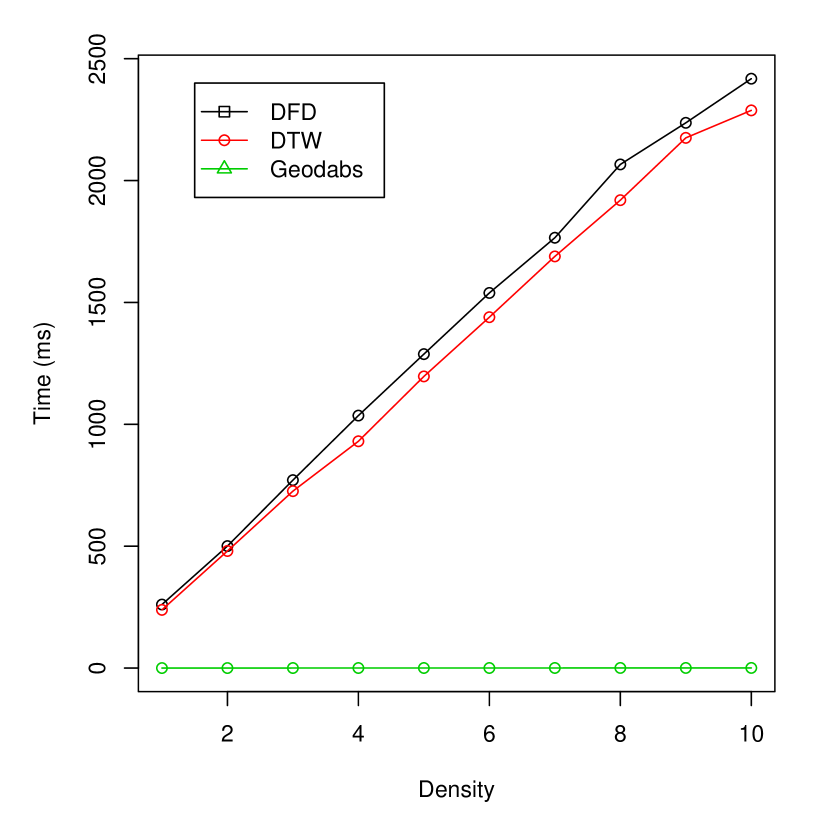
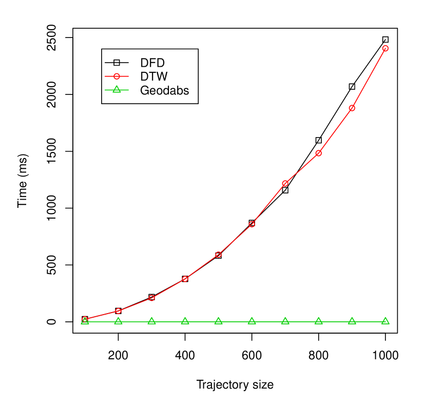
We compute the distance between a single query trajectory of length $t$ and a set of trajectory candidates of size $c$, where each candidate has a length of $t$. In such a scenario, the computational cost associated with the computation of DTW and DFD is characterised by a complexity of $O(c*t^{2})$. In Figure 7, the size of the set of trajectory candidates $c$ remains constant, and the length of the query and candidate trajectories increases. As highlighted here, as the length of the trajectories increases, so does the computational time in a polynomial manner. Therefore, when a dataset is primarily made of long trajectories recorded at a high sampling rate, computing DTW or DFD is impractical. In Figure 7, the size of the set of trajectory candidates $c$ densifies and the length of the trajectories $t$ remains constant. As the size of the of the candidate set increases, so does the computational time in a linear manner. In both cases, we notice that computing the scores associated with $10$ trajectories of $1^{\prime}000$ points takes more than $2500$ milliseconds. In the context of a very dense trajectory dataset, a query can return many more relevant trajectory candidates, for which a distance measure still has to be computed.

Therefore, it is obvious that relying on these distance measures might be qualitatively sound but clearly unsustainable at scale. In contrast, as highlighted in Figures 7 and 7, computing the Jaccard distance for ordered sets of geodabs extracted from the trajectories is very inexpensive. This clearly confirms the correctness of the pragmatic observation made in section 7.

Figure 8: Motif discovery with increasing trajectory candidates

Figure 9: PR curve

Figure 10: ROC curve

III-C The Cost of Discovering Motifs

In order to find motifs in pairs of trajectories with geodabs, we have to make some assumptions regarding the normalization step. First, we use our dataset to estimate the average number of fingerprints extracted per meters $a$ from normalized trajectories. As a result, when looking for motifs of length $l$, we can translate this length to a number of fingerprints $f=l*a$. Therefore, given two ordered sets of geodabs $F_{i}$ and $F_{j}$ obtained by fingerprinting the trajectories $S_{i}$ and $S_{j}$, the problem now consists in returning a pair of motifs $(\bar{F}_{i},\bar{F}_{j})$ such that $\mathit{length}(\bar{F}_{i})=\mathit{length}(\bar{F}_{j})=f~{}\wedge\not\exists(\bar{F^{\prime}}_{i},\bar{F^{\prime}}_{j})$ for which $d_{J}(\bar{F^{\prime}}_{i},\bar{F^{\prime}}_{j})~{}<~{}d_{J}(\bar{F}_{i},\bar{F}_{j})$. As the ordered sets $F_{i}$ and $F_{j}$ are usually relatively small, a brute force implementation of this method gives good results. Because of the normalization and the fingerprinting, the motifs discovered with this approach are not strictly equivalent in terms of length and are subject to threshold effects. However, the results we observed in practice are good approximations of the best result.

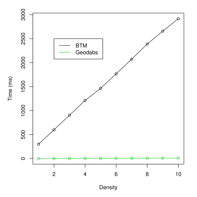
In Figure 10, we compare our method with an optimized algorithm, called bounding-based trajectory motif (BTM), which gives exact solutions to the motif-discovery problem by computing DFD for every motif pair in the trajectories [27]. As illustrated here, as the number of trajectory candidates densifies, so does the computational time. Again, our method based on geodabs appears to be a necessary tradeoff.

III-D The Cost of Indiscrimination

An inability of the index to discriminate between true and false positive translates to a greater set of trajectories for which the distance has to be computed. In this section, we characterize the effectiveness and the probabilistic nature of the geohash and geodabs indexes. We then show how an inability to discriminate directly affects performances.

Figure 11: Executing 100 queries on a large dataset of increasing density

Figure 12: Distribution of the trajectories
in geohash areas

Figure 13: Distribution of the trajectories
in a 10 nodes cluster

III-D1 Index Effectiveness

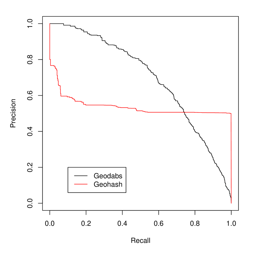
Figure 10 depicts the PR curves obtained by querying the geodabs and geohash indexes [21]. When looking at the geohash curve, we first notice that precision drops rapidly as recall increases. This is due to the inability of the geohash index to discriminate among similar trajectories that go in opposite directions. Because each trajectory of our synthetic dataset is associated with a return path, the geohash curve tends to stabilise at a precision of $0.5$, as recall increases. The curve associated with the geodab index clearly shows that our method addresses this discrimination issue. Furthermore, we also notice that the first results returned by the geodab index are characterized by very high precision. In the context of a very dense dataset, this property is desirable because we can focus on the subset of the most relevant results.

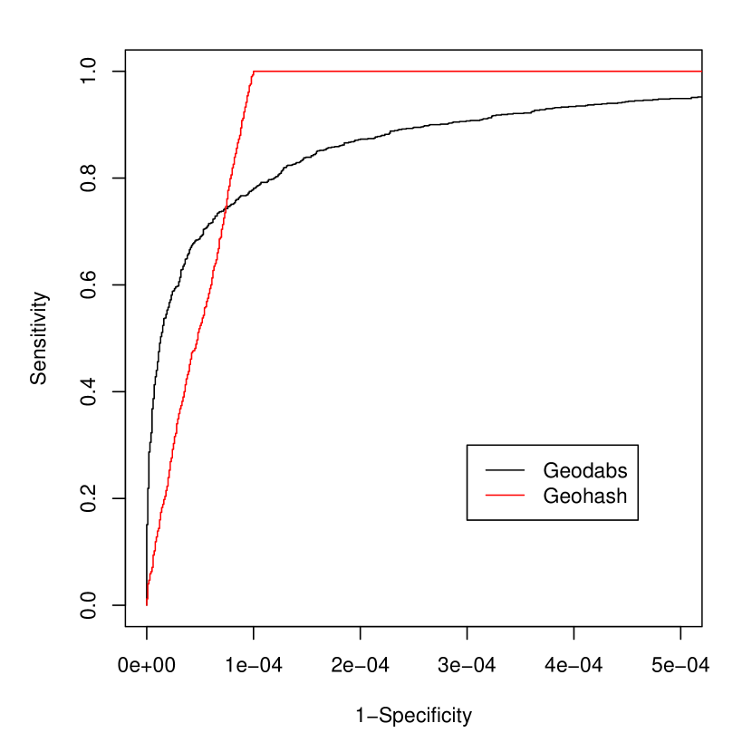
Figure 10 depicts the receiver-operating-characteristics (ROC) curve obtained by querying the geodab and geohash indexes [10]. In ranked retrieval, sensitivity usually corresponds to recall and specificity is given by $tn/(fp+tn)$. Thus, in contrast with the PR curve, the ROC curve enables us to qualitatively assess the full retrieval spectrum [21]. As we look at the full retrieval spectrum, the quality our results is exacerbated by the size of the dataset. Therefore, it is important to notice that the plot focuses on a very narrow interval of the specificity. In fact, qualitatively speaking, both indexes are characterized by a very high sensitivity and a marginally low number of relevant results are lost. This is confirmed by computing the area under the ROC curve (AUC) that is of $0.999889$ for geodabs and $0.9999521$ for geohashes. Here, the minor difference in terms of AUC comes from the fact that a marginal number of relevant results can be missed with geodabs. the fact that the curve associated with geodabs climbs more steeply, however, confirms that the first results returned by our method are more relevant.

III-D2 Index Efficiency

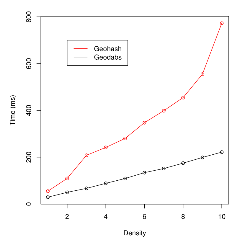
Figure 13 compares the average time needed to process $100$ queries on inverted indexes built with a sample of up to $10^{\prime}000$ trajectories. Here, in contrast with the results highlighted in Section III-B, the number of trajectory candidates is not controlled. Therefore, the difference between geohash and geodabs mainly highlights the inability of geohash to discriminate among trajectories. By combining several cells into one hash, a geodab not only discriminates on the direction of the trajectory, but also by all its constituents. Therefore, the number of candidates for which the Jaccard distance has to be computed is significantly reduced. As a result, processing queries is significantly faster but as shown earlier, the quality is not compromised.

III-E The Distribution of the Index

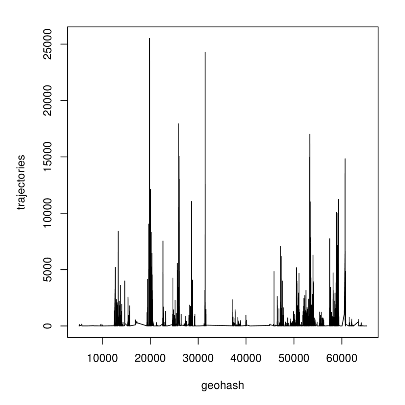
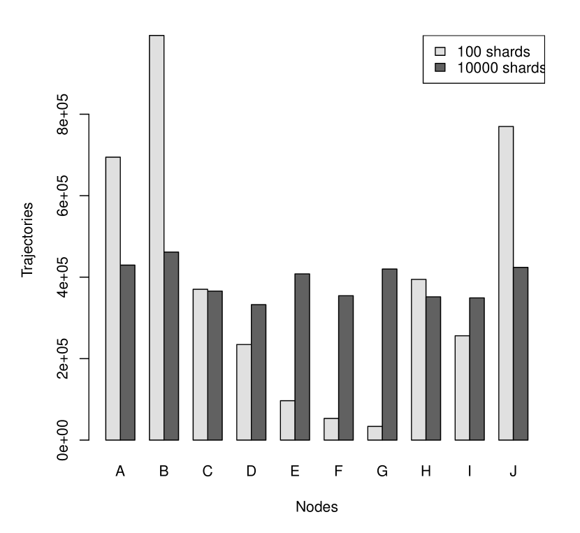
We test the distributed nature of our index with a global road network extracted from the full dump of OpenStreetMap. Here, we make the assumption that the distribution of trajectories recorded across the world should mostly fit on a road network and be characterized by a similar distribution. The geodabs produced by our algorithm are characterized by a geohash prefix of $16$ bits that can easily be extracted with a bitwise operation. Geohashes of depth $16$ subdivide space into $2^{16}$ cells characterized by a width of approximately 156 kilometres at the equator. In Figure 13, we plot the number of trajectories per geohash and we notice some very dense areas. For example, the highest peak located on the left of the diagram corresponds to the geohashes located around Mexico city. In contrast, the voids we have between the peaks correspond to areas of low activity, such as oceans. In Figure 13, we assume that the index is distributed across $10$ nodes. We notice that a small number of shards ($100$) is not sufficient to distribute the data in a balanced fashion. However, with a greater number of shards ($10^{\prime}000$), the data are well balanced on the nodes. Therefore, there is a tradeoff to make between preserving locality (to reduce the number of shards contacted when performing queries) and breaking locality (to spread the data evenly in the the cluster).

IV Conclusion

In this paper, we have shown that fingerprinting, and more specifically winnowing, can be used for indexing trajectories. We have introduced geodabs, a construction that combines hashing and geohashing to discriminate on the spatial and on the temporal dimensions. In addition, we have shown that geodabs can be used to scale and distribute an index across several nodes in a cluster. We have demonstrated how trajectory normalization can be used to improve the quality of an index. Finally, we discussed several pragmatic experiments that demonstrated the effectiveness and efficiently of trajectory fingerprinting with geodabs.

References

- [1] J. L. Bentley. Multidimensional binary search trees used for associative searching. Communications of the ACM, 18(9):509–517, 1975.
- [2] S. Brin, J. Davis, and H. Garcia-Molina. Copy detection mechanisms for digital documents. In ACM SIGMOD Record, volume 24, pages 398–409. Acm, 1995.
- [3] A. Z. Broder. On the resemblance and containment of documents. In Compression and Complexity of Sequences 1997. Proceedings, pages 21–29. IEEE, 1997.
- [4] V. P. Chakka, A. C. Everspaugh, and J. M. Patel. Indexing large trajectory data sets with seti. Ann Arbor, 1001(48109-2122):12, 2003.
- [5] B. Chapuis, P. Andritsos, and B. Garbinato. An efficient type-agnostic approach for finding sub-sequences in data. In Data Science and Systems (DSS), 2017 3rd International Conference on. IEEE, 2017.
- [6] B. Chapuis and B. Garbinato. Scaling and load testing location-based publish and subscribe. In Distributed Computing Systems (ICDCS), 2017 IEEE 37th International Conference on, pages 2543–2546. IEEE, 2017.
- [7] P. Dewan, R. Ganti, and M. Srivatsa. Som-tc: Self-organizing map for hierarchical trajectory clustering. In Distributed Computing Systems (ICDCS), 2017 IEEE 37th International Conference on, pages 1042–1052. IEEE, 2017.
- [8] C. Düntgen, T. Behr, and R. H. Güting. Berlinmod: a benchmark for moving object databases. The VLDB Journal—The International Journal on Very Large Data Bases, 18(6):1335–1368, 2009.
- [9] T. Eiter and H. Mannila. Computing discrete fréchet distance. Technical report, Tech. Report CD-TR 94/64, Information Systems Department, Technical University of Vienna, 1994.
- [10] T. Fawcett. Roc graphs: Notes and practical considerations for researchers. Machine learning, 31(1):1–38, 2004.
- [11] R. A. Finkel and J. L. Bentley. Quad trees a data structure for retrieval on composite keys. Acta informatica, 4(1):1–9, 1974.
- [12] C. Y. Goh, J. Dauwels, N. Mitrovic, M. T. Asif, A. Oran, and P. Jaillet. Online map-matching based on hidden markov model for real-time traffic sensing applications. In Intelligent Transportation Systems (ITSC), 2012 15th International IEEE Conference on, pages 776–781. IEEE, 2012.
- [13] A. Guttman. R-trees: A dynamic index structure for spatial searching, volume 14. ACM, 1984.
- [14] M. Haklay and P. Weber. Openstreetmap: User-generated street maps. IEEE Pervasive Computing, 7(4):12–18, 2008.
- [15] N. Heintze et al. Scalable document fingerprinting. In 1996 USENIX workshop on electronic commerce, volume 3, 1996.
- [16] P. Karich and S. Schröder. Graphhopper. http://www.graphhopper.com, last accessed, 4(2):15, 2014.
- [17] S. Kosub. A note on the triangle inequality for the jaccard distance. arXiv preprint arXiv:1612.02696, 2016.
- [18] J. K. Laurila, D. Gatica-Perez, I. Aad, O. Bornet, T.-M.-T. Do, O. Dousse, J. Eberle, M. Miettinen, et al. The mobile data challenge: Big data for mobile computing research. In Pervasive Computing, number EPFL-CONF-192489, 2012.
- [19] D. Lemire, O. Kaser, N. Kurz, L. Deri, C. O’Hara, F. Saint-Jacques, and G. Ssi-Yan-Kai. Roaring bitmaps: Implementation of an optimized software library. arXiv preprint arXiv:1709.07821, 2017.
- [20] U. Manber et al. Finding similar files in a large file system. In Usenix Winter, volume 94, pages 1–10, 1994.
- [21] C. D. Manning, P. Raghavan, and H. Schütze. Introduction to Information Retrieval. Cambridge University Press, New York, NY, USA, 2008.
- [22] P. Newson and J. Krumm. Hidden markov map matching through noise and sparseness. In Proceedings of the 17th ACM SIGSPATIAL international conference on advances in geographic information systems, pages 336–343. ACM, 2009.
- [23] G. Niemeyer. Geohash, 2008.
- [24] D. Pfoser, C. S. Jensen, Y. Theodoridis, et al. Novel approaches to the indexing of moving object trajectories. In VLDB, pages 395–406, 2000.
- [25] S. Schleimer, D. S. Wilkerson, and A. Aiken. Winnowing: local algorithms for document fingerprinting. In Proceedings of the 2003 ACM SIGMOD international conference on Management of data, pages 76–85. ACM, 2003.
- [26] M. Srivatsa, R. Ganti, and P. Mohapatra. On the limits of subsampling of location traces. In Distributed Computing Systems (ICDCS), 2017 IEEE 37th International Conference on, pages 1032–1041. IEEE, 2017.
- [27] B. Tang, M. L. Yiu, K. Mouratidis, and K. Wang. Efficient motif discovery in spatial trajectories using discrete fréchet distance. EDBT, 2017.
- [28] B.-K. Yi, H. Jagadish, and C. Faloutsos. Efficient retrieval of similar time sequences under time warping. In Data Engineering, 1998. Proceedings., 14th International Conference on, pages 201–208. IEEE, 1998.
- [29] Y. Zheng, X. Xie, and W.-Y. Ma. Geolife: A collaborative social networking service among user, location and trajectory. IEEE Data Eng. Bull., 33(2):32–39, 2010.