Survival of a planet in short-period Neptunian desert under effect of photo-evaporation

Abstract

Despite the identification of a great number of Jupiter-like and Earth-like planets at close-in orbits, the number of “hot Neptunes” — the planets with 0.6–18 times of Neptune mass and orbital periods less than 3 days — turned out to be very small. The corresponding region in the mass-period distribution was assigned as the “short-period Neptunian desert”. The common explanation of this fact is that the gaseous planet with few Neptune masses would not survive in the vicinity of host star due to intensive atmosphere outflow induced by heating from stellar radiation. To check this hypothesis we performed numerical simulations of atmosphere dynamics for a hot Neptune. We adopt the previously developed self-consistent 1D model of hydrogen-helium atmosphere with suprathermal electrons accounted. The mass-loss rates as a function of orbital distances and stellar ages are presented. We conclude that the desert of short-period Neptunes could not be entirely explained by evaporation of planet atmosphere caused by the radiation from a host star. For the less massive Neptune-like planet, the estimated upper limits of the mass loss may be consistent with the photo-evaporation scenario, while the heavier Neptune-like planets could not lose the significant mass through this mechanism. We also found the significant differences between our numerical results and widely used approximate estimates of the mass loss.

1 Introduction

The epoch of exoplanet observations and discoveries started more than twenty years ago. Over this time, more than 3600 exoplanets in about 2700 systems have been identified. The current observational methods allow not only to detect an exoplanet and to get its orbital characteristics but also to inspect parameters of its atmosphere (Seager, 2010). The observations of transits and anti-transits as well as direct observations of exoplanets made it possible to obtain the spectra of their upper atmospheres (Vidal-Madjar et al., 2003; Vidal-Madjar et al., 2004; Linsky et al., 2010; Janson et al., 2010; Barman et al., 2011). These spectra, in turn, can be used to determine the chemical and physical structure of exoplanet atmospheres as well as their dynamics.

Up to now, the most powerful methods of detecting exoplanets are the transit and radial velocity methods. Both are more effective to identify exoplanets which are close to their host stars. Therefore, it is natural that initially discovered exoplanets turned out to have close-in orbits. Until recently, the most of known planets belongs to “hot Jupiters” — exoplanets with masses that are comparable to Jupiter’s and orbital distances less than 0.1 AU (Murray-Clay et al., 2009). Thanks to the Kepler Space Telescope, it became possible to detect “super-Earths” — exoplanets with several Earth masses.

The further analysis of the discovered planet parameters has revealed an interesting feature. Despite the identification of great number of Jupiter-like and Earth-like planets at close-in orbits, the number of “hot Neptunes” — planets with 0.6–18 times of Neptune mass and orbital periods less than 3 days — turned out to be very small. The corresponding region in the mass-period distribution was assigned as the “short-period Neptunian desert” (Szabó & Kiss, 2011; Howe & Burrows, 2015; Mazeh et al., 2016). This region can be hardly explained by selection effects. Indeed, the adopted methods potentially are more sensitive to more massive planets. While being successful for identification of super-Earths they should be even more effective for detecting the short-period Neptunes at the same orbits. Hence, the desert of short-period Neptunes has likely the physical origin. The more detailed analysis of the selection effects and their relation to the problem of short-period Neptunes can be found in Mazeh et al. (2016), where the functional expression to describe the upper and lower boundary of the short-period Neptune desert in the mass-period diagram was also provided. According to their data, the upper boundary is represented by the relation $M_{p}(M_{J})=P^{-1.14\pm 0.14}\cdot 10^{0.23\pm 0.045}$ while the lower boundary can be expressed as $M_{p}(M_{J})=P^{0.98}\cdot 10^{-1.85}$, where $P$ is the orbital period evaluated in days. To explain the origin of the desert the following hypotheses were mentioned in  Mazeh et al. (2016):

1. During the protoplanetary evolution the planet migrates toward the star from the external parts of protoplanetary disk. This migration driven by the interaction with the disk stopped near the inner edge of the disk where the density is too low to continue pushing the planet inward. It is suggested that the inner disk radius depends on the disk mass being smaller for more massive disks. Thus, the more massive planets are presumably formed in more massive disks and settle on smaller orbital distances.

2. The gaseous planets with Neptune masses would not survive in the vicinity of host star due to intensive atmosphere outflow caused by stellar radiation.

The second hypothesis is considered in Kurokawa & Nakamoto (2014); Kurokawa & Kaltenegger (2013); Tian (2015). The same process is observed toward other exoplanets as well. Orbiting close to their parent stars, the exoplanets with H/He-dominant envelopes are exposed to an integrated high-energy irradiation that is an appreciable fraction of their gravitational binding energy (Lammer et al., 2003; Tian et al., 2005). Such high-energy irradiation is typical for the first 100 Myr of the planet’s lifetime (Jackson et al., 2012). As a consequence, the H/He-dominant envelopes can be strongly evaporated by this irradiation (Tian et al., 2005; Owen & Jackson, 2012; Johnstone et al., 2015). Such strong H/He evaporation has been observed from the high-mass planets HD 209458b (Vidal-Madjar et al., 2003), HD189733b (Lecavelier Des Etangs et al., 2010), WASP-12b (Fossati et al., 2010a, b), and from the low-mass planet GJ 436b (Kulow et al., 2014; Ehrenreich et al., 2015). Evaporation naturally arises in planets that are smaller and denser than those at large separations (Lopez et al., 2012; Owen & Wu, 2013; Lopez & Fortney, 2013; Jin et al., 2014). For a planet with a low enough mass and a close enough orbit, its initial low-mass H/He envelope can even be entirely stripped, leaving behind a naked solid core. The core’s mass and density play an important role in controlling a planet’s evolution by setting the escape velocity (Owen & Wu, 2013; Lopez & Fortney, 2013; Owen & Morton, 2016; Zahnle & Catling, 2017).

The evaporation theory is very useful in the studies of the exoplanet demographics. It allows to infer the different populations of exoplanets. For instance, it predicted the existence of an “evaporation valley”, a low-residence region in the radius-period plane between planets that have been completely stripped and those that are able to retain their envelopes with roughly $\approx$1% in mass. The evaporation valley was firstly predicted by Owen & Wu (2013) using numerical evolutionary studies for low-mass planets with pure rock (silicate) cores, and shortly after, by Lopez & Fortney (2013) for various core compositions using a different evaporation model. This feature can be considered also as a radius valley, i.e. a bimodal distribution of planet radii, with super-Earths and sub-Neptune planets separated by a valley at around $\approx 2R_{Earth}$. Such a valley was observed recently, owing to an improvement in the precision of stellar, and therefore planetary radii (Fulton et al., 2017; Van Eylen et al., 2017). The evaporation valley is thus a robust prediction of evaporative driven evolution of close-in H/He dominant planets (Owen & Wu, 2013; Lopez & Fortney, 2013; Jin et al., 2014; Chen & Rogers, 2016; Owen & Wu, 2017; López et al., 2017).

The photo-evaporation hypothesis is usually adopted to explain the upper boundary of the short period Neptunes desert. The theory designed to explain both upper and bottom boundaries has been presented in Matsakos & Königl (2016). They argue that the desert may appear in scenarios of the orbital circularization of planets that arrive at the stellar vicinity on high-eccentricity orbits and of their subsequent tidal angular-momentum exchange with the star.

In our paper, the study of the mass loss of a hot Neptune due to the hydrodynamical outflow from its atmosphere is presented. This outflow is induced by the heating of the atmosphere. The main heating mechanism is associated with the absorption of stellar XUV (soft X-rays and extreme ultraviolet) radiation, in particular, in the range of 1–100 nm (Lammer et al., 2003; Lammer et al., 2009; Shaikhislamov et al., 2014; Tian et al., 2005). This process was investigated in Kurokawa & Nakamoto (2014) where the authors simulated the atmosphere outflow with the 1D semianalytic evolutionary model of a sub-Jupiter. To calculate the mass loss due to stellar radiation they adopted the following formula from Lopez & Fortney (2014):

$$\frac{dM_{p}}{dt}=-\frac{\pi\eta F_{XUV}R^{3}_{XUV}}{GM_{p}K_{t}},$$ (1)

where $M_{p}$ is the planet mass, $F_{XUV}$ the incident XUV stellar flux, $R_{XUV}$ the radius (evaluated from the planet center) at which the XUV emission is absorbed, $K_{t}$ the coefficient to account for the tidal force from the star, and $\eta$ the heating efficiency. Using the obtained outflow rates and corresponding exoplanet lifetimes, Kurokawa & Nakamoto (2014) derived the upper boundary of short period Neptunes desert in period-mass diagram. With the adopted value of heating efficiency 0.25, the planets below the upper boundary should be evaporated in less than 2 Gyr. However, in our study Shematovich et al. (2014) it was shown that the mean value of heating efficiency is equal to 0.14 if the generation of suprathermal electrons is taken into account. Since the heating efficiency is an important parameter let us describe the heating of the atmosphere in more detail.

The XUV radiation causes the ionization of atomic hydrogen and helium, as well as the ionization, dissociation and dissociative ionization of molecular hydrogen (Shematovich, 2010; Shematovich et al., 2014; Ionov & Shematovich, 2015). These processes are described by the following equations:

$$\begin{array}[]{l}H_{2}+h\nu(e_{p})\rightarrow H_{2}^{+}+e_{p}+(e)\\ H_{2}+h\nu(e_{p})\rightarrow H(1s)+H(1s,2s,2p)+(e_{p})\\ H_{2}+h\nu(e_{p})\rightarrow H(1s,2p)+H^{+}+e_{p}+(e)\\ H+h\nu(e_{p})\rightarrow H^{+}+e_{p}+(e)\\ He+h\nu(e_{p})\rightarrow He^{+}+e_{p}+(e),\end{array}$$ (2)

where $h\nu$, $e_{p}$, $e$ are related to XUV-photon, photoelectron and secondary electron, correspondingly.

The fraction of absorbed photon energy provides ionization and dissociation while the remaining part is transferred into kinetic energy of the products, mainly, into kinetic energy of electrons. If the kinetic energy of the released photoelectron is high enough, i.e. when it is about ten times higher than local thermal energy (such electron is called suprathermal), this electron can stimulate the secondary ionizations and dissociations. At the same time, the suprathermal photoelectron can lose its energy during elastic collisions with other particles. Thus, the part of the photoelectrons energy goes into ionization and dissociation while the other part provides gas heating. Correspondingly, the consideration of processes with suprathermal electrons reduces the amount of energy which goes into heating, and thus significantly reduces the heating efficiency. Moreover, taking into account the suprathermal electrons the ionization rates will change as well, as shown in Ionov et al. (2014).

The goal of our paper is to check the possibility to explain the existence of short period Neptunes desert using the model of hydrodynamical outflow when appropriate processes with suprathermal electrons are taken into account. To answer this question we present the results of numerical simulations of hot Neptune atmosphere dynamics. We adopt the self-consistent model by Ionov et al. (2017) of hydrogen-helium atmosphere with suprathermal electrons accounted.

2 Model

Our model can be splitted into the kinetic, chemical, and hydrodynamical parts. Schematically, its structure is shown in Ionov et al. (2017) (Fig. 1, page 388). In the kinetic model, the heating intensity, as well as the ionization, dissociation, and excitation rates of the atmospheric species are calculated with the Monte Carlo model. The concentrations of the atmospheric species are calculated in the chemical model, based on the reaction rates evaluated in the kinetic model. Using the heating rates, the variations of atmospheric gas density, velocity, and temperature are provided by the gas-dynamical model.

The transport and kinetics of photoelectrons in planetary atmosphere were computed using the Monte Carlo model adopted from Shematovich (2008, 2010). This model includes the reactions (2) and the transport of suprathermal electrons. The energy of a secondary electron formed during a collision and subsequent ionization is chosen following the procedure described in Marov et al. (1996); Shematovich (2008, 2010).

With the Monte Carlo method, we compute the rate at which the energy of stellar XUV radiation and photoelectrons is transformed into the internal energy during the photoreactions and reactions with secondary electrons. Separately, we compute the energy of suprathermal photoelectrons that is transformed into the thermal energy. Using these rates the heating function of the atmosphere is calculated.

A system of chemical rate equations is solved in the chemical model. The chemical network includes 19 reactions involving nine components: H, H₂, e^-, H⁺, H${}_{2}^{+}$, H${}_{3}^{+}$, He, He⁺,and HeH⁺. The reaction rates were taken from García Muñoz (2007). One of the main channels for radiative cooling is the emission by H${}_{3}^{+}$ ion. To calculate the corresponded cooling function we take the temperature-dependent emissivity of H${}_{3}^{+}$ from Neale et al. (1996).

The gas-dynamical model is based on the numerical code described in Pavlyuchenkov et al. (2015). This 1D code was initially developed to compute the collapse of a protostellar cloud, and was adapted by us for a planetary atmosphere. The computations were carried out using Lagrangian grid, i.e. with moving cell boundaries. In our calculations, we used a grid that was non-uniform in the mass coordinate: the mass of the cell falls off with height as a geometric progression with factor 1.03. The artificial viscosity was introduced into the scheme in order to suppress oscillations arising in dense layers of the atmosphere. The value of this viscosity was chosen to be sufficient to suppress non-physical oscillations.

3 Model parameters

Our primary goal is to check the principal possibility for a hot Neptune to lose the most of its atmosphere due to the heating by stellar radiation. Therefore, our simulations were intended primarily to establish the upper limits for atmospheric mass loss rates. We also aim to compare our calculations with the estimates based on the approximate formula from Kurokawa & Nakamoto (2014).

In our previous paper Ionov et al. (2017), the gravitational potential was defined by a planet only. However, the outflowing atmosphere is extended and its dynamics can be affected by the host star as well. Indeed, the simulations by Bisikalo et al. (2013b); Bisikalo et al. (2013a) showed that the atmospheres of close-in gaseous planets overfill their Roch lobes that significantly increases the mass loss rate.

So, in this paper we use the approximate spherically-symmetric potential in the form of the Roche potential in the direction toward the $L_{1}$ point:

$$\Phi=-\frac{GM_{*}}{a-r}-\frac{GM_{p}}{r}-0.5\frac{G(M_{*}+M_{p})}{a^{3}}\left(r-\frac{M_{*}}{M_{*}+M_{p}}a\right)^{2},$$ (3)

where $a$ is the semi-major axis of the planet, $M_{*}$ is the stellar mass, and $M_{p}$ is the planet mass. This assumption does not recover the exact 3D nature of the Roche potential but is sufficient to obtain upper limits of mass loss since the outflow rate is highest toward the $L_{1}$ point. The same approach was adopted in García Muñoz (2007). In our calculations we assumed that stellar mass is equal to solar mass.

As was noted by Ribas et al. (2005), the intensity of XUV radiation of young solar-like stars could exceed the present solar intensity in 10–100 times. This should increase the corresponded mass loss rates and has to be taken into account. Thus, we perform our simulations using not only the solar spectrum but the spectra of young stars based on data from Ribas et al. (2005). Namely, we use approximate expressions to calculate the stellar radiation intensity at 1–20, 20–100, 100–360, 360–920, and 920–1180 Å  for the following stellar ages: 0.1, 0.3, 0.65, and 4.5 (present) billion years. The corresponding fluxes integrated over selected wavelength bands are shown in Fig. 1.

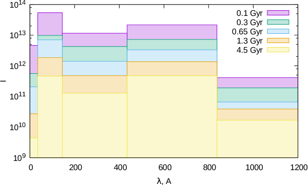
Figure 1: The stellar radiation fluxes integrated over selected wavelength bands. The distributions for different ages are shown with colors. The wavelength ranges are 1–20, 20–100, 100–360, 360–920 and 920–1180 Å.

Our calculations were performed for two cases of Neptune-like planets. The first model planet which we name “heavy” corresponds to the upper part of short-period Neptune desert and is six times heavier than Neptune, i.e. is equal to $6\times 10^{29}$ g. The second model planet assigned as “light” has the value of Neptune mass and represents the lower desert boundary. Note, that in the majority of previous studies the attention was paid presumably to upper desert boundary, see e.g. Kurokawa & Nakamoto (2014). The radii of both planets were calculated assuming their average densities to be the same as for Neptune. We have selected 0.05, 0.04, 0.03, and 0.02 AU for planet orbital distances. The positions of the considered models in the period-mass diagram, together with the parameters of the observed exoplanets and the estimated boundaries of Neptunian desert are shown in Fig. 2. Note, that the models with 0.04 and 0.05 AU correspond to the very edge of the Neptunian desert.

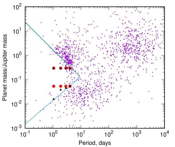
Figure 2: The observed exoplanet parameters extracted from exoplanet database at www.exoplanet.eu (blue dots), the initial (red circles) and final (black triangles) positions of the considered models in the period-mass diagram. The final model positions are calculated assuming that the planet matter was purely hydrogen-helium. The boundaries of short-period Neptunian desert are indicated by lines according to data from Mazeh et al. (2016).

4 Mass loss rate

Let us estimate the mass loss rate from approximate formula (1). One of the main parameters in formula (1) is the radius $R_{XUV}$ at which the XUV-radiation is absorbed. The exact value of this parameter is quite uncertain since the zone of effective XUV absorption is rather extended. Meanwhile, the mass loss rate in formula (1) is proportional to the third power of $R_{XUV}$ making the choice of $R_{XUV}$ important. Kurokawa & Kaltenegger (2013) suggested to use the radius where the intensity of XUV emission is reduced in $e$ times. Making this choice, however, the intensity at $R_{XUV}$ would depend on the incident stellar XUV flux. Alternatively, they used the relation $R_{XUV}=1.4R_{p}$, where $R_{p}$ is the planet radius. In the paper by Kurokawa & Nakamoto (2014) it was suggested to select $R_{XUV}$ as a radius at which the pressure is equal to $p=10^{-9}$ bar.

The mass loss rates estimated using approximate formula (1) and those calculated using our model are shown in Fig. 3. The left and right panels correspond to the light and heavy Neptune-like planets, respectively. The approximate rates calculated assuming $R_{XUV}=1.4R_{p}$ are shown with dashed lines. The solid lines correspond to the assumption that $R_{XUV}$ is the radius where the optical depth to XUV radiation is equal to unity. The optical depth is calculated based on the results of our simulations. For the case of light Neptune-like planet, the latter radius exceeds the former one (except for the age of 4.5 billion years when these radii are nearly the same). Thus, for the light planet, the approximate mass loss rates for the case $R_{XUV}=1.4R_{p}$ are lower than rates for $\tau(R_{XUV})=1$. For heavy planet the situation is opposite. The analytic estimates of mass loss rates were calculated with the heating efficiency $\eta=0.25$ as in Kurokawa & Nakamoto (2014).

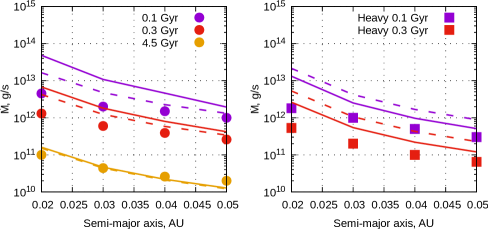
Figure 3: The mass loss rate as a function of the planet semi-major axis. The rates for different star ages are shown with different colors. The results for the light and heavy Neptune-like planets are given in the left and right panels, correspondingly. The simulated mass loss rates are shown with filled circles and boxes. The approximate rates calculated with formula (1) and assuming $R_{XUV}=1.4R_{p}$ are shown with dashed lines while the solid lines correspond to the case when $\tau(R_{XUV})=1$.

From the comparison between approximate curves and points estimated with our models one can figure out the following conclusion. For the star with present solar spectrum, the formula (1) provides a good fit to the results of numerical simulations. However, for the younger star the difference between approximate and calculated in our model rates becomes more significant. For the fixed stellar age, the difference becomes larger with the decrease of planet semi-major axis. Consequently, the approximate rates calculated with formula (1) are overestimated especially during the young stellar ages and closer-in planet orbits, i.e. in the cases when the mass loss rate is highest. This conclusion is valid both for the light and heavy cases of the considered Neptune-like planets.

Let us examine the question whether the calculated mass loss rates can cause a significant change in the planet mass. To calculate this, we have to take into account that the mass loss rate from a planet varies in time following the evolution of the stellar spectrum and luminosity. Given the limited number of calculated rates, we integrate the total mass loss $\Delta M$ with the approximate sum:

$$\Delta M=\sum_{i=1}^{5}\dot{M}_{i}\Delta t_{i},$$ (4)

where $\dot{M}_{i}$ is the mass-loss rate, corresponding to the i-th stellar XUV flux shown in Fig. 1, $\Delta t_{i}$ is its duration. Note, that this approach is rather crude and tends to overestimate the total mass loss.

First, let us consider the results obtained for the light Neptune-like planet model. Despite the fact that outflow rate estimated with our model is lower than that calculated with formula (1), it is still sufficient to cause a significant change of the planet mass. The important question here is the fraction of the hydrogen-helium envelope in the total mass of the planet. Under assumption that the hydrogen-helium envelope in the light Neptune-like planet model has the same mass as in Neptune, all the light planets placed in the short-period Neptunian desert will experience a complete loss of the envelope. If we assume that the envelope mass is 30% of the planet mass, the envelope will be completely evaporated for the orbits with periastris of 0.02 and 0.03 AU. However, the evaporation of the hydrogen-helium envelope does not mean that the planet escapes the short-period Neptunian desert. The planet still should get rid of a substantial fraction of mass (most probably stored in the water mantle). However, our model does not allow us to follow the evolution of planet after evaporation of the hydrogen-helium envelope. Therefore, the question whether the light Neptunes may survive in the short-period Neptunian desert requires further consideration.

In case of heavy Neptune-like planet the situation is more certain. The outflow rates are comparable to that of light planet. This is quite reasonable since the effect of larger planet surface is compensated by stronger gravitational acceleration. Being heavier, the planets lose only 5 % of the initial mass over first 1.5 billion years.

5 Conclusion

Based on the obtained results we conclude that the desert of short period Neptunes could not be reliably explained by the evaporation of planet atmospheres due to XUV radiation from host star.

While for the case of light Neptune-like planet, the calculated upper limits of the mass outflows are consistent with photo-evaporation scenario, in the case of heavy Neptune-like planets this mechanism does not allow to remove the significant fraction of the planet mass. Some other physical mechanisms like a high-eccentricity migration of planets that arrive in the vicinity of the Roche limit, where their orbits are tidally circularized, could be involved for the explanation of the upper boundary for the short-period Neptunian desert (Matsakos & Königl, 2016).

However, we must note that the calculated outflow rates are, in general, not fully consistent since we did not follow the evolution of the planet structure. It is necessary to take into account the change of mass and radius of the planet during the evaporation. The important effect is that a young planet may have much larger radius (than that for the evolved planet). Consequently, the young planet would be affected by stronger evaporation. These and other evolutionary effects are especially important in the case of a light Neptune-like planet where the outflow rates could be significant. We did not take these effects into account since our current approach to calculate the outflow rates is too computationally time consuming to be combined with such evolutionary model.

We did not consider a number of processes that could eventually increase the planet outflow rates. The first one is the flare activity of the host star. Indeed, during the star flares the stellar XUV intensity can be an order of magnitude higher than one in the quite state. As found by Glassgold et al. (2005), for solar-like star the duration of flashes is about $10^{5}$ sec, their X-ray intensity is 10 times higher than in quite state, and the interval between the flares is about 4–8 days. With the accounting of the stellar flares, the total XUV energy absorbed by a planet can be about three times higher than one considered in the quite conditions. According to formula (1) the outflow rate is proportional to XUV flux. Thus, the effect of flashes can be responsible for the “cleaning” of the bottom part of short period Neptune desert. However, this effect can not provide sufficient XUV fluxes to evaporate heavy Neptune-like planets i.e. to depopulate the top part of the desert.

Another factor that can be important is the coronal activity of the star. The influence of coronal mass ejections onto stability of a hot Jupiter atmosphere was studied in Bisikalo & Cherenkov (2016) and it was shown that the coronal mass ejection can stimulate the enhanced planet atmosphere loss. However, it is difficult for us to estimate this effect in case of hot Neptunes in frames of the adopted spherically symmetric model. One needs to use 3D hydrodynamical simulations to figure out if coronal mass ejection could significantly increase the rate of hot Neptune atmosphere evaporation.

6 Acknowledgements

We thank an anonymous referee for her/his suggestions that helped us to improve the quality of our paper. V. Shematovich acknowledges the support by the Russian Science Foundation (grant 18-12-00447).

References

- Barman et al. (2011) Barman T. S., Macintosh B., Konopacky Q. M., Marois C., 2011, ApJ, 733, 65
- Bisikalo & Cherenkov (2016) Bisikalo D. V., Cherenkov A. A., 2016, Astronomy Reports, 60, 183
- Bisikalo et al. (2013a) Bisikalo D. V., Kaigorodov P. V., Ionov D. E., Shematovich V. I., 2013a, Astronomy Reports, 57, 715
- Bisikalo et al. (2013b) Bisikalo D., Kaygorodov P., Ionov D., Shematovich V., Lammer H., Fossati L., 2013b, ApJ, 764, 19
- Chen & Rogers (2016) Chen H., Rogers L. A., 2016, ApJ, 831, 180
- Ehrenreich et al. (2015) Ehrenreich D., et al., 2015, Nature, 522, 459
- Fossati et al. (2010a) Fossati L., et al., 2010a, ApJ, 714, L222
- Fossati et al. (2010b) Fossati L., et al., 2010b, ApJ, 720, 872
- Fulton et al. (2017) Fulton B. J., et al., 2017, AJ, 154, 109
- García Muñoz (2007) García Muñoz A., 2007, Planet. Space Sci., 55, 1426
- Glassgold et al. (2005) Glassgold A. E., Feigelson E. D., Montmerle T., Wolk S., 2005, in Krot A. N., Scott E. R. D., Reipurth B., eds, Astronomical Society of the Pacific Conference Series Vol. 341, Chondrites and the Protoplanetary Disk. p. 165 (arXiv:astro-ph/0505562)
- Howe & Burrows (2015) Howe A. R., Burrows A., 2015, ApJ, 808, 150
- Ionov & Shematovich (2015) Ionov D. E., Shematovich V. I., 2015, Solar System Research, 49, 339
- Ionov et al. (2014) Ionov D. E., Bisikalo D. V., Shematovich V. I., Huber B., 2014, Solar System Research, 48, 105
- Ionov et al. (2017) Ionov D. E., Shematovich V. I., Pavlyuchenkov Y. N., 2017, Astronomy Reports, 61, 387
- Jackson et al. (2012) Jackson A. P., Davis T. A., Wheatley P. J., 2012, MNRAS, 422, 2024
- Janson et al. (2010) Janson M., Bergfors C., Goto M., Brandner W., Lafrenière D., 2010, ApJ, 710, L35
- Jin et al. (2014) Jin S., Mordasini C., Parmentier V., van Boekel R., Henning T., Ji J., 2014, ApJ, 795, 65
- Johnstone et al. (2015) Johnstone C. P., et al., 2015, ApJ, 815, L12
- Kulow et al. (2014) Kulow J. R., France K., Linsky J., Loyd R. O. P., 2014, ApJ, 786, 132
- Kurokawa & Kaltenegger (2013) Kurokawa H., Kaltenegger L., 2013, MNRAS, 433, 3239
- Kurokawa & Nakamoto (2014) Kurokawa H., Nakamoto T., 2014, ApJ, 783, 54
- Lammer et al. (2003) Lammer H., Selsis F., Ribas I., Guinan E. F., Bauer S. J., Weiss W. W., 2003, ApJ, 598, L121
- Lammer et al. (2009) Lammer H., et al., 2009, A&A, 506, 399
- Lecavelier Des Etangs et al. (2010) Lecavelier Des Etangs A., et al., 2010, A&A, 514, A72
- Linsky et al. (2010) Linsky J. L., Yang H., France K., Froning C. S., Green J. C., Stocke J. T., Osterman S. N., 2010, ApJ, 717, 1291
- Lopez & Fortney (2013) Lopez E. D., Fortney J. J., 2013, ApJ, 776, 2
- Lopez & Fortney (2014) Lopez E. D., Fortney J. J., 2014, ApJ, 792, 1
- Lopez et al. (2012) Lopez E. D., Fortney J. J., Miller N., 2012, ApJ, 761, 59
- López et al. (2017) López J. A., Richer M. G., Pereyra M., García-Díaz M. T., 2017, in Liu X., Stanghellini L., Karakas A., eds, IAU Symposium Vol. 323, Planetary Nebulae: Multi-Wavelength Probes of Stellar and Galactic Evolution. pp 352–353, doi:10.1017/S1743921317001879
- Marov et al. (1996) Marov M. Y., Shematovich V. I., Bisicalo D. V., 1996, Space Sci. Rev., 76, 1
- Matsakos & Königl (2016) Matsakos T., Königl A., 2016, ApJ, 820, L8
- Mazeh et al. (2016) Mazeh T., Holczer T., Faigler S., 2016, A&A, 589, A75
- Murray-Clay et al. (2009) Murray-Clay R. A., Chiang E. I., Murray N., 2009, ApJ, 693, 23
- Neale et al. (1996) Neale L., Miller S., Tennyson J., 1996, ApJ, 464, 516
- Owen & Jackson (2012) Owen J. E., Jackson A. P., 2012, MNRAS, 425, 2931
- Owen & Morton (2016) Owen J. E., Morton T. D., 2016, ApJ, 819, L10
- Owen & Wu (2013) Owen J. E., Wu Y., 2013, ApJ, 775, 105
- Owen & Wu (2017) Owen J. E., Wu Y., 2017, ApJ, 847, 29
- Pavlyuchenkov et al. (2015) Pavlyuchenkov Y. N., Zhilkin A. G., Vorobyov E. I., Fateeva A. M., 2015, Astronomy Reports, 59, 133
- Ribas et al. (2005) Ribas I., Guinan E. F., Güdel M., Audard M., 2005, ApJ, 622, 680
- Seager (2010) Seager S., 2010, Exoplanet Atmospheres: Physical Processes. Princeton University Press
- Shaikhislamov et al. (2014) Shaikhislamov I. F., Khodachenko M. L., Sasunov Y. L., Lammer H., Kislyakova K. G., Erkaev N. V., 2014, ApJ, 795, 132
- Shematovich (2008) Shematovich V. I., 2008, in Abe T., ed., American Institute of Physics Conference Series Vol. 1084, American Institute of Physics Conference Series. pp 1047–1054, doi:10.1063/1.3076436
- Shematovich (2010) Shematovich V. I., 2010, Solar System Research, 44, 96
- Shematovich et al. (2014) Shematovich V. I., Ionov D. E., Lammer H., 2014, A&A, 571, A94
- Szabó & Kiss (2011) Szabó G. M., Kiss L. L., 2011, ApJ, 727, L44
- Tian (2015) Tian F., 2015, Annual Review of Earth and Planetary Sciences, 43, 459
- Tian et al. (2005) Tian F., Toon O. B., Pavlov A. A., De Sterck H., 2005, ApJ, 621, 1049
- Van Eylen et al. (2017) Van Eylen V., Agentoft C., Lundkvist M. S., Kjeldsen H., Owen J. E., Fulton B. J., Petigura E., Snellen I., 2017, preprint, (arXiv:1710.05398)
- Vidal-Madjar et al. (2003) Vidal-Madjar A., Lecavelier des Etangs A., Désert J.-M., Ballester G. E., Ferlet R., Hébrard G., Mayor M., 2003, Nature, 422, 143
- Vidal-Madjar et al. (2004) Vidal-Madjar A., et al., 2004, ApJ, 604, L69
- Zahnle & Catling (2017) Zahnle K. J., Catling D. C., 2017, ApJ, 843, 122