Angle-Based Shape Determination Theory of Planar Graphs with Application to Formation Stabilization (Extended Version)

Abstract

This paper presents an angle-based approach for distributed formation shape stabilization of multi-agent systems in the plane. We develop an angle rigidity theory to study whether a planar framework can be determined by angles between segments uniquely up to translations, rotations, scalings and reflections. The proposed angle rigidity theory is applied to the formation stabilization problem, where multiple single-integrator modeled agents cooperatively achieve an angle-constrained formation. During the formation process, the global coordinate system is unknown for each agent and wireless communications between agents are not required. Moreover, by utilizing the advantage of high degrees of freedom, we propose a distributed control law for agents to stabilize a target formation shape with desired orientation and scale. Simulation examples are performed for illustrating effectiveness of the proposed control strategies.

, , ,

1 Introduction

A multi-agent formation stabilization problem is to design a decentralized control law for a group of mobile agents to stabilize a prescribed formation shape. An associated fundamental problem is: how to determine the geometric shape of a graph embedded in a space, based on some local constraints such as displacements, distances and bearings.

A straightforward approach for determining a shape is constraining the location of each vertex in the graph. A position-based formation strategy usually takes large costs and is unnecessary when the position of each agent is not strictly required. For reduction of information exchange and improvement of robustness of the control strategy, a displacement-constrained formation method, which determines the target formation shape by relative positions between agents, has been extensively studied [12, 25, 32, 8, 15]. This method is also called consensus-based formation since the formation problem can often be transformed into a consensus problem, which is a hot topic being widely studied [24, 31, 30, 15]. The investigations of displacement-based formation show that the shape of a graph can be determined by inter-agent displacements uniquely if the graph is connected. A disadvantage of displacement-based formation control is the requirement of the global coordinate system.

During the last decade, distance-based shape control gained a lot of attention since it has no requirement of the global coordinate system for each agent [1, 16, 33, 27, 22, 34, 21, 28, 7]. Different from the displacement-based approach, for a noncomplete graph embedded in a space, it is not straightforward to answer that whether its shape can be determined by edge lengths uniquely. A tool of great utility to deal with this problem is the traditional graph rigidity theory (we will refer to this theory as distance rigidity theory in this paper) [3, 13, 18], which has been studied intensively in the area of mathematics.

In more recent years, bearing-constrained formation control attracted many interests due to the low costs of bearing measurements [11, 10, 35, 34, 36, 4, 39, 26, 20, 40]. In this issue, the formation shape is constrained by inter-agent bearings. To distinguish what kind of shapes can be uniquely determined by inter-agent bearings, the authors in [10] and [39] proposed the bearing rigidity theory. Compared to distance-constrained formation control, an advantage of bearing-constrained formation strategy is the fact that no restriction on scale of the target formation is imposed. As a result, it is simple to control the scale of a bearing-based formation, which benefits for obstacle avoidance, see [40]. Unfortunately, similar to the displacement-based approach, a bearing-constrained formation requires either the global coordinate system for each agent or developing observers based on inter-agent communications, [39]. In [35, 36, 26, 20], the authors achieved bearing-based formation control in the absence of the global coordinate system, but each agent should have a controllable quantity determining the relationship between the local body frame and the global coordinate frame.

Besides the above-mentioned investigations, there are some other issues associated with formation control and formation strategies, for more details, we refer the readers to [29, 23, 19, 2, 14].

This paper studies the angle-constrained formation problem in the plane, in which the target formation shape is the shape of a planar graph (In this paper, planar graphs refer to graphs in the plane), and will be encoded by angles between pair of edges joining a common vertex. Similar issues have been reported in the literature. In [11], the authors discussed the possibility of an angle-based formation approach and presented some initial results. In another relevant reference [37], the authors solved the cyclic formation problem by constraining the angle subtended at each vertex by its two neighbors. In this case, the cyclic formation can be stretched while preserving invariance of each angle, thus the target formation cannot be accurately stabilized. In contrast to [37], we study how to stabilize a formation shape via angle constraints, such that the stabilized formation is congruent to the target formation up to translations, rotations, scalings and reflections. In [5], the authors presented infinitesimally shape-similar motions preserving angles, but they did not give an approach for determining rigidity by angles only.

Our contributions can be summarized as follows. (i). Enlightened by distance rigidity theory and bearing rigidity theory, we propose an angle rigidity theory to study whether the shape of a planar graph can be uniquely determined by angles only; see Section 3. (ii). We prove that for a framework in the plane, infinitesimal angle rigidity is equivalent to infinitesimal bearing rigidity; Theorem 11. From [38], infinitesimal angle rigidity is also a generic property of the graph. (iii). We show that for a framework embedded by a triangulated Laman graph, once it is strongly nondegenerate, it can always be determined by angles uniquely up to translations, rotations, scalings and reflections; see Theorem 21. (iv). We propose a distributed control law for achieving formation shape stabilization based on the angle rigidity theory. It is shown that our control strategy can locally exponentially stabilize multiple agents to form an infinitesimally angle rigid formation in the plane; see Theorem 26. (v). We design a distributed control law, which can steer all agents to form a target formation shape with prescribed orientation and scale; see Theorem 29. Note that in the literature of formation maneuver control [8, 28, 40], controlling orientation and scale of a formation usually cannot be achieved simultaneously.

The advantages of angle-based formation approach are threefold. (i). Each agent only has to measure relative displacements from neighbors with respect to its local coordinate system. (ii). No wireless communications between agents are required. (iii). Compared to displacement-, distance- and bearing-based approaches, an angle-constrained shape has higher degrees of freedom. More precisely, angles are invariant to motions including translations, rotations and scalings, while inter-agent displacements, distances and bearings are only invariant to a subset of these motions. As a result, it is more convenient to achieve formation maneuver control by using angle constraints. In [35, 36, 26, 20], the formation constraints are also invariant to translations, rotations, scalings and reflections. Nevertheless, the trivial rotation in these papers consists of a rotation of the framework in the global coordinate frame, and a rotation of each agent in its local coordinate frame with the same angular speed as that of the whole framework.

The paper is structured as follows. Section 2 introduces some preliminaries of distance- and bearing rigidity theory. Section 3 presents the angle rigidity theory. Section 4 firstly proposes a distributed control law for achieving formation stabilization based on angle rigidity theory, then proposes a distributed maneuver control law for stabilizing a formation shape with pre-specified orientation and scale. Section 5 presents an application example to verify validity of the formation strategy. Section 6 concludes the whole paper.

Notations: Throughout this paper, $\mathbb{R}$ denotes the set of real numbers; $\mathbb{R}^{n}$ is the $n-$dimensional Euclidean space; $||\cdot||$ stands for the Euclidean norm; $X^{T}$ means the transpose of matrix $X$; $\otimes$ is the Kronecker product. $\operatorname{range}(X)$, $\operatorname{null}(X)$ and $\operatorname{rank}(X)$ denote the range space, null space, and the rank of matrix $X$; $I_{n}$ represents the $n\times n$ identity matrix; $A\setminus B$ is the set of those elements of $A$ not belonging to $B$; A vector $p=(p_{1}^{T},\cdots,p_{s}^{T})^{T}$ with $p_{i}\in\mathbb{R}^{2}$, $i=1,\cdots,s$ is said to be degenerate if $p_{1},\cdots,p_{s}$ are collinear; O(2) is the orthogonal group in $\mathbb{R}^{2}$; $\mathscr{R}_{o}(\theta)=\begin{pmatrix}\cos\theta&-\sin\theta\\ \sin\theta&~{}\cos\theta\end{pmatrix}$ is the 2-dimensional rotation matrix associated with $\theta\in[0,2\pi)$; $\mathscr{R}_{e}(\theta)=\mathscr{R}_{o}(\theta)\bar{I}$ with $\bar{I}=\begin{pmatrix}1&0\\ 0&-1\end{pmatrix}$ is the 2-dimensional reflection matrix associated with $\theta\in[0,2\pi)$; $x^{\perp}=\mathscr{R}_{o}(\frac{\pi}{2})x$ for $x\in\mathbb{R}^{2}$. For $X_{i}\in\mathbb{R}^{a\times b}$, $i=1,\cdots,q$, we denote $\operatorname{diag}(X_{i})=\textrm{blockdiag}\{X_{1},\cdots,X_{q}\}\in\mathbb{R}^{qa\times qb}$.

An undirected graph with $n$ vertices and $m$ edges is denoted as $\mathcal{G}=(\mathcal{V},\mathcal{E})$, where $\mathcal{V}=\{1,\cdots,n\}$ and $\mathcal{E}\subset\mathcal{V}\times\mathcal{V}$ denote the vertex set and the edge set, respectively. Here we do not distinguish $(i,j)$ and $(j,i)$ in $\mathcal{E}$. The incidence matrix is represented by $H=[h_{ij}]$, which is a matrix with rows and columns indexed by edges and vertices of $\mathcal{G}$ with an orientation. $h_{ij}=1$ if the $i$th edge sinks at vertex $j$, $h_{ij}=-1$ if the $i$th edge leaves vertex $j$, and $h_{ij}=0$ otherwise. It is well-known that $\operatorname{rank}(H)=n-1$ if and only if graph $\mathcal{G}$ is connected. Let $\mathcal{K}$ denote a complete graph with $n$ vertices.

2 Preliminaries of graph rigidity theory

In this section, we introduce some preliminaries of distance and bearing rigidity theory in the plane, which are taken from [3, 13, 39]. Distance rigidity theory is to answer whether $p$ can be uniquely determined up to translations, rotations, and reflections, by partial length constraints on edges of $\mathcal{G}$, while bearing rigidity theory is to answer whether $p$ can be uniquely determined up to translations and scalings by partial bearing constraints on edges of $\mathcal{G}$. In what follows, we will introduce these two theories in a unified approach.

We refer to a pair $(\mathcal{G},p)$ as a framework, where $\mathcal{G}$ is a graph and $p=(p_{1}^{T},\cdots,p_{n}^{T})^{T}\in\mathbb{R}^{2n}$ is called a configuration, $p_{i}$ is the coordinate of vertex $i$, $i=1,\cdots,n$. To define rigidity of a framework $(\mathcal{G},p)$, a smooth rigidity function $r_{\mathcal{G}}(\cdot):\mathbb{R}^{2n}\rightarrow\mathbb{R}^{s}$ should be first given, where $s$ is some positive integer. By the given rigidity function $r_{\mathcal{G}}$, several definitions associated with rigidity can be induced as follows.

A framework $(\mathcal{G},p)$ is said to be rigid if there exists a neighborhood $U_{p}$ of $p$ such that $r_{\mathcal{G}}^{-1}(r_{\mathcal{G}}(p))\cap U_{p}=r_{\mathcal{K}}^{-1}(r_{\mathcal{K}}(p))\cap U_{p}$. $(\mathcal{G},p)$ is globally rigid if $r_{\mathcal{G}}^{-1}(r_{\mathcal{G}}(p))=r_{\mathcal{K}}^{-1}(r_{\mathcal{K}}(p))$.

An infinitesimal motion is an assignment of velocities that guarantees the invariance of $r_{\mathcal{G}}(p)$, i.e.,

$$\dot{r}_{\mathcal{G}}(p)=\frac{\partial r_{\mathcal{G}}(p)}{\partial p}v=0,$$ (1)

where $v=(v_{1}^{T},\cdots,v_{n}^{T})^{T}$, $v_{i}=\dot{p}_{i}$ is the velocity of vertex $i$. We say a motion is trivial if it satisfies equation (1) for any framework with $n$ vertices. A framework is infinitesimally rigid if every infinitesimal motion is trivial. Denote the rigidity matrix $\frac{\partial r_{\mathcal{G}}(p)}{\partial p}$ by $R(p)$. Then equation (1) is equivalent to $\dot{r}_{\mathcal{G}}(p)=R(p)\dot{p}=0$. Let $T$ be the dimension of the space formed by all trivial motions, then a framework $(\mathcal{G},p)$ is infinitesimally rigid if and only if $\operatorname{rank}(R(p))=2n-T$.

In the traditional graph rigidity theory, the above-mentioned rigidity function $r_{\mathcal{G}}(\cdot)$ is commonly set by the following distance rigidity function:

$$D_{\mathcal{G}}(p)=(\cdots,||e_{ij}(p)||^{2},\cdots)^{T},~{}~{}(i,j)\in\mathcal{E},$$ (2)

where $e_{ij}(p)=p_{i}-p_{j}$.

In [10, 39], the authors presented bearing rigidity theory by using the following bearing rigidity function as the rigidity function $r_{\mathcal{G}}(\cdot)$:

$$B_{\mathcal{G}}(p)=(\cdots,g_{ij}^{T}(p),\cdots)^{T},~{}~{}(i,j)\in\mathcal{E},$$ (3)

where $g_{ij}(p)=\frac{p_{i}-p_{j}}{||p_{i}-p_{j}||}$.

For a framework in the plane, there are totally $2$ independent translations, $1$ independent rotation, 1 independent scaling. The trivial motions for a framework determined by distances can only be translations and rotations, thus the dimension of trivial motion space should be $T_{D}=2+1=3$. The trivial motions for a framework determined by bearings are translations and scalings, accordingly, the dimension of trivial motion space is $T_{B}=2+1=3$.

The following two lemmas will be used in our paper.

Lemma 1.

[39] A framework in $\mathbb{R}^{2}$ is infinitesimally bearing rigid if and only if it is infinitesimally distance rigid.

Lemma 2.

[28] If a framework in $\mathbb{R}^{2}$ is infinitesimally distance rigid, then for any vertex $i$, the relative position vectors $p_{i}-p_{j}$, $j\in\mathcal{N}_{i}$ cannot be all collinear.

It is worth noting that infinitesimal bearing rigidity implies global bearing rigidity [39], whereas infinitesimal distance rigidity cannot induce global distance rigidity.

3 Angle rigidity

In this section, we develop an angle rigidity theory to investigate how to encode geometric shapes of graphs embedded in the plane through angles only. For a framework $(\mathcal{G},p)$ in $\mathbb{R}^{2}$, we will employ $g_{ij}^{T}g_{ik}$ as the object we will constrain, which is actually the cosine of the angle between edges $e_{ij}$ and $e_{ik}$. Let $\mathcal{T}_{\mathcal{G}}=\{(i,j,k)\in\mathcal{V}^{3}:(i,j),(i,k)\in\mathcal{E},j<k\}$, then $\{g_{ij}^{T}g_{ik}=c_{ijk}:c_{ijk}\in[-1,1],(i,j,k)\in\mathcal{T}_{\mathcal{G}}\}$ is the set of constraints on all angles in $(\mathcal{G},p)$. We should note that a framework often has redundant angle information for shape determination. For example, in Fig. 1 (a), once $g_{12}^{T}g_{13}$ and $g_{21}^{T}g_{23}$ are available, it holds that $g_{31}^{T}g_{32}=\cos(\pi-\arccos(g_{12}^{T}g_{13})-\arccos(g_{21}^{T}g_{23}))$. That is, the information of partial angles in the graph is often sufficient to recognize a framework. Therefore, by employing a subset $\mathcal{T}_{\mathcal{G}}^{*}\subset\mathcal{T}_{\mathcal{G}}$ with $|\mathcal{T}_{\mathcal{G}}^{*}|=w$, we will try to study whether $(\mathcal{G},p)$ can be uniquely determined by $\{g_{ij}^{T}g_{ik}\in[-1,1]:(i,j,k)\in\mathcal{T}_{\mathcal{G}}^{*}\}$ based on the angle rigidity theory to be developed in this paper. Note that although $\mathcal{T}_{\mathcal{G}}^{*}$ is only a subset of $\mathcal{T}_{\mathcal{G}}$, the elements in $\mathcal{T}_{\mathcal{G}}^{*}$ should involve all vertices in $\mathcal{G}$, otherwise the shape of $(\mathcal{G},p)$ can never be determined. Moreover, we call $\mathcal{T}_{\mathcal{G}}^{*}$ the angle index set.

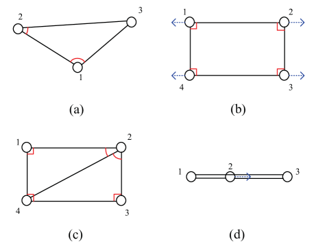
Figure 1: (a) A globally and infinitesimally angle rigid framework with $\mathcal{T}_{\mathcal{G}}^{*}=\{(1,2,3),(2,1,3)\}$. (b) A framework that is not angle rigid. (c) A globally and infinitesimally angle rigid framework with $\mathcal{T}_{\mathcal{G}}^{*}=\{(1,2,4),(2,1,4),(2,3,4),(3,2,4),(4,1,3)\}$. (d) A globally angle rigid framework with $\mathcal{T}_{\mathcal{G}}=\{(1,2,3),(2,1,3),(2,1,3)\}$.

For a framework $(\mathcal{G},p)$, the angle rigidity function corresponding to a given angle index set $\mathcal{T}_{\mathcal{G}}^{*}$ can be written as

$$f_{\mathcal{T}_{\mathcal{G}}^{*}}(p)=(\cdots,g_{ij}^{T}(p)g_{ik}(p),\cdots)^{T},~{}~{}(i,j,k)\in\mathcal{T}_{\mathcal{G}}^{*}.$$ (4)

For the sake of notational simplicity, we denote $f_{\mathcal{G}}(p)=f_{\mathcal{T}_{\mathcal{G}}}(p)$.

It is easy to see that whether $f_{\mathcal{T}_{\mathcal{G}}^{*}}(p)$ can determine a unique shape congruent to $p$ is determined by the choice of $\mathcal{T}_{\mathcal{G}}^{*}$. As a result, the definitions of angle rigidity must be associated with $\mathcal{T}_{\mathcal{G}}^{*}$. We present the following definitions.

Definition 3.

A framework $(\mathcal{G},p)$ is angle rigid if there exist an angle index set $\mathcal{T}_{\mathcal{G}}^{*}$ and a neighborhood $U_{p}$ of $p$ such that $f_{\mathcal{T}_{\mathcal{G}}^{*}}^{-1}(f_{\mathcal{T}_{\mathcal{G}}^{*}}(p))\cap U_{p}=~{}f_{\mathcal{K}}^{-1}(f_{\mathcal{K}}(p))\cap U_{p}$.

Definition 4.

A framework $(\mathcal{G},p)$ is globally angle rigid if there exists an angle index set $\mathcal{T}_{\mathcal{G}}^{*}$ such that $f_{\mathcal{T}_{\mathcal{G}}^{*}}^{-1}(f_{\mathcal{T}_{\mathcal{G}}^{*}}(p))=f_{\mathcal{K}}^{-1}(f_{\mathcal{K}}(p))$.

Definition 5.

A framework $(\mathcal{G},p)$ is minimally angle rigid if $(\mathcal{G},p)$ is angle rigid, and deletion of any edge will make $(\mathcal{G},p)$ not angle rigid.

By these definitions, the frameworks (a) and (c) in Fig. 1 are both globally angle rigid. For the framework (b), by moving the vertices along the blue arrows, $f_{\mathcal{G}}$ is invariant but the shape is deformed, thus (b) is not angle rigid. For the framework (d), since the graph is complete, it obviously holds $f_{\mathcal{G}}^{-1}(f_{\mathcal{G}}(p))=f_{\mathcal{K}}^{-1}(f_{\mathcal{K}}(p))$, thus (d) is globally angle rigid. Note that the shape of (d) still cannot be determined by angles uniquely.

Similar to distance and bearing rigidity theory, we define the infinitesimal angle motion as a motion preserving the invariance of $f_{\mathcal{T}_{\mathcal{G}}^{*}}(p)$. The velocity $v=\dot{p}$ corresponding to an infinitesimal motion should satisfy $\dot{f}_{\mathcal{T}_{\mathcal{G}}^{*}}(p)=0$, which is equivalent to the following equation

$$\dot{g}_{ij}^{T}g_{ik}+g_{ij}^{T}\dot{g}_{ik}=0,~{}~{}(i,j,k)\in\mathcal{T}_{\mathcal{G}}^{*}.$$ (5)

From [39], $\frac{\partial g_{ij}}{\partial e_{ij}}=\frac{1}{||e_{ij}||}P_{ij}$, where $P_{ij}\triangleq P(g_{ij})$, $P(\cdot):\mathbb{R}^{2}\rightarrow\mathbb{R}^{2\times 2}$ is a projection matrix defined as $P(x)=I_{2}-xx^{T}$, $x\in\mathbb{R}^{2}$ is a unit vector. Then we have $\dot{g}_{ij}=\frac{1}{||e_{ij}||}P_{ij}\dot{e}_{ij}$. Let $g(p)=(\cdots,g_{ij}^{T}(p),\cdots)^{T}$, where $(i,j)\in\mathcal{E}$, and $R_{g}\triangleq\frac{\partial f_{\mathcal{T}_{\mathcal{G}}^{*}}}{\partial g}$. It follows from the chain rule that

$$\dot{f}_{\mathcal{T}_{\mathcal{G}}^{*}}=\frac{\partial f_{\mathcal{T}_{\mathcal{G}}^{*}}}{\partial g}\frac{\partial g}{\partial e}\frac{\partial e}{\partial p}\dot{p}=R_{g}(p)\operatorname{diag}(\frac{P_{ij}}{||e_{ij}||})\bar{H}\dot{p}=R_{\mathcal{T}_{\mathcal{G}}^{*}}(p)\dot{p},$$

where $\bar{H}=H\otimes I_{2}$, $R_{\mathcal{T}_{\mathcal{G}}^{*}}(p)\triangleq R_{g}(p)\operatorname{diag}(\frac{P_{ij}}{||e_{ij}||})\bar{H}=R_{g}(p)R_{B}(p)\in\mathbb{R}^{w\times 2n}$ is termed the angle rigidity matrix, $R_{B}=\frac{\partial g(p)}{\partial p}$ is actually the bearing rigidity matrix. Therefore, equation (5) is equivalent to $R_{\mathcal{T}_{\mathcal{G}}^{*}}(p)\dot{p}=0$.

Next we define infinitesimal angle rigidity, to do this, we should distinguish all trivial motions for an angle-constrained geometric shape. By an intuitive observation, the motions always preserving invariance of angles in the framework are translations, rotations, and scalings. Therefore, the dimension of the trivial motion space is $2+1+1=4$. Note that the trivial motion space is always a subspace of $\operatorname{null}(R_{\mathcal{T}_{\mathcal{G}}^{*}})$, implying that $\dim(\operatorname{null}(R_{\mathcal{T}_{\mathcal{G}}^{*}}))\geq 4$. We present the following definition.

Definition 6.

A framework $(\mathcal{G},p)$ is infinitesimally angle rigid if there exists an angle index set $\mathcal{T}_{\mathcal{G}}^{*}$ such that every possible motion satisfying (5) is trivial, or equivalently, $\dim(\operatorname{null}(R_{\mathcal{T}_{\mathcal{G}}^{*}}))=4$.

By this definition, the frameworks in Fig. 1 (a) and (c) are both infinitesimally angle rigid. The frameworks (b) and (d) are not infinitesimally angle rigid since they both have nontrivial infinitesimal angle motions, which are interpreted by the arrows in blue.

In this paper, we say an angle index set $\mathcal{T}_{\mathcal{G}}^{*}$ supports or is suitable for (global, minimal, infinitesimal) angle rigidity of $(\mathcal{G},p)$ if $\mathcal{T}_{\mathcal{G}}^{*}$ makes the condition in the corresponding definition valid. We say $\mathcal{T}_{\mathcal{G}}^{*}$ is minimally suitable if $\mathcal{T}_{\mathcal{G}}^{*}$ is suitable and no proper subset of $\mathcal{T}_{\mathcal{G}}^{*}$ can be suitable. It is easy to see from Definitions 3-6 that the angle rigidity property of a framework $(\mathcal{G},p)$ is completely dependent on $\mathcal{G}$ and $p$. After $(\mathcal{G},p)$ is given, whether a suitable $\mathcal{T}_{\mathcal{G}}^{*}$ exists becomes certain. However, even for an angle rigid framework, there may exist $\mathcal{T}_{\mathcal{G}}^{*}$ such that the conditions in the angle rigidity definitions are invalid. For example, if we choose $\mathcal{T}_{\mathcal{G}}^{*}=\mathcal{T}_{T}$ where $T$ is a spanning tree of $\mathcal{G}$, $\mathcal{T}_{\mathcal{G}}^{*}$ can never support angle rigidity of $(\mathcal{G},p)$. On the other hand, there may exist multiple choices of $\mathcal{T}_{\mathcal{G}}^{*}$ supporting angle rigidity of a rigid framework. In Subsection 3.2, Algorithm 1 will be given to construct a suitable angle index set.

The following lemma gives the specific form of trivial motions preserving invariance of angles.

Lemma 7.

The trivial motion space for angle rigidity in $\mathbb{R}^{2}$ is $\mathcal{S}=\mathcal{S}_{r}\cup\mathcal{S}_{s}\cup\mathcal{S}_{t}$, where $\mathcal{S}_{r}=\{(I_{n}\otimes\mathscr{R}_{o}(\frac{\pi}{2}))p\}$ is the space formed by infinitesimal rotations, $\mathcal{S}_{s}=\operatorname{span}\{p\}$ is the space formed by infinitesimal scalings, $\mathcal{S}_{t}=\operatorname{null}(\bar{H})=\{\mathbf{1}_{n}\otimes(1,0)^{T},\mathbf{1}_{n}\otimes(0,1)^{T}\}$ is the space formed by infinitesimal translations.

Proof. In [39], the authors showed that $\mathcal{S}_{s}$ and $\mathcal{S}_{t}$ are scaling and translational motion spaces, respectively, and always belong to $\operatorname{null}(R_{B}(p))$. Since $R_{\mathcal{T}_{\mathcal{G}}^{*}}(p)=R_{g}(p)R_{B}(p)$, it is straightforward that $\mathcal{S}_{s}\cup\mathcal{S}_{t}\subseteq\operatorname{null}(R_{\mathcal{T}_{\mathcal{G}}^{*}}(p))$. Next we show $\mathcal{S}_{r}\subseteq\operatorname{null}(R_{\mathcal{T}_{\mathcal{G}}^{*}}(p))$.

Let $\eta^{T}=\frac{\partial g_{ij}^{T}g_{ik}}{\partial g}$ be an arbitrary row of $R_{g}$. It suffices to show $\eta^{T}R_{B}(p)(I_{n}\otimes\mathscr{R}_{o}(\frac{\pi}{2}))p=0$. Note that $\eta=(\mathbf{0},g_{ik}^{T},\mathbf{0},g_{ij}^{T},\mathbf{0})^{T}$, which follows $\eta^{T}\operatorname{diag}(\frac{P_{ij}}{||e_{ij}||})=(\mathbf{0},g_{ik}^{T}P_{ij}/||e_{ij}||,\mathbf{0},g_{ij}^{T}P_{ik}/||e_{ik}||,\mathbf{0})$. Note also that $\bar{H}(I_{n}\otimes\mathscr{R}_{o}(\frac{\pi}{2}))p=(H\otimes I_{2})(I_{n}\otimes\mathscr{R}_{o}(\frac{\pi}{2}))p=(I_{m}\otimes\mathscr{R}_{o}(\frac{\pi}{2}))(H\otimes I_{2})p=(I_{m}\otimes\mathscr{R}_{o}(\frac{\pi}{2}))e$, where $e=(\cdots,e_{ij}^{T},\cdots)^{T}$, the order of $e_{ij}$ in the vector $e$ is the same as the one of $g_{ij}$ in the vector $g$. It follows that

$$\begin{split}\eta^{T}R_{B}&(p)(I_{n}\otimes\mathscr{R}_{o}(\frac{\pi}{2}))p\\ &=\eta^{T}\operatorname{diag}(\frac{P_{ij}}{||e_{ij}||})\bar{H}(I_{n}\otimes\mathscr{R}_{o}(\frac{\pi}{2}))p\\ &=g_{ik}^{T}\frac{P_{ij}}{||e_{ij}||}\mathscr{R}_{o}(\frac{\pi}{2})e_{ij}+g_{ij}^{T}\frac{P_{ik}}{||e_{ik}||}\mathscr{R}_{o}(\frac{\pi}{2})e_{ik}\\ &=g_{ik}^{T}(I-g_{ij}g_{ij}^{T})\mathscr{R}_{o}(\frac{\pi}{2})g_{ij}+g_{ij}^{T}(I-g_{ik}g_{ik}^{T})\mathscr{R}_{o}(\frac{\pi}{2})g_{ik}\\ \end{split}$$

$$\begin{split}&=g_{ik}^{T}\mathscr{R}_{o}(\frac{\pi}{2})g_{ij}+g_{ij}^{T}\mathscr{R}_{o}(\frac{\pi}{2})g_{ik}\\ &=g_{ik}^{T}(\mathscr{R}_{o}(\frac{\pi}{2})+\mathscr{R}^{T}_{o}(\frac{\pi}{2}))g_{ij}=0.\end{split}$$

This completes the proof. $\square$

Lemma 8.

A framework $(\mathcal{G},p)$ is infinitesimally angle rigid if and only if $\operatorname{null}(R_{\mathcal{T}_{\mathcal{G}}}(p))=\mathcal{S}$.

In [3], the authors showed that the set $D_{\mathcal{K}}^{-1}(D_{\mathcal{K}}(p))$, which includes all configurations having inter-distance congruent to $p$, is always a manifold of dimension 3. In fact, since an angle-constrained shape has at least 4 degrees of freedom, $f_{\mathcal{K}}^{-1}(f_{\mathcal{K}}(p))$ is a manifold of dimension 4 when $(\mathcal{K},p)$ is infinitesimally angle rigid (i.e., $p$ is a regular point). See the following theorem.

Theorem 9.

Let $\mathscr{S}_{p}\triangleq\{q\in\mathbb{R}^{2n}:q=c(I_{n}\otimes\mathscr{R})p+\mathbf{1}_{n}\otimes\xi,\mathscr{R}\in\textrm{O(2)},c\in\mathbb{R}\setminus\{0\},\xi\in\mathbb{R}^{2}\}$. If $(\mathcal{K},p)$ is infinitesimally angle rigid, then $f_{\mathcal{K}}^{-1}(f_{\mathcal{K}}(p))=\mathscr{S}_{p}$, and $\mathscr{S}_{p}$ is a 4-dimensional manifold.

The proof will be presented in later subsections.

With the aid of Theorem 9, we can derive the relationship between infinitesimal angle rigidity and angle rigidity, which is as follows.

Theorem 10.

If $(\mathcal{G},p)$ is infinitesimally angle rigid for $\mathcal{T}_{\mathcal{G}}^{*}$, then $(\mathcal{G},p)$ is angle rigid for $\mathcal{T}_{\mathcal{G}}^{*}$.

Proof. By [3, Proposition 2] and $\operatorname{rank}\frac{\partial f_{\mathcal{T}_{\mathcal{G}}^{*}}}{\partial p}=2n-4$, there is a neighborhood $U$ of $p$, such that $f_{\mathcal{T}_{\mathcal{G}}^{*}}^{-1}(f_{\mathcal{T}_{\mathcal{G}}^{*}}(p))\cap U$ is a manifold of dimension $4$. From Theorem 9, $f_{\mathcal{K}}^{-1}(f_{\mathcal{K}}(p))$ is also a 4-dimensional manifold. As a result, $f_{\mathcal{T}_{\mathcal{G}}^{*}}^{-1}(f_{\mathcal{T}_{\mathcal{G}}^{*}}(p))$ and $f_{\mathcal{K}}^{-1}(f_{\mathcal{K}}(p))$ coincide in $U$, implying that $(\mathcal{G},p)$ is angle rigid. $\square$

The converse of Theorem 10 is not true. A typical counter-example is the framework $(\mathcal{K},p)$ with $p$ being a degenerate configuration. In this case, $(\mathcal{K},p)$ is globally angle rigid but not infinitesimally angle rigid.

3.1 The relation to infinitesimal bearing rigidity

In this subsection, we will establish some connections between angle rigidity and bearing rigidity [39, 38]. The following theorem shows the equivalence of infinitesimal angle rigidity and infinitesimal bearing rigidity in the plane, which also implies the feasibility of angle-based approach for determining a framework in the plane.

Theorem 11.

A framework $(\mathcal{G},p)$ is infinitesimally angle rigid if and only if it is infinitesimally bearing rigid.

Proof. See Appendix. A in Section 7. $\square$

Remark 12.

In [38], the authors proved that infinitesimal bearing rigidity is a generic property of the graph. That is, if $(\mathcal{G},p)$ is infinitesimally bearing rigid, then $(\mathcal{G},q)$ is infinitesimally bearing rigid for almost all configuration $q$. The underlying approach is showing that a framework embedded by a graph is either infinitesimally bearing rigid or not infinitesimally bearing rigid for all generic configurations. From Theorem 11, infinitesimal angle rigidity is also a generic property of the graph, thus is primarily determined by the graph, rather than the configuration. In fact, angle rigidity is also a generic property of the graph. To show this, it suffices to show that an angle rigid framework $(\mathcal{G},p^{*})$ with a generic configuration $p^{*}$ is always infinitesimally angle rigid. In [14, Theorem 3.17], we have shown that a generic configuration $p^{*}$ must be a regular point, i.e., $\operatorname{rank}(R_{\mathcal{T}_{\mathcal{G}}}(p^{*}))=\max_{p\in\mathbb{R}^{2n}}\operatorname{rank}(R_{\mathcal{T}_{\mathcal{G}}}(p))\triangleq\kappa$. By [3, Proposition 2], there exists a neighborhood $U$ of $p^{*}$, such that $f_{\mathcal{G}}^{-1}(f_{\mathcal{G}}(p^{*}))\cap U$ is a manifold of dimension $2n-\kappa$. From the definition of angle rigidity and Theorem 9, we know that there exists a neighborhood $U^{\prime}$ of $p^{*}$, such that $f_{\mathcal{G}}^{-1}(f_{\mathcal{G}}(p^{*}))\cap U^{\prime}$ is a manifold of dimension $4$. By definition of the manifold, we have $2n-\kappa=4$. Then $\kappa=2n-4$. That is, $(\mathcal{G},p^{*})$ is infinitesimally angle rigid. Hence, angle rigidity is also a generic property of the graph. By a similar approach, it can be easily obtained that global angle rigidity is also a generic property of the graph.

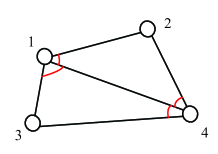
(a) $(\mathcal{G},p)$

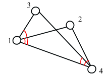
(b) $(\mathcal{G},q)$

Figure 2: Both $(\mathcal{G},p)$ and $(\mathcal{G},q)$ are infinitesimally angle rigid for $\mathcal{T}_{\mathcal{G}}^{*}=$ $\{(1,2,4),(4,1,2),(1,3,4),(4,1,3)\}$, globally angle rigid for $\bar{\mathcal{T}}_{\mathcal{G}}^{*}=\{(1,2,3)\}\cup\mathcal{T}_{\mathcal{G}}^{*}$.

Remark 13.

From Definition 6, we can conclude that the minimal number of angle constraints for achieving infinitesimal angle rigidity is $2n-4$. This fact has also been shown in [11]. On the other hand, it has been shown in [39] that the minimal number of edges for a framework to be infinitesimally bearing rigid is $2n-3$. By Theorem 11, the same is true for infinitesimal angle rigidity.

Consider a framework $(\mathcal{G},p)$ in the plane. For distance rigidity theory, it is obvious that the shape of $(\mathcal{G},p)$ can be uniquely determined by $D_{\mathcal{G}}(p)$ if $\mathcal{G}=\mathcal{K}$. For bearing rigidity theory, the authors of [39] showed that $B_{\mathcal{G}}(p)$ uniquely determines a shape if $(\mathcal{G},p)$ is infinitesimally bearing rigid. However, for angle rigidity theory, it cannot be immediately answered that whether the shape can be uniquely determined by angles between edges. This is because angles are only constraints on relationships between those edges joining a common vertex. Even for a complete graph, if $n>3$, there always exist disjoint edges, the angle between each pair of disjoint edges cannot be constrained directly.

In the following theorem, the connection between $f_{\mathcal{K}}^{-1}(f_{\mathcal{K}}(p))$ and $B_{\mathcal{K}}^{-1}(B_{\mathcal{K}}(p))$ is established.

Theorem 14.

Given configurations $p,q\in\mathbb{R}^{2n}$, $q\in f_{\mathcal{K}}^{-1}(f_{\mathcal{K}}(p))$ if and only if $(I_{n}\otimes\mathscr{R})^{-1}q\in B_{\mathcal{K}}^{-1}(B_{\mathcal{K}}(p))$, where $\mathscr{R}\in\textrm{O(2)}$.

Proof. See Appendix. B in Section 8. $\square$

(a) $(\mathcal{G},p)$

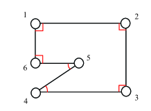
(b) $(\mathcal{G},q)$

Figure 3: $f_{\mathcal{G}}(p)=f_{\mathcal{G}}(q)$, but there does not exist $\mathscr{R}\in\textrm{O(2)}$ such that $B_{\mathcal{G}}(p)=(I_{m}\otimes\mathscr{R})B_{\mathcal{G}}(q)$. The angles in red are all constrained angles determined by $\mathcal{T}_{\mathcal{G}}$.

Remark 15.

One can realize that the validity of Theorem 14 will not be lost provided the complete graph $\mathcal{K}$ is replaced with $\mathcal{G}$, where $(\mathcal{G},p)$ is both globally angle rigid and globally bearing rigid. Note that once $\mathcal{K}$ is replaced with a general graph $\mathcal{G}$, Theorem 14 may become invalid. As shown in Fig. 3, although $q\in f_{\mathcal{G}}^{-1}(f_{\mathcal{G}}(p))$, there does not exist $\mathscr{R}\in\textrm{O(2)}$ such that $q\in(I_{n}\otimes\mathscr{R})^{-1}q\in B_{\mathcal{G}}^{-1}(B_{\mathcal{G}}(p))$.

It is important to note that Theorem 14 cannot induce equivalence of global angle rigidity and global bearing rigidity. Some examples show that this equivalence holds, but we still have no idea of how to prove it. Nonetheless, we are able to establish the following result.

Theorem 16.

If a framework $(\mathcal{G},p)$ is (globally) angle rigid, then it is (globally) bearing rigid.

Proof. Suppose $(\mathcal{G},p)$ is angle rigid. Then there exists a neighborhood $U_{p}$ of $p$ such that $f_{\mathcal{G}}^{-1}(f_{\mathcal{G}}(p))\cap U_{p}=f_{\mathcal{K}}^{-1}(f_{\mathcal{K}}(p))\cap U_{p}$. For this $U_{p}$, consider any $q\in B_{\mathcal{G}}^{-1}(B_{\mathcal{G}}(p))\cap U_{p}$. It follows from $B_{\mathcal{G}}(p)=B_{\mathcal{G}}(q)$ that $f_{\mathcal{G}}(p)=f_{\mathcal{G}}(q)$. Therefore, $f_{\mathcal{K}}(p)=f_{\mathcal{K}}(q)$. By Theorem 14, $B_{\mathcal{K}}(p)=(I_{m}\otimes\mathscr{R})B_{\mathcal{K}}(q)$ for some $\mathscr{R}\in\textrm{O(2)}$. Recall that $B_{\mathcal{G}}(p)=B_{\mathcal{G}}(q)$, we have $\mathscr{R}=I_{2}$. As a result, $B_{\mathcal{K}}(p)=B_{\mathcal{K}}(q)$, i.e., $q\in B_{\mathcal{K}}^{-1}(B_{\mathcal{K}}(p))$. That is, $(\mathcal{G},p)$ is bearing rigid.

From [39], bearing rigidity is equivalent to global bearing rigidity. Since global angle rigidity obviously leads to angle rigidity, it can also induce global bearing rigidity. $\square$

To prove Theorem 9, we introduce the following theorem in [17].

Theorem 17.

([17] Constant-Rank Level Set Theorem) Let $M$ and $N$ be smooth manifolds, and let $\Phi:M\rightarrow N$ be a smooth map, the Jacobian matrix of $\Phi$ has constant rank $r$. Each level set of $\Phi$ is a properly embedded submanifold of codimension $r$ in $M$.

Proof of Theorem 9. From Theorem 11, $(\mathcal{K},p)$ is infinitesimally bearing rigid. [39] shows that $B_{\mathcal{K}}^{-1}(B_{\mathcal{K}}(p))=\{q\in\mathbb{R}^{2n}:q=cp+\mathbf{1}_{n}\otimes\xi,c\in\mathbb{R}\setminus\{0\},\xi\in\mathbb{R}^{2}\}$. Together with Theorem 14, there must hold $f_{\mathcal{K}}^{-1}(f_{\mathcal{K}}(p))=\mathscr{S}_{p}$.

Next we show $\mathscr{S}_{p}$ is a manifold. For any $q\in f_{\mathcal{K}}^{-1}(f_{\mathcal{K}}(p))$, it is obvious that $q=(I_{n}\otimes\mathscr{R})(cp+\mathbf{1}_{n}\otimes\xi)$ for some $\mathscr{R}\in\textrm{O(2)}$, scalar $c$ and vector $\xi\in\mathbb{R}^{2}$. From the chain rule, we have

$$\begin{split}\operatorname{rank}\frac{\partial f_{\mathcal{K}}(q)}{\partial q}&=\operatorname{rank}\frac{\partial f_{\mathcal{K}}(p)}{\partial c(I_{n}\otimes\mathscr{R})p}\\ &=\operatorname{rank}\big{[}\frac{\partial f_{\mathcal{K}}(p)}{\partial p}\frac{1}{c}(I_{n}\otimes\mathscr{R}^{-1})\big{]}\\ &=2n-4.\end{split}$$

Note that $f_{\mathcal{K}}:\mathbb{R}^{2n}\rightarrow\mathbb{R}^{|\mathcal{T}_{\mathcal{K}}|}$ is a smooth map, according to Theorem 17, $f_{\mathcal{K}}^{-1}(f_{\mathcal{K}}(p))$ is a properly embedded submanifold of dimension $2n-(2n-4)=4$. $\square$

3.2 Construction of $\mathcal{T}_{\mathcal{G}}^{*}$ for infinitesimal angle rigidity

From Definition 6 it is easy to see that $\mathcal{T}_{\mathcal{G}}$ is always sufficient to determine whether a framework is infinitesimally angle rigid or not. However, the set of angles determined by $\mathcal{T}_{\mathcal{G}}$ is usually redundant. To reduce computational cost, we give an algorithm to construct a subset $\mathcal{T}_{\mathcal{G}}^{*}\subset\mathcal{T}_{\mathcal{G}}$, which is also sufficient to determine infinitesimal angle rigidity. In the proof for sufficiency of Theorem 11, we have presented an approach for constructing a set $\mathcal{T}_{\mathcal{G}}^{*}$, and proved that $\mathcal{T}_{\mathcal{G}}^{*}$ is a suitable angle index set. Here we give the following algorithm to implement this procedure.

Algorithm 1 Finding a Suitable Angle Index Set $\mathcal{T}_{\mathcal{G}}^{*}$ for Infinitesimal Angle Rigidity

1:An infinitesimally angle rigid framework $(\mathcal{G},p)$ with $p=(p_{1}^{T},\cdots,p_{n}^{T})^{T}\in\mathbb{R}^{2n}$.

2:$\mathcal{T}_{\mathcal{G}}^{*}$

3:Initialize $\mathcal{T}_{\mathcal{G}}^{*}\leftarrow\varnothing$

4:for all $i\in\mathcal{V}$ do

5:     Initialize ${}^{i}\mathcal{T}_{\mathcal{G}}^{*}\leftarrow\varnothing$

6:     Compute the neighbor set of $i$ in $\mathcal{G}$, i.e., $\mathcal{N}_{i}$

7:     Select $j_{i}$ from $\mathcal{N}_{i}$ randomly, $\hat{\mathcal{N}}_{i}\leftarrow\{j_{i}\}\cup\{k\in\mathcal{N}_{i}:p_{i}-p_{j_{i}}~{}is~{}collinear~{}with~{}p_{i}-p_{k}\}$, $\check{\mathcal{N}}_{i}\leftarrow\mathcal{N}_{i}\setminus\hat{\mathcal{N}}_{i}$

8:     ${}^{i}\mathcal{T}_{\mathcal{G}}^{*}\leftarrow~{}^{i}\mathcal{T}_{\mathcal{G}}^{*}\cup(i,j_{i},k)$ for all $k\in\check{\mathcal{N}}_{i}$. Proceed only if $|\hat{\mathcal{N}}_{i}|>1$

9:     Select $k_{i}$ from $\check{\mathcal{N}}_{i}$ randomly

10:     for all $j\in\hat{\mathcal{N}}_{i}\setminus\{j_{i}\}$ do

11:         ${}^{i}\mathcal{T}_{\mathcal{G}}^{*}\leftarrow~{}^{i}\mathcal{T}_{\mathcal{G}}^{*}\cup(i,j,k_{i})$ if $j<k_{i}$, ${}^{i}\mathcal{T}_{\mathcal{G}}^{*}\leftarrow~{}^{i}\mathcal{T}_{\mathcal{G}}^{*}\cup(i,k_{i},j)$ otherwise

12:     end for

13:     $\mathcal{T}_{\mathcal{G}}^{*}\leftarrow~{}^{i}\mathcal{T}_{\mathcal{G}}^{*}$

14:end for

15:return $\mathcal{T}_{\mathcal{G}}^{*}$

Since each vertex has at most $n-1$ neighbors, it is easy to see that the number of elementary operations performed by Algorithm 1 is at most $n(n-2)$. Hence the time complexity of Algorithm 1 is $\mathcal{O}(n^{2})$.

An example of constructing ${}^{i}\mathcal{T}_{\mathcal{G}}^{*}$ by Algorithm 1 is shown in Fig. 4.

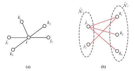
Figure 4: An example to illustrate the construction of ${}^{i}\mathcal{T}_{\mathcal{G}}^{*}$ by Algorithm 1. (a) The subgraph composed of vertex $i$ and its neighbors $j_{1}$, $j_{2}$, $k_{1}$, $k_{2}$, $k_{3}$. Note that $i,k_{2},k_{3}$ are collinear, $i,j_{1},j_{2}$ are collinear. (b) $\hat{\mathcal{N}}_{i}=\{j_{1},j_{2}\}$, $\check{\mathcal{N}}_{i}=\{k_{1},k_{2},k_{3}\}$. If $j_{s}$ and $k_{l}$ are connected by a red line, it implies that the angle between edge $(i,j_{s})$ and edge $(i,k_{l})$ is selected to be constrained. This also implies that $(i,j_{s},k_{l})$ (if $j_{s}<k_{l}$) or $(i,k_{l},j_{s})$ (if $k_{l}<j_{s}$) is an element of ${}^{i}\mathcal{T}_{\mathcal{G}}^{*}$.

Note that for an infinitesimally angle rigid framework, the angle index set generated by Algorithm 1 is suitable but not minimally suitable for infinitesimal angle rigidity. For example, let $(\mathcal{G},p)$ be a minimally angle rigid framework, then $|\mathcal{E}|=2n-3$. For a set $\mathcal{T}_{\mathcal{G}}^{*}$ generated by Algorithm 1, we have $|\mathcal{T}_{\mathcal{G}}^{*}|=\sum_{i\in\mathcal{V}}|^{i}\mathcal{T}_{\mathcal{G}}^{*}|=\sum_{i\in\mathcal{V}}(|\mathcal{N}_{i}|-1)=2(2n-3)-n=3n-6\geq 2n-4$ for $n\geq 2$. Currently we do not have an algorithm to construct a minimally suitable angle index set for an arbitrary infinitesimally angle rigid framework.

Remark 18.

Although $\mathcal{T}_{\mathcal{G}}^{*}$ constructed by Algorithm 1 supports infinitesimal angle rigidity, it may not support global angle rigidity. As shown in Fig. 2 (a), by Algorithm 1, we can obtain $\mathcal{T}_{\mathcal{G}}^{*}=\{(1,2,4),(4,1,2),(1,3,4),(4,1,3)\}$. Although $(\mathcal{G},p)$ is infinitesimally angle rigid, $f_{\mathcal{T}_{\mathcal{G}}^{*}}(p)$ may determine an incorrect shape as shown in Fig. 2 (b). However, if we let $\bar{\mathcal{T}}_{\mathcal{G}}^{*}=\{(1,2,3)\}\cup\mathcal{T}_{\mathcal{G}}^{*}$, then $f_{\bar{\mathcal{T}}_{\mathcal{G}}^{*}}(p)$ can always determine a correct shape. This implies that $(\mathcal{G},p)$ in Fig 2 (a) is both infinitesimally and globally angle rigid for $\bar{\mathcal{T}}_{\mathcal{G}}^{*}(p)$.

In fact, even for a complete graph, it is possible that the geometric shape cannot be determined by angle-only or bearing-only information. A typical example is the degenerate configuration shown in Fig. 1 (d). Generally, we hope to determine a framework $(\mathcal{G},p)$ by angles uniquely up to translations, rotations, scalings and reflections in the plane. That is, $f_{\mathcal{G}}^{-1}(f_{\mathcal{G}}(p))=\mathscr{S}_{p}$. In the next subsection, we will introduce a specific class of frameworks satisfying this condition.

3.3 A class of frameworks uniquely determined by angles

In [7], the authors introduced a particular class of Laman graphs termed triangulated Laman graphs, which are constructed by a modified Henneberg insertion procedure. In what follows, we will show that the shape of such frameworks can always be determined by angles uniquely. Let $\mathcal{L}_{n}=(\mathcal{V}_{n},\mathcal{E}_{n})$ be an $n-$point($n\geq 3$) triangulated Laman graph, its definition is as follows.

Definition 19.

Let $\mathcal{L}_{2}$ be the graph with vertex set $\mathcal{V}_{2}=\{1,2\}$ and edge set $\mathcal{E}_{2}=\{(1,2)\}$. $\mathcal{L}_{n}$ ($n\geq 3$) is a graph obtained by adding a vertex $n$ and two edges $(n,i)$, $(n,j)$ into graph $\mathcal{L}_{n-1}$ for some $i$ and $j$ satisfying $(i,j)\in\mathcal{E}_{n-1}$.

Note that the triangulated Laman graph considered here is an undirected graph. Now we give the following result for frameworks embedded by triangulated Laman graphs.

Lemma 20.

A triangulated framework $(\mathcal{L}_{n},p)$ is infinitesimally distance rigid if and only if $(\mathcal{L}_{n},p)$ is strongly nondegenerate, i.e., $p_{i}$, $p_{j}$ and $p_{k}$ are not collinear for any three vertices $i,j,k$ satisfying $(i,j),(j,k),(i,k)\in\mathcal{E}_{n}$.

Proof. The proof for sufficiency has been given in [7]. Next we give the proof for necessity. Suppose that strong nondegeneracy does not hold, then there exist $i,j,k\in\mathcal{V}$, such that $(i,j),(j,k),(i,k)\in\mathcal{E}_{n}$ and $p_{i},p_{j},p_{k}$ stay collinear. Note that $(\mathcal{L}_{n},p)$ has exactly $2n-3$ edges. Let $R_{D}(p)=\frac{\partial D_{\mathcal{G}}(p)}{\partial p}\in\mathbb{R}^{(2n-3)\times 2n}$ be the distance rigidity matrix. To guarantee $\operatorname{rank}(R_{D}(p))=2n-3$, $R_{D}(p)$ should be of full row rank. However, it is easy to see that $\frac{\partial||e_{ij}||^{2}}{\partial p}$, $\frac{\partial||e_{ik}||^{2}}{\partial p}$, and $\frac{\partial||e_{jk}||^{2}}{\partial p}$ are always linearly dependent. Hence, $R_{D}(p)$ cannot be of full row rank, which is a contradiction. $\square$

The following theorem shows that the shape of a strongly nondegenerate triangulated framework in the plane can always be uniquely determined by angles.

Theorem 21.

A triangulated framework $(\mathcal{L}_{n},p)$ is strongly nondegenerate

(i) if and only if $(\mathcal{L}_{n},p)$ is minimally infinitesimally angle rigid. A minimally suitable angle index set is

$$\mathcal{T}_{\mathcal{L}_{n}}^{*}=\{(i,j,k)\in\mathcal{V}^{3}_{n}:~{}~{}(i,j),(j,k),(i,k)\in\mathcal{E}_{n},~{}i,j<k\};$$ (6)

(ii) only if $(\mathcal{L}_{n},p)$ is globally angle rigid. A minimally suitable angle index set is $\mathcal{T}_{\mathcal{L}_{n}}^{\dagger}=\mathcal{T}_{\mathcal{L}_{n}}^{*}\cup\Delta\mathcal{T}_{\mathcal{L}_{n}}$, where $\Delta\mathcal{T}_{\mathcal{L}_{n}}=\{(i,k,l):k=\min\{\mathcal{N}_{i}\cap\mathcal{N}_{j}\cap\mathcal{V}_{l-1}\},i,j\in\mathcal{N}_{l},~{}i<j<l,l=4,\cdots,n\}$ if $n\geq 4$, and $\Delta\mathcal{T}_{\mathcal{L}_{n}}=\varnothing$ otherwise.

Proof. See Appendix. C in Section 9. $\square$

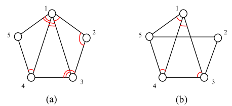
Figure 5: (a) A framework embedded by a triangulated Laman graph $\mathcal{L}_{5}$. $(\mathcal{L}_{5},p)$ is infinitesimally angle rigid for $\mathcal{T}_{\mathcal{L}_{5}}^{*}=\{(1,2,3),(1,3,4),(1,4,5),(2,1,3),(3,1,4),$ $(4,1,5)\}$, and globally angle rigid for $\mathcal{T}_{\mathcal{L}_{5}}^{\dagger}=\mathcal{T}_{\mathcal{L}_{5}}^{*}\cup\{(1,2,4),(1,3,5)\}$. The angles in red are constrained angles determined by $\mathcal{T}_{\mathcal{L}_{5}}^{\dagger}$. (b) A framework embedded by a Laman graph that is not triangulated. The framework is globally and infinitesimally angle rigid, but $\mathcal{T}_{\mathcal{L}_{n}}^{*}$ is not sufficient for its global and infinitesimal angle rigidity. The angles in red are constrained angles determined by $\mathcal{T}_{\mathcal{L}_{n}}^{*}$.

An example of strongly nondegenerate framework embedded by a triangulated Laman graph is shown in Fig. 5 (a). The angles in red are constrained angles determined by $\mathcal{T}_{\mathcal{L}_{5}}^{\dagger}$. The framework in Fig. 5 (b) is both globally angle rigid and infinitesimally angle rigid, but it is not embedded by a triangulated Laman graph.

It is important to note that strong nondegeneracy is not necessary for a triangulated framework to be globally angle rigid. A simple counterexample is the framework shown in Fig. 1 (d). The framework is globally angle rigid, but not strongly nondegenerate. Moreover, the angle index set we give in Theorem 21 is only one suitable choice, there are also other choices of the angle index set supporting minimal infinitesimal angle rigidity or global angle rigidity of $(\mathcal{L}_{n},p)$.

4 Application to formation control

In this section, we apply angle rigidity theory to distributed formation control in the plane. The target formation will be characterized by some constraints on angles. In order to form a desired shape, the group of agents are required to meet these constraints via a distributed controller.

4.1 The formation stabilization problem

Consider $n$ agents moving in the plane, each agent $i$ has a simple kinematic point dynamics

$$\dot{p}_{i}=u_{i},~{}~{}~{}i\in\mathcal{V},$$ (7)

where $p_{i}\in\mathbb{R}^{2}$ and $u_{i}\in\mathbb{R}^{2}$ are the position and control input of agent $i$, respectively, in the global coordinate frame. We consider that the global coordinate system is absent for the agents, each agent $i$ has its own local coordinate system. Let $p^{i}_{j}$ be the coordinate of agent $j$’s position with respect to agent $i$’s local coordinate system. Agent $i$ can measure the relative position state $p^{i}_{i}-p^{i}_{k}$ if $k\in\mathcal{N}_{i}$.

In this paper, we employ an infinitesimally angle rigid framework $(\mathcal{G},p^{*})$ to describe the target formation shape. Each agent is viewed as a vertex of the framework. An interaction link between two agents is regarded as an edge in graph $\mathcal{G}$. That is, $\mathcal{G}$ is also the sensing graph interpreting the interaction relationship between agents.

The target formation shape can be defined as the following manifold:

$$\mathscr{E}=~{}\mathscr{S}_{p^{*}}=\{p\in\mathbb{R}^{2n}:p=c(I_{n}\otimes\mathscr{R})p^{*}+\mathbf{1}_{n}\otimes\xi,\\ \mathscr{R}\in\textrm{O(2)},c\in\mathbb{R}\setminus\{0\},\xi\in\mathbb{R}^{2}\}.$$

For the target formation $(\mathcal{G},p^{*})$, we make the following assumption:

Assumption 22.

Graph $\mathcal{G}$ contains a triangulated Laman graph $\mathcal{L}_{n}$ as a subgraph, and $(\mathcal{L}_{n},p^{*})$ is strongly nondegenerate.

The set determining all angle constraints is given by

$$\mathcal{T}_{\mathcal{G}}^{F}=\{(i,j,k)\in\mathcal{V}^{3}:(i,j),(j,k),(i,k)\in\mathcal{E},~{}i,j<k\},$$ (8)

Remark 23.

Assumption 22 is a graphical condition for $(\mathcal{G},p^{*})$, and will be the only condition for achieving stability of the target formation. Once Assumption 22 holds, it is easy to see that $\mathcal{T}^{*}_{\mathcal{L}_{n}}\subset\mathcal{T}_{\mathcal{G}}^{F}$, where $\mathcal{T}^{*}_{\mathcal{L}_{n}}$ is in form (6). Since we have shown in Theorem 21 that $(\mathcal{L}_{n},p^{*})$ is infinitesimally angle rigid for $\mathcal{T}^{*}_{\mathcal{L}_{n}}$, together with $\mathcal{E}_{n}\subset\mathcal{E}$, it follows that $(\mathcal{G},p^{*})$ is infinitesimally angle rigid for $\mathcal{T}_{\mathcal{G}}^{F}$. It is also worth noting that strongly nondegenerate configurations form a dense subset of $\mathbb{R}^{2n}$, which is shown in [7].

Problem 24.

Given a set of angle constraints $\mathcal{C}=\{g_{ij}^{T}(p)g_{ik}(p)=g_{ij}^{T}(p^{*})g_{ik}(p^{*})\}$ generated by a framework $(\mathcal{G},p^{*})$ satisfying Assumption 22, design a distributed control law for each agent $i$ based on the relative position measurements $\{p^{i}_{i}-p^{i}_{j},~{}j\in\mathcal{N}_{i}\}$, such that $\mathscr{E}$ is asymptotically stable.

4.2 A steepest descent formation controller

According to the set $\mathcal{C}$, we define the following set as our target equilibrium set of the formation system

$$\mathscr{E}_{F}=\{p\in\mathbb{R}^{2n}:g_{ij}^{T}(p)g_{ik}(p)=g_{ij}^{T}(p^{*})g_{ik}(p^{*}),\\ (i,j,k)\in\mathcal{T}_{\mathcal{G}}^{F}\}.$$ (9)

Note that $\mathscr{E}$ is a subset of $\mathscr{E}_{F}$. $\mathscr{E}=\mathscr{E}_{F}$ if and only if $(\mathcal{G},p^{*})$ is globally angle rigid for $\mathcal{T}_{\mathcal{G}}^{F}$. In Fig. 5 (a), the framework is only infinitesimally angle rigid, even if all the angle constraints determined by $\mathcal{T}_{\mathcal{G}}^{F}$ are satisfied, it is possible that the target formation shape is not formed. Nevertheless, from the definition of angle rigidity, for any $q\in\mathscr{E}$, there exists a neighborhood $U$ of $q$, such that $\mathscr{E}\cap U=\mathscr{E}_{F}\cap U$. Hence, stability of $\mathscr{E}_{F}$ can still be sufficient for local stability of $\mathscr{E}$.

Denote $g_{ij}=g_{ij}(p)$, $g_{ij}^{*}=g_{ij}(p^{*})$ for all $(i,j)\in\mathcal{E}$, $\delta_{(i,j,k)}=g_{ij}^{T}g_{ik}-g_{ij}^{*T}g_{ik}^{*}$, $(i,j,k)\in\mathcal{T}_{\mathcal{G}}^{*}$. To ensure convergence of (9), the multi-agent system should minimize the following cost function:

$$V_{F}(p)=\frac{1}{2}\sum_{(i,j,k)\in\mathcal{T}_{\mathcal{G}}^{*}}(g_{ij}^{T}g_{ik}-g_{ij}^{*T}g_{ik}^{*})^{2}=\frac{1}{2}\sum_{(i,j,k)\in\mathcal{T}_{\mathcal{G}}^{*}}\delta_{(i,j,k)}^{2}.$$ (10)

On the basis of function (10), a gradient-based control strategy can be derived as

$$\begin{split}u_{i}^{F}&=-\nabla_{p_{i}}V_{F}(p)\\ &=-\sum_{(j,k)\in\mathcal{N}_{\mathcal{T}_{i}}}y_{1}(e_{ij},e_{ik})-\sum_{(j,k)\in\mathcal{N}_{\mathcal{T}^{i}}}y_{2}(e_{ji},e_{jk}),i\in\mathcal{V}\end{split}$$ (11)

where $\mathcal{N}_{\mathcal{T}_{i}}=\{(j,k)\in\mathcal{V}^{2}:(i,j,k)\in\mathcal{T}_{\mathcal{G}}^{F}\}$, $\mathcal{N}_{\mathcal{T}^{i}}=\{(j,k)\in\mathcal{V}^{2}:(j,i,k)~{}or~{}(j,k,i)\in\mathcal{T}_{\mathcal{G}}^{F}\}$, $y_{1}(e_{ij},e_{ik})=(g_{ij}^{T}g_{ik}-g_{ij}^{*T}g_{ik}^{*})(\frac{P_{ij}}{||e_{ij}||}g_{ik}+\frac{P_{ik}}{||e_{ik}||}g_{ij})$, $y_{2}(e_{ji},e_{jk})=(g_{ji}^{T}g_{jk}-g_{ji}^{*T}g_{jk}^{*})\frac{P_{ij}}{||e_{ij}||}g_{kj}$.

Observe that if $(j,i,k)\in\mathcal{T}_{\mathcal{G}}^{F}$, the control input of agent $i$ includes a term associated with $e_{jk}$. This can be obtained by simple subtraction $e_{ik}-e_{ij}$. From the form of $\mathcal{T}_{\mathcal{G}}^{F}$ in (8), we have $k,j\in\mathcal{N}_{i}$. Therefore, $u_{i}^{F}$ is a distributed control strategy.

Let $\delta(p)=(\cdots,\delta_{(i,j,k)},\cdots)^{T}=f_{\mathcal{T}_{\mathcal{G}}^{F}}(p)-f_{\mathcal{T}_{\mathcal{G}}^{F}}(p^{*})$, $(i,j,k)\in\mathcal{T}_{\mathcal{G}}^{*}$. By the chain rule, the multi-agent system (7) with control input (11) can be written in the following compact form

$$\dot{p}=-\nabla_{p}V_{F}(p)=-R_{\mathcal{T}_{\mathcal{G}}^{F}}^{T}(p)\delta(p).$$ (12)

The formation system (12) has the following easily checked properties.

Lemma 25.

Under the control law (11), the following statements hold:

(i) The global coordinate system is not required for each agent.

(ii) If $p(0)$ is degenerate, then $p(t)=p(0)$ for $t\geq 0$.

(iii) The centroid $p^{o}(t)=\frac{1}{n}\sum_{i\in\mathcal{V}}p_{i}(t)$ and the scale $s(t)=\sqrt{\frac{1}{n}\sum_{i\in\mathcal{V}}||p_{i}(t)-p^{o}(t)||^{2}}$ are both invariant.

Proof. The proof of (i) is straightforward by a similar approach to those of [22, 28], the validity of (ii) is also easy to verify. Thus their proofs are omitted here. For (iii), observe that $p^{o}(t)=\frac{1}{n}p^{T}(t)\mathbf{1}_{n}$, according to (12), we have

$$\dot{p}^{o}=\frac{1}{n}\dot{p}^{T}\mathbf{1}_{n}=\frac{1}{n}\delta^{T}R_{\mathcal{T}_{\mathcal{G}}^{F}}\mathbf{1}_{n}=0.$$

To show $\dot{s}=0$, we first note that $\dot{p}^{T}p=\delta^{T}R_{\mathcal{T}_{\mathcal{G}}^{F}}p=\delta^{T}R_{g}\operatorname{diag}(\frac{P_{ij}}{||e_{ij}||})\bar{H}p=0$. It follows that

$$\begin{split}\dot{s}&=\frac{2}{\sqrt{n}}\dot{p}^{T}(p-\mathbf{1}_{n}\otimes p^{o})\\ &=-\frac{2}{\sqrt{n}}\delta^{T}\operatorname{diag}(\frac{P_{ij}}{||e_{ij}||})\bar{H}(\mathbf{1}_{n}\otimes p^{o})=0.\end{split}$$

$\square$

4.3 Stability analysis

Theorem 26.

For a group of $n\geq 3$ agents with dynamics (7) and controller (11) moving in the plane. Under Assumption 22, for any $q\in\mathscr{E}$, there is a neighborhood $U_{q}$ of $q$, such that if $p(0)\in U_{q}$, then $\lim_{t\rightarrow\infty}p(t)=p^{\dagger}$ for some $p^{\dagger}\in\mathscr{E}$.

Proof. For any $q\in\mathscr{E}$, let $\rho=p-q$, $f(p)=-R_{\mathcal{T}_{\mathcal{G}}^{F}}^{T}(p)\delta(p)$, expanding $f(p)$ in Taylor series about $q$, we have $f(p)=f(q)+\frac{\partial f(q)}{\partial p}\rho+g(\rho)$. Then (12) is equivalent to

$$\dot{\rho}=\frac{\partial f(q)}{\partial p}\rho+g(\rho)=J_{f}(q)\rho+g(\rho),$$ (13)

where $J_{f}(q)=\frac{\partial f(q)}{\partial p}=-\frac{\partial R_{\mathcal{T}_{\mathcal{G}}^{F}}^{T}(q)}{\partial p}\delta(q)-R_{\mathcal{T}_{\mathcal{G}}^{F}}^{T}(q)\frac{\partial\delta(q)}{\partial p}=-R_{\mathcal{T}_{\mathcal{G}}^{F}}^{T}(q)R_{\mathcal{T}_{\mathcal{G}}^{F}}(q)$. From Lemma 20, the validity of Assumption 1 implies that $(\mathcal{G},q)$ is infinitesimally angle rigid. Therefore, $J_{f}(q)$ has 4 zero eigenvalues and the rest are negative real numbers. There must exist an orthonormal transformation $Q\in\mathbb{R}^{2n\times 2n}$ such that $QJ_{f}(q)Q^{T}=\operatorname{diag}(\mathbf{0}_{4\times 4},\tilde{J})$, where $\tilde{J}$ is Hurwitz. Then (13) is equivalent to

$$\begin{split}&\dot{\varphi}=g_{1}(\varphi,\psi),\\ &\dot{\psi}=\tilde{J}\psi+g_{2}(\varphi,\psi),\end{split}$$ (14)

where $(\varphi^{T},\psi^{T})^{T}=Q\rho$, $(g_{1}^{T},g_{2}^{T})^{T}=Qg(\rho)$. Note that $\rho=0$ is an equilibrium point of (13), hence, $g_{1}(0,0)=0$ and $g_{2}(0,0)=0$. Since $g(\rho)=f(p)-J_{f}(q)\rho$, we have $J_{g}|_{\rho=0}=0$. It follows that $J_{g_{1}}(0,0)=0$ and $J_{g_{2}}(0,0)=0$. Observe that $\mathcal{M}=\{(\varphi^{T},\psi^{T})^{T}:(\varphi^{T},\psi^{T})^{T}=Q\rho,\rho+q\in\mathscr{E}\}$ is a 4-dimensional manifold. We next show $\mathcal{M}$ is a center manifold. Note that $\mathcal{M}$ is invariant since $\mathscr{E}\subset\mathscr{E}_{F}\subset\{p\in\mathbb{R}^{2n}:f(p)=0\}$. Any equilibria must satisfy $\tilde{J}\psi+g_{2}(\varphi,\psi)=0$, by implicit function theorem, there is a neighborhood $U$ of the origin, such that $\psi=h(\varphi)$ for $\psi\in U$, where $h(\cdot):\mathbb{R}^{4}\rightarrow\mathbb{R}^{2n-4}$ is smooth and $h(0)=0$, $J_{h}(0)=0$. Since $\mathcal{M}$ is a 4-dimensional manifold, there must exist an open set in $\mathbb{R}^{4}$ that is diffeomorphic to a neighborhood $U^{\prime}$ of origin in $\mathcal{M}$. Because $\mathcal{M}$ can be represented by $(\varphi^{T},h^{T}(\varphi))^{T}$ in $U\cap U^{\prime}$, we conclude that $\mathcal{M}$ is a center manifold. The flow on the manifold $\mathcal{M}$ is governed by the 4-dimensional system $\dot{\xi}=g_{1}(\xi,h(\xi))$ for sufficiently small $\xi$. Recall that $\mathcal{M}$ is a manifold of equilibria, we have $\dot{\xi}=0$. By center manifold theory [6], for any sufficiently small $\varphi(0),\psi(0)$, we have $\varphi(t)=\xi(0)+O(e^{-\gamma t})$, $\psi=h(\xi(0))+O(e^{-\gamma t})$ for some $\gamma>0$. This implies that $\lim_{t\rightarrow\infty}(\varphi^{T},\psi^{T})^{T}=(\xi^{T}(0),h^{T}(\xi(0)))^{T}\in\mathcal{M}$. It follows that $\lim_{t\rightarrow\infty}p(t)=\lim_{t\rightarrow\infty}Q^{T}(\varphi^{T},\psi^{T})^{T}+q=Q^{T}(\xi^{T}(0),h^{T}(\xi(0)))^{T}+q=p^{\dagger}\in\mathscr{E}$. The proof is completed. $\square$

The difficulties in achieving global stability of the desired formation shape are two folds: (i). Observe that the equilibrium set of system (12) is $E=\{p\in\mathbb{R}^{2n}:R_{\mathcal{T}_{\mathcal{G}}^{F}}^{T}(p)\delta=0\}$. If $R_{\mathcal{T}_{\mathcal{G}}^{F}}\in\mathbb{R}^{|\mathcal{T}_{\mathcal{G}}^{F}|\times 2n}$ is of full row rank, then $p\in E$ implies $\delta=0$, which yields $p\in\mathscr{E}_{F}$. However, $R_{\mathcal{T}_{\mathcal{G}}^{F}}(p)$ varies as the formation system evolves, it is difficult to determine its rank. Moreover, once $|\mathcal{T}_{\mathcal{G}}^{F}|>2n-4$, $R_{\mathcal{T}_{\mathcal{G}}^{F}}$ can never be of full row rank. As a result, undesired equilibria often exist for system (12). (ii). Different from displacement, distance and bearing constraints on pairwise agents, each angle constraint involves three agents. The form of $\mathcal{T}_{\mathcal{G}}^{F}$ implies that only those angles in triangles can be used as constraints to determine the shape. Nevertheless, in some cases these constraints cannot uniquely determine the desired formation shape. For example, consider the framework in Fig. 5 (a), although its shape can be uniquely determined by angles, it cannot be uniquely determined by angles corresponding to $\mathcal{T}_{\mathcal{G}}^{F}$. Fig. 7 shows a counterexample that under some initial condition, the agents exponentially form an incorrect formation.

Theorem 26 actually means that by implementing the control law (11), the agents can cooperatively restore the desired formation shape under a small perturbation from any $q\in\mathscr{E}$, and the convergence rate is as fast as $e^{-\gamma t}$ for some $\gamma>0$ dependent on $q$. However, it is uncertain that whether there exists a uniform exponent $\gamma$ for all $q\in\mathscr{E}$. This is because $\mathscr{E}$ is not compact, there does not exist a finite subcover containing $\mathscr{E}$.

4.4 Orientation and scaling control

We have shown that the angle-constrained formation has 4 degrees of freedom, which is higher than that of displacement-, distance-, and bearing-based formations. This ensures that one advantage of the angle-based formation approach is the convenience of orientation and scaling control. In this subsection, we propose an angle-based control scheme to steer all agents to form a target formation shape with pre-specified orientation and scale.

Given $(\mathcal{G},p^{*})$ as the target formation shape satisfying Assumption 22, a configuration forming the target formation with desired orientation and scale can be written by $p=c^{*}(I_{n}\otimes\mathscr{R}_{o}(\theta^{*}))p^{*}+\mathbf{1}_{n}\otimes\xi$ for some constant $\theta^{*}\in[0,2\pi)$, $c^{*}\in\mathbb{R}\setminus\{0\}$ and an arbitrary translational vector $\xi\in\mathbb{R}^{2}$. It is worth noting that $p_{i}^{*}$ here denotes the position of agent $i$ in the global coordinate frame. Let $\tilde{p}=c^{*}(I_{n}\otimes\mathscr{R}_{o}(\theta^{*}))p^{*}$, then the target equilibrium can be described as

$$\mathscr{E}_{M}=\{p\in\mathbb{R}^{2n}:p=\tilde{p}+\mathbf{1}_{n}\otimes\xi,\xi\in\mathbb{R}^{2}\}.$$ (15)

To control the orientation of the formation, it is obviously necessary that some agents should have access to the global coordinate system. To keep the target shape in a precise orientation, we will try to constrain the displacement between two adjacent agents, which is similar to [28]. Since orientation and scale of the ultimate formation are determined by these two agents, we call them leaders. It is noteworthy that any two adjacent agents can be selected as leaders, and controlling their relative position is sufficient to control the orientation and scale of the formation (this fact will be shown later). Moreover, different from [28], using angle-based approach, the target displacement between leaders can be artificially specified and does not have to satisfy a fixed length constraint.

Suppose agents $l_{1}$ and $l_{2}$ are leaders, $l_{1},l_{2}\in\mathcal{V}$. Then $\tilde{p}_{l_{1}}-\tilde{p}_{l_{2}}$ is the displacement of $l_{1}$ and $l_{2}$ in the formation with target orientation and scale. Now we summarize the problem that we will deal with in this subsection as below.

Problem 27.

Given a realizable target formation $(\mathcal{G},p^{*})$ satisfying Assumption 22, and the target displacement $\tilde{p}_{l_{1}}-\tilde{p}_{l_{2}}$ known by agents $l_{1}$ and $l_{2}$, design a distributed control law for each agent $i$ based on the relative position measurements $\{p^{i}_{i}-p^{i}_{j},~{}j\in\mathcal{N}_{i}\}$, such that $\mathscr{E}_{M}$ is asymptotically stable.

To solve Problem 27, we consider the following set containing the target equilibrium $\mathscr{E}_{M}$

$$\mathscr{E}_{l}=\{p\in\mathscr{E}_{F}:p_{l_{1}}-p_{l_{2}}=\tilde{p}_{l_{1}}-\tilde{p}_{l_{2}}\},$$ (16)

where $\mathcal{E}_{F}$ is in the form (9).

The following lemma shows that once $(\mathcal{G},p^{*})$ is infinitesimally angle rigid, $\mathscr{E}_{l}$ and $\mathscr{E}_{M}$ coincide near each point in $\mathscr{E}_{M}$.

Lemma 28.

If $(\mathcal{G},p^{*})$ is infinitesimally angle rigid, then for any $q\in\mathscr{E}_{M}$, there exists a neighborhood $U_{q}$ of $q$, such that $\mathscr{E}_{M}\cap U_{q}=\mathscr{E}_{l}\cap U_{q}$.

Proof. Let $f_{l}(p)=\begin{pmatrix}f(p)\\ p_{l_{1}}-p_{l_{2}}\end{pmatrix}\in\mathbb{R}^{|\mathcal{T}_{\mathcal{G}}^{F}|+2}$, $f_{M}(p)=(\cdots,(p_{i}-p_{j})^{T},\cdots)^{T}\in\mathbb{R}^{2m}$, it follows that $\mathscr{E}_{l}=f_{l}^{-1}(f_{l}(\tilde{p}))$, $\mathscr{E}_{M}=f_{M}^{-1}(f_{M}(\tilde{p}))$. Since $\mathcal{G}$ must be connected, we have $\operatorname{rank}(\frac{\partial f_{M}}{\partial p})=\operatorname{rank}(\bar{H})=2n-2$, here $\bar{H}$ is the incidence matrix, according to Theorem 17, $\mathscr{E}_{M}$ is a 2-dimensional manifold.

Next we show $\mathscr{E}_{l}$ is also a 2-dimensional manifold near each $q\in\mathscr{E}_{M}$. Without loss of generality, suppose $p_{l_{1}}-p_{l_{2}}$ is consisted of the $(2k-1)$-th row and $2k$-th row of $\bar{H}p$. Let $S=[S_{ij}]\in\mathbb{R}^{2\times 2m}$ be a matrix with $S_{1,2k-1}=S_{2,2k}=1$, and $S_{ij}=0$ for other $i,j$. Then $S\bar{H}p=p_{l_{1}}-p_{l_{2}}$ and $\frac{\partial(p_{l_{1}}-p_{l_{2}})}{\partial p}=S\bar{H}$. For any $q\in\mathscr{E}_{M}$, denote $R_{l}(q)=\frac{\partial f_{l}}{\partial p}|_{p=q}=(R_{\mathcal{T}_{\mathcal{G}}^{F}}^{T}(q),(S\bar{H})^{T})^{T}$, it is easy to obtain $\operatorname{null}(R_{l}(q))=\operatorname{null}(R_{\mathcal{T}_{\mathcal{G}}^{F}}(q))\cap\operatorname{null}(S\bar{H})$. We first notice that $(\mathcal{G},q)$ must be infinitesimally angle rigid, implying $\operatorname{null}(R_{\mathcal{T}_{\mathcal{G}}^{F}}(q))=\mathcal{S}$, where $\mathcal{S}$ is the trivial motion space shown in Lemma 7. We also note that $\operatorname{null}(S\bar{H})=(\operatorname{null}(S)\cap\operatorname{range}(\bar{H}))\cup\operatorname{null}(\bar{H})$. It can be verified that $\operatorname{null}(R_{l}(q))=\mathcal{S}\cap\operatorname{null}(S\bar{H})=\operatorname{null}(\bar{H})=\operatorname{span}\{\mathbf{1}_{n}\otimes I_{2}\}$. Then we obtain $\operatorname{rank}(\frac{\partial f_{l}}{\partial p}|_{p=q})=2n-2=\max\{\operatorname{rank}(\frac{\partial f_{l}}{\partial p}):p\in\mathbb{R}^{2n}\}$, i.e., $q$ is a regular point of $f_{l}$. From [3, Proposition 2], there exists a neighborhood $U$ of $q$, such that $\mathscr{E}_{l}\cap U$ is a 2-dimensional manifold. Together with $\mathscr{E}_{M}\subset\mathscr{E}_{l}$, we have $\mathscr{E}_{M}\cap U\subset\mathscr{E}_{l}\cap U$. It follows that $\mathscr{E}_{l}\cap U_{q}=\mathscr{E}_{M}\cap U_{q}$ for some $U_{q}\subset U$. $\square$

By virtue of Lemma 28, when the initial positions of agents are close to $\mathscr{E}_{M}$, to drive the agents into $\mathscr{E}_{M}$, it suffices to constrain $p_{l_{1}}-p_{l_{2}}$ to be $\tilde{p}_{l_{1}}-\tilde{p}_{l_{2}}$ while steering the agents to meet angle constraints determined by $\mathcal{T}_{\mathcal{G}}^{F}$. Therefore, we wish the agents to cooperatively minimize the following cost function

$$V=V_{F}+V_{M},$$ (17)

where $V_{F}$ is in form (10), $V_{M}=\frac{1}{2}||\tilde{p}_{l_{1}}-\tilde{p}_{l_{2}}-(p_{l_{1}}-p_{l_{2}})||^{2}$.

We propose the following gradient-based control law

$$u_{i}=u_{i}^{F}+u_{i}^{M}=-\nabla_{p_{i}}V_{F}-\nabla_{p_{i}}V_{M},~{}~{}~{}i\in\mathcal{V}$$ (18)

where $u_{i}^{F}$ in form (11) is to drive agents to maintain the target shape, $u_{i}^{M}$ is for controlling formation orientation and scale.

It is easy to see that the control law (18) is distributed and $u_{i}^{M}=0$ for $i\in\mathcal{V}\setminus\{l_{1},l_{2}\}$. Under (18), property (i) in Lemma 25 also holds for the formation system, while (ii) in Lemma 25 becomes invalid. Moreover, during the evolution, the centroid is still invariant, but the formation scale may be changed.

Define the graph $\mathcal{G}_{l}=(\mathcal{V},\mathcal{E}_{l})$, where $\mathcal{E}_{l}=\{(p_{l_{1}},p_{l_{2}})\}$ (we do not distinguish $(p_{l_{1}},p_{l_{2}})$ and $(p_{l_{2}},p_{l_{1}})$). Let $H_{l}\in\mathbb{R}^{1\times n}$ be the incidence matrix and $L_{l}=H_{l}^{T}H_{l}$ be the Laplacian matrix, corresponding to graph $\mathcal{G}_{l}$. Denote $\bar{p}=p-\tilde{p}$, by using control law (18), the formation system can be written in the following compact form

$$\dot{p}=h_{M}(p)=-R_{\mathcal{T}_{\mathcal{G}}^{F}}^{T}(p)\delta(p)-(L_{l}\otimes I_{2})\bar{p}(p).$$ (19)

The Jacobian matrix of $h_{M}$ at the desired equilibrium $\tilde{p}\in\mathscr{E}_{l}$ is

$$\begin{split}J_{h_{M}}(p)|_{p=\tilde{p}}&=-\frac{\partial R_{\mathcal{T}_{\mathcal{G}}^{F}}^{T}(p)}{\partial p}\delta(p)|_{p=\tilde{p}}\\ &~{}~{}~{}~{}-R_{\mathcal{T}_{\mathcal{G}}^{F}}(p)\frac{\partial\delta(p)}{\partial p}|_{p=\tilde{p}}-(L_{l}\otimes I_{2})|_{p=\tilde{p}}\\ &=-(R_{\mathcal{T}_{\mathcal{G}}^{F}}^{T}(\tilde{p})R_{\mathcal{T}_{\mathcal{G}}^{F}}(\tilde{p})+L_{l}\otimes I_{2})\triangleq J_{M}.\end{split}$$

The following theorem shows the effectiveness of our control strategy.

Theorem 29.

For a group of $n\geq 3$ agents with dynamics (7) and controller (18) moving in the plane. Under Assumption 22, $\mathscr{E}_{M}$ is locally exponentially stable.

Proof. By Lemma 28, we only have to show local exponential stability of $\mathscr{E}_{l}$. Note that system (19) has a similar form to [28, Equation (9)]. Moreover, $\operatorname{null}(J_{M})=\operatorname{null}(R_{l}(\tilde{p}))=\operatorname{span}\{\mathbf{1}_{n}\otimes I_{2}\}$, where $R_{l}$ is the matrix defined in the proof of Lemma 28. Through a process similar to the proof of [28, Theorem 3], it can be shown that $\mathscr{E}_{l}$ is locally exponentially stable. By Lemma 28, $\mathscr{E}_{M}$ is also locally exponentially stable. $\square$

5 Simulations

In this section, by considering 5 autonomous agents moving in the plane, we present three numerical examples to illustrate the effectiveness of the theoretical findings.

Example 30.

Consider regular pentagon described by the framework in Fig. 5 (a) as the target formation shape $(\mathcal{G},p^{*})$. The set of desired angle information should be $\{g_{12}^{*T}g_{13}^{*}=0.8090,g_{13}^{*T}g_{14}^{*}=0.8090,g_{14}^{*T}g_{15}^{*}=0.8090,g_{21}^{*T}g_{23}^{*}=-0.3090,g_{31}^{*T}g_{34}^{*}=0.3090,g_{41}^{*T}g_{45}^{*}=0.8090\}$. Note that $\mathcal{G}$ is a triangulated Laman graph, and $(\mathcal{G},p^{*})$ is strongly nondegenerate. That is, Assumption 22 holds. Without loss of generality, choose $q_{i}=(\cos(\frac{2\pi}{5}i),\sin(\frac{2\pi}{5}i))^{T}$, $i=1,\cdots,5$. Then $q=(q_{1}^{T},\cdots,q_{n}^{T})^{T}\in\mathscr{E}$. Set the initial position vector of the agents as $p(0)=q+r$, where $r\in\mathbb{R}^{10}$ is a perturbation, each component of $r$ is a pseudorandom value drawn from the uniform distribution on $(-0.5,0.5)$. By implementing the control law (11), Fig. 6 (a) is obtained, which shows that the desired formation shape can be formed by our formation strategy. Fig. 6 (b) describes the evolution of $V_{F}(t)$, where $V_{F}(t)$ is in form (10). It can be observed that $V_{F}(t)\leq e^{-0.1t}V_{F}(0)$ for all $t\geq 0$, implying exponential convergence of the formation system. In conclusion, the simulation result illustrates Theorem 26.

In fact, when we repeat the simulation by choosing other values of $r$ in the same way as above, it can always be obtained that $V_{F}$ vanishes to zero exponentially and the target formation shape is eventually formed. Moreover, when we select each component of $r$ from the uniform distribution on $(-1,1)$, the target formation shape can still be formed in most cases. In other cases, the angle constraints can usually be satisfied with an exponentially fast speed, i.e., $V_{F}$ vanishes to zero exponentially, whereas the target formation shape is not eventually formed. This is because that $\mathcal{T}_{\mathcal{G}}^{F}$ is not sufficient for $(\mathcal{G},p^{*})$ to be globally angle rigid. Note that the edge length of the pentagon formed by $q$ is $1.176$, therefore, the attraction region is sizable. In Fig. 7, the initial positions of agents are randomly set, it is shown that all the angle constraints are exponentially satisfied, but the agents form an incorrect shape.

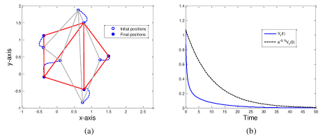
Figure 6: (a) Under control law (11), the agents asymptotically form a regular pentagon. (b) $V_{F}(t)$ vanishes to zero in an exponential speed.

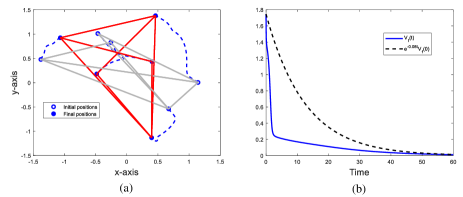
Figure 7: (a) Under control law (11), the agents with a set of random initial positions asymptotically form a shape distinct to regular pentagon. (b) $V_{F}(t)$ vanishes to zero in an exponential speed.

Example 31.

Consider the framework in Fig. 5 (b) as the target formation. According to (8), the set of desired angle information should be $\{g_{13}^{*T}g_{14}^{*}=0.8090,g_{14}^{*T}g_{15}^{*}=0.8090,g_{31}^{*T}g_{34}^{*}=0.3090,g_{41}^{*T}g_{45}^{*}=0.8090\}$. Under the same initial condition as in Example 30, although $V_{F}$ vanishes to zero exponentially, the control law (11) cannot stabilize the target formation, as shown in Fig. 8. This is because the angle constraints determined by $\mathcal{T}_{\mathcal{G}}^{F}$ are not sufficient to determine angle rigidity of the framework.

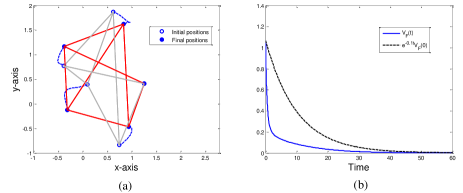
Figure 8: (a) Under control law (11), the agents asymptotically form a shape distinct to a regular pentagon. (b) $V_{F}(t)$ vanishes to zero in an exponential speed.

Example 32.

In this example, we control orientation and scale of the formation formed in Example 30 by implementing the control input (18). Let agents $3$ and $4$ be the two leaders. Now we aim to drive the direction of $p_{3}-p_{4}$ to be horizontal with respect to the global coordinate system, while setting the length of each edge as $0.5$. It suffices to set the target displacement between two leaders as $\tilde{p}_{3}-\tilde{p}_{4}=(-0.5,0)^{T}$. Fig. 9 shows the trajectories of agents and the evolution of $V(t)$ in (17), in which we can observe the validity of Theorem 29.

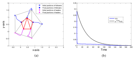
Figure 9: (a) Under control law (18), the regular pentagon formed by all agents is asymptotically transformed into another regular pentagon with desired orientation and scale. (b) $V(t)$ vanishes to zero exponentially.

6 Conclusion

In this paper, we have developed an angle rigidity theory to study when a framework in the plane can be determined by angles uniquely up to translations, rotations, scalings and reflections. We have also proved that the shape of a triangulated framework can always be uniquely determined by angles. On the basis of the proposed angle rigidity theory, a distributed formation controller has been designed for formation shape stabilization. We have proved that by implementing our control strategy, a formation containing a strongly nondegenerate triangulated framework is locally exponentially stable. Taking the advantage of high degrees of freedom, we have proposed a distributed control strategy, which can drive agents to stabilize a target formation shape with prescribed orientation and scale.

The angle rigidity theory proposed in this paper is only for graphs in the plane, similar definitions can be easily extended to higher dimensional spaces, but many properties of angle rigidity may become invalid. This is because many theoretical tools we have used cannot be directly applied to the higher dimensional case. We leave the angle rigidity theory in higher dimensional spaces as the future work. Moreover, the controller we presented requires agents to sense relative position states. We will try to design a bearing-only control law in future.

7 Appendix. A: Proof of Theorem 11

Necessity. Since $\operatorname{null}(R_{\mathcal{T}_{\mathcal{G}}^{*}})=(\operatorname{null}(R_{g})\cap\operatorname{range}(R_{B}))\cup\operatorname{null}(R_{B})$, $\dim(\operatorname{null}(R_{\mathcal{T}_{\mathcal{G}}^{*}}))$ reaches its minimum only if $\dim(\operatorname{null}(R_{B}))$ is minimal. Recall that it always holds that $\operatorname{null}(R_{B})\supseteq\mathcal{S}_{s}\cup\mathcal{S}_{t}$, once $(\mathcal{G},p)$ is infinitesimally angle rigid, it must hold that $\operatorname{null}(R_{B}(p))=\mathcal{S}_{s}\cup\mathcal{S}_{t}$. That is, $(\mathcal{G},p)$ is infinitesimally bearing rigid.

Sufficiency. Note that $R_{\mathcal{T}_{\mathcal{G}}^{*}}=R_{g}R_{B}$, and infinitesimal bearing rigidity implies $\operatorname{null}(R_{B})=\mathcal{S}_{t}\cup\mathcal{S}_{s}$. To show $\operatorname{null}(R_{\mathcal{T}_{\mathcal{G}}^{*}})=\mathcal{S}$, it suffices to show that for any $\eta\in\operatorname{null}(R_{g})\cap\operatorname{range}(R_{B})$, we have $\eta=R_{B}q$ for some $q\in\mathcal{S}_{r}$.

Suppose $\eta=R_{B}v$ and $R_{g}\eta=R_{g}R_{B}v=0$ for some $v=(v_{1}^{T},\cdots,v_{n}^{T})^{T}\in\mathbb{R}^{2n}$. Let $g_{ij}^{T}g_{ik}$ be a component of $f_{\mathcal{G}}$ such that $g_{ij}$ and $g_{ik}$ are not collinear. Then $R_{\mathcal{T}_{\mathcal{G}}^{*}}v=0$ implies that $\frac{\partial g_{ij}^{T}g_{ik}}{\partial g}\operatorname{diag}(\frac{P_{ij}}{||e_{ij}||})\bar{H}v=0$, which is equivalent to

$$e_{ik}^{T}P_{ij}(v_{i}-v_{j})+e_{ij}^{T}P_{ik}(v_{i}-v_{k})=0.$$ (20)

Note that for any nonzero vectors $x,y\in\mathbb{R}^{2}$, $P(x)y$ is perpendicular to $x$. Therefore, there always exist $c_{ij},c_{ik}\in\mathbb{R}$ such that

$$P_{ij}(v_{i}-v_{j})=c_{ij}\mathscr{R}_{o}(\frac{\pi}{2})g_{ij},~{}P_{ik}(v_{i}-v_{k})=c_{ik}\mathscr{R}_{o}(\frac{\pi}{2})g_{ik}.$$ (21)

It follows that

$$v_{i}-v_{j}=c_{ij}\mathscr{R}_{o}(\frac{\pi}{2})g_{ij}+c_{ij}^{\prime}g_{ij},~{}v_{i}-v_{k}=c_{ik}\mathscr{R}_{o}(\frac{\pi}{2})g_{ik}+c_{ik}^{\prime}g_{ik}$$ (22)

for some $c_{ij}^{\prime},c_{ik}^{\prime}\in\mathbb{R}$. Substituting (21) into (20), we have

$$c_{ij}e_{ik}^{T}\mathscr{R}_{o}(\frac{\pi}{2})g_{ij}+c_{ik}e_{ij}^{T}\mathscr{R}_{o}(\frac{\pi}{2})g_{ik}=0.$$

Note also that $\mathscr{R}_{o}^{T}(\frac{\pi}{2})=-\mathscr{R}_{o}(\frac{\pi}{2})$, then we have

$$(c_{ij}||e_{ik}||-c_{ik}||e_{ij}||)g_{ij}^{T}\mathscr{R}_{o}(\frac{\pi}{2})g_{ik}=0.$$

Since $g_{ij}$ and $g_{ik}$ are not collinear, $g_{ij}^{T}\mathscr{R}_{o}(\frac{\pi}{2})g_{ik}\neq 0$. It follows that $c_{ij}||e_{ik}||=c_{ik}||e_{ij}||$. That is, $c_{ij}=c_{ijk}||e_{ij}||$, $c_{ik}=c_{ijk}||e_{ik}||$ for some $c_{ijk}\in\mathbb{R}$. Together with (22), we have

$$\begin{split}&v_{i}-v_{j}=c_{ijk}\mathscr{R}_{o}(\frac{\pi}{2})e_{ij}+\bar{c}_{ij}e_{ij},\\ &v_{i}-v_{k}=c_{ijk}\mathscr{R}_{o}(\frac{\pi}{2})e_{ik}+\bar{c}_{ik}e_{ik},\end{split}$$ (23)

where $\bar{c}_{ij}=c_{ij}^{\prime}/||e_{ij}||$, $\bar{c}_{ik}=c_{ik}^{\prime}/||e_{ik}||$.

So far we have proved that if $(i,j,k)\in\mathcal{T}_{\mathcal{G}}^{*}$ and $g_{ij}$ is not collinear with $g_{ik}$, then (23) holds for some $c_{ijk}\in\mathbb{R}$. In the following, by constructing a $\mathcal{T}_{\mathcal{G}}^{*}$, we will show that there exists a common constant $c\in\mathbb{R}$ such that $v_{i}-v_{j}=c\mathscr{R}_{o}(\frac{\pi}{2})e_{ij}+\bar{c}_{ij}e_{ij}$ for all $(i,j)\in\mathcal{E}$.

Now we construct a set $\mathcal{T}_{\mathcal{G}}^{*}\subseteq\mathcal{T}_{\mathcal{G}}$ such that $g_{ij}$ and $g_{ik}$ are not collinear for all $(i,j,k)\in\mathcal{T}_{\mathcal{G}}^{*}$. Since $(\mathcal{G},p)$ is infinitesimally bearing rigid, from Lemma 1 and Lemma 2, for any vertex $i$, there exist at least two neighbors $j,k\in\mathcal{N}_{i}$ such that $g_{ij}$ and $g_{ik}$ are not collinear. As a result, we can divide $\mathcal{N}_{i}$ into two sets $\hat{\mathcal{N}}_{i}$ and $\check{\mathcal{N}}_{i}$, such that for any $j\in\hat{\mathcal{N}}_{i}$ and $k\in\check{\mathcal{N}}_{i}$, $g_{ij}$ and $g_{ik}$ are not collinear. We construct a set ${}^{i}\mathcal{T}_{\mathcal{G}}^{*}$ by the following two steps:

Step 1. Select a vertex $j_{1}\in\hat{\mathcal{N}}_{i}$ randomly, let $(i,j_{1},k)$(if $j_{1}<k$) or $(i,k,j_{1})$(if $j_{1}>k$) for all $k\in\check{\mathcal{N}}_{i}$ be an element of ${}^{i}\mathcal{T}_{\mathcal{G}}^{*}$.

Step 2. Select a vertex $k_{1}\in\check{\mathcal{N}}_{i}$ randomly, let $(i,j,k_{1})$(if $j<k_{1}$) or $(i,k_{1},j)$(if $j>k_{1}$) for all $j\in\hat{\mathcal{N}}_{i}\setminus\{j_{1}\}$ be an element of ${}^{i}\mathcal{T}_{\mathcal{G}}^{*}$.

Let $\mathcal{T}_{\mathcal{G}}^{*}=\cup_{i\in\mathcal{V}}~{}^{i}\mathcal{T}_{\mathcal{G}}^{*}$. It is obvious that for any $i,j,k\in\mathcal{T}_{\mathcal{G}}^{*}$, $g_{ij}$ and $g_{ik}$ are not collinear. Now we regard each edge $(i,j)$ of $\mathcal{G}$ as a vertex of $\mathcal{G}^{\prime}$, $(i,j)$ and $(i,k)$ are adjacent if $(i,j,k)$ or $(i,k,j)$ belongs to $\mathcal{T}_{\mathcal{G}}^{*}$. By our approach for construction of ${}^{i}\mathcal{T}_{\mathcal{G}}^{*}$, it is easy to see that for any $i\in\mathcal{V}$ and $j,k\in\mathcal{N}_{i}$, $(i,j)$ and $(i,k)$ are either adjacent or both neighbors of $(i,j_{1})$ or $(i,k_{1})$. Therefore, the graph $\mathcal{G}^{\prime}$ corresponding to $\mathcal{T}_{\mathcal{G}}^{*}$ is connected. We regard $c_{ij}$ as the state corresponding to $(i,j)$ if $v_{i}-v_{j}=c_{ij}\mathscr{R}_{o}(\frac{\pi}{2})e_{ij}+\bar{c}_{ij}e_{ij}$. Note that (23) implies that if $(i,j)$ and $(i,k)$ are adjacent, they share a common state $c_{ijk}\in\mathbb{R}$. Since $\mathcal{G}^{\prime}$ is connected, all edges in $\mathcal{G}^{\prime}$ have a consensus state $c\in\mathbb{R}$. That is, $v_{i}-v_{j}=c\mathscr{R}_{o}(\frac{\pi}{2})e_{ij}+\bar{c}_{ij}e_{ij}$ for all $(i,j)\in\mathcal{E}$.

This implies that $\bar{H}v=c(I_{m}\otimes\mathscr{R}_{o}(\frac{\pi}{2}))\bar{H}p+\bar{C}\bar{H}p$, where $\bar{C}=\operatorname{diag}(\bar{c}_{ij})\otimes I_{2}$. Then

$$\begin{split}\eta&=R_{B}v=\operatorname{diag}(\frac{P_{ij}}{||e_{ij}||})\bar{H}v\\ &=\operatorname{diag}(\frac{P_{ij}}{||e_{ij}||})c(I_{m}\otimes\mathscr{R}_{o}(\frac{\pi}{2}))(H\otimes I_{2})p+\operatorname{diag}(\frac{P_{ij}}{||e_{ij}||})\bar{C}\bar{H}p\\ &=\operatorname{diag}(\frac{P_{ij}}{||e_{ij}||})(H\otimes I_{2})c(I_{n}\otimes\mathscr{R}_{o}(\frac{\pi}{2}))p\\ &=R_{B}c(I_{n}\otimes\mathscr{R}_{o}(\frac{\pi}{2}))p.\end{split}$$

Since $c(I_{n}\otimes\mathscr{R}_{o}(\frac{\pi}{2}))p\in\mathcal{S}_{r}$, the proof is completed.

8 Appendix. B: Proof of Theorem 14

We first present some lemmas that are required to prove Theorem 14.

In [9], the authors showed that for a positive semi-definite matrix $A\in\mathbb{R}^{n\times n}$ with $\operatorname{rank}(A)=r$, if $\Pi^{T}A\Pi=R^{T}R$ for a specified permutation matrix $\Pi\in\mathbb{R}^{n\times n}$, where $R\in\mathbb{R}^{r\times n}$, then this Cholesky decomposition is unique. Here the uniqueness of Cholesky decomposition implies that if $\bar{R}^{T}\bar{R}=\Pi^{T}A\Pi$ for some $\bar{R}\in\mathbb{R}^{r\times n}$, then $R=\mathscr{R}\bar{R}$ for some $\mathscr{R}\in\textrm{O(2)}$. It is straightforward to obtain the following lemma.

Lemma 33.

For a matrix $R\in\mathbb{R}^{r\times n}$ with $\operatorname{rank}(R)=r$, if $R^{T}R=\bar{R}^{T}\bar{R}$ for some $\bar{R}\in\mathbb{R}^{r\times n}$, then $R=\mathscr{R}\bar{R}$ for some $\mathscr{R}\in O(r)$.

Let $\mathscr{H}_{x}=\mathscr{H}(x)\triangleq I_{2}-2xx^{T}$ be a Householder transformation, here $x\in\mathbb{R}^{2}$ is a unit vector. Geometrically, $\mathscr{H}_{x}y$ with $y\in\mathbb{R}^{2}$ is a reflection of $y$ about the vector which is perpendicular to $x$. We list some properties of $\mathscr{H}_{x}$ in the following lemma.

Lemma 34.

For any given unit vectors $x,y\in\mathbb{R}^{2}$, $\mathscr{H}_{x}$ has the following properties:

(i) $\mathscr{H}_{x}^{T}=\mathscr{H}$, $\mathscr{H}_{x}^{2}=I_{2}$;

(ii) $\mathscr{H}_{x}=\mathscr{R}_{e}(\theta)$ for some $\theta\in[0,2\pi)$;

(iii) For any $\theta\in[0,2\pi)$, there exists a unit vector $z\in\mathbb{R}^{2}$ such that $\mathscr{H}_{z}=\mathscr{R}_{e}(\theta)$;

(iv) The eigenspace of $\mathscr{H}_{x}$ associated with the eigenvalue 1 is $\operatorname{span}\{x^{\perp}\}$.

Proof. The statements in (i) and (ii) are easy to verify, thus the proofs are omitted here. Now we prove the rest of statements.

(iii) Let $x=(x_{1},x_{2})^{T}$, then $H_{x}=I-2xx^{T}=\begin{pmatrix}1-2x_{1}^{2}~{}~{}&-2x_{1}x_{2}\\ -2x_{1}x_{2}~{}~{}&1-2x_{2}^{2}\end{pmatrix}$. It suffices to show that $1-2x_{1}^{2}=-(1-2x_{2}^{2})$ and $(1-2x_{1}^{2})^{2}+(-2x_{1}x_{2})^{2}=1$. Since $x_{1}^{2}+x_{2}^{2}=1$, the first equality obviously holds. For the second equality, we have

$$\begin{split}(1-2x_{1}^{2})^{2}+(-2x_{1}x_{2})^{2}&=1-4x_{1}^{2}+4x_{1}^{4}+4x_{1}^{2}x_{2}^{2}\\ &=1-4x_{1}^{2}+4x_{1}^{2}(x_{1}^{2}+x_{2}^{2})=1.\end{split}$$

(iv) From the proof for (iii), it suffices to find suitable $x$ such that $1-2x_{1}^{2}=\cos\theta$, $1-2x_{2}^{2}=-\cos\theta$, and $-2x_{1}x_{2}=\sin\theta$. If $\theta\in[0,\pi)$, we can obtain a solution as $x_{1}=\sqrt{\frac{1-\cos\theta}{2}}$, $x_{2}=-\sqrt{\frac{1-\cos\theta}{2}}$. If $\theta\in[\pi,2\pi)$, a solution is $x_{1}=\sqrt{\frac{1-\cos\theta}{2}}$, $x_{2}=\sqrt{\frac{1-\cos\theta}{2}}$.

(v) Let $y\in\mathbb{R}^{2}$ be a vector such that $H_{x}y=y$, then $y-2x^{T}yx=y$, which holds if and only if $x^{T}y=0$, i.e., $y=cx^{\perp}$ for some constant $c\in\mathbb{R}$. $\square$

With the aid of Lemma 34, we can establish the following result.

Lemma 35.

If $A\eta=B\eta$, where $A,B\in\textrm{O(2)}$, and $\eta\in\mathbb{R}^{2}$ is a unit vector, then $A=B$ or $A=B\mathscr{H}_{\eta^{\perp}}$.

Proof. Note that a 2-dimensional orthogonal matrix is either a rotation matrix or a reflection matrix. Without loss of generality, we discuss the problem in three cases:

Case 1. $A=\mathscr{R}_{o}(\alpha)$, $B=\mathscr{R}_{o}(\beta)$ for some $\alpha,\beta\in[0,2\pi)$. Then $\mathscr{R}_{o}(\alpha)\eta=\mathscr{R}_{o}(\beta)\eta$, implying $\mathscr{R}_{o}(\alpha-\beta)\eta=\eta$. Hence $\alpha-\beta=0$. That is, $A=B$.

Case 2. $A=\mathscr{R}_{e}(\alpha)$, $B=\mathscr{R}_{e}(\beta)$ for some $\alpha,\beta\in[0,2\pi)$. Following the same procedure in Case 1, one can also obtain $A=B$.

Case 3. $A=\mathscr{R}_{o}(\alpha)$, $B=\mathscr{R}_{e}(\beta)=\mathscr{R}_{o}(\beta)\bar{I}$ for some $\alpha,\beta\in[0,2\pi)$. Then $\mathscr{R}_{o}(\alpha)\eta=\mathscr{R}_{o}(\beta)\bar{I}\eta$. It follows that $\eta=\mathscr{R}_{o}(\beta-\alpha)\bar{I}\eta=\mathscr{R}_{e}(\beta-\alpha)\eta$. From Lemma 34 (iii), there exists some $x\in\mathbb{R}^{2}$ such that $\mathscr{H}_{x}=\mathscr{R}_{e}(\beta-\alpha)$. That is, $\eta=\mathscr{H}_{x}\eta$. Using (iv) in Lemma 34, we have $\eta\in\operatorname{span}\{x^{\perp}\}$. Then $x=\pm\eta^{\perp}$, $\mathscr{H}_{x}=\mathscr{H}_{\eta^{\perp}}$. As a result, $\mathscr{H}_{\eta^{\perp}}=\mathscr{R}_{e}(\beta-\alpha)=\mathscr{R}_{o}(\beta-\alpha)\bar{I}$, implying that $\mathscr{R}_{o}(\alpha)\mathscr{H}_{\eta^{\perp}}=\mathscr{R}_{e}(\beta)$. By (i) in Lemma 34, we have $A=\mathscr{R}_{o}(\alpha)=\mathscr{R}_{e}(\beta)\mathscr{H}_{\eta^{\perp}}=B\mathscr{H}_{\eta^{\perp}}$. $\square$

Let $\mathcal{F}$ denote a graph with $4$ vertices and 5 edges, then the following lemma holds.

Lemma 36.

$(\mathcal{F},p)$ is infinitesimally bearing rigid if and only if $p$ is nondegenerate.

The necessity of Lemma 36 is obvious. For sufficiency, it is easy to see that $\mathcal{F}$ must be a triangulated Laman graph. Since $(\mathcal{L}_{4},p)$ is strongly nondegenerate if and only if $p$ is nondegenerate, from Lemma 20, $(\mathcal{L}_{4},p)$ is infinitesimally distance rigid.

With Lemmas 33, 34, 35 and 36 at hand, we now give the proof for Theorem 14.

Proof of Theorem 14. We first note that $(I_{n}\otimes\mathscr{R})^{-1}q\in~{}B_{\mathcal{K}}^{-1}(B_{\mathcal{K}}(p))$ is equivalent to $B_{\mathcal{K}}((I_{n}\otimes\mathscr{R})^{-1}q)=~{}B_{\mathcal{K}}(p)$, which is also equivalent to $B_{\mathcal{K}}(q)=(I_{m}\otimes\mathscr{R})B_{\mathcal{K}}(p)$. Therefore, it suffices to show that $f_{\mathcal{K}}(q)=f_{\mathcal{K}}(p)$ if and only if $B_{\mathcal{K}}(q)=(I_{m}\otimes\mathscr{R})B_{\mathcal{K}}(p)$.

Sufficiency. For any $i,j,k\in\mathcal{V}$, it is straightforward that

$$g_{ij}^{T}(q)g_{ik}(q)=g_{ij}^{T}(p)\mathscr{R}^{T}\mathscr{R}g_{ik}(p)=g_{ij}^{T}(p)g_{ik}(p).$$

To prove necessity, we consider the following two cases.

Case 1. The configuration $p$ is degenerate. Let $\tilde{g}$ be a unit vector such that $\tilde{g}$ is collinear with $g_{ij}(p)$ for all $i,j\in\mathcal{V}$, then $g_{ij}(q)=\mathscr{R}g_{ij}(p)$ if and only if $g_{ij}(q)=\mathscr{R}\mathscr{H}_{\tilde{g}^{\perp}(p)}g_{ij}(p)$. For any $i,j\in\mathcal{V}$, let $\mathscr{R}_{ij}\in\textrm{O(2)}$ such that $g_{ij}(q)=\mathscr{R}_{ij}g_{ij}(p)$. To prove necessity, it suffices to show that for any distinct vertices $i,j,k\in\mathcal{V}$, if $g_{ij}(q)=\mathscr{R}_{ij}g_{ij}(p)$ and $g_{ik}(q)=\mathscr{R}_{ik}g_{ik}(p)$, there always holds $\mathscr{R}_{ij}=\mathscr{R}_{ik}$ or $\mathscr{R}_{ij}=\mathscr{R}_{ik}\mathscr{H}_{\tilde{g}^{\perp}(p)}$. Without loss of generality, suppose $g_{ij}(p)=g_{ik}(p)$. Then $g_{ij}^{T}(q)g_{ik}(q)=g_{ij}^{T}(p)g_{ik}(p)=1$, which holds if and only if $g_{ij}(q)=g_{ik}(q)$, i.e., $\mathscr{R}_{ij}g_{ij}(p)=\mathscr{R}_{ik}g_{ik}(p)=\mathscr{R}_{ik}g_{ij}(p)$. By Lemma 35, $\mathscr{R}_{ij}=\mathscr{R}_{ik}$ or $\mathscr{R}_{ij}=\mathscr{R}_{ik}\mathscr{H}_{g_{ij}^{\perp}(p)}$. Since $\mathscr{H}_{g_{ij}^{\perp}(p)}=\mathscr{H}_{\tilde{g}^{\perp}(p)}$, the proof is completed.

Case 2. The configuration $p$ is nondegenerate. Note that $\mathcal{K}$ is complete, hence each vertex $i$ has at least two neighbors $j$ and $k$ such that $g_{ij}(p)$ and $g_{ik}(p)$ are not collinear. Then we can divide $\mathcal{N}_{i}$ into two sets $\hat{\mathcal{N}}_{i}$ and $\check{\mathcal{N}}_{i}$, such that for any $j\in\hat{\mathcal{N}}_{i}$ and $k\in\check{\mathcal{N}}_{i}$, $g_{ij}(p)$ and $g_{ik}(p)$ are not collinear. We first show that given $i\in\mathcal{V}$, for any $j\in\hat{\mathcal{N}}_{i}$, $k\in\check{\mathcal{N}}_{i}$, $l\in\mathcal{V}\setminus\{i,j,k\}$, it always holds that $G_{ijkl}(q)=\mathscr{R}_{ijkl}G_{ijkl}(p)$ for some $\mathscr{R}_{ijkl}\in\textrm{O(2)}$, where $G_{ijkl}=(g_{ij},g_{ik},g_{il},g_{jk},g_{jl},g_{kl})\in\mathbb{R}^{2\times 6}$.

Since $\mathcal{K}$ is complete, we have $l\in\mathcal{N}_{i}$. Without loss of generality, we consider $l\in\check{\mathcal{N}}_{i}$. For the triangle composed of $i,j,k$, let $G_{ijk}=(g_{ij},g_{ik},g_{jk})\in\mathbb{R}^{2\times 3}$. Since $f_{\mathcal{K}}(q)=~{}f_{\mathcal{K}}(p)$, we have $G_{ijk}^{T}(q)G_{ijk}(q)=G_{ijk}^{T}(p)G_{ijk}(p)$. Note that $g_{ij}(p)$ and $g_{ik}(p)$ are not collinear, thus we have $\operatorname{rank}(G_{ijk}(p))=2$. By virtue of Lemma 33, the Cholesky decomposition of $G_{ijk}^{T}(p)G_{ijk}(p)$ determines $G_{ijk}(p)$ up to a $2\times 2$ orthogonal matrix $\mathscr{R}_{ijk}$. That is, $G_{ijk}(q)=\mathscr{R}_{ijk}G_{ijk}(p)$. Similarly, we have $G_{ijl}(q)=\mathscr{R}_{ijl}G_{ijl}(p)$ for $\mathscr{R}_{ijl}\in\textrm{O(2)}$. For vertices $j,k,l$, it follows from Case 1 that $G_{jkl}(q)=\mathscr{R}_{jkl}G_{jkl}(p)$ for $\mathscr{R}_{jkl}\in\textrm{O(2)}$ no matter $j,k,l$ are collinear or not. Since $\mathscr{R}_{ijk}g_{ij}(p)=\mathscr{R}_{ijl}g_{ij}(p)=g_{ij}(q)$, according to Lemma 35, $\mathscr{R}_{ijk}=\mathscr{R}_{ijl}$ or $\mathscr{R}_{ijk}=\mathscr{R}_{ijl}\mathscr{H}_{g_{ij}^{\perp}(p)}$.

Suppose that $\mathscr{R}_{ijk}\neq\mathscr{R}_{ijl}$, then

$$\begin{split}g_{jk}^{T}(p)g_{jl}(p)&=g_{jk}^{T}(q)g_{jl}(q)\\ &=g^{T}_{jk}(p)\mathscr{R}_{ijk}^{T}\mathscr{R}_{ijl}g_{jl}(p)\\ &=g^{T}_{jk}(p)\mathscr{H}_{g_{ij}^{\perp}(p)}g_{jl}(p)\\ &=g^{T}_{jk}(p)g_{jl}(p)-2g^{T}_{jk}(p)g_{ij}^{\perp}(p)g_{ij}^{\perp T}(p)g_{jl}(p).\end{split}$$

This implies $g^{T}_{jk}(p)g_{ij}^{\perp}(p)g_{ij}^{\perp T}(p)g_{jl}(p)=0$. Since $g_{ij}(p)$ and $g_{ik}(p)$ are not collinear, $g_{ij}(p)$ and $g_{jk}(p)$ are also not collinear. Similarly, $g_{ij}(p)$ and $g_{jl}(p)$ are not collinear. Thus a contradiction arises. We then have $\mathscr{R}_{ijk}=\mathscr{R}_{ijl}\triangleq\mathscr{R}_{ijkl}$, which implies that $\bar{G}_{ijkl}(q)=\mathscr{R}_{ijkl}\bar{G}_{ijkl}(p)$, where $\bar{G}_{ijkl}=(g_{ij},g_{ik},g_{il},g_{jk},g_{jl})\in\mathbb{R}^{2\times 5}$. Consider the framework $(\mathcal{F},q)$, where $\mathcal{F}$ is a graph with vertex set $\{i,j,k,l\}$ and edge set $\{(i,j),(i,k),(i,l),(j,k),(k,l)\}$. Since these four vertices are not collinear, according to Lemma 36, $(\mathcal{F},q)$ is infinitesimally bearing rigid, thus is globally bearing rigid. This implies that $g_{kl}(q)$ can be uniquely determined by $\bar{G}_{ijkl}(q)$. As a result, $G_{ijkl}(q)=\mathscr{R}_{ijkl}G_{ijkl}(p)$.

The above proof implies that given $i\in\mathcal{V}$, we have

$$\mathscr{R}\triangleq\mathscr{R}_{ijk}=\mathscr{R}_{ijl}=\mathscr{R}_{ikl}=\mathscr{R}_{jkl}$$

for any $j\in\hat{\mathcal{N}}_{i}$, $k\in\check{\mathcal{N}}_{i}$, $l\in\mathcal{V}\setminus\{i,j,k\}$. Note that any edge in graph $\mathcal{K}$ is involved in a triangle including vertex $i$. Therefore, $g_{ij}(q)=\mathscr{R}g_{ij}(p)$ for any $(i,j)\in\mathcal{E}$. $\square$

9 Appendix. C: Proof of Theorem 21

(i) From Lemma 20 and the fact that $|\mathcal{E}_{n}|=2n-3$, strong nondegeneracy and minimal infinitesimal angle rigidity are equivalent for $(\mathcal{L}_{n},p)$. Next we show $\mathcal{T}_{\mathcal{L}_{n}}^{*}$ in (6) is minimally suitable for $(\mathcal{L}_{n},p)$ to be minimally infinitesimally angle rigid.

By virtues of Theorem 11 and Lemma 20, $(\mathcal{L}_{n},p)$ is infinitesimally bearing rigid. Then $\operatorname{null}(R_{B})=\mathcal{S}_{s}\cup\mathcal{S}_{t}$. It suffices to show that for any $\eta\in\operatorname{null}(R_{g})\cap\operatorname{range}(R_{B})$, there always exists $q\in\mathcal{S}_{r}$ such that $\eta=R_{B}q$. Suppose that $R_{\mathcal{T}_{\mathcal{L}_{n}}^{*}}v=R_{g}R_{B}v=0$ and $R_{B}v\neq 0$, where $v=(v_{1}^{T},\cdots,v_{n}^{T})\in\mathbb{R}^{2n}$. In the proof of Theorem 11, we have shown that for any $(i,j,k)\in\mathcal{T}_{\mathcal{L}_{n}}^{*}$, if $g_{ij}$ is not collinear with $g_{ik}$, then (23) holds for some $c_{ijk}$. Recall that $(\mathcal{L}_{n},p)$ is strongly nondegenerate, then for any $(i,j,k)\in\mathcal{T}_{\mathcal{L}_{n}}^{*}$, (23) holds for some $c_{ijk}$. Without loss of generality, suppose $i<j<k$. Due to the definition in (6), for each triangle in $\mathcal{L}_{n}$ formed by vertices $i$, $j$ and $k$, we have $(i,j,k),(j,i,k)\in\mathcal{T}_{\mathcal{L}_{n}}^{*}$. Now we regard $(i,j)$ as a vertex of $\mathcal{G}^{\prime}$ for all $(i,j)\in\mathcal{E}_{n}$, two vertices in $\mathcal{G}^{\prime}$ are adjacent if they belong to a same triangle in $\mathcal{L}_{n}$. Let $c_{ij}$ be the state of $(i,j)$ if $v_{i}-v_{j}=c_{ij}\mathscr{R}_{o}(\frac{\pi}{2})e_{ij}+\bar{c}_{ij}e_{ij}$ for some $\bar{c}_{ij}\in\mathbb{R}$. It is easy to see that $(i,j)$, $(i,k)$ and $(k,j)$ have a common state, implying that adjacent vertices in $\mathcal{G}^{\prime}$ must have a common state. Note that in every step during the generation of graph $\mathcal{L}_{n}$, a new triangle is generated based on an existing edge. Therefore, $\mathcal{G}^{\prime}$ must be connected. As a result, there exists a constant $c\in\mathbb{R}$ such that $v_{i}-v_{j}=c\mathscr{R}_{o}(\frac{\pi}{2})e_{ij}+\bar{c}_{ij}e_{ij}$ for all $(i,j)\in\mathcal{E}_{n}$. By similar analysis to the proof of Theorem 11, we can obtain $v\in\mathcal{S}_{r}$, which implies that $(\mathcal{L}_{n},p)$ is infinitesimally angle rigid for $\mathcal{T}_{\mathcal{L}_{n}}^{*}$. Moreover, observe that $|\mathcal{T}_{\mathcal{L}_{n}}^{*}|=2n-4$, we conclude that $\mathcal{T}_{\mathcal{L}_{n}}^{*}$ is also minimal.

(ii). We prove the statement by induction.

For $n=3$, it is obvious that $(\mathcal{L}_{3},p)$ with $\mathcal{T}_{\mathcal{L}_{3}}^{\dagger}=\mathcal{T}_{\mathcal{L}_{3}}^{*}=\{(1,2,3),(2,1,3)\}$ is globally angle rigid.

For $n\geq 4$, suppose that $(\mathcal{L}_{n-1},p)$ with $\mathcal{T}_{\mathcal{L}_{n-1}}^{\dagger}$ is globally angle rigid. Next we show that $(\mathcal{L}_{n},p)$ is globally angle rigid with $\mathcal{T}_{\mathcal{L}_{n}}^{\dagger}$. Without loss of generality, let $i$ and $j$ be the neighbors of $n$ and $i<j$. Note that $(i,j)\in\mathcal{E}_{n-1}$, and $i$, $j$ must have at least one common neighbor vertex in $\mathcal{L}_{n-1}$, let $k$ be the minimum index among them, it is easy to see $\mathcal{T}_{\mathcal{L}_{n}}^{\dagger}=\{(i,j,n),(j,i,n),(i,k,n)\}\cup\mathcal{T}_{\mathcal{L}_{n-1}}^{\dagger}$. It suffices to show that for any $q$ such that $f_{\mathcal{T}_{\mathcal{L}_{n}}^{\dagger}}(p)=f_{\mathcal{T}_{\mathcal{L}_{n}}^{\dagger}}(q)$, it always holds $f_{\mathcal{K}_{n}}(p)=f_{\mathcal{K}_{n}}(q)$. Since $\mathcal{L}_{n-1}$ is globally angle rigid, by Theorem 14, there exists a matrix $\mathscr{R}_{n-1}\in\textrm{O(2)}$ such that $g_{i^{\prime}j^{\prime}}(p)=\mathscr{R}_{n-1}g_{i^{\prime}j^{\prime}}(q)$ for all $i^{\prime},j^{\prime}\in\mathcal{V}_{n-1}$. From $g_{ij}^{T}(p)g_{in}(p)=g_{ij}^{T}(q)g_{in}(q)$, and $g_{ji}^{T}(p)g_{jn}(p)=g_{ji}^{T}(q)g_{jn}(q)$, we have $G_{ijn}^{T}(p)G_{ijn}(p)=G_{ijn}^{T}(q)G_{ijn}(q)$, where $G_{ijn}=(g_{ij},g_{nj},g_{ni})\in\mathbb{R}^{2\times 3}$. Using strong nondegeneracy of $(\mathcal{L}_{n},p)$, we have $\operatorname{rank}(G_{ijn}(p))=2$. By Lemma 33, $G_{ijn}(p)=\mathscr{R}_{ijn}G_{ijn}(q)$ for some $\mathscr{R}_{ijn}\in\textrm{O(2)}$. It follows that $g_{ij}(p)=\mathscr{R}_{n-1}g_{ij}(q)=\mathscr{R}_{ijn}g_{ij}(q)$. According to Lemma 35, $\mathscr{R}_{n-1}=\mathscr{R}_{ijn}$ or $\mathscr{R}_{n-1}=\mathscr{R}_{ijn}\mathscr{H}_{g_{ij}^{\perp}(q)}$.

Suppose that $\mathscr{R}_{n-1}\neq\mathscr{R}_{ijn}$, then $g_{ik}(p)=\mathscr{R}_{n-1}g_{ik}(q)=\mathscr{R}_{ijn}\mathscr{H}_{g_{ij}^{\perp}(q)}g_{ik}(q)$, and $g_{in}(p)=\mathscr{R}_{ijn}g_{in}(q)$. It follows that

$$\begin{split}g_{ik}^{T}(p)g_{in}(p)&=g_{ik}^{T}(q)\mathscr{H}_{g_{ij}^{\perp}(q)}\mathscr{R}_{ijn}^{T}\mathscr{R}_{ijn}g_{in}(q)\\ &=g_{ik}^{T}(q)\mathscr{H}_{g_{ij}^{\perp}(q)}g_{in}(q).\end{split}$$ (24)

Recall that $(i,k,n)\in\mathcal{T}_{\mathcal{L}_{n}}^{\dagger}$, we have $g_{ik}^{T}(p)g_{in}(p)=g_{ik}^{T}(q)g_{in}(q)$. Together with (24), it follows that $g_{ik}^{T}(q)\mathscr{H}_{g_{ij}^{\perp}(q)}g_{in}(q)=g_{ik}^{T}(q)g_{in}(q)$, which holds if and only if $g_{ij}(q)$ is collinear with either $g_{ik}(q)$ or $g_{in}(q)$, i.e., either $(q_{i}^{T},q_{j}^{T},q_{k}^{T})^{T}$ or $(q_{i}^{T},q_{j}^{T},q_{n}^{T})^{T}$ is degenerate, implying that either $(p_{i}^{T},p_{j}^{T},p_{k}^{T})^{T}$ or $(p_{i}^{T},p_{j}^{T},p_{n}^{T})^{T}$ is degenerate. This conflicts with strong nondegeneracy of $(\mathcal{L}_{n},p)$. Therefore, $\mathscr{R}_{n-1}=\mathscr{R}_{ijn}\triangleq\mathscr{R}_{n}$. That is, $g_{i^{\prime}j^{\prime}}(p)=\mathscr{R}_{n}g_{i^{\prime}j^{\prime}}(q)$ for any $(i^{\prime},j^{\prime})\in\mathcal{E}_{n}$. It follows that $f_{\mathcal{K}}(p)=~{}f_{\mathcal{K}}(q)$. Hence, $(\mathcal{L}_{n},p)$ with $\mathcal{T}_{\mathcal{L}_{n}}^{*}$ is globally angle rigid.

References

- [1] B. D. O. Anderson, C. Yu, B. Fidan, and J. Hendrickx. Rigid graph control architectures for autonomous formations. IEEE Control Systems Magazine, 28(6):48–63, 2008.
- [2] M. Aranda, G. López-Nicolás, C. Sagüés, and M. M. Zavlanos. Distributed formation stabilization using relative position measurements in local coordinates. IEEE Transactions on Automatic Control, 61(12):3925–3935, 2016.
- [3] L. Asimow and B. Roth. The rigidity of graphs. Transactions of the American Mathematical Society, 245:279–289, 1978.
- [4] A. N. Bishop, I. Shames, and B. D. O. Anderson. Stabilization of rigid formations with direction-only constraints. In in Proceedings of the 50th IEEE Conference on Decision and Control and European Control Conference, Orlando, FL, pages 746–752, 2011.
- [5] I. Buckley and M. Egerstedt. Infinitesimally shape-similar motions using relative angle measurements. In in Proceedings of IEEE/RSJ International Conference on Intelligent Robots and Systems, Vancouver, BC, Canada, pages 1077–1082, 2017.
- [6] J. Carr. Applications of centre manifold theory. Springer-Verlag, New York, 1981.
- [7] X. Chen, M. A. Belabbas, and T. Başar. Global stabilization of triangulated formations. SIAM Journal on Control and Optimization, 55(1):172–199, 2017.
- [8] S. Coogan and M. Arcak. Scaling the size of a formation using relative position feedback. Automatica, 48(10):2677–2685, 2012.
- [9] J. J. Dongarra, C. B. Moler, J. R. Bunch, and G. W. Stewart. LINPACK users’ guide. SIAM, Philadelphia, 1979.
- [10] T. Eren. Formation shape control based on bearing rigidity. International Journal of Control, 85(9):1361–1379, 2012.
- [11] T. Eren, W. Whiteley, A. S. Morse, P. N. Belhumeur, and B. D. O. Anderson. Sensor and network topologies of formations with direction, bearing, and angle information between agents. In Proceedings of the 42nd IEEE Conference on Decision and Control, pages 3064–3069, 2003.
- [12] J. A. Fax and R. M. Murray. Information flow and cooperative control of vehicle formations. IEEE Transactions on Automatic Control, 49(9):1465–1476, 2004.
- [13] B. Hendrickson. Conditions for unique graph realizations. SIAM Journal on Computing, 21(1):65–84, 1992.
- [14] G. Jing, G. Zhang, H. W. Lee, and L. Wang. Weak rigidity theory and its application to formation stabilization. SIAM Journal on Control and Optimization, 56(3):2248–2273, 2018.
- [15] G. Jing, Y. Zheng, and L. Wang. Consensus of multiagent systems with distance-dependent communication networks. IEEE Transactions on Neural Networks and Learning Systems, 28:2712–2726, 2016.
- [16] L. Krick, M. E. Broucke, and B. A. Francis. Stabilization of infinitesimally rigid formations of multi-robot networks. International Journal of Control, 82(3):423–439, 2009.
- [17] J. Lee. Introduction to smooth manifolds. Springer, New York, 2000.
- [18] L. Liberti, C. Lavor, N. Maculan, and A. Mucherino. Euclidean distance geometry and applications. SIAM Review, 56(1):3–69, 2014.
- [19] Z. Lin, L. Wang, Z. Chen, M. Fu, and Z. Han. Necessary and sufficient graphical conditions for affine formation control. IEEE Transactions on Automatic Control, 61(10):2877–2891, 2016.
- [20] G. Michieletto, A. Cenedese, and A. Franchi. Bearing rigidity theory in se (3). In in Proceedings of the 55th IEEE Conference on Decision and Control, Las Vegas, USA, pages 5950–5955, 2016.
- [21] S. Mou, M. A. Belabbas, A. S. Morse, Z. Sun, and B. D. O. Anderson. Undirected rigid formations are problematic. IEEE Transactions on Automatic Control, 61(10):2821–2836, 2016.
- [22] K. K. Oh and H. S. Ahn. Formation control of mobile agents based on inter-agent distance dynamics. Automatica, 47(10):2306–2312, 2011.
- [23] K. K. Oh, M. C. Park, and H. S. Ahn. A survey of multi-agent formation control. Automatica, 53:424–440, 2015.
- [24] R. Olfati-Saber, J. A. Fax, and R. M. Murray. Consensus and cooperation in networked multi-agent systems. Proceedings of the IEEE, 95(1):215–233, 2007.
- [25] W. Ren and E. Atkins. Distributed multi-vehicle coordinated control via local information exchange. International Journal of Robust and Nonlinear Control, 17(10-11):1002–1033, 2007.
- [26] F. Schiano, A. Franchi, D. Zelazo, and P. R. Giordano. A rigidity-based decentralized bearing formation controller for groups of quadrotor uavs. In in Proceedings of IEEE/RSJ International Conference on Intelligent Robots and Systems, Daejeon, Korea, pages 5099–5106, 2016.
- [27] T. H. Summers, C. Yu, S. Dasgupta, and B. D. O. Anderson. Control of minimally persistent leader-remote-follower and coleader formations in the plane. IEEE Transactions on Automatic Control, 56(12):1255–1268, 2011.
- [28] Z. Sun, M. C. Park, B. D. O. Anderson, and H. S. Ahn. Distributed stabilization control of rigid formations with prescribed orientation. Automatica, 78:250–257, 2017.
- [29] L. Wang, H. Shi, T. Chu, W. Zhang, and L. Zhang. Aggregation of foraging swarms. Lecture Notes in Artificial Intelligence, 3339:766–777, 2004.
- [30] L. Wang and F. Xiao. Finite-time consensus problems for networks of dynamic agents. IEEE Transactions on Automatic Control, 55(4):950–955, 2007.
- [31] L. Wang and F. Xiao. A new approach to consensus problems in discrete-time multiagent systems with time-delays. Science in China Series F: Information Sciences, 50(4):625–635, 2007.
- [32] F. Xiao, L. Wang, J. Chen, and Y. Gao. Finite-time formation control for multi-agent systems. Automatica, 45(11):2605–2611, 2009.
- [33] C. Yu, B. D. O. Anderson, S. Dasgupta, and B. Fidan. Control of minimally persistent formations in the plane. SIAM Journal on Control and Optimization, 48(1):206–233, 2009.
- [34] D. Zelazo, A. Franchi, H. H. Bülthoff, and P. Robuffo Giordano. Decentralized rigidity maintenance control with range measurements for multi-robot systems. The International Journal of Robotics Research, 34(1):105–128, 2015.
- [35] D. Zelazo, A. Franchi, and P. R. Giordano. Rigidity theory in se(2) for unscaled relative position estimation using only bearing measurements. In in Proceedings of European Control Conference, Strasbourg, France, pages 2703–2708, 2014.
- [36] D. Zelazo, P. R. Giordano, and A. Franchi. Bearing-only formation control using an se(2) rigidity heory. In in Proceedings of the 54th IEEE Conference on Decision and Control, Osaka, Japan, pages 6121–6126, 2015.
- [37] S. Zhao, F. Lin, K. Peng, B. M. Chen, and T. H. Lee. Distributed control of angle-constrained cyclic formations using bearing-only measurements. Systems & Control Letters, 63:12–24, 2014.
- [38] S. Zhao, Z. Sun, D. Zelazo, M. Trinh, and H. Ahn. Laman graphs are generically bearing rigid in arbitrary dimensions. Arxiv preprint: 1703.04035, 2017.
- [39] S. Zhao and D. Zelazo. Bearing rigidity and almost global bearing-only formation stabilization. IEEE Transactions on Automatic Control, 61(5):1255–1268, 2016.
- [40] S. Zhao and D. Zelazo. Translational and scaling formation maneuver control via a bearing-based approach. IEEE Transactions on Control of Network Systems, 4(3):429–438, 2017.