Mittag-Leffler Euler integrator for a stochastic fractional order equation with additive noise

Abstract.

Motivated by fractional derivative models in viscoelasticity, a class of semilinear stochastic Volterra integro-differential equations, and their deterministic counterparts, are considered. A generalized exponential Euler method, named here as the Mittag-Leffler Euler integrator, is used for the temporal discretization, while the spatial discretization is performed by the spectral Galerkin method. The temporal rate of strong convergence is found to be (almost) twice compared to when the backward Euler method is used together with a convolution quadrature for time discretization. Numerical experiments that validate the theory are presented.

1. Introduction

We study the numerical approximation of a class of semilinear Volterra integro-differential equations in a real, separable, infinite-dimensional Hilbert space $H$ of the form

(1.1) $$\mathrm{d}u(t)+\int_{0}^{t}b(t-s)Au(s)\,\mathrm{d}s\,\mathrm{d}t=F(u(t))\,\mathrm{d}t+\mathrm{d}W(t),\,t\in(0,T];\,u(0)=u_{0},$$

where $A$ is a self-adjoint, positive definite, not necessarily bounded, operator on the Hilbert space $H$, $W$ is an $H$-valued Wiener process with covariance operator $Q$, $F\colon H\to H$ is a nonlinear operator, $b$ is a locally integrable scalar kernel, and $u_{0}$ is an $H$-valued random variable. Our main example of $b$ is the Riesz kernel

(1.2) $$b(t)=\frac{t^{\alpha-1}}{\Gamma(\alpha)},\quad 0<\alpha<1,$$

where $\Gamma(\alpha)=\int_{0}^{\infty}t^{\alpha-1}\mathrm{e}^{-t}\,\mathrm{d}t$ is the gamma function.

By introducing the fractional integral of order $\alpha$ denoted by $J_{0}^{\alpha}$, see, for example, [18], as

$$(J_{0}^{\alpha}g)(t)=\frac{1}{\Gamma(\alpha)}\int_{0}^{t}(t-s)^{\alpha-1}g(s)\,\mathrm{d}s,\quad 0<\alpha<1,$$

equation (1.1) becomes a fractional order equation of the form

(1.3) $$\mathrm{d}u(t)+J_{0}^{\alpha}(Au)(t)\,\mathrm{d}t=F(u(t))\,\mathrm{d}t+\mathrm{d}W(t),\ t\in(0,T];\quad u(0)=u_{0}.$$

We note that the present framework applies also to slightly more general kernels, which have similar smoothing effects, such as the tempered Riesz kernel

(1.4) $$b(t)=\frac{1}{\Gamma(\alpha)}t^{\alpha-1}\mathrm{e}^{-\eta t},\quad 0<\alpha<1,\ \eta\geq 0,$$

and even to certain kernels with finite smoothness, see Remark 1 for further discussion. Recalling that $0<\alpha<1$ in (1.2), we denote henceforth

(1.5) $$\rho=\alpha+1,\quad 1<\rho<2,$$

so that $b(t)=t^{\rho-2}/\Gamma(\rho-1)$.

We motivate our main example (1.3) by a model from linear viscoelasticity, for more examples see, e.g., [16, 20] and references therein. In one spatial dimension, considering the class of viscoelastic materials which exhibit a simple power-law creep, the evolution equation that describes the response variable $w$ (chosen among the field variables: displacement, stress, the strain or the particle velocity) is given by

$$w(x,t)=w(x,0+)+tw_{t}(x,0+)+\frac{c}{\Gamma(\rho)}\int_{0}^{t}(t-s)^{\rho-1}w_{xx}(x,s)\,\mathrm{d}s,\quad 1<\rho<2,$$

see, for example, [16]. Assuming that $w_{t}(x,0+)=0$ and that $w$ is continuous at $t=0+$ with $w(x,0+)=w_{0}(x)$, one arrives at the Cauchy problem

$$w_{t}(x,t)=\frac{c}{\Gamma(\rho-1)}\int_{0}^{t}(t-s)^{\rho-2}w_{xx}(x,s)\,\mathrm{d}s;\quad w(x,0)=w_{0}(x).$$

With $\alpha=\rho-1$ and $c=1$ we get

$$w_{t}(x,t)=J^{\alpha}_{0}(w_{xx}(x,\cdot))(t);\quad w(x,0)=w_{0}(x).$$

Now, if $w$ is chosen to be the particle velocity, and $f$ represents a nonlinear, external viscous force, which is perturbed by Gaussian noise $\dot{\xi}$, then the equation for the particle velocity reads as

(1.6) $$w_{t}(x,t)=J^{\alpha}_{0}(w_{xx}(x,\cdot))(t)+f(w(x,t))+\dot{\xi}(x,t);\quad w(x,0)=w_{0}(x).$$

Considering the equation on an interval $[0,L]$ and supplementing the equation with non-slip boundary conditions, we arrive at a special instance of (1.3), with $H=L_{2}(0,L)$, $A$ being the Dirichlet Laplacian in $H$ and $F$ the Nemytskij operator $F(v)(\cdot)=f(v(\cdot))$. We remark that, without the noise and $f$, equation (1.6) is often referred to as a fractional wave equation.

We note that when the kernel $b$ in (1.1) is smooth, e.g., exponential kernels, these equations reveal a hyperbolic behaviour, whereas for weakly singular kernels, e.g., the Riesz kernel (1.2), they exhibit certain parabolic features.

The literature on numerical methods for stochastic PDEs, such as stochastic parabolic and hyperbolic PDEs, is mature. In some works, by using exponential integrators [8], the strong rate of convergence has been improved for the stochastic heat equation, see, e.g., [4, 14, 23], and for the stochastic wave equation, see, e.g., [2], and the references therein. The drawback of the exponential integrators for stochastic PDEs is that, the eigenfunctions of the operator $A$ and of the covariance operator $Q$ of the noise must coincide and must be known explicitly, so that the scheme can be implemented.

However, the literature on numerical analysis of stochastic Volterra equations is more scarce, containing only [1, 11, 12], and recently a few papers specifically for the fractional stochastic heat equation (where there is a derivative in front of $J_{0}^{\alpha}$ in (1.3)), based on a convolution quadrature, see, for example, [6, 7].

Here, we study a full discretization of (1.1), as well as its deterministic counterpart, i.e., the special case when $W=0$. We use a generalized exponential Euler method, named here as the Mittag-Leffler Euler integrator, for the temporal discretization. Full discretization is then formulated by the spectral Galerkin method for spatial discretization.

As is the case for stochastic equations with no memory effects, the time integration is based on the mild formulation of the equation. However, there is a major difference, namely, the solution operator in our case do not have the semigroup property and hence the integrator uses the approximate solution from all previous time levels, not just from the current one, in order to advance to the next time level. This phenomenon is of course present in the convolution quadrature setting as well and makes the error analysis more difficult compared to the memoryless case.

The main novelty in this work is the introduction of a new temporal discretization method for (1.1) and its error analysis. The analysis of the spatial discretisation is more or less standard. In particular, we prove that the strong rate of temporal convergence, is (almost) twice the rate of the Euler method combined with Lubich’s convolution quadrature of order 1, [1]. As a consequence, for trace-class noise, we recover (almost) the optimal rate 1 in time.

When $H=L_{2}(\mathcal{D})$, where $\mathcal{D}\subset\mathbb{R}^{d}$ is a bounded domain, with appropriately smooth boundary, the framework presented here allows for a general class of Nemytskij operators $F$ when $d=1,2,3$, with some restriction on $\rho$ when $d=3$. For space-time white noise we must have $d=1$, while for coloured noise $d>1$ is allowed.

The outline of the paper is as follows. In Section 2, we introduce notation, the abstract framework, state our main assumptions and present some preliminary results on the solution of (1.1). In Section 3, we introduce the numerical scheme (3.7) and, in Theorem 1, we state and prove our main result on the order of strong convergence. In Section 4, we discuss the implementation of the scheme and present some numerical experiments to illustrate the theory. Throughout the paper $C$ denotes a generic constant that may have different values at different occurrences, but its value is independent of the discretization parameters.

2. Preliminaries

2.1. The abstract setting

Let $H$ be a real, separable, infinite-dimensional Hilbert space with inner product $(\cdot,\cdot)$ and norm $\|\cdot\|$ and $A$ be a self-adjoint, positive definite, not necessarily bounded operator in $H$ with compact inverse. An important example is $H=L_{2}(\mathcal{D})$ and $A=-\Delta$ with homogeneous Dirichlet boundary conditions. Let $\{(\lambda_{k},\varphi_{k})\}_{k=1}^{\infty}$ be the eigenpairs of $A$, i.e.,

(2.1) $$A\varphi_{k}=\lambda_{k}\varphi_{k},\quad k\in\mathbb{N}.$$

It is known that $0<\lambda_{1}\leq\lambda_{2}\leq\dots\leq\lambda_{k}\leq\dots$ with $\lim_{k\to\infty}\lambda_{k}=\infty$ and the eigenvectors $\{\varphi_{k}\}_{k=1}^{\infty}$ form an orthonormal basis for $H$. We introduce the fractional order spaces

$$\dot{H}^{\nu}:=\operatorname{dom}(A^{\frac{\nu}{2}}),\quad\|v\|_{\nu}^{2}:=\|A^{\frac{\nu}{2}}v\|^{2}=\sum_{k=1}^{\infty}\lambda_{k}^{\nu}(v,\varphi_{k})^{2},\quad\nu\in\mathbb{R},\ v\in\dot{H}^{\nu}.$$

Let $\mathcal{L}=\mathcal{L}(H)$ denote the space of all bounded linear operators on $H$. We also consider the space of Hilbert–Schmidt operators, that is, the space of all operators $T\in\mathcal{L}$ for which

$$\|T\|_{\mathrm{HS}}^{2}=\sum_{k=1}^{\infty}\|T\varphi_{k}\|^{2}<\infty.$$

Let $(\Omega,\mathcal{F},(\mathcal{F}_{t})_{t\in[0,T]},\mathbb{P})$ be a filtered probability space, $(\mathcal{F}_{t})_{t\in[0,T]}$ being a normal filtration, with Bochner spaces $L_{p}(\Omega;H)=L_{p}\big{(}(\Omega,\mathcal{F},\mathbb{P});H\big{)},\ p\geq 2$. We let $Q\in\mathcal{L}$ be a self-adjoint, positive semidefinite operator and $H_{0}=Q^{\frac{1}{2}}(H)$ be the Hilbert space with the inner product $\langle u,v\rangle_{H_{0}}=\langle Q^{-\frac{1}{2}}u,Q^{-\frac{1}{2}}v\rangle$, where $Q^{-\frac{1}{2}}$ denotes the pseudoinverse of $Q^{\frac{1}{2}}$, when it is not injective, and $Q^{\frac{1}{2}}$ is the unique positive semidefinite square root of $Q$. By $\mathcal{L}_{2}^{0}=\mathcal{L}_{2}^{0}(H)$ we denote the space of Hilbert–Schmidt operators $H_{0}\to H$. Thus, $\|T\|_{\mathcal{L}_{2}^{0}}=\|TQ^{\frac{1}{2}}\|_{\mathrm{HS}}<\infty$, for $T\in\mathcal{L}_{2}^{0}$. Then we let $W$ be $Q$-Wiener process in $H$ with respect to $(\Omega,\mathcal{F},(\mathcal{F}_{t})_{t\in[0,T]},\mathbb{P})$. We recall the Itô isometry,

(2.2) $$\Big{\|}\int_{0}^{t}\phi(s)\,\mathrm{d}W(s)\Big{\|}_{L_{2}(\Omega;H)}=\Big{\|}\Big{(}\int_{0}^{t}\big{\|}\phi(s)\big{\|}_{\mathcal{L}_{2}^{0}}^{2}\,\mathrm{d}s\Big{)}^{\frac{1}{2}}\Big{\|}_{L_{2}(\Omega;\mathbb{R})},$$

and the Burkholder–Davis–Gundy inequality, for $p\geq 2$,

(2.3) $$\Big{\|}\int_{0}^{t}\phi(s)\,\mathrm{d}W(s)\Big{\|}_{L_{p}(\Omega;H)}\leq C_{p}\Big{\|}\Big{(}\int_{0}^{t}\big{\|}\phi(s)\big{\|}_{\mathcal{L}_{2}^{0}}^{2}\,\mathrm{d}s\Big{)}^{\frac{1}{2}}\Big{\|}_{L_{p}(\Omega;\mathbb{R})},$$

for strongly measurable functions $\phi\colon[0,T]\to\mathcal{L}_{2}^{0}$, [5].

We recall from (1.5) that $\rho=\alpha+1$, $\rho\in(1,2),\ \alpha\in(0,1)$.

Assumption 1.

We quantify the regularity of the noise by $\beta\in(0,\frac{1}{\rho}]$ through the assumption that there is a constant $B$ such that

(2.4) $$\big{\|}A^{\frac{\beta-\frac{1}{\rho}}{2}}\big{\|}_{\mathcal{L}_{2}^{0}}=\big{\|}A^{\frac{\beta-\frac{1}{\rho}}{2}}Q^{\frac{1}{2}}\big{\|}_{\mathrm{HS}}\leq B.$$

Trace class noise; that is, when $\operatorname{Tr}(Q)=\|Q^{\frac{1}{2}}\|_{\mathrm{HS}}^{2}<\infty$, corresponds to $\beta=\frac{1}{\rho}$. When $A=-\Delta$ is the Dirichlet Laplacian, we may take $Q=A^{-s}$ with $s\geq 0$. Then (2.4) is satisfied with $\beta<s+\frac{1}{\rho}-\frac{d}{2}$, because $\lambda_{j}\approx j^{\frac{2}{d}}$ as $j\to\infty$. We note that $s=0$ corresponds to space-time white noise $Q=I$, and in this case, $d=1$ and $\beta<\frac{1}{\rho}-\frac{1}{2}$.

2.2. The linear deterministic problem

We assume that there exists a strongly continuous family $\{S(t)\}_{t\geq 0}$ of bounded linear operators on $H$ such that the function $u(t)=S(t)u_{0}$, $u_{0}\in H$, is the unique solution of

$$u(t)+A\int_{0}^{t}B(t-s)u(s)\,\mathrm{d}s=u_{0},\quad t\geq 0,$$

with $B(t)=\int_{0}^{t}b(s)\,\mathrm{d}s$. When $t\to u(t)=S(t)u_{0}$ is differentiable for $t>0$, then $u$ is the unique solution of

$$\dot{u}(t)+A\int_{0}^{t}b(t-s)u(s)\,\mathrm{d}s=0,\ t>0;\quad u(0)=u_{0}.$$

We refer to the monograph [20] for a comprehensive theory of resolvent families for Volterra equations. An important feature of the resolvent family $\{S(t)\}_{t\geq 0}$ is that it does not have the semigroup property; that is, $S(t+s)\neq S(t)S(s)$. This is the mathematical reflection of the fact that the solution possesses a nontrivial memory. In our special setting, using the spectral decomposition of $A$, an explicit representation of $S(t)$ is given by the Fourier series

(2.5) $$S(t)v=\sum_{k=1}^{\infty}s_{k}(t)(v,\varphi_{k})\varphi_{k},$$

where the functions $s_{k}(t)$ are the solutions of

(2.6) $$\dot{s}_{k}(t)+\lambda_{k}\int_{0}^{t}b(t-s)s_{k}(s)\,\mathrm{d}s=0,\ t>0;\quad s_{k}(0)=1.$$

Next, we collect our precise assumptions on the resolvent family $\{S(t)\}_{t\geq 0}$.

Assumption 2.

We assume that the resolvent family $\{S(t)\}_{t\geq 0}$ is strongly continuously differentiable for $t>0$ and enjoys the following smoothing properties: There is $M$ such that for $t>0$, we have

(2.7) $$\|A^{s}S(t)\|_{\mathcal{L}}\leq Mt^{-s\rho},\quad s\in\Big{[}0,\frac{1}{\rho}\Big{]},$$

(2.8) $$\|A^{s}\dot{S}(t)\|_{\mathcal{L}}\leq Mt^{-s\rho-1},\quad s\in\Big{[}0,\frac{1}{\rho}\Big{]},$$

(2.9) $$\|A^{-s}\dot{S}(t)\|_{\mathcal{L}}\leq Mt^{s\rho-1},\quad s\in[0,1].$$

Remark 1.

These are verified in [17, Theorem 5.5] for the Riesz kernel and in [3, Lemma A.4] for more general kernels. We note that for the Riesz kernel (1.2), which is our main example, estimates (2.7) and (2.8) hold also for $s\in[0,1]$, see [17, Theorem 5.5], but we do not need this extended range of $s$ for the present analysis. A more general class of kernels $b$ for which (2.7)–(2.9) are satisfied is the the class of $4$-monotone kernels such that $0\neq b\in L_{1,\mathrm{loc}}(\mathbb{R}_{+})$, $\lim_{t\to\infty}b(t)=0$, with

$$\rho:=1+\frac{2}{\pi}\sup\{|\mathrm{arg}\,\widehat{b}(z)|:\mathrm{Re}\,z>0\}\in(1,2),$$

and $\widehat{b}(z)\leq Cz^{1-\rho}$ for $z>1$, where this latter condition may be substituted by the condition $\|b\|_{L_{1}(0,t)}\leq Ct^{\rho-1}$, $t\in(0,1)$, see [3, Remark 3.8 and Lemma A.4]. In particular, $b$ does not have to be analytic. (Here $\widehat{b}$ denotes the Laplace transform of $b$.)

2.3. Well-posedness of the semilinear stochastic problem

The mild solution of the semilinear stochastic equation (1.1) is an adapted $H$-valued stochastic process, $u(t)$, such that, for $t\in[0,T]$, $\mathbb{P}$-almost surely,

(2.10) $$u(t)=S(t)u_{0}+\int_{0}^{t}S(t-s)F(u(s))\,\mathrm{d}s+\int_{0}^{t}S(t-s)\,\mathrm{d}W(s).$$

Assumption 3.

In addition to the singularity exponent $\rho=\alpha+1\in(1,2)$ from (1.2) and the regularity parameter $\beta\in(0,\frac{1}{\rho}]$ in (2.4), we assume that there are $\delta\in[1,\frac{2}{\rho})$, $\gamma\in[0,\beta)$, $\eta\in[1,\frac{2}{\rho})$, and a constant $L>0$, such that

(2.11) $$\|F(u)\|\leq L(1+\|u\|),\quad\|F^{\prime}(u)v\|\leq L\|v\|, u,v\in H,$$

(2.12) $$\|F^{\prime}(u)v\|_{-\delta}\leq L(1+\|u\|_{\gamma})\|v\|_{-\gamma}, u\in\dot{H}^{\gamma},\ v\in\dot{H}^{-\gamma},$$

(2.13) $$\|F^{\prime\prime}(u)(v_{1},v_{2})\|_{-\eta}\leq L\|v_{1}\|\|v_{2}\|, v_{1},v_{2}\in H.$$

Our main example is $H=L_{2}(\mathcal{D})$ with $\mathcal{D}\subset\mathbb{R}^{d}$ a bounded domain with appropriately smooth boundary, and $A=-\Delta$, the negative of the Dirichlet Laplacian. Here $F$ can be taken to be a Nemytskij operator defined by $F(u)(x)=f(u(x))$, where $f\colon\mathbb{R}\to\mathbb{R}$ is a smooth function with bounded derivatives of orders 1 and 2. Then (2.11) clearly holds and (2.13) is satisfied with $\eta>d/2$ because of Sobolev’s inequality. The additional assumption $\eta<\frac{2}{\rho}$ puts a restriction on $\rho$, namely, $1<\rho<4/d$. For (2.12) we refer to Lemma 4.4 in [22], which can be extended from $d=1$ to $d\leq 3$, again in case $\delta>d/2$ and thus $1<\rho<4/d$.

Lemma 1.

Suppose that Assumption 1, (2.7) from Assumption 2, and (2.11) from Assumption 3 hold. Let $p\geq 2$, and assume $\|u_{0}\|_{L_{p}(\Omega;\dot{H}^{\gamma})}\leq K$. Then, there is a unique mild solution $u\in\mathcal{C}([0,T];L_{p}(\Omega;H))$ of (2.10). Furthermore, for a constant $C=C(B,K,L,M,T,\beta,\gamma,\rho,p)$,

(2.14) $$\sup_{t\in[0,T]}\|u(t)\|_{L_{p}(\Omega;\dot{H}^{\gamma})}\leq C.$$

Proof.

The existence and uniqueness of a mild solution $u\in\mathcal{C}([0,T];L_{p}(\Omega;H))$ of (2.10) can be proved, even only under assumption (2.11), via a standard Banach fixed point argument using (2.4) and (2.7), see, for example, the proof of [3, Theorem 3.3]. Therefore,

(2.15) $$\|u(t)\|_{L_{p}(\Omega;H)}\leq C,\quad t\in[0,T],$$

which is (2.14) with $\gamma=0$. For $\gamma\in(0,\beta)$, using (2.10), we have

$$\begin{split}\|u(t)\|_{L_{p}(\Omega;\dot{H}^{\gamma})}&\leq\|S(t)\|_{\mathcal{L}}\|u_{0}\|_{L_{p}(\Omega;\dot{H}^{\gamma})}\\ &\quad+\int_{0}^{t}\|A^{\frac{\gamma}{2}}S(t-s)\|_{\mathcal{L}}\|F(u(s))\|_{L_{p}(\Omega;H)}\,\mathrm{d}s\\ &\quad+\Big{\|}\int_{0}^{t}A^{\frac{\gamma}{2}}S(t-s)\,\mathrm{d}W(s)\Big{\|}_{L_{p}(\Omega;H)}.\end{split}$$

By using (2.7) with $s=0$, (2.7), (2.11), (2.3), and (2.15), we obtain

$$\begin{split}\|u(t)\|_{L_{p}(\Omega;\dot{H}^{\gamma})}&\leq\|u_{0}\|_{L_{p}(\Omega;\dot{H}^{\gamma})}+L\int_{0}^{t}\|A^{\frac{\gamma}{2}}S(t-s)\|_{\mathcal{L}}\big{(}1+\|u(s)\|_{L_{p}(\Omega;H)}\big{)}\,\mathrm{d}s\\ &\quad+C_{p}\Big{\|}\Big{(}\int_{0}^{t}\|A^{\frac{\gamma}{2}}S(t-s)Q^{\frac{1}{2}}\|_{\mathrm{HS}}^{2}\,\mathrm{d}s\Big{)}^{\frac{1}{2}}\Big{\|}_{L_{p}(\Omega;\mathbb{R})}\\ &\leq C+C\int_{0}^{t}(t-s)^{-\frac{\gamma\rho}{2}}\,\mathrm{d}s\\ &\quad+C_{p}\big{\|}A^{\frac{\beta-\frac{1}{\rho}}{2}}Q^{\frac{1}{2}}\big{\|}_{\mathrm{HS}}\Big{(}\int_{0}^{t}\Big{\|}A^{\frac{(\gamma-\beta)+\frac{1}{\rho}}{2}}S(t-s)\Big{\|}^{2}\,\mathrm{d}s\Big{)}^{\frac{1}{2}}.\end{split}$$

By using (2.4) and (2.7) again, we have

$$\begin{split}\|u(t)\|_{L_{p}(\Omega;\dot{H}^{\gamma})}\leq C+BC\Big{(}\int_{0}^{t}(t-s)^{-1+(\beta-\gamma)\rho}\,\mathrm{d}s\Big{)}^{\frac{1}{2}},\end{split}$$

where the integral is finite, since $(\beta-\gamma)\rho\in(0,1)$. This completes the proof. ∎

Remark 2.

In the deterministic case, i.e., when $W=0$, by following the proof of Lemma 1, it is straightforward to prove that, assuming $u_{0}\in\dot{H}^{2\gamma}$ for some $\gamma\in[0,\frac{1}{\rho})$, we have the regularity estimate

(2.16) $$\sup_{t\in[0,T]}\|u(t)\|_{\dot{H}^{2\gamma}}\leq C.$$

3. Full discretization

In this section we formulate a fully discrete method for approximation of (1.1). We use the spectral Galerkin method for spatial discretization in combination with a time discretization based on an exponential Euler type method. We refer to the proposed time discretization method as the Mittag-Leffler Euler integrator (MLEI), since the solution operator can be represented using the Mittag-Leffler function, in case the convolution kernel $b$ is the Riesz kernel as in our main example (1.3). We give more details in Section 4, where numerical examples are presented.

Let $0=t_{0}<t_{1}<\dots<t_{M}=T$ be a uniform partition of the time interval $[0,T]$, with time step $\Delta t=t_{m+1}-t_{m},\ m=0,1,\dots,M-1$. Then, for $m=0,1,\dots,M$, by using the variation of constants formula (2.10), we have

(3.1) $$\begin{split}u(t_{m})&=S(t_{m})u_{0}+\int_{0}^{t_{m}}S(t_{m}-\sigma)F(u(\sigma))\,\mathrm{d}\sigma+\int_{0}^{t_{m}}S(t_{m}-\sigma)\,\mathrm{d}W(\sigma)\\ &=S(t_{m})u_{0}+\sum_{j=0}^{m-1}\int_{t_{j}}^{t_{j+1}}S(t_{m}-\sigma)F(u(\sigma))\,\mathrm{d}\sigma+\int_{0}^{t_{m}}S(t_{m}-\sigma)\,\mathrm{d}W(\sigma),\end{split}$$

Following the idea of exponential integrators, we formulate the MLEI as

(3.2) $$\begin{split}U_{m}&=S(t_{m})u_{0}+\sum_{j=0}^{m-1}\int_{t_{j}}^{t_{j+1}}S(t_{m}-\sigma)\,\mathrm{d}\sigma\,F(U_{j})+\int_{0}^{t_{m}}S(t_{m}-\sigma)\,\mathrm{d}W(\sigma),\end{split}$$

where $U_{j}\approx u(t_{j})$, $j=0,1,...,M$, and where the convolution containing the nonlinear term is approximated but the linear terms, including the stochastic convolution integral, are computed exactly, see Section 4 for details.

For spatial discretization, we define finite-dimensional subspaces $H_{N}$ of $H$ by $H_{N}=\operatorname{span}\{\varphi_{1},\varphi_{2},\dots,\varphi_{N}\}$, where $\{\varphi_{k}\}_{k=1}^{\infty}$ are the eigenvectors of $A$, (2.1). Then we define the projector

(3.3) $$\mathcal{P}_{N}\colon H\to H_{N},\quad\mathcal{P}_{N}v=\sum_{k=1}^{N}(v,\varphi_{k})\varphi_{k},\quad v\in H.$$

We also define the operator

(3.4) $$A_{N}\colon H_{N}\to H_{N},\quad A_{N}=A\mathcal{P}_{N},$$

which generates a family of resolvent operators $\{S_{N}(t)\}_{t\geq 0}$ in $H_{N}$. It is known that

(3.5) $$S_{N}(t)\mathcal{P}_{N}=S(t)\mathcal{P}_{N},$$

(3.6) $$\|A^{-\nu}(I-\mathcal{P}_{N})\|=\sup_{k\geq N+1}\lambda_{k}^{-\nu}=\lambda_{N+1}^{-\nu},\quad\nu\geq 0.$$

The representation of $S_{N}$, similar to (2.5), is given by

$$S_{N}(t)v=\sum_{k=1}^{N}s_{k}(t)(v,\varphi_{k})\varphi_{k}.$$

Therefore, the smoothing properties (2.7)–(2.9) also hold for $S_{N}$ with constants independent of $N$.

Hence, the fully discrete approximation of (1.1), based on the temporal approximation (3.2), is given by

(3.7) $$\begin{split}U_{m}^{N}=S_{N}(t_{m})\mathcal{P}_{N}u_{0}&+\sum_{j=0}^{m-1}\int_{t_{j}}^{t_{j+1}}S_{N}(t_{m}-\sigma)\,\mathrm{d}\sigma\,\mathcal{P}_{N}F(U_{j}^{N})\\ &+\int_{0}^{t_{m}}S_{N}(t_{m}-\sigma)\mathcal{P}_{N}\,\mathrm{d}W(\sigma),\end{split}$$

with initial value $U_{0}^{N}=\mathcal{P}_{N}u_{0}$. Now we state and prove the main theorem, that shows the strong rate of convergence.

Theorem 1.

Suppose that Assumption 1, Assumption 2, and Assumption 3 hold and $\|u_{0}\|_{L_{4}(\Omega;\dot{H}^{\gamma})}\leq K$. Then, for a constant $C=C(B,K,L,T,\beta,\rho,\gamma)$, we have

$$\sup_{t_{m}\in[0,T]}\|u(t_{m})-U_{m}^{N}\|_{L_{2}(\Omega;H)}\leq C\big{(}\lambda_{N}^{-\frac{\gamma}{2}}+\Delta t^{\gamma\rho}\big{)}.$$

Proof.

By subtracting (3.7) from (3.1), we get

$$\begin{split}u(t_{m})-U_{m}^{N}&=S(t_{m})u_{0}-S_{N}(t_{m})\mathcal{P}_{N}u_{0}\\ &\quad+\sum_{j=0}^{m-1}\int_{t_{j}}^{t_{j+1}}\Big{\{}S(t_{m}-\sigma)F(u(\sigma))-S_{N}(t_{m}-\sigma)\mathcal{P}_{N}F(U_{j}^{N})\Big{\}}\,\mathrm{d}\sigma\\ &\quad+\int_{0}^{t_{m}}\big{\{}S(t_{m}-\sigma)-S_{N}(t_{m}-\sigma)\mathcal{P}_{N}\big{\}}\ \mathrm{d}W(\sigma).\end{split}$$

By recalling (3.5) and taking norms, we obtain

(3.8) $$\begin{split}&\|u(t_{m})-U_{m}^{N}\|_{L_{2}(\Omega;H)}\leq\|S(t_{m})(I-\mathcal{P}_{N})u_{0}\|_{L_{2}(\Omega;H)}\\ &\qquad\quad+\Big{\|}\int_{0}^{t_{m}}S(t_{m}-\sigma)(I-\mathcal{P}_{N})F(u(\sigma))\,\mathrm{d}\sigma\Big{\|}_{L_{2}(\Omega;H)}\\ &\qquad\quad+\Big{\|}\sum_{j=0}^{m-1}\int_{t_{j}}^{t_{j+1}}S(t_{m}-\sigma)\mathcal{P}_{N}\big{(}F(u(\sigma))-F(U_{j}^{N})\big{)}\,\mathrm{d}\sigma\Big{\|}_{L_{2}(\Omega;H)}\\ &\qquad\quad+\Big{\|}\int_{0}^{t_{m}}S(t_{m}-\sigma)(I-\mathcal{P}_{N})\,\mathrm{d}W(\sigma)\Big{\|}_{L_{2}(\Omega;H)}=\sum_{l=1}^{4}I_{l}.\end{split}$$

We note that $I_{1},I_{2}$, and $I_{4}$ correspond to the spatial discretization error, while $I_{3}$ corresponds to the temporal error.

1. Spatial error: The estimate of $I_{1}$ is a consequence of (2.7) with $s=0$ and (3.6), as

(3.9) $$\begin{split}I_{1}&\leq\|S(t_{m})\|_{\mathcal{L}}\|A^{-\frac{\gamma}{2}}(I-\mathcal{P}_{N})A^{\frac{\gamma}{2}}u_{0}\|_{L_{2}(\Omega;H)}\\ &\leq C\lambda_{N+1}^{-\frac{\gamma}{2}}\|u_{0}\|_{L_{2}(\Omega;\dot{H}^{\gamma})}\leq C\lambda_{N+1}^{-\frac{\gamma}{2}}.\end{split}$$

For $I_{2}$, by using (2.7) and (3.6), we have

(3.10) $$\begin{split}I_{2}&\leq\int_{0}^{t_{m}}\|A^{\gamma}S(t_{m}-\sigma)\|_{\mathcal{L}}\\ &\qquad\times\|A^{-\gamma}(I-\mathcal{P}_{N})\|_{\mathcal{L}}\|F(u(\sigma))\|_{L_{2}(\Omega;H)}\,\mathrm{d}\sigma\\ &\leq C\int_{0}^{t_{m}}(t_{m}-\sigma)^{-\gamma\rho}\lambda_{N+1}^{-\gamma}\|F(u(\sigma))\|_{L_{2}(\Omega;H)}\,\mathrm{d}\sigma\leq C\lambda_{N+1}^{-\gamma},\end{split}$$

where we recall that $\gamma\rho<1$ and use (2.11) and (2.14) with $p=2,\gamma=0$.

Now we estimate $I_{4}$. Using the Itô isometry (2.2), we have

$$\begin{split}I_{4}&\leq\Big{\|}\Big{(}\int_{0}^{t_{m}}\big{\|}S(t_{m}-\sigma)(I-\mathcal{P}_{N})Q^{\frac{1}{2}}\big{\|}_{\mathrm{HS}}^{2}\,\mathrm{d}\sigma\Big{)}^{\frac{1}{2}}\Big{\|}\\ &\leq\big{\|}A^{\frac{\beta-\frac{1}{\rho}}{2}}Q^{\frac{1}{2}}\big{\|}_{\mathrm{HS}}\|A^{-\frac{\gamma}{2}}(I-\mathcal{P}_{N})\|_{\mathcal{L}}\Big{(}\int_{0}^{t_{m}}\big{\|}A^{\frac{(\gamma-\beta)+\frac{1}{\rho}}{2}}S(t_{m}-\sigma)\big{\|}_{\mathrm{HS}}^{2}\,\mathrm{d}\sigma\Big{)}^{\frac{1}{2}},\end{split}$$

which, by (2.7), (3.6), and since $(\beta-\gamma)\rho\in(0,1)$, implies

(3.11) $$\begin{split}I_{4}&\leq C\lambda_{N+1}^{-\frac{\gamma}{2}}\big{\|}A^{\frac{\beta-\frac{1}{\rho}}{2}}Q^{\frac{1}{2}}\big{\|}_{\mathrm{HS}}\Big{(}\int_{0}^{t_{m}}(t_{m}-\sigma)^{-1+(\beta-\gamma)\rho}\,\mathrm{d}\sigma\Big{)}^{\frac{1}{2}}\\ &\leq C\lambda_{N+1}^{-\frac{\gamma}{2}}.\end{split}$$

2. Temporal error: Here we estimate $I_{3}$, i.e.,

$$I_{3}=\Big{\|}\sum_{j=0}^{m-1}\int_{t_{j}}^{t_{j+1}}S(t_{m}-\sigma)\mathcal{P}_{N}\big{(}F(u(\sigma))-F(U_{j}^{N})\big{)}\,\mathrm{d}\sigma\Big{\|}_{L_{2}(\Omega;H)}.$$

We use the Taylor expansion

$$F(u(\sigma))=F(u(t_{j}))+F^{\prime}(u(t_{j}))\big{(}u(\sigma)-u(t_{j})\big{)}+R_{F,j}(\sigma)$$

where the remainder is

$$R_{F,j}(\sigma)=\int_{0}^{1}F^{\prime\prime}\Big{(}u(t_{j})+\gamma\big{(}u(\sigma)-u(t_{j})\big{)}\Big{)}\big{(}u(\sigma)-u(t_{j}),u(\sigma)-u(t_{j})\big{)}(1-\gamma)\,\mathrm{d}\gamma,$$

to get

$$\begin{split}I_{3}&\leq\Big{\|}\sum_{j=0}^{m-1}\int_{t_{j}}^{t_{j+1}}S(t_{m}-\sigma)\mathcal{P}_{N}\big{(}F(u(t_{j}))-F(U_{j}^{N})\big{)}\,\mathrm{d}\sigma\Big{\|}_{L_{2}(\Omega;H)}\\ &\quad+\Big{\|}\sum_{j=0}^{m-1}\int_{t_{j}}^{t_{j+1}}S(t_{m}-\sigma)\mathcal{P}_{N}F^{\prime}(u(t_{j}))\big{(}u(\sigma)-u(t_{j})\big{)}\,\mathrm{d}\sigma\Big{\|}_{L_{2}(\Omega;H)}\\ &\quad+\Big{\|}\sum_{j=0}^{m-1}\int_{t_{j}}^{t_{j+1}}S(t_{m}-\sigma)\mathcal{P}_{N}R_{F,j}(\sigma)\,\mathrm{d}\sigma\Big{\|}_{L_{2}(\Omega;H)}.\end{split}$$

By substituting $u(\sigma)$ and $u(t_{j})$ from the variation of constants formula (2.10) in the second term, we have

(3.12) $$I_{3}\leq\sum_{l=1}^{7}I_{3,l},$$

where

$$I_{3,1}=\Big{\|}\sum_{j=0}^{m-1}\int_{t_{j}}^{t_{j+1}}S(t_{m}-\sigma)\mathcal{P}_{N}\big{(}F(u(t_{j}))-F(U_{j}^{N})\big{)}\,\mathrm{d}\sigma\Big{\|}_{L_{2}(\Omega;H)},$$

$$I_{3,2}=\Big{\|}\sum_{j=0}^{m-1}\int_{t_{j}}^{t_{j+1}}S(t_{m}-\sigma)\mathcal{P}_{N}F^{\prime}(u(t_{j}))\big{(}S(\sigma)-S(t_{j})\big{)}u_{0}\,\mathrm{d}\sigma\Big{\|}_{L_{2}(\Omega;H)},$$

$$I_{3,3}=\Big{\|}\sum_{j=0}^{m-1}\int_{t_{j}}^{t_{j+1}}S(t_{m}-\sigma)\mathcal{P}_{N}F^{\prime}(u(t_{j}))\int_{t_{j}}^{\sigma}S(\sigma-\tau)F(u(\tau))\,\mathrm{d}\tau\,\mathrm{d}\sigma\Big{\|}_{L_{2}(\Omega;H)},$$

$$I_{3,4} =\Big{\|}\sum_{j=0}^{m-1}\int_{t_{j}}^{t_{j+1}}S(t_{m}-\sigma)\mathcal{P}_{N}F^{\prime}(u(t_{j}))$$

$$\quad\times\int_{0}^{t_{j}}\big{(}S(\sigma-\tau)-S(t_{j}-\tau)\big{)}F(u(\tau))\,\mathrm{d}\tau\,\mathrm{d}\sigma\Big{\|}_{L_{2}(\Omega;H)},$$

$$I_{3,5}=\Big{\|}\sum_{j=0}^{m-1}\int_{t_{j}}^{t_{j+1}}S(t_{m}-\sigma)\mathcal{P}_{N}F^{\prime}(u(t_{j}))\int_{t_{j}}^{\sigma}S(\sigma-\tau)\,\mathrm{d}W(\tau)\,\mathrm{d}\sigma\Big{\|}_{L_{2}(\Omega;H)},$$

$$I_{3,6} =\Big{\|}\sum_{j=0}^{m-1}\int_{t_{j}}^{t_{j+1}}S(t_{m}-\sigma)\mathcal{P}_{N}F^{\prime}(u(t_{j}))$$

$$\quad\times\int_{0}^{t_{j}}\big{(}S(\sigma-\tau)-S(t_{j}-\tau)\big{)}\,\mathrm{d}W(\tau)\,\mathrm{d}\sigma\Big{\|}_{L_{2}(\Omega;H)},$$

and

$$I_{3,7}=\Big{\|}\sum_{j=0}^{m-1}\int_{t_{j}}^{t_{j+1}}S(t_{m}-\sigma)\mathcal{P}_{N}R_{F,j}(\sigma)\,\mathrm{d}\sigma\Big{\|}_{L_{2}(\Omega;H)}.$$

First, using (2.11) and (2.7) with $s=0$, we have

(3.13) $$I_{3,1}\leq ML\Delta t\sum_{j=0}^{m-1}\|u(t_{j})-U_{j}^{N}\|_{L_{2}(\Omega;H)}.$$

To estimate $I_{3,2}$, we have

$$\begin{split}I_{3,2}&\leq\sum_{j=0}^{m-1}\int_{t_{j}}^{t_{j+1}}\|A^{\frac{\delta}{2}}S(t_{m}-\sigma)\|_{\mathcal{L}}\|A^{-\frac{\delta}{2}}F^{\prime}(u(t_{j}))\big{(}S(\sigma)-S(t_{j})\big{)}u_{0}\|_{L_{2}(\Omega;H)}\,\mathrm{d}\sigma\\ &=\sum_{j=0}^{m-1}\int_{t_{j}}^{t_{j+1}}\|A^{\frac{\delta}{2}}S(t_{m}-\sigma)\|_{\mathcal{L}}\Big{\|}A^{-\frac{\delta}{2}}F^{\prime}(u(t_{j}))\int_{t_{j}}^{\sigma}\dot{S}(\tau)u_{0}\,\mathrm{d}\tau\Big{\|}_{L_{2}(\Omega;H)}\,\mathrm{d}\sigma,\end{split}$$

so that, using (2.12), (2.7), and (2.14) with $p=4$, we obtain

$$\begin{split}I_{3,2}&\leq C\sum_{j=0}^{m-1}\int_{t_{j}}^{t_{j+1}}(t_{m}-\sigma)^{-\frac{\delta\rho}{2}}\big{(}1+\|u(t_{j})\|_{L_{4}(\Omega;\dot{H}^{\gamma})}\big{)}\\ &\quad\times\Big{\|}\Big{\|}\int_{t_{j}}^{\sigma}\dot{S}(\tau)u_{0}\,\mathrm{d}\tau\Big{\|}_{-\gamma}\Big{\|}_{L_{4}(\Omega;\mathbb{R})}\,\mathrm{d}\sigma\\ &\leq C\sum_{j=0}^{m-1}\int_{t_{j}}^{t_{j+1}}(t_{m}-\sigma)^{-\frac{\delta\rho}{2}}\Big{\|}\int_{t_{j}}^{\sigma}\big{\|}A^{-\gamma}\dot{S}(\tau)A^{\frac{\gamma}{2}}u_{0}\,\mathrm{d}\tau\big{\|}\Big{\|}_{L_{4}(\Omega;\mathbb{R})}\,\mathrm{d}\sigma.\end{split}$$

Now, by (2.9), we have

$$\begin{split}I_{3,2}&\leq C\|u_{0}\|_{L_{4}(\Omega;\dot{H}^{\gamma})}\sum_{j=0}^{m-1}\int_{t_{j}}^{t_{j+1}}(t_{m}-\sigma)^{-\frac{\delta\rho}{2}}\int_{t_{j}}^{\sigma}\tau^{\gamma\rho-1}\,\mathrm{d}\tau\,\mathrm{d}\sigma\\ &\leq\frac{C}{\gamma\rho}(t_{j+1}^{\gamma\rho}-t_{j}^{\gamma\rho})\sum_{j=0}^{m-1}\int_{t_{j}}^{t_{j+1}}(t_{m}-\sigma)^{-\frac{\delta\rho}{2}}\,\mathrm{d}\sigma\leq C(t_{j+1}^{\gamma\rho}-t_{j}^{\gamma\rho}),\end{split}$$

and, since $\gamma\rho\in(0,1)$, we consequently have

(3.14) $$\begin{split}I_{3,2}\leq C\Delta t^{\gamma\rho}.\end{split}$$

Now we estimate $I_{3,3}$ in (3.12). Using (2.11) and (2.7) with $s=0$, we have

$$\begin{split}I_{3,3}&\leq\sum_{j=0}^{m-1}\int_{t_{j}}^{t_{j+1}}\|S(t_{m}-\sigma)\|_{\mathcal{L}}\Big{\|}F^{\prime}(u(t_{j}))\int_{t_{j}}^{\sigma}S(\sigma-\tau)F(u(\tau))\,\mathrm{d}\tau\ \Big{\|}_{L_{2}(\Omega;H)}\,\mathrm{d}\sigma\\ &\leq L\sum_{j=0}^{m-1}\int_{t_{j}}^{t_{j+1}}\|S(t_{m}-\sigma)\|_{\mathcal{L}}\int_{t_{j}}^{\sigma}\|S(\sigma-\tau)\|_{\mathcal{L}}\|F(u(\tau))\big{\|}_{L_{2}(\Omega;H)}\,\mathrm{d}\tau\,\mathrm{d}\sigma\\ &\leq C\sum_{j=0}^{m-1}\int_{t_{j}}^{t_{j+1}}\int_{t_{j}}^{\sigma}\big{(}1+\|u(\tau)\|_{L_{2}(\Omega;H)}\big{)}\,\mathrm{d}\tau\,\mathrm{d}\sigma,\end{split}$$

that, by (2.14) with $p=2,\gamma=0$, implies

(3.15) $$I_{3,3}\leq C\Delta t.$$

To estimate $I_{3,4}$ in (3.12), we have

$$\begin{split}I_{3,4}&\leq\sum_{j=0}^{m-1}\int_{t_{j}}^{t_{j+1}}\|A^{\frac{\delta}{2}}S(t_{m}-\sigma)\|_{\mathcal{L}}\\ &\quad\times\Big{\|}A^{-\frac{\delta}{2}}F^{\prime}(u(t_{j}))\int_{0}^{t_{j}}\big{(}S(\sigma-\tau)-S(t_{j}-\tau)\big{)}F(u(\tau))\,\mathrm{d}\tau\ \Big{\|}_{L_{2}(\Omega;H)}\,\mathrm{d}\sigma\\ &=\sum_{j=0}^{m-1}\int_{t_{j}}^{t_{j+1}}\|A^{\frac{\delta}{2}}S(t_{m}-\sigma)\|_{\mathcal{L}}\\ &\quad\times\Big{\|}\Big{\|}A^{-\frac{\delta}{2}}F^{\prime}(u(t_{j}))\int_{0}^{t_{j}}\int_{t_{j}}^{\sigma}\dot{S}(\theta-\tau)\,\mathrm{d}\theta\ F(u(\tau))\,\mathrm{d}\tau\ \Big{\|}\Big{\|}_{L_{2}(\Omega;\mathbb{R})}\,\mathrm{d}\sigma,\end{split}$$

which, in view of (2.7), (2.12), and (2.14) with $p=2$, implies

$$\begin{split}I_{3,4}&\leq C\sum_{j=0}^{m-1}\int_{t_{j}}^{t_{j+1}}(t_{m}-\sigma)^{-\frac{\delta\rho}{2}}\\ &\quad\times\Big{\|}\Big{\|}\int_{0}^{t_{j}}\int_{t_{j}}^{\sigma}A^{-\frac{\gamma}{2}}\dot{S}(\theta-\tau)\,\mathrm{d}\theta\ F(u(\tau))\,\mathrm{d}\tau\,\Big{\|}\Big{\|}_{L_{4}(\Omega;\mathbb{R})}\,\mathrm{d}\sigma,\\ &\leq C\sum_{j=0}^{m-1}\int_{t_{j}}^{t_{j+1}}(t_{m}-\sigma)^{-\frac{\delta\rho}{2}}\\ &\quad\times\int_{0}^{t_{j}}\int_{t_{j}}^{\sigma}\big{\|}A^{-\frac{\gamma}{2}}\dot{S}(\theta-\tau)\big{\|}_{\mathcal{L}}\,\mathrm{d}\theta\ \big{\|}F(u(\tau))\big{\|}_{L_{4}(\Omega;H)}\,\mathrm{d}\tau\,\mathrm{d}\sigma.\end{split}$$

Now, by (2.9) and (2.11), we have

$$\begin{split}I_{3,4}&\leq C\sum_{j=0}^{m-1}\int_{t_{j}}^{t_{j+1}}(t_{m}-\sigma)^{-\frac{\delta\rho}{2}}\\ &\quad\times\int_{0}^{t_{j}}\int_{t_{j}}^{\sigma}(\theta-\tau)^{\frac{\gamma\rho}{2}-1}\,\mathrm{d}\theta\ \big{(}1+\|u(\tau)\|_{L_{4}(\Omega;H)}\big{)}\,\mathrm{d}\tau\,\mathrm{d}\sigma,\end{split}$$

which, together with (2.14) with $p=4,\gamma=0$, implies

$$I_{3,4}\leq C\sum_{j=0}^{m-1}\int_{t_{j}}^{t_{j+1}}(t_{m}-\sigma)^{-\frac{\delta\rho}{2}}\int_{0}^{t_{j}}\int_{t_{j}}^{\sigma}(\theta-\tau)^{\frac{\gamma\rho}{2}-1}\,\mathrm{d}\theta\ \,\mathrm{d}\tau\,\mathrm{d}\sigma.$$

Then, computing the double integral as

$$\begin{split}\int_{0}^{t_{j}}\int_{t_{j}}^{\sigma}(\theta-\tau)^{\frac{\gamma\rho}{2}-1}\,\mathrm{d}\theta\,\mathrm{d}\tau&=\int_{t_{j}}^{\sigma}\int_{0}^{t_{j}}(\theta-\tau)^{\frac{\gamma\rho}{2}-1}\,\mathrm{d}\tau\,\mathrm{d}\theta\\ &=\frac{2}{\gamma\rho}\int_{t_{j}}^{\sigma}\big{(}\theta^{\frac{\gamma\rho}{2}}-(\theta-t_{j})^{\frac{\gamma\rho}{2}}\big{)}\,\mathrm{d}\theta\leq\frac{2}{\gamma\rho}t_{j}^{\frac{\gamma\rho}{2}}\Delta t,\end{split}$$

due to $\frac{\gamma\rho}{2}\in(0,\frac{1}{2})$, we conclude the estimate

(3.16) $$I_{3,4}\leq C\Delta t.$$

We now estimate the terms in (3.12), which are affected by the noise. For $I_{3,5}$, using the fact that the expected value of independent processes is zero, and then the Cauchy–Schwarz inequality, we have

$$\begin{split}I_{3,5}^{2}&=\mathbb{E}\Big{\|}\sum_{j=0}^{m-1}\int_{t_{j}}^{t_{j+1}}S(t_{m}-\sigma)\mathcal{P}_{N}F^{\prime}(u(t_{j}))\int_{t_{j}}^{\sigma}S(\sigma-\tau)\,\mathrm{d}W(\tau)\,\mathrm{d}\sigma\Big{\|}^{2}\\ &=\sum_{j=0}^{m-1}\mathbb{E}\Big{\|}\int_{t_{j}}^{t_{j+1}}\int_{t_{j}}^{\sigma}S(t_{m}-\sigma)\mathcal{P}_{N}F^{\prime}(u(t_{j}))S(\sigma-\tau)\,\mathrm{d}W(\tau)\,\mathrm{d}\sigma\Big{\|}^{2}\\ &\leq\Delta t\sum_{j=0}^{m-1}\int_{t_{j}}^{t_{j+1}}\mathbb{E}\Big{\|}\int_{t_{j}}^{\sigma}S(t_{m}-\sigma)\mathcal{P}_{N}F^{\prime}(u(t_{j}))S(\sigma-\tau)\,\mathrm{d}W(\tau)\Big{\|}^{2}\,\mathrm{d}\sigma.\end{split}$$

Then, by the Itô isometry (2.2), (2.11) and (2.14) with $p=2,\gamma=0$, we have

$$\begin{split}I_{3,5}^{2}&\leq\Delta t\sum_{j=0}^{m-1}\int_{t_{j}}^{t_{j+1}}\int_{t_{j}}^{\sigma}\Big{\|}S(t_{m}-\sigma)\mathcal{P}_{N}F^{\prime}(u(t_{j}))S(\sigma-\tau)Q^{\frac{1}{2}}\Big{\|}_{\mathrm{HS}}^{2}\,\mathrm{d}\tau\,\mathrm{d}\sigma\\ &\leq C\Delta t\big{\|}A^{\frac{\beta-\frac{1}{\rho}}{2}}Q^{\frac{1}{2}}\big{\|}_{\mathrm{HS}}^{2}\sum_{j=0}^{m-1}\int_{t_{j}}^{t_{j+1}}\int_{t_{j}}^{\sigma}\Big{\|}S(t_{m}-\sigma)\Big{\|}_{\mathcal{L}}^{2}\Big{\|}A^{\frac{-\beta+\frac{1}{\rho}}{2}}S(\sigma-\tau)\Big{\|}_{\mathcal{L}}^{2}\,\mathrm{d}\tau\,\mathrm{d}\sigma.\end{split}$$

Now, using (2.4) and (2.7), we obtain

$$I_{3,5}^{2}\leq C\Delta t\sum_{j=0}^{m-1}\int_{t_{j}}^{t_{j+1}}\int_{t_{j}}^{\sigma}(\sigma-\tau)^{\beta\rho-1}\,\mathrm{d}\tau\,\mathrm{d}\sigma\leq C\Delta t^{1+\beta\rho},$$

and therefore, we conclude the estimate

(3.17) $$I_{3,5}\leq C\Delta t^{\frac{1+\beta\rho}{2}}.$$

Now we estimate $I_{3,6}$. To this end, having

$$\begin{split}I_{3,6}&\leq\sum_{j=0}^{m-1}\int_{t_{j}}^{t_{j+1}}\|A^{\frac{\delta}{2}}S(t_{m}-\sigma)\|_{\mathcal{L}}\\ &\qquad\times\Big{\|}A^{-\frac{\delta}{2}}F^{\prime}(u(t_{j}))\int_{0}^{t_{j}}\big{(}S(\sigma-\tau)-S(t_{j}-\tau)\big{)}\,\mathrm{d}W(\tau)\Big{\|}_{L_{2}(\Omega;H)}\,\mathrm{d}\sigma\\ &=\sum_{j=0}^{m-1}\int_{t_{j}}^{t_{j+1}}\|A^{\frac{\delta}{2}}S(t_{m}-\sigma)\|_{\mathcal{L}}\\ &\qquad\times\Big{\|}\big{\|}A^{-\frac{\delta}{2}}F^{\prime}(u(t_{j}))\int_{0}^{t_{j}}\int_{t_{j}}^{\sigma}\dot{S}(\theta-\tau)\,\mathrm{d}\theta\,\mathrm{d}W(\tau)\big{\|}\Big{\|}_{L_{2}(\Omega;H)}\,\mathrm{d}\sigma,\end{split}$$

and using (2.7) and (2.12), we obtain

$$\begin{split}I_{3,6}&\leq C\big{(}1+\sup_{t\in[0,T]}\|u(t)\|_{L_{4}(\Omega;\dot{H}^{\gamma})}\big{)}\\ &\quad\times\sum_{j=0}^{m-1}\int_{t_{j}}^{t_{j+1}}(t_{m}-\sigma)^{-\frac{\delta\rho}{2}}\Big{\|}\int_{0}^{t_{j}}\int_{t_{j}}^{\sigma}A^{-\frac{\gamma}{2}}\dot{S}(\theta-\tau)\,\mathrm{d}\theta\,\mathrm{d}W(\tau)\Big{\|}_{L_{4}(\Omega;H)}\,\mathrm{d}\sigma,\end{split}$$

Then, by (2.14) with $p=4$ and the Burkholder–Davis–Gundy inequality (2.3),

$$\begin{split}I_{3,6}&\leq C\sum_{j=0}^{m-1}\int_{t_{j}}^{t_{j+1}}(t_{m}-\sigma)^{-\frac{\delta\rho}{2}}\\ &\quad\times\Big{\|}\bigg{(}\int_{0}^{t_{j}}\big{\|}\int_{t_{j}}^{\sigma}A^{-\frac{\gamma}{2}}\dot{S}(\theta-\tau)\,\mathrm{d}\theta\ Q^{\frac{1}{2}}\big{\|}_{\mathrm{HS}}^{2}\,\mathrm{d}\tau\Big{)}^{\frac{1}{2}}\Big{\|}_{L_{4}(\Omega;\mathbb{R})}\,\mathrm{d}\sigma\\ &\leq C\big{\|}A^{\frac{\beta-\frac{1}{\rho}}{2}}Q^{\frac{1}{2}}\big{\|}_{\mathrm{HS}}\sum_{j=0}^{m-1}\int_{t_{j}}^{t_{j+1}}(t_{m}-\sigma)^{-\frac{\delta\rho}{2}}\\ &\quad\times\Big{\|}\bigg{(}\int_{0}^{t_{j}}\Big{(}\int_{t_{j}}^{\sigma}\|A^{\frac{-(\gamma+\beta)+\frac{1}{\rho}}{2}}\dot{S}(\theta-\tau)\|_{\mathcal{L}}\,\mathrm{d}\theta\ \Big{)}^{2}\,\mathrm{d}\tau\Big{)}^{\frac{1}{2}}\Big{\|},\end{split}$$

which, using (2.4) and (2.9), implies

$$I_{3,6}\leq C\sum_{j=0}^{m-1}\int_{t_{j}}^{t_{j+1}}(t_{m}-\sigma)^{-\frac{\delta\rho}{2}}\Big{\|}\bigg{(}\int_{0}^{t_{j}}\Big{(}\int_{t_{j}}^{\sigma}(\theta-\tau)^{\frac{(\gamma+\beta)\rho}{2}-\frac{3}{2}}\,\mathrm{d}\theta\ \Big{)}^{2}\,\mathrm{d}\tau\Big{)}^{\frac{1}{2}}\Big{\|}.$$

From this and

$$\begin{split}\int_{0}^{t_{j}}&\Big{(}\int_{t_{j}}^{\sigma}(\theta-\tau)^{\frac{(\gamma+\beta)\rho}{2}-\frac{3}{2}}\,\mathrm{d}\theta\ \Big{)}^{2}\,\mathrm{d}\tau\\ &=C\int_{0}^{t_{j}}\Big{(}(\sigma-\tau)^{\gamma\rho-\frac{1}{2}+\frac{(\beta-\gamma)\rho}{2}}-(t_{j}-\tau)^{\gamma\rho-\frac{1}{2}+\frac{(\beta-\gamma)\rho}{2}}\ \Big{)}^{2}\,\mathrm{d}\tau\\ &=C\int_{0}^{t_{j}}\Big{(}(\sigma-\tau)^{\gamma\rho}(\sigma-\tau)^{-\frac{1}{2}+\frac{(\beta-\gamma)\rho}{2}}-(t_{j}-\tau)^{\gamma\rho}(t_{j}-\tau)^{-\frac{1}{2}+\frac{(\beta-\gamma)\rho}{2}}\ \Big{)}^{2}\,\mathrm{d}\tau\\ &\leq C\int_{0}^{t_{j}}\Big{(}(\sigma-\tau)^{\gamma\rho}(t_{j}-\tau)^{-\frac{1}{2}+\frac{(\beta-\gamma)\rho}{2}}-(t_{j}-\tau)^{\gamma\rho}(t_{j}-\tau)^{-\frac{1}{2}+\frac{(\beta-\gamma)\rho}{2}}\ \Big{)}^{2}\,\mathrm{d}\tau\\ &=C\int_{0}^{t_{j}}(t_{j}-\tau)^{-1+(\beta-\gamma)\rho}\Big{(}(\sigma-\tau)^{\gamma\rho}-(t_{j}-\tau)^{\gamma\rho}\ \Big{)}^{2}\,\mathrm{d}\tau\\ &\leq C\Delta t^{2\gamma\rho}\int_{0}^{t_{j}}(t_{j}-\tau)^{-1+(\beta-\gamma)\rho}\,\mathrm{d}\tau\\ &=Ct_{j}^{(\beta-\gamma)\rho}\Delta t^{2\gamma\rho},\end{split}$$

we conclude the estimate

(3.18) $$I_{3,6}\leq C\Delta t^{\gamma\rho}.$$

To estimate $I_{3,7}$, the last term in (3.12), we have

$$I_{3,7}\leq\sum_{j=0}^{m-1}\int_{t_{j}}^{t_{j+1}}\big{\|}A^{\frac{\eta}{2}}S(t_{m}-\sigma)\|_{\mathcal{L}}\Big{\|}\big{\|}A^{-\frac{\eta}{2}}R_{F,j}(\sigma)\big{\|}\Big{\|}_{L_{2}(\Omega;H)}\,\mathrm{d}\sigma.$$

By (2.7) and (2.13), this implies

$$I_{3,7}\leq C\sum_{j=0}^{m-1}\int_{t_{j}}^{t_{j+1}}(t_{m}-\sigma)^{-\frac{\eta\rho}{2}}\|u(\sigma)-u(t_{j})\|_{L_{4}(\Omega;H)}^{2}\,\mathrm{d}\sigma,$$

which, considering the fact that, [1, Proposition 3.2],

$$\|u(\sigma)-u(t_{j})\|_{L_{4}(\Omega;H)}\leq C(\sigma-t_{j})^{\frac{\gamma\rho}{2}},$$

we conclude the estimate

(3.19) $$I_{3,7}\leq C\Delta t^{\gamma\rho}.$$

Finally, inserting (3.9)–(3.11) and (3.13)–(3.19) into (3.12), we have

$$\begin{split}\|u(t_{m})-U_{m}^{N}\|_{L_{2}(\Omega;H)}\leq C\big{(}\Delta t^{\gamma\rho}+\lambda_{N+1}^{-\frac{\gamma}{2}}\big{)}+C\Delta t\sum_{j=0}^{m-1}\|u(t_{j})-U_{j}\|_{L_{2}(\Omega;H)},\end{split}$$

which, by the discrete Gronwall lemma, completes the proof.

∎

Remark 3.

We note that the temporal strong rate of convergence is (almost) twice the rate of the backward Euler method combined with the first order Lubich convolution quadrature used in [1, 11]. In particular, when $Q$ is of trace class we almost recover the deterministic order $O(\Delta t)$ in time (c.f. Remark 4).

Remark 4.

For the deterministic form of the model problem (1.1), i.e., with $W=0$, the rate is therefore $O\big{(}\Delta t+\lambda_{N+1}^{-\gamma}\big{)})$, as expected. Indeed, recalling (3.9) and Remark 2, we have

$$I_{1}\leq\|S(t_{m})\|_{\mathcal{L}}\|A^{-\gamma}(I-\mathcal{P}_{N})A^{\gamma}u_{0}\|\\ \leq C\lambda_{N+1}^{-\gamma}\|u_{0}\|_{2\gamma}.$$

We also recall (3.10), for which we have, in this case,

$$I_{2}\leq C\lambda_{N+1}^{-\gamma}(1+\|u_{0}\|).$$

Remark 5.

To avoid the restrictive assumption that one has access to the eigenvalues and eigenfunctions of $A$, in theory, one may discretize equation (1.1) in space by other means, such as the finite element method. Indeed, when $A$ is minus the Dirichlet Laplacian in $L_{2}(\mathcal{D})$, then one has nonsmooth data error estimates for the finite element method, at least for the main example (1.3), see [15], and the error analysis in the present paper can be performed with a slight increase in technicality using these nonsmooth data estimates. However, the corresponding algorithm would be difficult to implement in practice. Indeed, if $S_{h}$ denotes the finite element approximation of $S$, where $h$ is the finite element mesh-size, one would have to simulate a Gaussian random variable with covariance operator

$$\int_{0}^{t_{n}}S_{h}(t)P_{h}QP_{h}S_{h}(t)\,\mathrm{d}t$$

which, even in the simplest case $Q=I$, is not practically feasible unless one has access to the eigenvalues and eigenfunctions of the discrete Laplacian $A_{h}$. Therefore, we have chosen to analyze the spectral Galerkin method for which the scheme is easily implementable, but even in this case, this is only true when $A$ and $Q$ commute.

Remark 6.

The feasibility of the proposed numerical scheme relies heavily on whether one knows the scalar functions $s_{k}$ from (2.6). This is the case for the Riesz kernel, see Section 4, or for the tempered Riesz kernel, but in general this leads to the additional difficulty of solving (2.6), for example, by numerically inverting a Laplace transform.

4. Numerical implementation

In this section we present the explicit form of the solution of (2.6) in terms of the Mittag-Leffler functions. Then, we illustrate the temporal strong order of convergence, to confirm the proposed rate in Theorem 1.

4.1. Explicit representation of the solution

First, we derive an explicit representation of the resolvent family in terms of the Mittag-Leffler functions when $b$ is the Riesz kernel.

Recall that the one parameter Mittag-Leffler function $E_{a}(z)$, $a>0$, is defined as

$$E_{a}(z)=\sum_{k=0}^{\infty}\frac{z^{k}}{\Gamma(ak+1)},\quad z\in\mathbb{C},$$

where obviously $E_{1}(z)=\exp(z)$. By taking the Laplace transform of (2.6), when $b(t)=t^{\rho-2}/\Gamma(\rho-1)$, we have $\widehat{b}(z)=z^{1-\rho}$ and

$$\widehat{s_{k}}(z)=\frac{1}{z+\lambda_{k}z^{1-\rho}}=\frac{z^{\rho-1}}{z^{\rho}+\lambda_{k}},$$

which implies

$$s_{k}(t)=E_{\rho}(-\lambda_{k}t^{\rho}).$$

Thus, the resolvent family is given by

$$S(t)v=\sum_{k=1}^{\infty}E_{\rho}(-\lambda_{k}t^{\rho})(v,\varphi_{k})\varphi_{k}.$$

To explain the computer implementation of the fully-discrete method (3.7), we note that

$$S_{N}(t_{m})=\sum_{k=1}^{N}E_{\rho}(-t_{m}^{\rho}\lambda_{k})(v,\varphi_{k})\varphi_{k},$$

Suppose that $Q$ has the same eigenfunctions as $A$, so that $Qv=\sum_{k=1}^{\infty}\mu_{k}(v,\varphi_{k})\varphi_{k}$. Then, for each time step $m=1,\dots,M$, the approximation $U^{N}_{m}$ defined by (3.7) is given by $U^{N}_{m}=\sum_{k=1}^{N}U_{m,k}^{N}\varphi_{k}$, where for $k=1,\dots,N$,

(4.1) $$\begin{split}U_{m,k}^{N}=E_{\rho}(-\lambda_{k}t_{m}^{\rho})u_{0,k}&+\sum_{j=0}^{m-1}\int_{t_{j}}^{t_{j+1}}E_{\rho}(-\lambda_{k}(t_{m}-\sigma)^{\rho})\,\mathrm{d}\sigma\ F_{k}(U_{j}^{N})\\ &+\int_{0}^{t_{m}}E_{\rho}(-\lambda_{k}(t_{m}-\sigma)^{\rho})\mu_{k}^{\frac{1}{2}}\,\mathrm{d}\beta_{k}(\sigma)\end{split}$$

and where $u_{0,k}=(u_{0},\varphi_{k}),\ F_{k}(\cdot)=(F(\cdot),\varphi_{k})$, and $\beta_{k}$, $k=1,\dots,N$, are mutually independent standard Brownian motions.

We note that the integrals of the Mittag-Leffler functions are computable, e.g., by means of a simple quadrature, say the trapezoidal method. For evaluating the Mittag-Leffler function we use mlf.m from [19]. What one has to be careful with is how to simulate, for fixed $k$, the random variables

$$\mathcal{O}(t_{m}):=\int_{0}^{t_{m}}E_{\rho}(-\lambda_{k}(t_{m}-\sigma)^{\rho})\mu_{k}^{\frac{1}{2}}\,\mathrm{d}\beta_{k}(\sigma),\quad m=1,...,M.$$

Observe that the $\mathbb{R}^{M}$-valued random variable

$$\mathcal{N}:=(\mathcal{O}(t_{1}),\dots,\mathcal{O}(t_{M}))$$

is a $0$-mean Gaussian random variable with covariance matrix

$$(M)_{i,j}=\int_{0}^{\min(t_{i},t_{j})}E_{\rho}(-\lambda_{k}(t_{i}-\sigma)^{\rho})E_{\rho}(-\lambda_{k}(t_{j}-\sigma)^{\rho})\mu_{k}\,\mathrm{d}\sigma.$$

Thus $\mathcal{N}=L\xi$, where $LL^{T}=M$, and $\xi$ is an $\mathbb{R}^{M}$-valued random variable with independent standard Gaussian coordinates. This difficulty does not arise in the memoryless case as there one can exploit the semigroup property of the solution operator. In that case one only has to simulate the independent Gaussian random variables $\xi_{i}:=\int_{t_{i-1}}^{t_{i}}\exp(-\lambda_{k}(t_{i}-\sigma))\mu_{k}^{\frac{1}{2}}\,\mathrm{d}\beta_{k}(\sigma)$, $i=1,...,M$, and then take $\mathcal{O}(t_{m})=\sum_{i=1}^{m}\exp(-\lambda_{k}(t_{m}-t_{i}))\xi_{i}$, $m=1,...,M$.

4.2. Numerical experiments

Since the main contribution of this paper is the temporal approximation, we only present a simplified numerical experiment with uncoupled eigenmodes. More precisely, let $u=\sum_{k=1}^{\infty}u_{k}\varphi_{k}$ and define the nonlinear operator

(4.2) $$F(u)=\sum_{k=1}^{\infty}f(u_{k})\varphi_{k}.$$

We simulate various coordinates of the numerical approximation; that is, we simulate the random variables $U_{M,k}^{N}$ in (4.1) for various values of $k$, with $\mu_{k}=1$ and $\lambda_{k}=k^{2}\pi^{2}$ being the eigenvalues of the Dirichlet Laplacian in 1-D on $\mathcal{D}=[0,1]$.

Since we are simulating scalar problems, the noise is trace class and we expect the rate of convergence of the MLEI to be almost 1 according to the theory. We also compare the performance of the MLEI to the backward Euler based convolution quadrature (BE) proposed and analyzed in [11, 12] in the linear case and in [1] in the semilinear setting. For BE the theory in [1] predicts a strong rate of almost 0.5 for trace class noise, albeit the conditions on $f$ there are somewhat different to the present setting and hence the rate could be higher for smooth additive noise. In fact, in the scalar case we have $\|A^{t}Q^{1/2}\|_{\mathrm{HS}}=\lambda_{k}^{t}<\infty$ for any $t$ so that we have smoothness of any order. But when $\lambda_{k}$ is large, this quantity is also large, making the error constant large, and then we do not expect to see a higher rate than corresponding to $t=0$; that is, the trace class noise case (this is seen in Figure 2). This also explains why, for smaller $\lambda_{k}$, we might occasionally observe a better rate than 0.5 for BE (see Figure 1 with $\lambda_{2}$). Nevertheless, in all experiments the MLEI outperforms BE by far and we experimentally see rate 1 for MLEI in all experiments.

We use $100$ sample paths in all experiments. The computed solution is compared to a reference solution with much smaller mesh size. We use the functions $f(u)=\sin(u)$ and $f(u)=5(1-u)/(1+u^{2})$ and different values $\rho=1.2$ and $\rho=1.75$ (and for Figure 3 also $\rho=1.5$); the first being closer to the heat equation with solutions dying out quickly (Figure 4), while the latter producing more pronounced wave phenomenon (Figure 5). For functions with larger Lipschitz constant, such as, for example, $f(u)=100(1-u)/(1+u^{2})$, we still get similar convergence behaviour as shown in Figure 3.

The captions in and underneath the figures explain the settings for the various experiments.

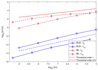
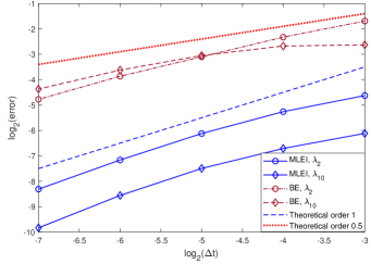
Figure 1. Comparison of BE and MLEI temporal rate of convergence with $f(u)=\sin(u)$ and $\lambda_{2}=4\pi^{2}$, respectively $\lambda_{10}=100\pi^{2}$. Left: with $\rho=1.2$. Right: $\rho=1.75$.

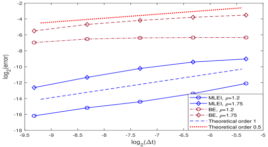
Figure 2. Comparison of BE and MLEI temporal rate of convergence with $f(u)=\sin(u)$, $\rho=1.2$ and $\rho=1.75$ and $\lambda_{30}=900\pi^{2}$.

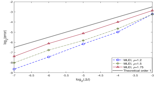
Figure 3. Temporal rate of convergence for MLEI with $f(u)=5(1-u)/(1+u^{2})$, $\rho=1.2,1.5$ and $1.75$ and $\lambda_{2}=4\pi^{2}$.

Figure 4. Solution behaviour with: $f(u)=\sin(u)$, $\rho=1.2$ and $\lambda_{10}=100\pi^{2}$.

Figure 5. Solution behaviour with: $f(u)=\sin(u)$, $\rho=1.75$ and $\lambda_{10}=100\pi^{2}$.

Acknowledgment. We would like thank the anonymous referees for constructive comments that helped us improve the manuscript.

References

• [1] A. Andersson, M Kovács, and S. Larsson, Weak error analysis for semilinear stochastic Volterra equations with additive noise. J. Math. Anal. Appl. 437 (2016), 1283–1304.
• [2] R. Anton, D. Cohen, S. Larsson, and X. Wang, Full discretization of semi-linear stochastic wave equations driven by multiplicative noise. SIAM J. Numer. Anal. 54 (2016), 1093–1119.
• [3] B. Baeumer, M. Geissert, and M. Kovács, Existence, uniqueness and regularity for a class of semilinear stochastic Volterra equations with multiplicative noise. J. Differential Equations 258 (2015), 535–554.
• [4] S. Becker, A. Jentzen, and P. Kloeden, An exponential Wagner-Platen type scheme for SPDES. SIAM J. Numer. Anal. 54 (2016), 2389–2426.
• [5] G. Da Prato and J. Zabczyk, Stochastic Equations in Infinite Dimensions, Encyclopedia Math. Appl., vol. 44, Cambridge University Press, Cambridge, 1992.
• [6] M. Gunzburger, B. Li, and J. Wang, Sharp convergence rates of time discretization for stochastic time-fractional PDEs subject to additive space-time white noise. Math. Comp. 88 (2019), 1715–1741.
• [7] M. Gunzburger, B. Li, and J. Wang, Convergence of finite element solutions of stochastic partial integro-differential equations driven by white noise. Numer. Math. 141 (2019), 1043–1077.
• [8] M. Hochbruck and A. Ostermann, Exponential integrators. Acta Numerica (2010), 209–286.
• [9] A. Jentzen, P. Kloeden, and G. Winkel, Efficient simulation of nonlinear parabolic SPDEs with additive noise. Ann. Appl. Probab. 21 (2011), 908–950.
• [10] M. Kovács, S. Larsson, and F. Lindgren, Weak convergence of finite element approximations of linear stochastic evolution equations with additive noise II: Fully discrete schemes. BIT Numer. Math. 53 (2013), 497–525.
• [11] M. Kovács and J. Printems, Strong order convergence of a fully discrete approximation of a linear stochastic Volterra equation. Math. Comp. 83 (2014), 2325–2346.
• [12] M. Kovács and J. Printems, Weak convergence of a fully discrete approximation of a linear stochastic evolution equation with a positive-type memory term. J. Math. Anal. Appl. 413 (2014), 939–952.
• [13] S. Larsson and M. Molteni, Numerical solution of parabolic problems based on a weak space-time formulation. Comput. Methods Appl. Math. 17 (2017), 65–84.
• [14] G. J. Lord and A. Tambue, Stochastic exponential integrators for the finite element discretization of SPDEs for multiplicative and additive noise. IMA J. Numer. Anal. 33 (2013), 515–543.
• [15] Ch. Lubich, I. Sloan, and V. Thomée, Nonsmooth data error estimates for approximations of an evolution equation with a positive-type memory term. Math. Comp. 65 (1996), 1–17.
• [16] F. Mainardi and P. Paradisi, Fractional diffusive waves. J. Comput. Acoust. 9 (2001), 1417–1436.
• [17] W. McLean and V. Thomée, Numerical solution of an evolution equation with positive memory term. J. Austral. Math. Soc. Ser. B 35 (1993), 23–70.
• [18] I. Podlubny, Fractional Differential Equations, Academic Press, San Diego, 1999.
• [19] I. Podlubny and M. Kacenak, The Matlab mlf code. MATLAB central File Exchange (2001-2009). File ID: 8738.
• [20] J. Prüss, Evolutionary Integral Equations and Applications. Monographs in Mathematics, vol. 87, Birkhäuser, Basel, 1993.
• [21] X. Wang, Strong convergence rates of the linear implicit Euler method for the finite element discretization of SPDEs with additive noise. IMA J. Numer. Anal. 37 (2017), 956–984.
• [22] X. Wang, S. Gan, and J. Tang, Higher order strong approximations of semilinear stochastic wave equation with additive space-time white noise. SIAM J. Sci. Comput. 36 (2014), A2611–A2632.
• [23] X. Wang and R. Qi, A note on an accelerated exponential Euler method for parabolic SPDEs with additive noise. Appl. Math. Letters 46 (2015), 31–37.