Precision neutrino data confronts $\mu\leftrightarrow\tau$ symmetry

Abstract

Neutrino oscillation data indicate that $\theta_{23}$ is close to $\pi/4$ and $\theta_{13}$ is very small. A simple $\mu\leftrightarrow\tau$ exchange symmetry of the neutrino mass matrix predicts $\theta_{23}=-\pi/4$ and $\theta_{13}=0$. Since the experimental measurements differ from these predictions, this symmetry is obviously broken. This breaking is given by two parameters: $\varepsilon_{1}$ parametrizing the inequality bewteen $12$ and $13$ elements and $\varepsilon_{2}$ parametrizing the inequality bewteen $22$ and $33$ elements. We show that the magnitude of $\theta_{13}$ is essentially controlled by $\varepsilon_{1}$ whereas the deviation of $\theta_{23}$ from maximality is controlled by $\varepsilon_{2}$. The measured value of $\theta_{13}$ requires $\mu\leftrightarrow\tau$ symmetry to be badly broken for both normal hierarchy and inverted hierarchy, though the level of breaking depends sensitively on the hierarchy. In this paper we obtain constraints on the parameters of neutrino mass matrix, including the symmetry breaking parameters, using the precision oscillation data. We find that this precision data constrains all elements of neutrino mass matrix to be in very narrow ranges. We also consider $\mu\leftrightarrow-\tau$ exchange symmetry in the case of inverted hierarchy and find that it provides an explanation of neutrino mixing angles with some fine-tuning.

I Introduction

The data from solar Cleveland et al. (1998); Fukuda et al. (1996); Abdurashitov et al. (1994); Hampel et al. (1999); Altmann et al. (2005); Abe et al. (2016); Bahcall et al. (2001) and atmospheric Casper et al. (1991); Nakahata et al. (1986); Ashie et al. (2005) neutrino experiments have provided a strong hint of neutrino oscillations. Later experiments with man made sources measured the neutrino oscillation parameters precisely. These precision measurements lead to stringent constraints on the elements of neutrino mass matrix.

The three flavor states $\nu_{\alpha}$ ($\alpha=e,\mu,\tau$) mix among themselves to form three mass eigenstates $\nu_{i}$ ($i=1,2,3$) which have well-defined mass eigenvalues $m_{1},m_{2}$ and $m_{3}$. The flavor eigenstates are related to the mass eigenstates through the Pontecorvo-Maki-Nakagawa-Sakata (PMNS) mixing matrix $U$ Pontecorvo (1968); Maki et al. (1962) as

$$\nu_{\alpha}=\sum_{i}U_{\alpha i}\nu_{i}.$$ (1)

The elements $U_{\alpha i}$ depend on three mixing angles, $\theta_{12},\theta_{13}$ and $\theta_{23}$ and the CP violating phase ($\delta_{\rm CP}$). From the three mass eigenvalues we can define three mass-squared differences $\Delta m^{2}_{ij}=m^{2}_{i}-m^{2}_{j}$, of which only two are independent. It is known that the mass-squared difference needed to solve the solar neutrino anomaly is much smaller than that to solve the atmospheric neutrino anomaly. Hence we choose $\Delta m^{2}_{21}$ to be the smaller mass-squared difference, which we label as $\delta m^{2}$ and $\Delta m^{2}_{31}$ to be the larger mass-squared difference. The third mass-squared difference, $\Delta m^{2}_{32}=\Delta m^{2}_{31}-\Delta m^{2}_{21}$, is approximately equal to $\Delta m^{2}_{31}$. We define the average of $\Delta m^{2}_{31}$ and $\Delta m^{2}_{32}$ to $\Delta m^{2}$. The neutrino oscillation probabilities depend on the two independent mass-squared differences, $\delta m^{2}$ and $\Delta m^{2}$, the three mixing angles $\theta_{ij}$ and the $\delta_{\rm CP}$ phase.

The expression for the most general three flavor oscillation probability is

$$P(\nu_{\alpha}\to\nu_{\beta}) = \delta_{\alpha\beta}-4\sum_{i>j}{\rm Re}(U^{*}_{\alpha i}U_{\beta i}U_{\alpha j}U^{*}_{\beta j})\sin^{2}\left(1.27\frac{\Delta m^{2}_{ij}L}{E}\right)$$ (2)

$$-2\sum_{i>j}{\rm Im}(U^{*}_{\alpha i}U_{\beta i}U_{\alpha j}U^{*}_{\beta j})\sin\left(2.54\frac{\Delta m^{2}_{ij}L}{E}\right).$$

In principle it is a difficult procedure to determine the oscillation parameters from any experiment given the complicated expression in eq. (2). However two of the parameters in neutrino oscillation formalism are small. CHOOZ experiment set the upper limit $\sin^{2}2\theta_{13}\leq 0.1$, implying that $\theta_{13}$ is small. Solar and atmospheric data show that the ratio $\delta m^{2}/\Delta m^{2}\ll 1$. The smallness of these two quantities enable us to make precision measurements of the mass-squared differences and the mixing angles.

For the long baseline reactor experiment KamLAND Gando et al. (2011), we have $L\sim 180$ km and $E\sim 5$ MeV. For these values we find that $\delta m^{2}L/E\sim 1$ and $\Delta m^{2}L/E\gg 1$. If we substitute $\theta_{13}=0$ in the expression for survival probability of electron anti-neutrinos, we get

$$P(\bar{\nu}_{e}\to\bar{\nu}_{e})=1-\sin^{2}2\theta_{12}\sin^{2}\left(1.27\frac{\delta m^{2}L}{E}\right).$$ (3)

In the approximation of neglecting small $\theta_{13}$, we find that the data of KamLAND experiment can be interpreted in terms of an effective two flavor oscillation formula governed by $\delta m^{2}$ and $\theta_{12}$. The spectral distortion data of KamLAND Araki et al. (2005) leads to a very precise determination of $\delta m^{2}$ and a moderately precise determination of $\tan^{2}\theta_{12}$:

$$\delta m^{2}=7.9^{+0.6}_{-0.5}\times 10^{-5}\ {\rm eV^{2}}\ {\rm and}\ \tan^{2}\theta_{12}=0.4^{+0.10}_{-0.07}.$$ (4)

Solar neutrino data requires $\delta m^{2}$ data to be positive. For long baseline accelerator experiment MINOS Adamson et al. (2013) we have $L\sim 730$ km and $E\sim 3$ GeV. For these values we find that $\delta m^{2}L/E\ll 1$ and $\Delta m^{2}L/E\sim 1$. Hence we set $\delta m^{2}$ and $\theta_{13}$ both equal to zero in the expression for the survival probability of the muon neutrinos. This leads to

$$P(\nu_{\mu}\to\nu_{\mu})=1-\sin^{2}2\theta_{23}\sin^{2}\left(1.27\frac{\Delta m^{2}L}{E}\right).$$ (5)

Once again we have an effective two flavor formula. Analyzing the data of MINOS with this formula leads to precise values of $|\Delta m^{2}|$ and $\sin^{2}2\theta_{23}$:

$$|\Delta m^{2}|=2.41^{+0.09}_{-0.10}\times 10^{-3}\ {\rm eV^{2}}\ {\rm and}\ \sin^{2}2\theta_{23}=0.950^{+0.035}_{-0.036}.$$ (6)

For short baseline reactor experiments Double-CHOOZ Abe et al. (2012), Daya-Bay An et al. (2012) and RENO Ahn et al. (2012) we have $L\sim 1$ km and $E\sim 5$ MeV. If we substitute $\delta m^{2}=0$ in the expression for survival probability of electron anti-neutrinos for these experiments, we again get the effective two flavor expression

$$P(\bar{\nu}_{e}\to\bar{\nu}_{e})=1-\sin^{2}2\theta_{13}\sin^{2}\left(1.27\frac{\Delta m^{2}L}{E}\right).$$ (7)

Using the value of $\Delta m^{2}$ from MINOS experiment, the value $\sin^{2}\theta_{13}$ is measured to be Huang (2016)

$$\sin^{2}2\theta_{13}=0.0841\pm 0.0027{\rm(stat.)}\pm 0.0019{\rm(syst.)}.$$ (8)

In Table 1 we have shown the results of the global analysis of all neutrino oscillation data, including solar, atmospheric, reactor and accelerator sources Esteban et al. (2017).

Parameter	Best Fit	1$\sigma\ {\rm range}$	3$\sigma\ {\rm range}$
$\delta m^{2}/10^{-5}{\rm\ eV^{2}\ (NH\ or\ IH)}$	7.50	7.33 - 7.69	7.03 - 8.09
$\sin^{2}\theta_{12}{\rm\ (NH\ or\ IH)}$	0.306	0.294 - 0.318	0.271 - 0.345
$\Delta m^{2}/10^{-3}{\rm\ eV^{2}\ (NH)}$	2.524	2.484 - 2.563	2.407 - 2.643
$\Delta m^{2}/10^{-3}{\rm\ eV^{2}\ (IH)}$	-2.514	-2.555 - -2.476	-2.635 - -2.399
$\sin^{2}\theta_{13}{\rm\ (NH)}$	0.02166	0.02091 - 0.02241	0.01934 - 0.02392
$\sin^{2}\theta_{13}{\rm\ (IH)}$	0.02179	0.02103 - 0.02255	0.01953 - 0.02408
$\sin^{2}\theta_{23}{\rm\ (NH)}$	0.441	0.420 - 0.468	0.385 - 0.635
$\sin^{2}\theta_{23}{\rm\ (IH)}$	0.587	0.563 - 0.607	0.393 - 0.640

Table 1: Global Data of three neutrino mass-mixing parameters Esteban et al. (2017)

From this data, we note the following features:

• Neutrino oscillation data does not give any information on the lowest value of neutrino mass. It can be almost zero or be equal to the upper limit from Tritium beta decay of $0.2$ eV Kraus et al. (2005).

• Since the sign of $\Delta m^{2}_{31}$ is not known, we need to consider both possible signs. For $\Delta m^{2}_{31}$ positive, called the normal hierarchy (NH), the lowest mass is $m_{1}$ and the highest mass is $m_{3}$. For $\Delta m^{2}_{31}$ negative, called the inverted hierarchy (IH), the lowest mass is $m_{3}$ and the highest mass is $m_{2}$.

• The neutrino mass eigenstates $\nu_{i}$ ($i=1,2,3$) are identified by their $\nu_{e}$ flavor content, which is largest for $\nu_{1}$ and smallest for $\nu_{3}$.

• Among the mixing angles, $\theta_{23}$ is close to maximal and $\theta_{13}$ is quite small.

Various discrete symmetries of the neutrino mass matrix have been proposed to account for the patterns observed in neutrino masses and mixing angles. The simplest of these is the $\mu\leftrightarrow\tau$ exchange symmetry of neutrino mass matrix Harrison and Scott (2002). This symmetry predicts $\theta_{23}=-\pi/4$ and $\theta_{13}=0$. In this paper, we will study

• the pattern of $\mu\leftrightarrow\tau$ symmetry breaking to obtain viable values of $\theta_{13}$ and $\theta_{23}$ and

• the constraints imposed on the parameters of neutrino mass matrix by the precision oscillation data.

II $\mu\leftrightarrow\tau$ Symmetry

We assume neutrinos are Majorana fermions and the light neutrino mass matrix is generated through a see-saw mechanism. The Majorana mass matrix for light neutrinos is a complex symmetric matrix. In this work we assume it to be real, which (a) simplifies the discussion and (b) makes the analysis more predictive:

$$M_{0}=\left(\begin{array}[]{ccc}M_{ee}&M_{e\mu}&M_{e\tau}\\ M_{e\mu}&M_{\mu\mu}&M_{\mu\tau}\\ M_{e\tau}&M_{\mu\tau}&M_{\tau\tau}\end{array}\right)=\left(\begin{array}[]{ccc}a&b_{1}&b_{2}\\ b_{1}&c_{1}&d\\ b_{2}&d&c_{2}\end{array}\right).$$ (9)

Imposing the $\mu\leftrightarrow\tau$ symmetry Fukuyama and Nishiura (1997); Ma and Raidal (2001); Lam (2001); Xing and Zhao (2016) on this mass matrix leads to $b_{1}=b_{2}=b$ and $c_{1}=c_{2}=c$. This real symmetric matrix is diagonalized by the orthogonal matrix,

$$\left(\begin{array}[]{ccc}\cos\theta_{12}&\sin\theta_{12}&0\\ -\frac{1}{\sqrt{2}}\sin\theta_{12}&\frac{1}{\sqrt{2}}\cos\theta_{12}&-\frac{1}{\sqrt{2}}\\ -\frac{1}{\sqrt{2}}\sin\theta_{12}&\frac{1}{\sqrt{2}}\cos\theta_{12}&\frac{1}{\sqrt{2}}\end{array}\right).$$ (10)

By inspection we can identify $\theta_{13}=0$ and $\theta_{23}=-\pi/4$ and the value of $\theta_{12}$ is given by

$$\tan 2\theta_{12}=\frac{2\sqrt{2}b}{c+d-a}.$$ (11)

The mass eigenvalues are given by

$$m_{1} = \frac{a+c+d-k}{2}$$

$$m_{2} = \frac{a+c+d+k}{2}$$

$$m_{3} = c-d,$$ (12)

where $k=\sqrt{(c+d-a)^{2}+8b^{2}}$. The measured value of $\theta_{12}$ leads to $\sin^{2}\theta_{12}\approx 1/3$. Substituting it in the above equation leads to the two relations

$$b=c+d-a\ {\rm and}\ k=3b.$$ (13)

The expressions for the mass-squared differences are obtained to be

$$\delta m^{2} = m^{2}_{2}-m^{2}_{1}$$ (14)

$$= k(a+c+d)$$

and

$$\Delta m^{2} = m^{2}_{3}-\frac{m^{2}_{1}+m^{2}_{2}}{2}$$ (15)

$$= \frac{1}{2}\left[(c-d)^{2}-4cd-a^{2}-4b^{2}\right].$$

Since only the magnitude of $\Delta m^{2}$ is measured there is a sign ambiguity in the constraint of eq. (15). All the four parameters of the neutrino mass matrix can be exactly determined provided (a) this sign ambiguity is resolved and (b) the lowest mass eigenvalue is known. In the following, we take the lowest mass eigenvalue to be negligibly small. With this assumption, we will work out the values for neutrino mass eigenvalues and the neutrino mass matrix parameters for the two cases of normal hierarchy (NH, $m_{3}>m_{2}\gg m_{1}$) and inverted hierarchy (IH, $m_{2}\geq m_{1}\gg m_{3}$).

II.1 Normal Hierarchy

For normal hierarchy, $\Delta m^{2}$ is positive and we choose $m_{1}$ to be negligibly small. This assumption leads

$$a+c+d\approx k=3b\ {\rm and}\ \delta m^{2}\approx k^{2},$$ (16)

yielding

$$b=\frac{k}{3}\approx\frac{\sqrt{\delta m^{2}}}{3}.$$ (17)

Combining with the condition from eq. (13), we get

$$a\approx b\ {\rm and}\ c+d\approx 2b.$$ (18)

From the expression of $\Delta m^{2}$ in eq. (15), we note that

$$\Delta m^{2}\approx\frac{1}{2}[(c-d)^{2}-4cd],$$ (19)

which is satisfied if

$$c\approx-d\approx\frac{\sqrt{\Delta m^{2}}}{2}\gg a,b.$$ (20)

From eqs. (11) and (20), we see that the large value of $\theta_{12}$ arises due to a fine-tuned cancellation in $(c+d-a)$, which makes its value equal to $b$. From eqs. (17) and (20), we see that this cancellation is of the order $\sqrt{\delta m^{2}/\Delta m^{2}}$. Thus the four parameters of the neutrino mass matrix are determined exactly by the four conditions, given by the three measured parameters $\sin^{2}\theta_{12}$, $\delta m^{2}$ and $\Delta m^{2}$ and the assumption on the lowest mass eigenvalue.

We impose the less rigid constraint that the measured values should be within their $3\sigma$ ranges, as given below

$$0.271\leq\sin^{2}\theta_{12}\leq 0.345$$

$$7.03\times 10^{-5}\leq\delta m^{2}\leq 8.09\times 10^{-5}$$

$$2.407\times 10^{-3}\leq\Delta m^{2}\leq 2.643\times 10^{-3}$$

$$|m_{1}|<0.1\ m_{2}.$$ (21)

The allowed ranges of the $a,b,c$ and $d$ are

$$a = 0.0017-0.0036$$

$$b = 0.0025-0.0031$$

$$c = 0.027-0.028$$

$$d = -0.022--0.021.$$ (22)

The values in eq. (II.1) satisfy the constraints mentioned in eq. (20).

II.2 Inverted Hierarchy

For inverted hierarchy, $\Delta m^{2}$ is negative and we choose $m_{3}$ to be negligibly small leading to $c\approx d$. The ratio of the two mass-squared differences is

$$\frac{\delta m^{2}}{|\Delta m^{2}|}=\frac{6b(2c+a)}{4c^{2}+a^{2}+4b^{2}}=0.03.$$ (23)

This equation is satisfied if

$$a\approx 2c\ {\rm and}\ \frac{b}{c}\approx 0.01.$$ (24)

The constraint from eq. (11) forbids the other possibility $b\gg a,c,d$. From eq. (24), we see that the value of $(c+d-a)$ should be fine-tuned to $0.5\%$ [$\sim 0.1(\delta m^{2}/\Delta m^{2}$)] to obtain the correct value of $\theta_{12}$. This is a much more delicate fine-tuning compared to the NH case.

Demanding that the measured parameters should be within their $3\sigma$ ranges we get the inequalities

$$0.271\leq\sin^{2}\theta_{12}\leq 0.345$$

$$7.03\times 10^{-5}\leq\delta m^{2}\leq 8.09\times 10^{-5}$$

$$-2.635\times 10^{-3}\leq\Delta m^{2}\leq-2.399\times 10^{-3}$$

$$|m_{3}|<0.1\ m_{1}.$$ (25)

This leads to the allowed ranges for $a,b,c$ and $d$

$$a = 0.0466-0.0506$$

$$b = 0.00024-0.00027$$

$$c = 0.0216-0.0278$$

$$d = 0.0214-0.0278,$$ (26)

which satisfy the constraints mentioned above. In the case of NH, $b\sim\sqrt{\delta m^{2}}$ whereas in the case of IH, $b\sim\delta m^{2}/a$. Therefore, the value of $b$ in case of IH is an order of magnitude smaller than in the case of NH, whereas the value $a$ is an order of magnitude larger than in the case of NH. Note that the magnitudes of $c$ and $d$ are the same in both cases.

III $\mu\leftrightarrow\tau$ symmetry breaking through ’$\varepsilon_{1}$’

$\mu\leftrightarrow\tau$ symmetry involves two conditions $b_{1}=b_{2}$ and $c_{1}=c_{2}$, as seen from eq. (9). A violation of either of these conditions leads to a breaking of $\mu\leftrightarrow\tau$ symmetry. We first consider the breaking of the condition $b_{1}=b_{2}$. We parametrize this breaking as $b_{1}=b-\varepsilon_{1}$ and $b_{2}=b+\varepsilon_{1}$, leading to the neutrino mass matrix,

$$M_{1}=\left(\begin{array}[]{ccc}a&b-\varepsilon_{1}&b+\varepsilon_{1}\\ b-\varepsilon_{1}&c&d\\ b+\varepsilon_{1}&d&c\end{array}\right).$$ (27)

Since $\varepsilon_{1}$ breaks $\mu\leftrightarrow\tau$ exchange symmetry, the values of $\theta_{13}$ and $\theta_{23}$ predicted by the mass matrix in eq. (27) will differ from $0$ and $\pi/4$ respectively. The characteristic equation for the perturbed mass matrix is

$$\lambda^{3}-\lambda^{2}(2c+a)+\lambda(2ca+c^{2}-d^{2}-2b^{2}-2\varepsilon_{1}^{2})-[a(c^{2}-d^{2})+2b^{2}(c+d)+2\varepsilon_{1}^{2}(c-d)]=0.$$ (28)

If we impose the condition that the lowest mass eigenvalue is negligibly small, the quantity in the square brackets in the above equation should be close to zero. For both NH and IH, we have $c^{2}\approx d^{2}$ and $b\ll c,d$. Hence the first two terms are negligibly small. We require $\varepsilon_{1}$ to be much less than $c,d$ to satisfy the constraint on the lowest mass eigenvalue. In this approximation, the characteristic equation simplifies to

$$\lambda[\lambda^{2}-\lambda(2c+a)+2ca]=0,$$ (29)

whose eigenvalues are $0$, $a$, $2c$. We discuss the cases of NH and IH separately.

III.1 Normal Hierarchy

For NH, we have $a\approx\sqrt{\delta m^{2}}$ and $c\approx\sqrt{\Delta m^{2}}/2$. The first element of the eigenvector corresponding to the eigenvalue $m_{3}$ gives us $\sin\theta_{13}$. For NH, $m_{3}\approx 2c$, and the corresponding eigenvector is

$$|\nu_{3}\rangle\approx\left[\begin{array}[]{c}\frac{\sqrt{2}\varepsilon_{1}}{(2c-a)}\\ -\frac{1}{\sqrt{2}}\\ \frac{1}{\sqrt{2}}\end{array}\right].$$ (30)

The value of $\sin^{2}\theta_{13}$ can be approximated as $\varepsilon_{1}^{2}/(2c^{2})$ because $c\gg a$. To obtain $\sin^{2}\theta_{13}\simeq 0.02$, we must have $\varepsilon_{1}\geq b$. Hence we see from eq. (27) that $\varepsilon_{1}$ can not be treated as a perturbation of the $\mu\leftrightarrow\tau$ symmetric matrix.

We now do a numerical calculation to find the ranges of $a,b,c,d$ and $\varepsilon_{1}$ allowed by the neutrino oscillation data. We find the eigenvalues of matrix in eq. (27) and label them as $m_{1},m_{2}$ and $m_{3}$ in increasing order. The diagonalizing matrix is parametrized as

$$U=\left(\begin{array}[]{ccc}U_{e1}&U_{e2}&U_{e3}\\ U_{\mu 1}&U_{\mu 2}&U_{\mu 3}\\ U_{\tau 1}&U_{\tau 2}&U_{\tau 3}\end{array}\right).$$ (31)

The 5 oscillation parameters are defined as:

$$\delta m^{2} = m^{2}_{2}-m^{2}_{1},$$

$$\Delta m^{2} = m^{2}_{3}-\frac{m^{2}_{1}+m^{2}_{2}}{2},$$

$$\sin^{2}\theta_{13} = U^{2}_{e3},$$

$$\sin^{2}\theta_{23} = \frac{U^{2}_{\mu 3}}{1-U^{2}_{e3}},$$

$$\sin^{2}\theta_{12} = \frac{U^{2}_{e2}}{1-U^{2}_{e3}}.$$ (32)

As we saw above, the value of $\varepsilon_{1}$ needed to generate the correct magnitude of $\theta_{13}$ means $\varepsilon_{1}\geq b$. Therefore, we treat $\varepsilon_{1}$ as a free parameter and numerically search for allowed values of $a,b,c,d$ and $\varepsilon_{1}$ which satisfy the following $3\sigma$ experimental constraints on $\sin^{2}\theta_{13}$ and $\sin^{2}\theta_{23}$

$$0.385\leq\sin^{2}\theta_{23}\leq 0.635$$

$$0.01934\leq\sin^{2}\theta_{13}\leq 0.02392,$$ (33)

in addition to the four constraints already given in eq. (II.1). Our numerical search gives

$$a = 0.0027-0.0046$$

$$b = 0.0026-0.0032$$

$$c = 0.028$$

$$d = -0.022$$

$$\varepsilon_{1} = -0.0053--0.0046.$$ (34)

For the central value $\varepsilon_{1}=-0.0050$, we get $\sin^{2}\theta_{12}=0.298$, $\sin^{2}\theta_{13}=0.0221$ and $\sin^{2}\theta_{23}=0.514$. The T2K experiment observes maximal $\nu_{\mu}$ disappearance, implying $|U_{\mu 3}|^{2}=0.5=\cos^{2}\theta_{13}\sin^{2}\theta_{23}$. On substituting the reactor measurements of $\theta_{13}$, this leads to $\sin^{2}\theta_{23}=0.514$, which is equal to the prediction above. It is interesting to note that the value of $\varepsilon_{1}$, needed to produce the correct value of $\sin^{2}\theta_{13}$ also produces the correct deviation in $\sin^{2}\theta_{23}$ needed to explain the T2K $\nu_{\mu}$ disappearance data. The variation of $sin^{2}\theta_{ij}$ vs. $\varepsilon_{1}$ is plotted in fig. 1, for NH. It was mentioned earlier that a fine-tuning of neutrino mass matrix parameters is required to obtain viable values of $\theta_{12}$. There is a significant variation of $\sin^{2}\theta_{12}$ with respect to $\varepsilon_{1}$ because of this fine-tuning. As shown above, $\sin^{2}\theta_{13}$ varies as $\varepsilon_{1}^{2}$. We see that $\sin^{2}\theta_{23}$ shows a small linear variation with respect to $\varepsilon_{1}$.

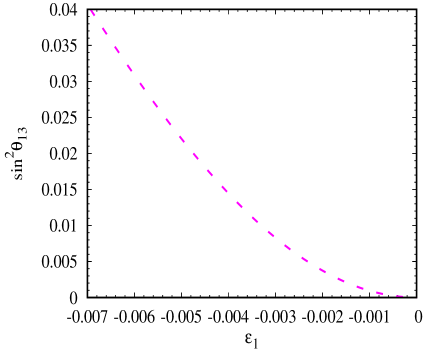
(a)   (b) (c)

Figure 1: Plots of $\sin^{2}\theta_{ij}$ vs. $\varepsilon_{1}$ for the central values of NH neutrino mass matrix elements.

III.2 Inverted Hierarchy

For IH, $m_{3}\approx 0$, whose eigenvector is

$$|\nu_{3}\rangle\approx\left[\begin{array}[]{c}-\frac{\sqrt{2}\varepsilon_{1}}{a}\\ -\frac{1}{\sqrt{2}}\\ \frac{1}{\sqrt{2}}\end{array}\right].$$ (35)

Hence $\sin^{2}\theta_{13}=2\varepsilon_{1}^{2}/a^{2}$. Since the value of $a$ in IH is the same as the value of $2c$ in NH ($\approx\sqrt{\Delta m^{2}}$), the magnitude of $\varepsilon_{1}$ in this case is of a similar magnitude as that of NH. But the value of $b$ in IH is an order of magnitude lower than the case of NH and hence we have $b\ll\varepsilon_{1}$ in the case of IH. Here $\varepsilon_{1}$ most definitely can not be treated as a perturbation on $b$.

For IH, the lowest eigenvalue of the matrix in eq. (27) is labeled $m_{3}$, the middle one is labeled $m_{1}$ and the highest $m_{2}$. The diagonalizing matrix is labeled as in eq. (31) and the definitions of the five oscillation parameters remain the same as those in eq. (III.1). For this case also we do a numerical search to find ranges of $a,b,c,d$ and $\varepsilon_{1}$ which satisfy the six experimental constraints given in eqs. (II.2) and (III.1). The search yields the ranges

$$a = 0.048-0.050$$

$$b = 0.00022-0.00027$$

$$c = 0.023-0.026$$

$$d = 0.0243-0.0277$$

$$\varepsilon_{1} = -0.0061--0.0049.$$ (36)

For the central value $\varepsilon_{1}=-0.0052$, we get $\sin^{2}\theta_{12}=0.306$, $\sin^{2}\theta_{13}=0.0223$ and $\sin^{2}\theta_{23}=0.501$. The variation of $sin^{2}\theta_{ij}$ vs. $\varepsilon_{1}$ is plotted in fig. 2, for IH. Since $b$ is too small, extreme fine-tuning is needed to obtain the appropriate value of $\sin^{2}\theta_{12}$. The variation of $\sin^{2}\theta_{12}$, with respect to $\varepsilon_{1}$, is very pronounced because of this extreme fine-tuning. As in the case of NH, $\sin^{2}\theta_{13}$ varies as $\varepsilon_{1}^{2}$ and $\sin^{2}\theta_{23}$ shows a small linear variation with respect to $\varepsilon_{1}$.

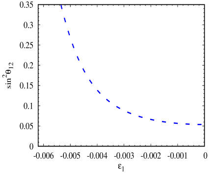
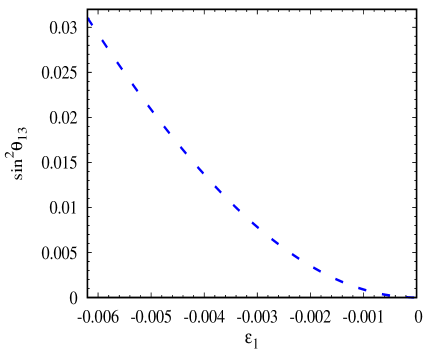
(a)   (b) (c)

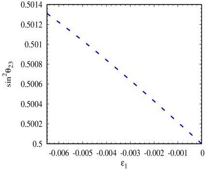
Figure 2: Plots of $\sin^{2}\theta_{ij}$ vs. $\varepsilon_{1}$ for the central values of IH neutrino mass matrix elements.

IV $\mu\leftrightarrow\tau$ symmetry breaking through ’$\varepsilon_{2}$’

Now we hold the equality $b_{1}=b_{2}=b$ in eq. (9) but assume $c_{1}\neq c_{2}$. We parametrize this breaking of $\mu\leftrightarrow\tau$ symmetry as $c_{1}=c-\varepsilon_{2}$ and $c_{2}=c+\varepsilon_{2}$. The neutrino mass matrix has the form

$$M_{2}=\left(\begin{array}[]{ccc}a&b&b\\ b&c-\varepsilon_{2}&d\\ b&d&c+\varepsilon_{2}\end{array}\right).$$ (37)

The $2-3$ block is diagonalized by applying the similarity transformation $U_{23}^{T}M_{2}U_{23}$, where

$$U_{23}=\left(\begin{array}[]{ccc}1&0&0\\ 0&\cos\theta_{23}&\sin\theta_{23}\\ 0&-\sin\theta_{23}&\cos\theta_{23}\end{array}\right).$$ (38)

In the above equation $\theta_{23}\neq-\pi/4$ but is taken to be $-\pi/4+\delta\theta_{23}$. The deviation from maximality is found to be

$$\delta\theta_{23}\simeq-\frac{\varepsilon_{2}}{2d}.$$ (39)

From neutrino data in Table 1, the maximum allowed value of this quantity is $0.12$ Esteban et al. (2017). The $13$ element of the rotated mass matrix is $\sqrt{2}b\varepsilon_{2}/(2d)$. This term determines the value of $\sin\theta_{13}$. (The corresponding quantity in the case of $\varepsilon_{1}$ symmetry breaking is $\sqrt{2}\varepsilon_{1}$). Given the limit on $\delta\theta_{23}$, we find $b\varepsilon_{2}/(\sqrt{2}d)$ is an order of magnitude smaller than $b$.

In the earlier discussion on $\varepsilon_{1}$ symmetry breaking, it was shown that $\varepsilon_{1}\simeq 0.005$ to reproduce the correct $\sin^{2}\theta_{13}$. Therefore the term generating non-zero $\theta_{13}$ for $\varepsilon_{2}$ symmetry breaking is an order of magnitude lower for NH ($b\sim 0.002$) and two orders of magnitude lower for IH ($b\sim 0.0002$). Hence it is impossible to satisfy the constraints on $\sin^{2}\theta_{13}$ and $\sin^{2}\theta_{23}$ only through $\varepsilon_{2}$ breaking. The maximum allowed values of $\sin^{2}\theta_{13}$ we get in this case are of the order of $10^{-5}$ for NH and $10^{-7}$ for IH.

V Complete $\mu\leftrightarrow\tau$ Symmetry Breaking

In the above sections, we saw that $\varepsilon_{1}$ symmetry breaking generates acceptable value of $\sin^{2}\theta_{13}$ but keeps the value of $\sin^{2}\theta_{23}$ close to maximal. On the other hand, $\varepsilon_{2}$ symmetry breaking leads to significant deviation of $\sin^{2}\theta_{23}$ away from maximality but predicts very small values for $\sin^{2}\theta_{13}$. If later data confirms that $\sin^{2}\theta_{23}$ is non-maximal, we need to introduce both $\varepsilon_{1}$ and $\varepsilon_{2}$ symmetry breaking to describe the neutrino mixing angles accurately. In such a situation, the value of $\varepsilon_{1}$ is essentially determined by $\sin^{2}\theta_{13}$ and that of $\varepsilon_{2}$ is determined by the deviation of $\theta_{23}$ from maximality.

The neutrino mass matrix is described by six parameters: $a,b,c,d,\varepsilon_{1}$ and $\varepsilon_{2}$. We search for the allowed values of these parameters by demanding that the two mass-squared differences and the three mixing angles should be within their allowed $3\sigma$ ranges. We also impose a sixth constraint that lowest neutrino mass ($m_{1}$ for NH and $m_{3}$ for IH) should be less than $0.001$ eV. With these constraints we obtain the following allowed ranges of parameters. For NH

$$a = 0.0027-0.0046$$ (40)

$$|b| = 0.0026-0.0038$$

$$c = 0.028$$

$$d = -0.022$$

$$|\varepsilon_{1}| = 0.0043-0.0052$$

$$|\varepsilon_{2}| = 0.0-0.0046.$$

Similarly for IH,

$$a = 0.0048-0.0050$$ (41)

$$|b| = 0.0-0.00027$$

$$c = 0.023-0.028$$

$$d = 0.0210-0.0270$$

$$|\varepsilon_{1}| = 0.0044-0.0058$$

$$|\varepsilon_{2}| = 0.0-0.0026.$$

Earlier we saw the following patterns: for NH $d\approx-c$, $a\approx b\approx\varepsilon_{1}$ and for IH $c\approx d\approx a/2$, $b\ll\varepsilon_{1}$ with $\varepsilon_{1}\rm{(NH)}=\varepsilon_{1}\rm{(IH)}$. From above equations we see that the same relations hold here also.

VI Ranges of neutrino mass matrix parameters from precision oscillation data

In the previous sections we varied the parameters of neutrino mass matrix to find their values which satisfy the experimental constraints. As we can see from eqs. (40) and (41), the ranges for these parameters are quite small. In this section, we do a systematic search to find the exact ranges of these parameters allowed by the current oscillation data. Among the oscillation observables, the mass-squared differences, $\delta m^{2}$ Gando et al. (2011)and $|\Delta m^{2}|$ Adamson et al. (2013); Abe et al. (2011); Adamson et al. (2017), are measured to better than $3\%$ precision. The mixing angles, $\sin^{2}\theta_{12}$ Abdurashitov et al. (1994); Hampel et al. (1999); Abe et al. (2016); Ahmad et al. (2001); Bahcall et al. (2001) and $\sin^{2}\theta_{13}$ An et al. (2012), are determined to about $4\%$ precision. The precision in $\sin^{2}\theta_{23}$ is poorer because of the octant ambiguity Adamson et al. (2013); Abe et al. (2011); Adamson et al. (2017). Below we study the impact of these precision measurements on the allowed ranges of neutrino mass parameters.

We use the following procedure. We first choose a value for the lowest neutrino mass eigenvalue. We then choose five uniform random numbers in the interval [-1,1]. Using these numbers, we construct random values for the five neutrino oscillation parameters within their $1\ \sigma$ ranges. We construct the diagonal neutrino mass matrix using the lowest neutrino mass and the two mass-squared differences. For NH, the diagonal form of the mass matrix is

$$M_{\rm diag}=\left(\begin{array}[]{ccc}m_{1}&&\\ &\sqrt{m_{1}^{2}+\delta m^{2}}&\\ &&\sqrt{m_{1}^{2}+\delta m^{2}/2+\Delta m^{2}}\end{array}\right),$$ (42)

where $m_{1}$ is the lowest neutrino mass chosen, whereas for IH, this matrix takes the form

$$M_{\rm diag}=\left(\begin{array}[]{ccc}\sqrt{m_{3}^{2}-\delta m^{2}/2+|\Delta m^{2}|}&&\\ &\sqrt{m_{3}^{2}+\delta m^{2}/2+|\Delta m^{2}|}&\\ &&m_{3}\end{array}\right),$$ (43)

where $m_{3}$ is the lowest neutrino mass. We obtain the neutrino mass matrix in flavor basis by the similarity transformation $M_{0}=UM_{\rm diag}U^{T}$, where $U$ is the orthogonal matrix constructed using the values of the three chosen mixing angles.

For a given set of five random numbers we get the corresponding set of neutrino oscillation parameters which in turn lead to a given set of values for $a,b,c,d,\varepsilon_{1}$ and $\varepsilon_{2}$. We repeat this procedure for 10,000 sets of five random numbers to produce 10,000 values of neutrino mass matrix parameters. From these 10,000 sets of parameter values we tabulate the mean, the standard deviation, the lowest and the highest values. This procedure is used to construct the allowed ranges of neutrino mass matrix elements for the following eight cases: for NH, $m_{1}=0,0.001,0.01$ and $0.1$ eV and for IH, $m_{3}=0,0.001,0.01$ and $0.1$ eV.

From these tables we note the following patterns. The ranges for the neutrino mass matrix elements, whose magnitudes are large, are $\lesssim 1\%$. This is true for the parameters $c$ and $d$ in all cases and for the parameter $a$ in the case of IH and when the minimum neutrino mass $m_{1}\geq 0.01$ eV in the case of NH. Since $\sin^{2}\theta_{13}\propto\varepsilon_{1}^{2}$, the range of $\varepsilon_{1}$ is about $2\%$, which is half the uncertainty in $\sin^{2}\theta_{13}$. The range of $\varepsilon_{2}$ is about $10\%$ in case of NH and about $25\%$ in case of IH. The values and ranges of $b$ are usually very small because of the need to otain the correct value of $\theta_{12}$.

Matrix	Lower	Upper	Mean	Standard
Element	Bound	Bound		Deviation
$a$	0.005426	0.006546	0.005971	0.0002192
$b$	-0.001934	-0.001568	-0.001752	0.00007519
$c$	0.02621	0.02708	0.02665	0.0001534
$d$	-0.02007	-0.01941	-0.01974	0.0001215
$\varepsilon_{1}$	0.008661	0.009855	0.009252	0.0002200
$\varepsilon_{2}$	0.003840	0.005704	0.004773	0.0004379

Table 2: Normal Hierarchy: $m_{1}=0.0$ eV

Matrix	Lower	Upper	Mean	Standard
Element	Bound	Bound		Deviation
$a$	0.006123	0.007233	0.006665	0.0002130
$b$	-0.001684	-0.001298	-0.001484	0.00007498
$c$	0.02639	0.02729	0.02684	0.0001495
$d$	-0.01996	-0.01932	-0.01964	0.0001208
$\varepsilon_{1}$	0.008506	0.009695	0.009089	0.0002174
$\varepsilon_{2}$	0.003708	0.005507	0.004630	0.0004337

Table 3: Normal Hierarchy: $m_{1}=0.001$ eV

Matrix	Lower	Upper	Mean	Standard
Element	Bound	Bound		Deviation
$a$	0.01352	0.01443	0.01395	0.0001761
$b$	-0.0004328	-0.00008957	-0.0002615	0.00006912
$c$	0.03005	0.03082	0.03043	0.0001347
$d$	-0.01797	-0.01738	-0.01768	0.0001167
$\varepsilon_{1}$	0.007172	0.008227	0.007688	0.0001947
$\varepsilon_{2}$	0.002904	0.004506	0.003707	0.0003989

Table 4: Normal Hierarchy: $m_{1}=0.01$ eV

Matrix	Lower	Upper	Mean	Standard
Element	Bound	Bound		Deviation
$a$	0.1009	0.1012	0.1010	0.00005170
$b$	0.00004479	0.0001452	0.00009461	0.00002089
$c$	0.1056	0.1059	0.1057	0.00005338
$d$	-0.005459	-0.005226	-0.005343	0.00004978
$\varepsilon_{1}$	0.002074	0.002424	0.002245	0.00006093
$\varepsilon_{2}$	0.0007954	0.001298	0.001044	0.0001206

Table 5: Normal Hierarchy: $m_{1}=0.1$ eV

Matrix	Lower	Upper	Mean	Standard
Element	Bound	Bound		Deviation
$a$	0.04318	0.04504	0.04413	0.0003216
$b$	$4.258\times 10^{-6}$	0.0005179	0.0002587	0.0001321
$c$	0.02810	0.02909	0.02859	0.0001770
$d$	0.02114	0.02218	0.02168	0.0001833
$\varepsilon_{1}$	-0.01176	-0.01062	-0.01120	0.0002125
$\varepsilon_{2}$	0.0009376	0.002888	0.001915	0.0004803

Table 6: Inverted Hierarchy: $m_{3}=0.0$ eV

Matrix	Lower	Upper	Mean	Standard
Element	Bound	Bound		Deviation
$a$	0.04319	0.04501	0.04412	0.0003206
$b$	$-6.945\times 10^{-7}$	0.0005158	0.0002593	0.0001309
$c$	0.02809	0.02912	0.02859	0.0001793
$d$	0.02115	0.02217	0.02167	0.0001826
$\varepsilon_{1}$	-0.01179	-0.01061	-0.01120	0.0002152
$\varepsilon_{2}$	0.0009429	0.002899	0.001917	0.0004754

Table 7: Inverted Hierarchy: $m_{3}=0.001$ eV

Matrix	Lower	Upper	Mean	Standard
Element	Bound	Bound		Deviation
$a$	0.04526	0.04685	0.04606	0.0002858
$b$	-0.00003361	0.0004061	0.0001856	0.0001106
$c$	0.03264	0.03355	0.03310	0.0001632
$d$	0.01770	0.01859	0.01815	0.0001604
$\varepsilon_{1}$	-0.009867	-0.008859	-0.009364	0.0001802
$\varepsilon_{2}$	0.0007994	0.002452	0.001618	0.0004015

Table 8: Inverted Hierarchy: $m_{3}=0.01$ eV

Matrix	Lower	Upper	Mean	Standard
Element	Bound	Bound		Deviation
$a$	0.1101	0.1107	0.1104	0.0001094
$b$	-0.00004422	0.00008396	0.00001912	0.00003190
$c$	0.1065	0.1068	0.1067	0.00006381
$d$	0.005095	0.005409	0.005255	0.00005902
$\varepsilon_{1}$	-0.002854	-0.002540	-0.002696	0.00005532
$\varepsilon_{2}$	0.0002519	0.0007285	0.0004873	0.0001155

Table 9: Inverted Hierarchy: $m_{3}=0.1$ eV

VII $\mu\leftrightarrow-\tau$ symmetry

From the tables given in the previous section, we note that $b=0$ is an accepted value for the case of IH. In this section, we explore the allowed values of neutrino mass matrix with the constraint $b\equiv 0$. It is possible to impose such a constraint through $\mu\leftrightarrow-\tau$ exchange symmetry. Under this symmetry, the $\varepsilon_{1}$ term is naturally non-zero.

The most general neutrino mass matrix invariant under this symmetry is

$$M_{3}=\left(\begin{array}[]{ccc}a&-\varepsilon_{1}&\varepsilon_{1}\\ -\varepsilon_{1}&c&d\\ \varepsilon_{1}&d&c\end{array}\right).$$ (44)

Diagonalizing this matrix, we find $\theta_{23}=-\pi/4$, $\theta_{12}=0$ and

$$\tan 2\theta_{13}=\frac{2\sqrt{2}\varepsilon_{1}}{c-d-a}\approx-\frac{2\sqrt{2}\varepsilon_{1}}{a},$$ (45)

because $c\approx d$ for IH. Also, we note that $a\approx 2c$. This, except for $\theta_{23}$, is exactly opposite to $\mu\leftrightarrow\tau$ symmetry case where we had $\theta_{13}=0$ and $\tan 2\theta_{12}=2\sqrt{2}b/(c+d-a)$. Since $\theta_{13}\ll 1$, the above equation implies that $\varepsilon_{1}\ll a,c,d$. Obviously, $\mu\leftrightarrow-\tau$ is not exact because it predicts $\theta_{12}=0$. It can be broken through $\varepsilon_{2}$ term introduced in $22$ and $33$ elements as in the case of $\mu\leftrightarrow\tau$ symmetry. We will show below that such a breaking can lead to both non-maximal $\theta_{23}$ as well as viable values of $\theta_{12}$. However to obtain $\theta_{12}$ within the experimentally allowed range, we need to fine-tune the combination $c+d-a$ to order $\varepsilon_{1}^{2}/a$.

With the $\varepsilon_{2}$ symmetry breaking the neutrino mass matrix becomes

$$M_{4}=\left(\begin{array}[]{ccc}a&-\varepsilon_{1}&\varepsilon_{1}\\ -\varepsilon_{1}&c-\varepsilon_{2}&d\\ \varepsilon_{1}&d&c+\varepsilon_{2}\end{array}\right).$$ (46)

Applying the similarity transformation $U_{23}^{T}M_{4}U_{23}$, where $U_{23}$ is defined in eq. (38), we get

$$U^{T}_{23}M_{4}U_{23}=\left(\begin{array}[]{ccc}a&-\sqrt{2}\varepsilon_{1}\sin\delta\theta_{23}&\sqrt{2}\varepsilon_{1}\cos\delta\theta_{23}\\ -\sqrt{2}\varepsilon_{1}\sin\delta\theta_{23}&c+d\sqrt{1+\frac{\varepsilon_{2}^{2}}{d^{2}}}&0\\ \sqrt{2}\varepsilon_{1}\cos\delta\theta_{23}&0&c-d\sqrt{1+\frac{\varepsilon_{2}^{2}}{d^{2}}}\end{array}\right).$$ (47)

Here, $\delta\theta_{23}$ is the deviation of $\theta_{23}$ from maximality and it is given by $\tan 2\delta\theta_{23}=-\varepsilon_{2}/d$. Note that the $12$ element of this matrix is proportional to $\varepsilon_{1}\varepsilon_{2}$. We now apply a further similarity transformation through the orthogonal matrix

$$U_{13}U_{12}=\left(\begin{array}[]{ccc}c_{13}c_{12}&c_{13}s_{12}&s_{13}\\ -s_{12}&c_{12}&0\\ -s_{13}c_{12}&-s_{13}s_{12}&c_{13}\end{array}\right).$$ (48)

We demand that the $13$ and $23$ elements of the transformed matrix to be zero. The explicit expressions for these elements are given in Appendix. If we neglect terms which are third order in the small quantities $\varepsilon_{1}$ and $\varepsilon_{2}$, both these conditions lead to

$$\tan 2\theta_{13}=\frac{2\sqrt{2}\varepsilon_{1}\cos\delta\theta_{23}}{c-d^{\prime}-a}\approx-\frac{2\sqrt{2}\varepsilon_{1}}{a},$$ (49)

where $d^{\prime}=d\sqrt{1+\varepsilon_{2}^{2}/d^{2}}$ and we set $\cos\delta\theta_{23}\approx 1$. This is very similar to the relation we had for the exact $\mu\leftrightarrow-\tau$ symmetry case, as given in eq. (45). Note that the value of $\varepsilon_{2}$ is fixed by the measured value of $\delta\theta_{23}$ and that of $\varepsilon_{1}$ by $\theta_{13}$. Viable values of $\theta_{12}$ can be obtained by fine-tuning the combination $c+d^{\prime}-a$. Demanding the $12$ element of the transformed matrix to be zero, we get

$$\tan 2\theta_{12}\approx-\frac{a}{d}\frac{\sqrt{2}\varepsilon_{1}\varepsilon_{2}}{a(a-c-d^{\prime})+4\varepsilon_{1}^{2}}.$$ (50)

By fine-tuning $(a-c-d^{\prime})\sim\varepsilon_{1}^{2}/a$, it is possible to obtain $\sin^{2}\theta_{12}\approx 0.3$. The variation of $\sin^{2}\theta_{ij}$ with respect to $\varepsilon_{2}$ is plotted in fig. 3. As in the case of $\mu\leftrightarrow\tau$ symmetry for IH, there is little variation of $\sin^{2}\theta_{13}$ and a linear variation of $\sin^{2}\theta_{23}$. The variation of $\sin^{2}\theta_{12}$ is quite sharp because of the fine-tuning of $(a-c-d^{\prime})$. This fine-tuning does not have a significant effect on the neutrino mass eigenvalues which determine the values of $a,c,d$ originally. Thus it is possible to predict all the neutrino oscillation parameters with a single breaking of $\mu\leftrightarrow-\tau$ symmetry through $\varepsilon_{2}$.

(a)   (b)

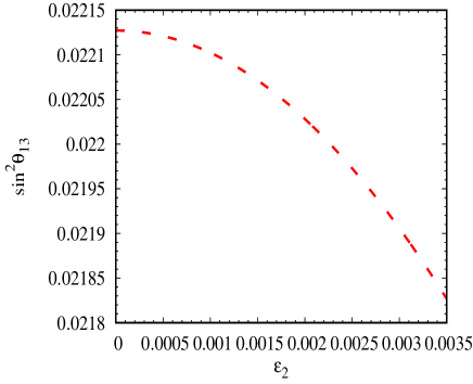
(c)

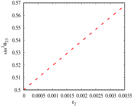
Figure 3: Plots of $\sin^{2}\theta_{ij}$ vs. $\varepsilon_{2}$ for the central values of IH ($b\equiv 0$) neutrino mass matrix elements.

VIII Conclusion

We have considered the constraints imposed by the precision oscillation data on $\mu\leftrightarrow\tau$ symmetric neutrino mass matrix. We find that the elements of this matrix are confined to be in extremely narrow ranges by the current data, both for normal hierarchy and for inverted hierarchy. There are two parameters which break the $\mu\leftrightarrow\tau$ symmetry, $\varepsilon_{1}$ and $\varepsilon_{2}$. Even though $\varepsilon_{1}$ is small, it can not be treated as a perturbation because its value is comparable (for NH) or much larger than (for IH) the relevant element of neutrino mass matrix. A value of $\varepsilon_{1}\sim 0.005$ eV (for both NH and IH) leads to a viable value of $\theta_{13}$ and only minimal deviation of $\theta_{23}$ away from maximality. The other parameter, $\varepsilon_{2}$ leads to very tiny values of $\theta_{13}$ but to substantial deviation of $\theta_{23}$ from maximality. Thus, the values of $\varepsilon_{1}$ and $\varepsilon_{2}$ are determined by the magnitude of $\theta_{13}$ and the deviation of $\theta_{23}$ from maximality respectively. In the case of $\mu\leftrightarrow\tau$ symmetry, we find that six parameters of neutrino mass matrix are needed to predict the five neutrino oscillation parameters and the lowest neutrino mass. On the other hand, it is possible to obtain viable values for the three neutrino masses and three mixing angles in terms of five parameters by imposing $\mu\leftrightarrow-\tau$ exchange symmetry for the case of IH. However, a fine-tuned cancellation among these parameters is required to obtain the measured value $\theta_{12}$.

References

Cleveland et al. (1998)
B. T. Cleveland,
T. Daily,
R. Davis, Jr.,
J. R. Distel,
K. Lande,
C. K. Lee,
P. S. Wildenhain,
and J. Ullman,
Astrophys. J. 496,
505 (1998).
Fukuda et al. (1996)
Y. Fukuda et al.
(Kamiokande), Phys. Rev. Lett.
77, 1683 (1996).
Abdurashitov et al. (1994)
D. Abdurashitov
et al. (SAGE), Phys.
Lett. B328, 234
(1994).
Hampel et al. (1999)
W. Hampel et al.
(GALLEX), Phys. Lett.
B447, 127 (1999).
Altmann et al. (2005)
M. Altmann et al.
(GNO), Phys. Lett.
B616, 174 (2005),
eprint hep-ex/0504037.
Abe et al. (2016)
K. Abe et al.
(Super-Kamiokande), Phys. Rev.
D94, 052010
(2016), eprint 1606.07538.
Bahcall et al. (2001)
J. N. Bahcall,
M. C. Gonzalez-Garcia,
and
C. Pena-Garay,
JHEP 08, 014
(2001), eprint hep-ph/0106258.
Casper et al. (1991)
D. Casper et al.,
Phys. Rev. Lett. 66,
2561 (1991).
Nakahata et al. (1986)
M. Nakahata et al.
(Kamiokande), J. Phys. Soc. Jap.
55, 3786 (1986).
Ashie et al. (2005)
Y. Ashie et al.
(Super-Kamiokande), Phys. Rev.
D71, 112005
(2005), eprint hep-ex/0501064.
(b)
(b) (c)
(c)
(b)
(b) (c)
(c)