Symmetry enhancement and closing of knots in 3d/3d correspondence

Abstract

We revisit Dimofte-Gaiotto-Gukov’s construction of 3d gauge theories associated to 3-manifolds with a torus boundary. After clarifying their construction from a viewpoint of compactification of a 6d ${\cal N}=(2,0)$ theory of $A_{1}$-type on a 3-manifold, we propose a topological criterion for $SU(2)/SO(3)$ flavor symmetry enhancement for the $u(1)$ symmetry in the theory associated to a torus boundary, which is expected from the 6d viewpoint. Base on the understanding of symmetry enhancement, we generalize the construction to closed 3-manifolds by identifying the gauge theory counterpart of Dehn filling operation. The generalized construction predicts infinitely many 3d dualities from surgery calculus in knot theory. Moreover, by using the symmetry enhancement criterion, we show that theories associated to all hyperboilc twist knots have surprising $SU(3)$ symmetry enhancement which is unexpected from the 6d viewpoint.

1 Introduction and Summary

3-dimensional (3d) quantum field theory exhibits several interesting aspects. Unlike higher dimensional case, Abelian gauge interaction in 3d is strongly coupled at infrared (IR) and gives non-trivial IR physics. Different gauge theories at ultraviolet (UV) could end at the same IR fixed point along renormalization group (RG) and such phenomena is called “duality”. Refer to Intriligator:1996ex ; deBoer:1996mp ; Aharony:1997bx for examples of dualities among 3d gauge theories. There could be enhanced symmetries in the IR fixed point which is invisible in the UV gauge theory. From purely field theoretic viewpoint, these phenomena are not easy to understand or predict.

In this paper, we consider a certain subclass of 3d quantum field theories with $\mathcal{N}=2$ (4 supercharges) supersymmetry which can be engineered by a twisted compactification of the 6d $(2,0)$-superconformal field theory (SCFT) of $A_{1}$ type. The 6d theory is the simplest maximally supersymmetric conformal field theory and describes the low energy world volume theory of two coincident M5-branes in M-theory. The 6d theory has $SO(5)$ R-symmetry and allows a 1/2 BPS regular co-dimension two defect. The concrete set-up of this paper is as follows

$$\begin{split}&\textrm{6d $A_{1}$ (2,0)-SCFT on $\mathbb{R}^{1,2}\times M$ with a partial topological twisting along $M$ }\\ &\textrm{with a regular co-dimension two defect along $\mathbb{R}^{1,2}\times K$}\\ &\xrightarrow[\text{}]{\quad\text{compacitification along $M$}\quad}T^{6d}[M,K]\textrm{ on $\mathbb{R}^{1,2}$}\;.\end{split}$$ (1)

Here $M$ is a compact (closed) 3-manifold and $K$ is a knot inside $M$. Using the vector $SO(3)$ subgroup of $SO(5)$ R-symmetry, we perform a topological twisting along $M$ which preserves $1/4$ supersymmetries. After the compactification, we obtain a 3d $\mathcal{N}=2$ quantum field theory, say $T^{6d}[M,K]$, determined by the topological choice of $M$ and $K$. These theories are 3d analogy of 4d $\mathcal{N}=2$ theories of class S Gaiotto:2009we ; Gaiotto:2009hg . In the analogy, closed Riemann surface corresponds to $M$ and a regular puncture on the surface corresponds to $K$. The 6d picture predicts the existence of $su(2)$ flavor symmetry associated to the knot in the resulting 3d gauge theory.

One non-trivial task is finding field theoretical description of the 3d theory $T^{6d}[M,K]$. A hint comes from so called 3d/3d relations Yagi:2013fda ; Cordova:2013cea ; Lee:2013ida ; Dimofte:2014zga ; Gang:2015wya which says that the partition functions of the $T^{6d}[M,K]$ theory on supersymmetric curved backgrounds are equal to the partition functions of purely bosonic $SL(2,\mathbb{C})$ Chern-Simons (CS) theories on $M$ with a monodromy defect along $K$. State-integral models 2007JGP ; Dimofte:2011gm ; Andersen:2011bt ; Dimofte:2012qj ; Dimofte:2014zga give integral expressions for complex CS partition functions while localization techniques Kim:2009wb ; Kapustin:2009kz ; Hama:2010av ; Imamura:2011su give similar integral expressions for the supersymmetric partition functions of 3d field theories.

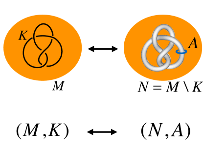
Figure 1: The choice of a knot $K$ inside a closed 3-manifold $M$ can be alternatively described by a choice of knot complement $N$ and a boundary cycle $A\in H_{1}(\partial N,\mathbb{Z})$.

Base on the technical developments, field theoretic algorithm of constructing 3d gauge theory $T^{DGG}[M,K]$ labelled by the choice of $(M,K)$ is proposed by Dimoft-Gaiotto-Gukov Dimofte:2011ju . Their construction guarantees that the localization integrals of the $T^{DGG}[M,K]$ theory are identical to the corresponding state-integral models. In the original paper, the 3d gauge theory $T^{DGG}[N,X_{A}]$ is actually labelled by a choice of a knot complement $N$ and a primitive boundary cycle $A\in H_{1}(\partial N,\mathbb{Z})$. But there is a one-to-one map between the two topological choices, $(M,K)$ and $(N,A)$, and we can labell them by the choice of $(M,K)$ which has more clear meaning in the 6d compactification (1). The explicit map between two topological choices is explained around Figure 1. From the non-trivial match of supersymmetric partition functions, it is tempting to conclude that the $T^{DGG}[M,K]$ is actually $T^{6d}[M,K]$. However, there are two manifest differences between two theories. Firstly, only some subset of irreducible flat $SL(2,\mathbb{C})$ connections on the knot complement $N:=M\backslash K$ appears as vacua on $\mathbb{R}^{2}\times S^{1}$ of $T^{DGG}[M,K]$ theory while all flat connections are expected to appear as the vacua of $T^{6d}[M,K]$ theory. This point was already emphasized in Chung:2014qpa . Secondly, the $T^{DGG}[M,K]$ theory generically has $U(1)$ flavor symmetry, denoted as $U(1)_{X_{A}}$, associated to the knot $K$ while $T^{6d}[M,K]$ has a $su(2)$ flavor symmetry. Motivated from the similarity and differences of two theories, we propose the precise relation (124) between them, which we reproduce here:

$$T^{6d}\xrightarrow[\text{}]{\textrm{\quad on a vacuum $P_{\rm SCFT}$}\quad}T^{6d}_{\rm irred}\xrightarrow[\text{}]{\textrm{\quad deformed by $\delta W=\mu^{3}$}\quad}T^{DGG}$$ (2)

Here $\mu=(\mu^{1},\mu^{2},\mu^{3})$ is a chiral operator in the triplet representation of $su(2)$, and this operator is associated the co-dimension two defect along $K$. Each of the arrows in the above equation are nontrivial RG flows which are explained below.

The proposed relation explains why the $T^{DGG}[M,K]$ theory generically has only $U(1)$ symmetry associated to the knot while $T^{6d}[M,K]$ has $su(2)$ flavor symmetry. The $su(2)$ symmetry of $T^{6d}[M,K]$ is broken by the superpotential deformation $\delta W=\mu^{3}$ in (2) which is typically a relevant deformation in the RG sense. After $S^{1}$-reduction, the 6d theory becomes 5d maximally supersymmetric $su(2)$ Yang-mills theory (SYM) and the co-dimension two defect in 6d theory is realized by coupling a copy of the 3d $\mathcal{N}=4$ $T[SU(2)]$ theory Gaiotto:2008ak to the 5d theory. Then $\mu$ is the $su(2)$ moment map operator of the 3d ${\cal N}=4$ $T[SU(2)]$ theory.

As an intermediate step, we introduce a 3d SCFT $T^{6d}_{\rm irred}[M,K]$ appearing in (2) which is the IR fixed point of $T^{6d}[M,K]$ on a particular point $P_{SCFT}$ of the vacuum moduli space. Unlike $T^{6d}[M,K]$, $T^{6d}_{\rm irred}[M,K]$ might not contain the $su(2)$ moment map operator $\mu$ after taking the IR limit. In that case, the superpotential deformation is not possible (or more precisely, it is irrelevant) and thus the $T^{DGG}[M,K]$ still has the $su(2)$ symmetry. By carefully analyzing the coupled system, 5d SYM+3d $T[SU(2)]$, we find a topological condition on $(N,A)$ which guarantees the absence of moment map operator and thus the $su(2)$ symmetry in $T^{DGG}[N,X_{A}]$ theory. The topological condition is summarized in Table 1. For example, we expect $su(2)$ symmetry enhancement when $M$ is a Lens-space and do not expect the enhancement when $M$ is hyperbolic.

As an application of the symmetry enhancement criterion, we show that the $T^{DGG}[M=S^{3},K]$ theory for all hyperbolic twist knots $K$ has a surprising $SU(3)$ symmetry. As a simplest example, we claim that the following 3d $\mathcal{N}=2$ theory has $SU(3)$ symmetry.

$$\begin{split}&T^{DGG}[M=S^{3},K=\textrm{figure-eight knot}]\\ &=\textrm{A $U(1)_{0}$ vector multiplet coupled to two chiral multiplets of charge +1}\;.\end{split}$$ (3)

The theory only has manifest $SU(2)\times U(1)$ symmetry where the $SU(2)$ rotates the two chirals and the $U(1)$ comes from the topological symmetry of the dynamical abelian gauge field. The $U(1)_{X_{A}}$ symmetry associated to the knot is a linear combination of two Cartans of the $SU(2)\times U(1)$ which is expected to be enhanced to $SO(3)$ according to the criterion in Table 1. From a group theoretical analysis, the enhancement implies that the $SU(2)\times U(1)$ should be enhanced to $SU(3)$. We checked the symmetry enhancement by explicitly constructing the corresponding conserved current multiplet.

Base on the proposed relation between $T^{6d}[M,K]$ and $T^{DGG}[M,K]$, we identify the field theoretical operation on $T^{DGG}[M,K]$ corresponding to Dehn filling operation on the knot complement $N=M\backslash K$. The operation is only possible when the $T^{DGG}[M,K]$ has $su(2)$ flavor symmetry. The Dehn filling operation is analogous to closing of punctures on Riemann surface in 4d/2d correspondence Tachikawa:2013kta . By applying the Dehn filling operation, we can extend the DGG’s construction to 3d gauge theories labelled by a closed 3-manifold $M$. The theory is denoted as $T^{6d}_{\rm irred}[M]$ and has similar 6d interpretation as $T^{6d}_{\rm irred}[M,K]$. As concrete examples, field theoretic descriptions of $T^{6d}_{\rm irred}[M]$ for three smallest hyperbolic 3-manifolds are given in Gang:2017lsr . One interesting aspect of our construction of $T^{6d}_{\rm irred}[M]$ is that we can relate surgery calculus in knot theory to 3d $\mathcal{N}=2$ dualities. One way of representing closed 3-manifold is using so called Dehn surgery representation. A closed 3-manifold $M$ has infinitely many different surgery descriptions and surgery calculus tell when two surgery descriptions give the same 3-manifold. Different surgery representations of a closed 3-manifold give different field theoretical descriptions of $T^{6d}_{\rm irred}[M]$ which are related by 3d dualities. One illustrative example is given around eq. (234). Since the 3d theory depends on only the topology of the 3-manifold, every physical quantities of the theory are topological invariants of the 3-manifold. As an example, we introduce a new 3-manifold invariant called “3d index” which is nothing but the superconformal index of the $T^{6d}_{\rm irred}[M]$.

The paper is organized as follows. In section 2, we introduce two ways of associating the choice of 3-manifold $M$ and a knot $K$ inside it with a 3d gauge theory $T[M,K]$. One is through the construction by Dimofte-Gaiotto-Gukov Dimofte:2011ju (DGG) and the corresponding gauge theory is denoted as $T^{DGG}[M,K]$. The other is through a twisted compactification of 6d $A_{1}$ (2,0) theory on $M$ with a regular co-dimension two defect along $K$. The resulting 3d gauge theory is denoted as $T^{6d}[M,K]$. After explaining the two constructions in detail, we propose a precise relation (124) between two constructions. Base on the proposed relation, in section 3, we give a topological criterion on $(M,K)$ which determines when the $U(1)_{X_{A}}$ symmetry $T^{DGG}[M,K]$ theory is enhanced to $SU(2)$ or $SO(3)$. The criterion is summarized in Table 1. In section 4, we identify field theoretic operation corresponding to Dehn filling operation in 3-manifold side in 3d/3d correspondence. It allows us to extend the DGG’s construction to the case when the knot is absent. In section 5, we discuss how the surgery calculus in knot theory predicts infinitely many 3d $\mathcal{N}=2$ dualities.

2 3d $\mathcal{N}=2$ Superconformal field theories labelled by 3-manifolds

In this section, we introduce two ways of associating a 3-manifold $M$ with a knot $K$ in it to a 3d $\mathcal{N}=2$ gauge theory $T[M,K]$.

$$\begin{split}&(M,K)\;\rightsquigarrow\;(\textrm{a 3d $\mathcal{N}=2$ gauge theory $T[M,K]$})\;,\textrm{ where}\\ &\textrm{$M$ is a closed 3-manifold}\;,\quad\textrm{$K\subset M$ is a knot in $M$}\;.\end{split}$$ (4)

One way is through a twisted compactification of a 6d $\mathcal{N}=(2,0)$ theory of $A_{1}$ type on a closed 3-manifold $M$ with a regular co-dimension two defect along a knot $K$ on $M$. The other way is using the construction by Dimofte-Gaiotto-Gukov Dimofte:2011ju (DGG) based on an ideal triangulation of the knot complement $M\backslash K$. These two theories are argued to be related Dimofte:2011ju , and we will propose the more precise relation between them with supporting evidences. We describe the relation after reviewing basic aspects of two approaches.

Before going to detailed analysis, let us first introduce an alternative labelling for the topological choice, ($M$ and $K$), which will be used throughout the paper.

The choice can be replaced by

$$\begin{split}&(M,K)\leftrightarrow(N,A)\;,\textrm{ where}\\ &\textrm{$N$ is a knot complement and $A\in H_{1}(\partial N,\mathbb{Z})$ is a primitive boundary cycle .}\end{split}$$ (5)

For a given $(M,K)$, the corresponding $(N,A)$ is given by

$$\begin{split}&N=M\backslash K:=M-N_{K}\;,\quad(N_{K}\textrm{ : Tubular neighborhood of a knot $K$})\\ &A\;:\;\textrm{A primitive boundary cycle around the knot $K$. }\\ &\qquad\textrm{(i.e. the contractible cycle in the removed tubular neighborhood $N_{K}$)}\end{split}$$ (6)

For given $(N,A)$, on the other hand, $(M,K)$ is determined by

$$\begin{split}M&=N_{A}:=(\textrm{A closed 3-manifold obtained from $N$ by closing a cycle $A$ in $\partial N$})\\ &:=(N\cup(D_{2}\times S^{1}))/\sim\;\;\textrm{with }A\sim\textrm{(contractible boundary cycle of $D_{2}\times S^{1}$)}\\ K&:=\{p\}\times S^{1}\subset D_{2}\times S^{1},\text{ where $p\in D_{2}$ is the origin of $D_{2}$.}\end{split}$$ (7)

Using the map, we can use two choices interchangeably. For example,

$$T[N,A]=T[M,K]\;.$$ (8)

In most part of this paper, we assume that $N$ is a knot complement with one torus boundary but our discussion can be easily generalized to the case when $N$ is a link complement with several torus boundaries.

2.1 6d $A_{1}$ (2,0) theory on 3-manifolds : $T^{6d}$ and $T^{6d}_{\rm irred}$

We define

$$\begin{split}&T^{6d}[M,K]=(\textrm{Twisted compactification of 6d (2,0) $A_{1}$ theory on $M$}\\ &\qquad\qquad\quad\qquad\textrm{with a regular co-dimension two defect along $K\subset M$})\;.\end{split}$$ (9)

$$\begin{split}&T^{6d}_{\rm irred}[M,K]=(\textrm{The low energy limit of $T^{6d}[M,K]$ }\\ &\qquad\qquad\quad\qquad\textrm{on a particular point $P_{\rm SCFT}$ on the moduli space of vacua})\;.\end{split}$$ (10)

As a simpler set-up, we can also consider the case when the defect is absent. In that case, the resulting 3d theory is denoted as $T^{6d}[M]$ and $T^{6d}_{\rm irred}[M]$, respectively. For the $T^{6d}_{\rm irred}[M,K]$ to be defined, we assume that $N=M\backslash K$ is a hyperbolic knot complement.

The reason that we consider $T^{6d}_{\rm irred}[M,K]$ is as follows. The moduli space of vacua of $T^{6d}[M,K]$ in general contains several different connected components. Then, we have to decide which point of the moduli space we consider before taking the low energy limit. The typical distances between different components of the moduli space are of the order of the compactification scale on $M$, which set the cutoff scale of the low energy effective 3d theory. Therefore, we cannot expect that there is a single effective 3d theory which describes the entire moduli space of vacua. Only after specifying a point on the moduli space, we can obtain a low energy effective field theory which describes the physics near that point.

In other words, $T^{6d}[M,K]$ is not a genuine 3d theory, but should be considered more appropriately as the 6d theory compactified on $M$. However, we will be sometimes sloppy and call it a 3d theory in this paper.

In $T^{6d}_{\rm irred}[M,K]$, we pick up a point and take the low energy limit. The low energy limit may be described by a 3d SCFT (which can be empty or a topological theory). Below we will specify which point on the moduli space of vacua we take, by using reduction to 5d SYM.

$T^{6d}$ on $\mathbb{R}^{2}\times S^{1}$ via 5d SYM

The structure of the moduli space of vacua becomes simpler if we compactify the 3d spacetime to ${\mathbb{R}}^{2}\times S^{1}$. This is because we can use the 5 dimensional maximally supersymmetric Yang-Mills (5d SYM) theory description. The set-up is

(11)

The bosonic components of the 5d SYM theory are gauge fields $A_{I}~{}(I=0,\cdots,4)$ and scalar fields $\phi_{k}~{}(k=0,\cdots,4)$. After compactification on $M$, the supersymmetry is defined on $\mathbb{R}^{2}$, and we split these fields as

$$(A_{I=0,1,2,3,4},\phi_{k=1,2,3,4,5})\to(A_{\mu=0,1},\phi_{k=0,1})\oplus(\mathcal{A}_{i}:=A_{i}+i\phi_{i})_{i=2,3,4}$$ (12)

From the point of view of the super-algebra on ${\mathbb{R}}^{2}$, the ${\cal V}=(A_{\mu=0,1},\phi_{k=0,1})$ is the vector multiplet and $\mathcal{A}_{i}=A_{i}+i\phi_{i}~{}(i=2,3,4)$ are twisted chiral fields. The reason that we regard $\mathcal{A}$ as twisted chiral fields rather than chiral fields is that the relation between 5d SYM and $T^{6d}[M]$ is a kind of mirror symmetry analogous to the case of 4d class S theories.

The twisted superpotential is given by complex Chern-Simons action as

$$\widetilde{W}_{\text{YM}}=\frac{1}{g_{\rm YM}^{2}}CS[\mathcal{A}]:=\frac{1}{g_{\rm YM}^{2}}\int_{M}\frac{1}{2}\mathrm{Tr}\left(\mathcal{A}d\mathcal{A}+\frac{2}{3}\mathcal{A}^{3}\right).$$ (13)

where $g_{\rm YM}^{2}$ is the gauge coupling of 5d SYM which is related to the radius $R$ of $S^{1}$ as

$$\frac{1}{g_{\rm YM}^{2}}=\frac{1}{8\pi^{2}R}.$$ (14)

This is the results in Yagi:2013fda ; Lee:2013ida ; Cordova:2013cea in the limit $S^{2}\to\mathbb{R}^{2}$. This twisted superpotential corresponds to the twisted superpotential obtained in DGG’s construction discussed in Sec. 2.2

The regular co-dimension two defect along a knot $K\subset M$ can be realized as coupling the 3d $T[SU(2)]$ theory Gaiotto:2008ak to the fields of 5d SYM Benini:2009gi ; Benini:2010uu ; Gaiotto:2011xs ; Chacaltana:2012zy ; Yonekura:2013mya . The theory $T[SU(2)]$ is reviewed in Appendix B.1. This is a 3d $\mathcal{N}=4$ SCFT given by $U(1)$ vector multiplet coupled two fundamental hypermultiplets $(E^{a},\tilde{E}_{a})_{a=1,2}$. The theory has $su(2)_{H}\times su(2)_{C}$ flavor symmetry and let

$$\begin{split}&\widetilde{\mu}:=\textrm{holomorphic moment map operator of $su(2)_{C}$}\;,\\ &\widetilde{\nu}:=\textrm{holomorphic moment map operator of $su(2)_{H}$}\;.\end{split}$$ (15)

Then the twisted superpotential coupling of the $T[SU(2)]$ and the 5d SYM is given by

$$\widetilde{W}_{\text{YM-defect}}=\int_{K}\textrm{tr}(\widetilde{\nu}\mathcal{A}).$$ (16)

This means that we integrate the one-form $\textrm{tr}(\widetilde{\nu}\mathcal{A}_{i})dy^{i}$ over $K$.

We can also include (complexified) mass terms to the defect as

$$\widetilde{W}_{\rm mass}=\int_{K}ds\;\textrm{tr}(m\widetilde{\mu})$$ (17)

where $ds$ is the line element on $K$, and $m$ is the mass. The mass of defect is related to the eigenvalues of $\widetilde{\nu}$:

$$\textrm{Eigenvalues of $\widetilde{\nu}$}=\{m,-m\}\;.$$ (18)

See Yonekura:2013mya for detailed explanations of the coupling of 5d SYM to $T[SU(2)]$ in the context of 4d class S theories. The analysis there may be extended to the 3d/3d case, but we do not perform a detailed analysis.

By solving F-term equations for the twisted superpotenal in (13) and (16), a part of the moduli space of vacua on $\mathbb{R}^{2}\times S^{1}$ with mass parameter $m$ is given by

$$\begin{split}&\mathcal{M}_{\rm vacua}(\textrm{$T^{6d}[M,K]$ on $\mathbb{R}^{2}\times S^{1}$})\\ &=\{\mathcal{A}:d\mathcal{A}+\mathcal{A}\wedge\mathcal{A}=\widetilde{\nu}\delta(K),~{}\text{eigenvalues of }\widetilde{\nu}=\{m,-m\}\}/{\cal G}\;.\end{split}$$ (19)

where $\delta(K)$ is the delta function localized on $K$, and ${\cal G}$ is the group of $PSL(2,\mathbb{C})$ gauge transformations on $M$. This is the space of flat connections of the complexifield gauge group $PSL(2,\mathbb{C})$ with the holonomy $e^{\widetilde{\nu}}$ around $K$.

$$\rho_{\rm hol}(A):=(\textrm{$PSL(2,\mathbb{C})$ holonomy matrix along $A$-cycle})=e^{\widetilde{\nu}}\;.$$ (20)

Notice that the eigenvalues of $e^{\widetilde{\nu}}$ are determined by the mass parameter $m$.

Now we can specify the point $P_{\rm SCFT}$ on the moduli space of vacua which is taken in the definition (10). First, let us consider more generally. For simplicity we assume that the moduli space of vacua on ${\mathbb{R}}^{3}$, $\mathcal{M}_{\rm vacua}(\textrm{$T^{6d}[M,K]$ on $\mathbb{R}^{3}$})$, is a discrete set. Let us take an arbitary point $P\in\mathcal{M}_{\rm vacua}(\textrm{$T^{6d}[M,K]$ on $\mathbb{R}^{3}$ })$. Then, if we compactify the theory on $S^{1}$ with a radius which is large enough compared to potential barriers between different points on $\mathcal{M}_{\rm vacua}(\textrm{$T^{6d}[M,K]$ on $\mathbb{R}^{3}$})$, then the point $P$ goes to a subset ${\cal M}(P)$ of the moduli space of vacua on ${\mathbb{R}}^{2}\times S^{1}$ denoted as $\mathcal{M}_{\rm vacua}(\textrm{$T^{6d}[M,K]$ on $\mathbb{R}^{2}\times S^{1}$})$,

$$P\to{\cal M}(P)\subset\mathcal{M}_{\rm vacua}(\textrm{$T^{6d}[M,K]$ on $\mathbb{R}^{2}\times S^{1}$}).$$ (21)

This ${\cal M}(P)$ need not be a single point, but may have several points whose number is related to the Witten index of the 3d effective theory on $P$. Because of the supersymmetry, the condition that the radius of $S^{1}$ is large may be dropped since there is no phase transition under change of the radius.

The explicit forms of $\mathcal{M}_{\rm vacua}(\textrm{$T^{6d}[M,K]$ on $\mathbb{R}^{3}$})$ and ${\cal M}(P)$ are not known and they are defined just by the abstract field theoretical considerations as above. However, later we will propose how ${\cal M}(P_{\rm SCFT})$ may be given concretely in terms of flat $PSL(2,{\mathbb{C}})$ connections.

To consider a superconformal point, we set the mass $m$ to be zero. Then the point $P_{\rm SCFT}$ is defined as follows. After compactification on $S^{1}$, the moduli space of vacua of the theory on $P_{\rm SCFT}$ becomes a subset ${\cal M}(P_{\rm SCFT})$ of the moduli space of vacua on ${\mathbb{R}}^{2}\times S^{1}$. Then, the point $P_{\rm SCFT}$ is defined by the condition that ${\cal M}(P_{\rm SCFT})$ contains the connection ${\cal A}^{\rm\overline{hyp}}\in\mathcal{M}_{\rm vacua}(\textrm{$T^{6d}[M,K]$ on $\mathbb{R}^{2}\times S^{1}$})$ which is determined by the unique complete hyperbolic metric on $N=M\backslash K$. More explicitly, using the spin-connection $\omega$ and dreibein $e$ of the complete hyperbolic metric, the flat connection can be expressed as

$${\cal A}^{\rm\overline{hyp}}=\omega-ie\;.$$ (22)

This flat connection has the greatest value of $\textrm{Im}(CS[{\cal A}^{\alpha}])$ among all flat connections ${\cal A}^{\alpha}$ with parabolic boundary holonomy and is conjectured to be the only vacua contributing to a squashed 3-sphere partition function Hama:2011ea of $T^{6d}_{\rm irred}[M,K]$. Refer to Andersen:2011bt ; Gang:2014ema ; Bae:2016jpi ; Mikhaylov:2017ngi ; Gang:2017hbs for discussions on the conjecture from various respects, state-integral model of the complex CS theory, holographic principal and resurgent analysis. To other physical quantities of $T^{6d}_{\rm irred}[M,K]$ such as superconformal index, on the other hand, other flat connections in ${\cal M}(P_{\rm SCFT})$ may contributes.

Now we give a conjecture about how ${\cal M}(P_{\rm SCFT})$ is given concretely in terms of flat connections. First we consider the case where a knot $K$ exists. For this purpose, we define ${\cal M}(P_{\rm SCFT})$ even for nonzero mass $m$ by continuity from $m=0$. Namely, ${\cal M}(P_{\rm SCFT})$ is just the set of vacua of the 3d effective theory near $P_{\rm SCFT}$ with mass $m$. We make the dependence on $m$ explicit by writing it as ${\cal M}(P_{\rm SCFT},m)$. We also define $\chi(N)$ as

$$\chi(N)=\bigcup_{m}\{\mathcal{A}:d\mathcal{A}+\mathcal{A}\wedge\mathcal{A}=\widetilde{\nu}\delta(K),~{}\text{eigenvalues of }\widetilde{\nu}=\{m,-m\}\}/{\cal G}$$ (23)

This means that we consider all flat connections with varying holonomy around the knot. Then we propose

$$\bigcup_{m}{\cal M}(P_{\rm SCFT},m) =\;\{\textrm{the connected component of $\chi(N)$ containing ${\cal A}^{\rm\overline{hyp}}$}\}$$

$$:=\chi_{0}(N)\;.$$ (24)

In tillmann2012degenerations , the component is called Dehn surgery component. Another way of representing the above equation is ${\cal M}(P_{\rm SCFT},m)=\chi_{0}(N)\cap\{\text{eigenvalues of }\nu=\{m,-m\}\}$.

Next, consider the case where there is no knot on $M$. If the closed 3-manifold is represented by a Dehn filling operation on a hyperbolic knot complement $N=M\backslash K$ for some $K$ along a boundary cycle $A$,

$$M=N_{A}$$ (25)

we propose that the ${\cal M}(P_{\rm SCFT})$ is given by

$${\cal M}(P_{\rm SCFT})\textrm{ of the closed manifold }M$$

$$=\chi_{0}(N)\cap\{\rho_{\rm hol}(A)=1\}$$ (26)

The definition of the right hand side contains a knot $K$, but we assume that it is independent of the choice $K\subset M$. Notice that $\rho_{\rm hol}(A)=1$ is stronger than $m=0$, since we could have a nonzero upper-right component of $\nu$ even if its eigenvalues are zero.

2.2 Dimofte-Gaiotto-Gukov’s construction : $T^{DGG}$

In Dimofte:2011ju , a combinatorial way of constructing a 3d SCFT, which we denote $T^{DGG}[N,X_{A}]$, for given choice of $(N,A)$ is proposed. Empirically, the theory associated to non-hyperbolic $N$ is a trivial theory only with topological degrees of freedom. In this subsection we focus on the case when $N$ is hyperbolic. Here we give a summary of the DGG’s construction with a modification on superpotential deformation associated to ‘hard’ internal edges (see (72)) which play a crucial role in the symmetry enhancement of the theory.

Mechanics of ideal triangualtion

The construction is based on a choice of an ideal triangulation $\mathcal{T}$ of $N$.

$$\mathcal{T}\;:\;N=\bigg{(}\bigcup_{i=1}^{k}\Delta_{i}\bigg{)}/\sim\;.$$ (27)

Here $\Delta_{i}$ denote the $i$-th tetrahedron in the triangulation. Ideal tetrahedron can be embedded into a hyperbolic upper half plane $\mathbb{H}^{3}$ in a way that all vertices are located on the boundary of $\mathbb{H}^{3}$ and both of edges and faces are geodesics. Hyperbolic structures on an ideal tetrahedron can be parameterized by a complex parameter $z$ (with $0<\textrm{Im}[Z]<\pi$, $Z:=\log z$), which is the cross-ratio of the positions of its vertices on $\partial\mathbb{H}^{3}$. We assign edge parameters $(z,z^{\prime},z^{\prime\prime})$ to each pair of edges of ideal tetrahedron as in the figure below.

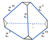
Figure 2: Edge parameters $(z,z^{\prime},z^{\prime\prime})$ of an ideal tetrahedron. Left: ideal tetrahedron in $\mathbb{H}^{3}=\{(y,w):y\in\mathbb{R}_{+},w\in\mathbb{C}\}$ with metric $ds^{2}(\mathbb{H}^{3})=\frac{dy^{2}+dwd\bar{w}}{y^{2}}$. Using the isometry of $\mathbb{H}^{3}$, $PSL(2,\mathbb{C})$, four asymptotic vertices can be placed at $(y,w)=(0,0),(0,1),(0,z)$ and $(\infty,\cdot)$. Right: topologically, ideal tetrahedron is a tetrahedron with truncated vertices.

Geometrically, these edge parameters correspond to

$$\{Z,Z^{\prime},Z^{\prime\prime}\}:=\{\log z,\log z^{\prime},\log z^{\prime\prime}\}$$

$$=i(\textrm{dihedral angle between two faces meeting on the edge})+(\textrm{torsion})\;.$$ (28)

Here “torsion” is a quantity which measures the twisting of hyperbolic metric around the edge. For an ideal tetrahedron in $\mathbb{H}^{3}$, these parameters satisfy

$$\begin{split}&Z_{i}+Z^{\prime}_{i}+Z^{\prime\prime}_{i}=i\pi\;(\textrm{sum of angles in small boundary triangle equals to $\pi$})\;,\\ &e^{-Z_{i}}+e^{Z^{\prime\prime}_{i}}=1\;.\end{split}$$ (29)

The second equation follows directly from the geometric definition of $(z,z^{\prime},z^{\prime\prime})$ as equivalent cross-ratios. These constraints are compatible with the following cyclic symmetry of ideal tetrahedron:

$$\mathbb{Z}_{3}\;:\;(Z,Z^{\prime},Z^{\prime\prime})\rightarrow(Z^{\prime},Z^{\prime\prime},Z)\rightarrow(Z^{\prime\prime},Z,Z^{\prime})\;.$$ (30)

An hyperbolic structure on a knot complement $N$ can be obtained by gluing the hyperbolic structure on each tetrahedron in a smooth way. For the smooth gluing, we need to impose the following conditions

$$\begin{split}C_{I}&:=(\textrm{sum of all logarithmic edge variables associated to }\\ &\quad\quad\textrm{edges meeting at the $I$-th internal edge in the gluing})\\ &=\sum_{i=1}^{k}(G_{Ii}Z_{i}+G^{\prime}_{Ii}Z^{\prime}_{i}+G^{\prime\prime}_{Ii}Z^{\prime\prime}_{i})\;,\quad G_{Ii},G^{\prime}_{Ii},G^{\prime\prime}_{Ii}\in\{0,1,2\}\;.\\ &=2\pi i\;.\end{split}$$ (31)

There are $k$-internal edges in an ideal triangulation with $k$ ideal tetrahedra. A solution to these gluing equations (29) and (31) with conditions $0<\textrm{Im}[Z_{i}]<\pi$ for all $i$ gives a hyperbolic (generally incomplete) structure on $N$.

${\cal M}(P_{SCFT})$ from ideal triangulation

More generally, a solution to the exponentiated gluing equations gives an irreducible flat $PSL(2,\mathbb{C})=SL(2,\mathbb{C})/\langle\pm 1\rangle$ connections on $N$. Consider the algebraic variety $\mathcal{D}[N,\mathcal{T}]$ determined by gluing equations of an ideal triangulation $\mathcal{T}$,

$$\mathcal{D}[N,\mathcal{T}]:=\{z_{i},z^{\prime}_{i},z^{\prime\prime}_{i}\in\mathbb{C}\backslash\{0,1\}:z_{i}z_{i}^{\prime}z_{i}^{\prime\prime}=-1,z_{i}^{-1}+z^{\prime\prime}_{i}-1=0,\prod_{i=1}^{k}z_{i}^{G_{Ii}}(z^{\prime}_{i})^{G^{\prime}_{Ii}}(z^{\prime\prime}_{i})^{G^{\prime\prime}_{Ii}}=1\}\;.$$ (32)

The variety is called a deformation variety. A point in $\mathcal{D}[N,\mathcal{T}]$ gives an irreducible flat-connection via a map $\chi_{T}$

$$\chi_{\mathcal{T}}:\;\mathcal{D}[N,\mathcal{T}]\rightarrow\chi(N):=\{\rho_{\rm hol}\in\textrm{Hom}\big{[}\pi_{1}(N)\rightarrow PSL(2,\mathbb{C})\big{]}/(\textrm{conj})\}\;.$$ (33)

where the definition of $\chi(N)$ here is equivalent to that in (23). The map $\chi_{\mathcal{T}}$ is injective but not surjective. Using the map, holonomy matrix along a primitive boundary cycle $A\in H_{1}(\partial N,\mathbb{Z})=\pi_{1}(\partial N)\subset\pi_{1}(N)$ can be written as linear combinations of logarithmic edge parameters

$$\begin{split}&\rho_{\rm hol}(A)=\left(\begin{array}[]{cc}e^{a/2}&0\\ &e^{-a/2}\end{array}\right)\quad\textrm{where }a=\sum_{i=1}^{k}(\alpha_{i}Z_{i}+\alpha^{\prime\prime}_{i}Z^{\prime\prime}_{i})+i\pi\epsilon\\ &\textrm{with integer coefficients }(\alpha_{i},\alpha^{\prime\prime}_{i},\epsilon)\;.\end{split}$$ (34)

Dependence on $\{Z^{\prime}_{i}\}$ was eliminated using the linear relations in (29). The algebraic variety depends on the choice of an ideal triangulation $\mathcal{T}$ of $N$. But it is known that the Dehn surgery component $\chi_{0}(N)=\bigcup_{m}{\cal M}(P_{SCFT},m)$ in (24) is always contained in $\mathcal{D}[N,\mathcal{T}]$ for any $\mathcal{T}$ except exotic cases when $\mathcal{D}[N,\mathcal{T}]$ is empty tillmann2012degenerations ,

$$\begin{split}\chi_{0}(N)=\;&\textrm{the connected component of $\mathcal{D}[N,\mathcal{T}]$ for non-exotic $\mathcal{T}$ }\\ &\textrm{containing a solution of gluing eqns corresponding to ${\cal A}^{\rm\overline{hyp}}$}\;.\end{split}$$ (35)

We currently do not have the field theoretic understanding of the exotic case and will always work with non-exotic triangulations.

$SU(2)/SO(3)$-type of boundary cycle $A$

For later use, we classify a primitive boundary cycle $A$ into two types, $SU(2)$ or $SO(3)$, depending on evenness/oddness of the linear coefficients $(\alpha_{i},\alpha^{\prime\prime}_{i})$.

$$A\textrm{ is of }\begin{cases}\textrm{$SU(2)$-type}\;,\;\textrm{if all $(\alpha_{i},\alpha^{\prime\prime}_{i})$ can be chosen as even-integers}\\ \textrm{$SO(3)$-type}\;,\;\textrm{otherwise}\end{cases}$$ (36)

Note that the linear coefficients are defined modulo the following shifts due to the last gluing equations in (32)

$$\bigg{(}\alpha_{i},\alpha^{\prime\prime}_{i}\bigg{)}\rightarrow\bigg{(}\alpha_{i}+\sum_{i=1}^{k}c_{Ii}(G_{Ii}-G^{\prime}_{Ii}),\alpha^{\prime\prime}_{i}+\sum_{i=1}^{k}c_{Ii}(G^{\prime\prime}_{Ii}-G^{\prime}_{Ii})\bigg{)}\quad\textrm{with some integers $c_{Ii}$}\;,$$

and $A$ is $SU(2)$-type if there is a choice of $c_{Ii}$ which makes all $(\alpha_{i},\alpha^{\prime\prime}_{i})$ even-integers. An alternative definition of $SO(3)/SU(2)$ type without relying an ideal triangulation is

$$A\textrm{ is of }\begin{cases}\textrm{$SU(2)$-type}\;,\;A\in\textrm{Ker}\big{(}i_{*}:H_{1}(\partial N,\mathbb{Z})\rightarrow H_{1}(N,\mathbb{Z}_{2})\big{)}\\ \textrm{$SO(3)$-type}\;,\;\textrm{otherwise}\end{cases}$$ (37)

Two definitions, (36) and (37), are equivalent neumann1992combinatorics . An explanation of $SU(2)/SO(3)$ types from the 6d ${\cal N}=(2,0)$ theory point of view is discussed in Appendix B.

$T^{DGG}[N,X_{A}]$ from symplectic gluing

The gluing equations are known to have the following symplectic structure neumann1985volumes ; neumann1992combinatorics which play a crucial role in the DGG’s construction. Upon a skew-symmetric bilinear $\{\;,\;\}$ defined by $\{Z_{i},Z^{\prime}_{j}\}=\{Z^{\prime}_{i},Z^{\prime\prime}_{j}\}=\{Z^{\prime\prime}_{i},Z_{j}\}=\delta_{ij}$, internal edge variables $\{C_{I}\}$ and the boundary holonomy variable $a$ around $A$ satisfy the followings:

$$\{C_{I},C_{J}\}=\{a,C_{I}\}=0\;,\quad\textrm{for all $I,J=1,\ldots,k$}$$ (38)

Further we can choose a linearly independent primitive cycle $B\in H_{1}(\partial N,\mathbb{Z})$ such that

$$\{a,b\}=-2\;,$$ (39)

where $b$ is related to the holonomy along $B$ as in eq. (34). The choice of $B$ is not unique but have the following freedom of choice

$$B\rightarrow B+kA\;,\quad k\in\mathbb{Z}\;.$$ (40)

Using the freedom, we will always choose $B$ to have the properties that

$$B\textrm{ is of }\begin{cases}\textrm{$SU(2)$ type}\;,\;\textrm{when $A$ is of $SO(3)$ type\;,}\\ \textrm{$SO(3)$ type}\;,\;\textrm{when $A$ is of $SU(2)$ type\;,}\end{cases}$$ (41)

where the $SU(2)/SO(3)$ types of $B$-cycle is defined in the same way as $A$.

Among $k$-internal edge variables in eq. (31), only $k-1$ of them are linearly independent modulo linear relations in (29). Let the linearly independent set as $\{C_{I}\}_{I=1}^{k-1}$. Then, we introduce their conjugate variables $\{\Gamma_{I}\}_{I=1}^{k-1}$ satisfying

$$\{C_{I},\Gamma_{J}\}=\delta_{IJ}\;,\quad\{a,\Gamma_{I}\}=\{b,\Gamma_{I}\}=0\;,\quad I,J=1,\ldots,k-1\;.$$ (42)

From the choice of $(A,B,\{C_{I}\},\{\Gamma_{I}\})$, we associate a $Sp(2k,\mathbb{Z})$ matrix $g_{N}$ and integer-valued $2k$-vector $\nu$ as follows

$$\left(\begin{array}[]{c}X_{A}\\ C_{1}\\ \ldots\\ C_{k-1}\\ P_{B}\\ \Gamma_{1}\\ \ldots\\ \Gamma_{k-1}\end{array}\right)=g_{N}\cdot\left(\begin{array}[]{c}Z_{1}\\ Z_{2}\\ \ldots\\ Z_{k}\\ Z_{1}^{\prime\prime}\\ Z_{2}^{\prime\prime}\\ \ldots\\ Z_{k}^{\prime\prime}\end{array}\right)+i\pi\nu_{N}\;,$$ (59)

where

$$(X_{A},P_{B})=\begin{cases}(\frac{a}{2},b)\;,\;\textrm{when $(A,B)$ is of $\big{(}SU(2),SO(3)\big{)}$ type}\\ (a,\frac{b}{2})\;,\;\textrm{when $(A,B)$ is of $\big{(}SO(3),SU(2)\big{)}$ type}\end{cases}$$ (60)

Notice that $(X_{A},P_{B})$ are always linear combinations of $Z_{i},Z^{\prime\prime}_{i}$ with integer coefficients because of the even-ness condition (36).

Using the gluing data summarized in $(g_{N},\nu_{N})$, we can construct the corresponding $T^{DGG}$ theory. As a first step, we prepare $k$-copies of a free chiral theory

$$\begin{split}&T_{\textrm{step I}}=T_{\Delta}^{\otimes k}=\overbrace{T_{\Delta}\otimes\ldots\otimes T_{\Delta}}^{\textrm{$k$ times}}\;,\\ &T_{\Delta}:=(\textrm{a free theory of single chiral multiplet $\Phi$ with CS level $-1/2$}\\ &\quad\quad\quad\textrm{ for non-dynamical background gauge field coupled to $U(1)$ flavor symmetry})\;,\\ &\mathcal{L}_{T_{\rm step1}}(V_{1},\ldots,V_{k})=\sum_{i=1}^{k}\frac{1}{4\pi}\int d^{4}\theta(-\frac{1}{2}\Sigma_{i}V_{i})+\int d^{4}\theta\Phi_{i}^{\dagger}e^{V_{i}}\Phi_{i}\;,\end{split}$$ (61)

where $\Sigma_{i}$ is the field strength of the vector multiplet $V_{i}$. The theory $T_{\textrm{step I}}$ has $u(1)^{k}$ flavor symmetry and $\{V_{i}\}$ are background vector-multiplets coupled to the flavor symmetries.

Using the symmetry, one can consider $Sp(2k,\mathbb{Z})$ action on the theory which is a generalization of Witten’s $SL(2,\mathbb{Z})$ action Witten:2003ya which corresponds to $k=1$ case. To be more explicit, one needs to decompose a $Sp(2k,\mathbb{Z})$ into products of “T-type ($g^{t}_{K}$),” “S-type ($g^{s}_{J}$),” and “GL-type($g^{gl}_{U}$)”:

$$g^{t}_{K}:=\left(\begin{array}[]{cc}I&0\\ K&I\end{array}\right)\ \;,\quad g^{s}_{J}:=\left(\begin{array}[]{cc}I-J&-J\\ J&I-J\end{array}\right)\ \;,\quad g^{gl}_{U}:=\left(\begin{array}[]{cc}U&0\\ 0&(U^{-1})^{t}\end{array}\right)\ \;.$$ (68)

Here $J$ is a diagonal matrix whose diagonal entries are either 0 or 1. Let $\mathcal{L}_{T}(\vec{V}:=(V_{1},\ldots,V_{k}))$ be a Lagrangian for a theory $T$ with $U(1)^{k}$ flavor symmetry. Field theoretic actions of the basic types are

$$\begin{split}&\mathcal{L}_{g^{t}_{K}\cdot T}(\vec{V}):=\mathcal{L}_{T}(\vec{V})+\frac{1}{4\pi}\int d^{4}\theta\vec{\Sigma}\cdot K\vec{V}\;,\\ &\mathcal{L}_{g^{s}_{J}\cdot T}(\vec{V}):=\mathcal{L}_{T}((I-J)\vec{V}+J\vec{V}^{\prime})+\frac{1}{2\pi}\int d^{4}\theta\vec{\Sigma}\cdot J\vec{V}^{\prime}\;,\\ &\mathcal{L}_{g^{gl}_{U}\cdot T}(\vec{V}):=\mathcal{L}_{T}(U^{-1}\cdot\vec{V})\;,\end{split}$$ (69)

where $\vec{V}^{\prime}$ only has components such that $J\vec{V}^{\prime}=\vec{V}^{\prime}$, and they are now dynamical fields. As for the $SL(2,\mathbb{Z})$ case, the final theory does not depend on the decomposition and depends only on the $Sp(2k,\mathbb{Z})$ element.

Now the second step of the construction is

$$T_{\textrm{step II}}=g_{N}\cdot T_{\textrm{step I}}\;,$$ (70)

where $g_{N}$ is the symplectic matrix in (59) obtained from an ideal triangulation of $N$. The $g_{N}$-transformed theory still has $u(1)^{k}$ flavor symmetry

$$U(1)_{X_{A}}\times U(1)_{C_{1}}\times\ldots\times U(1)_{C_{k-1}}\;,$$ (71)

whose background gauge fields are $V_{X_{A}}:=V_{1},\ldots,V_{C_{k-1}}:=V_{k}$ in $T_{\textrm{step II}}$.

As a final step, we break the $U(1)^{k}$ to its subgroup by adding chiral operators to the superpotential

$$\mathcal{L}_{T^{DGG}[N,X_{A}]}=\mathcal{L}_{T_{\textrm{step II}}}+\bigg{(}\sum_{\textrm{`easy' $C_{I}$}}\int d^{2}\theta O_{C_{I}}+c.c\bigg{)}\;.$$ (72)

An internal edge $C_{I}=\sum_{i=1}^{k}(G_{Ii}Z_{i}+G^{\prime}_{Ii}Z^{\prime}_{i}+G^{\prime\prime}_{Ii}Z^{\prime\prime}_{i})$ in (31) is called ‘easy’ Dimofte:2011ju if at most one of $G_{Ii}$, $G^{\prime}_{Ii}$ and $G^{\prime\prime}_{Ii}$ is nonzero for each $i$,

$$\sum_{i=1}^{k}(G_{Ii}G^{\prime}_{Ii}+G^{\prime}_{Ii}G^{\prime\prime}_{Ii}+G^{\prime\prime}_{Ii}G_{Ii})=0\;$$ (73)

and ‘hard’ otherwise. This condition simply means that only one of edge parameters ($Z_{i},Z^{\prime}_{i}$ and $Z^{\prime\prime}_{i}$) of $i$-th tetrahedron appears in $C_{I}$ for all $i=1\ldots k$. Upon a proper choice of cyclic relabeling (30) of edge parameters, we can make such an internal edge $C_{I}$ as a linear combination of only $Z_{i}$s:

$$C_{I}=\sum_{i=1}^{k}\widetilde{G}_{Ii}Z_{i}\;,\quad G_{Ii}\in\{0,1,2\}\;.$$ (74)

Then, the gauge-invariant chiral primary operator $O_{C_{I}}$ in $T_{\textrm{step II}}$ is given by

$$O_{C_{I}}=\prod_{i=1}^{k}\Phi_{i}^{\widetilde{G}_{Ii}}\;.$$ (75)

As will be explained below, different cyclic labelings give different descriptions of $T_{\textrm{step II}}$ which are related by a sequence of basic dualities in (81). Therefore for each easy internal edge $C_{I}$, there is a chiral primary operator $O_{C_{I}}$ which can be written as the above form in a duality frame. The operator is charged only under $U(1)_{C_{I}}$. For each hard internal edge, on the other hand, there may only be a corresponding gauge invariant dyonic 1/4 BPS operator with non-zero spin. There is no way to write down a supersymmetric deformation using the dyonic local operators.

Hard internal edges and accidental symmetries

In the original DGG’s construction Dimofte:2011ju , they proposed to use ideal triangulations with only easy internal edges. From superficial counting, we expect the resulting $T^{DGG}[N]$ has flavor symmetry of rank $1$ whose Cartan corresponds to the $U(1)_{X_{A}}$.

$$\begin{split}&\textrm{If all $C_{I}$ are easy, we superficially expect that}\\ &U(1)_{X_{A}}\times U(1)_{C_{1}}\times\ldots\times U(1)_{C_{k-1}}\;\textrm{in $T_{\textrm{step II}}$}\\ &\xrightarrow[]{\textrm{\quad Superpotential deformation in \eqref{DGG : final} \quad}}U(1)_{X_{A}}\;\textrm{in $T^{DGG}[N,X_{A}]$}\end{split}$$ (76)

The counting sounds compatible with the 6d construction since the knot gives a flavor symmetry $(su(2))$ of rank 1. But the counting could be wrong as we will see below for the case with an ideal triangulation of $N=(\textrm{figure-eight knot complement})$ with $6$-tetrahedra. The correct rank is always equal or greater than the superficial counting. In our modified proposal (72), we can use any ideal triangulation and will argue that the resulting theory is independent of the choice of ideal triangulation regardless of existence of hard edges. One of the consequences is that rank of the flavor symmetry could be larger than $1$ because the number of independent easy edges could be less than $(k-1)$. From the counting of linearly independent easy internal edges, we checked that $T^{DGG}$ theories for most of knot complements in SnapPy’s census have additional symmetries.

For example, we show the $SU(3)$ symmetry for all hyperbolic twist knots in section 3.2. The additional symmetries are accidental and unexpected from 6d viewpoint. The above DGG’s construction can be generalized to higher $\mathcal{K}$ (number of M5-branes) cases Dimofte:2014zga and there is no such an additional symmetry when $\mathcal{K}$ is sufficiently large. For higher ${\cal K}$ one need to use a so-called $\mathcal{K}$-decomposition which replace a single tetrahedron in an ideal triangulation into $\frac{1}{6}\mathcal{K}(\mathcal{K}^{2}-1)$ copies of finer building blocks, octahedra. The construction of the 3d theory for higher $\mathcal{K}$ is parallel to the construction for $\mathcal{K}=2$ case reviewed above except tetrahedra in an ideal triangulation are replaced by octahedra in a $\mathcal{K}$-decomposition. We assign 3 complex parameters ($z,z^{\prime},z^{\prime\prime}$) to each pair of two vertices of an octahedron and their gluing equations in a ${\cal K}$-decomposition also possess a symplectic structure. One difference in higher $\mathcal{K}$ is that there are enough number of easy internal edges (better to call internal vertices for $\mathcal{K}$-decomposition case) to break all $u(1)$ symmetries except the ones expected from 6d viewpoint. 6d viewpoint expect that the 3d theory has a flavor symmetry of rank $(\mathcal{K}-1)$. A hard internal edge appears when two edges of a single tetrahedron are glued to the internal edges simultaneously. In $\mathcal{K}$-decomposition, two different vertices of a single octahedron can not meet at an internal vertex possibly except when the octahedron is located nearest to one of vertices of tetrahedrons. So the number of hard internal vertices will be at most order of $k$ (the number of tetrahedrons in a triangulation) while there are $k\frac{\mathcal{K}(\mathcal{K}^{2}-1)}{6}$ internal vertices among which $(\mathcal{K}-1)$ are linearly dependent. So the number of easy internal vertices are $k\big{(}\frac{\mathcal{K}(\mathcal{K}^{2}-1)}{6}-o(1)\big{)}$ which is large enough to span the $\big{(}k\frac{\mathcal{K}(\mathcal{K}^{2}-1)}{6}-(\mathcal{K}-1)\big{)}$-linearly independent internal vertices for sufficiently large $\mathcal{K}$.

Topological invariance of $T^{DGG}[N,X_{A}]$

At first glance, the above construction seems to depend on the various choices other than $(N,A)$. For the construction, we choose an ideal triangulation of $N$. All different ideal triangulations of a given 3-manifold are known to be related by sequence of a basic local move called 2-3 Pachner move. In the DGG’s construction, the geometric move corresponds to a mirror symmetry between a 3d $\mathcal{N}=2$ SQED with two chirals $(\Phi_{A},\Phi_{B})$ of charge $(+1,-1)$ and a free theory with 3 chirals $(M,T_{p},T_{m})$:

$$\begin{split}&\int d^{4}\theta\bigg{(}\Phi_{A}^{\dagger}e^{V}\Phi_{A}+\Phi_{B}^{\dagger}e^{-V+U}\Phi_{B}+\frac{1}{4\pi}(U+2W)(\Sigma_{V}-\frac{1}{2}\Sigma_{U})\bigg{)}\quad(\textrm{$V$ : dynamical})\\ &\simeq\int d^{4}\theta\bigg{(}M^{\dagger}e^{U}M+(T_{p})^{\dagger}e^{W}T_{p}+(T_{m})^{\dagger}e^{-U-W}T_{m}\bigg{)}+\big{(}\int d^{2}\theta MT_{p}T_{m}+c.c\big{)}\end{split}$$ (77)

Under the duality, gauge-invariant chiral operators are mapped as follows

$$\Phi_{A}\Phi_{B}\qquad\qquad\qquad\qquad\qquad\quad \leftrightarrow \qquad\qquad M$$

$$V_{+}\;(\textrm{BPS monopole operator of magnetic flux $+1$})\qquad \leftrightarrow T_{p}$$ (78)

$$V_{-}\;(\textrm{BPS monopole operator of magnetic flux $-1$})\qquad \leftrightarrow T_{m}$$

So the $T^{DGG}$ theory is invariant under the local 2-3 move and thus independent on the choice of $\mathcal{T}$. For a given choice of $\mathcal{T}$, we still have freedoms of choosing cyclic labeling (30) of edge parameters for each tetrahedron.

$$\begin{split}&\left({\begin{array}[]{c}Z\\ Z^{\prime\prime}\\ \end{array}}\right)\;\rightarrow\;\left({\begin{array}[]{c}Z^{\prime}\\ Z\\ \end{array}}\right)=ST\cdot\left({\begin{array}[]{c}Z\\ Z^{\prime\prime}\\ \end{array}}\right)+i\pi\left({\begin{array}[]{c}1\\ 0\\ \end{array}}\right)\;,\\ &S:=\left({\begin{array}[]{cc}0&-1\\ 1&0\\ \end{array}}\right)\;,\quad T:=\left({\begin{array}[]{cc}1&0\\ 1&1\\ \end{array}}\right)\;.\end{split}$$ (79)

The invariance $T^{DGG}$ theory under choice is guaranteed from a duality

$$T_{\Delta}\simeq(ST)\cdot T_{\Delta}\;.$$ (80)

More explicitly, the duality is

$$\begin{split}&\int d^{4}\theta\big{(}\Phi^{\dagger}e^{U}\Phi-\frac{1}{8\pi}U\Sigma_{U}\big{)}\\ &\simeq\int d^{4}\theta\big{(}\Phi^{\dagger}e^{V}\Phi+\frac{1}{8\pi}V\Sigma_{V}+\frac{1}{2\pi}U\Sigma_{V}\big{)}\;,\quad(\textrm{$V$ : dynamical})\;.\end{split}$$ (81)

In the construction of $T^{DGG}$ theory, we also need to choose conjugate variables $\{P_{B},\Gamma_{I}\}$. But these choices only affect the background Chern-Simons coupling coupled to flavor symmetries. So modulo the background CS couplings, the theory only depends on the topological choice $(N,A)$. To specify the background Chern-Simons coupling of the $U(1)_{X_{A}}$ flavor symmetry associated to the knot, we sometimes specify the choice of boundary cycle $B$ and denote the theory by

$$T^{DGG}[N,X_{A};P_{B}]\;.$$ (82)

Example : $N=S^{3}\backslash\mathbf{4}_{1}=m004$ with an ideal triangulation with 2 tetrahedra

Here $\mathbf{4}_{1}$ is a simplified notation, called Alexander-Briggs notation, for figure-eight knot which is depicted in fig 3. The notation simply means that the figure-eight knot is the 1st (simplest) knot with 4 crossings. The fundamental group of the knot complement is

$$\pi_{1}(S^{3}\backslash\mathbf{4_{1}})= \langle\alpha,\beta,\gamma:\alpha\gamma^{-1}\beta\alpha^{-1}\gamma=\beta\gamma^{-1}\beta^{-1}\alpha=1\rangle\;.$$ (83)

The group contains a peripheral subgroup $\mathbb{Z}\times\mathbb{Z}$ which can be identified as fundamental group of boundary torus

$$\begin{split}&\pi_{1}\big{(}\partial(S^{3}\backslash\mathbf{4}_{1})\big{)}=\pi_{1}(\mathbb{T}^{2})=\mathbb{Z}\times\mathbb{Z}=\langle\mu,\nu\rangle\subset\pi_{1}(S^{3}\backslash\mathbf{4}_{1})\end{split}$$ (84)

Canonical choice of the basis $(\mu,\lambda)$ is (meridian, longitude). Upon the basis choice, the embedding $i:\pi_{1}\big{(}\partial(S^{3}\backslash\mathbf{4}_{1})\big{)}\rightarrow\pi_{1}(S^{3}\backslash\mathbf{4}_{1})$ is given by

$$i(\mu)=\alpha\;,\quad i(\nu)=\alpha\gamma^{-1}\beta\gamma\alpha^{-1}\beta^{-1}$$ (85)

The knot complement can be ideally triangulated by two tetrahedrons.

$$\begin{split}\mathcal{T}\;:\;S^{3}\backslash\mathbf{4_{1}}=(\Delta_{1}\cup\Delta_{2})/\sim\;.\end{split}$$ (86)

See fig. 3 below for the gluing rule $\sim$.

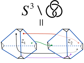
Figure 3: The simplest ideal triangulation of $m004=S^{3}\backslash\mathbf{4_{1}}$.

There are two internal edges in the triangulation which are linearly dependent modulo the linear equations in (29).

$$C_{1}=Z_{1}^{\prime\prime}+Z_{2}^{\prime}+2Z_{1}^{\prime}+2Z_{2}\;,\quad C_{2}=Z_{1}^{\prime\prime}+Z_{2}^{\prime}+2Z_{1}+2Z_{2}^{\prime\prime}\;.$$ (87)

The deformation variety in this example is

$$\begin{split}\mathcal{D}[S^{3}\backslash\mathbf{4_{1}},\mathcal{T}]=&\{z_{1},z_{1}^{\prime},z_{1}^{\prime\prime},z_{2},z_{2}^{\prime},z_{2}^{\prime\prime}:z_{i}^{-1}+z_{i}^{\prime\prime}-1=0,\;z_{i}z_{i}^{\prime}z_{i}^{\prime\prime}=-1,\;z_{1}^{\prime\prime}(z_{1}^{\prime})^{2}z_{2}^{\prime}z_{2}^{2}=1\}_{i=1,2}\;.\end{split}$$ (88)

Each point in the variety gives a $PSL(2,\mathbb{C})=SL(2,\mathbb{C})/\langle\pm 1\rangle$ flat connection on the knot complement. The holonomy matrices along the basis ($\alpha,\beta,\gamma$) of $\pi_{1}(S^{3}\backslash\mathbf{4_{1}})$ for the flat connections is

$$\begin{split}&\rho_{\rm hol}(\alpha)=\left(\begin{array}[]{cc}\sqrt{\frac{z_{1}}{z_{2}}}&0\\ \frac{-1+z_{1}}{\sqrt{z_{1}z_{2}}}&\sqrt{\frac{z_{2}}{z_{1}}}\\ \end{array}\right)\;,\\ &\rho_{\rm hol}(\beta)=\left(\begin{array}[]{cc}\sqrt{\frac{z_{2}^{\prime}}{z_{1}^{\prime\prime}}}&-\sqrt{\frac{z_{2}^{\prime}}{z_{1}^{\prime\prime}}}\\ \sqrt{z_{1}^{\prime\prime}z_{2}^{\prime}}&\,-\sqrt{\frac{z_{1}^{\prime\prime}}{z_{2}^{\prime}}}\left(z_{2}^{\prime}-1\right)\\ \end{array}\right)\;,\\ &\rho_{\rm hol}(\gamma)=\left(\begin{array}[]{cc}\frac{z_{1}^{\prime}+z_{2}^{\prime\prime}-1}{\sqrt{z_{1}^{\prime}z_{2}^{\prime\prime}}}&\frac{1-z_{1}^{\prime}}{\sqrt{z_{1}^{\prime}z_{2}^{\prime\prime}}}\\ \frac{z_{2}^{\prime\prime}-1}{\sqrt{z_{1}^{\prime}z_{2}^{\prime\prime}}}&\frac{1}{\sqrt{z_{1}^{\prime}z_{2}^{\prime\prime}}}\\ \end{array}\right)\;.\end{split}$$ (89)

Boundary (meridian, longitudinal) holonomies are

$$\begin{split}&\rho_{\rm hol}(\mu)={\rm Hol}(\alpha)=\left(\begin{array}[]{cc}e^{a_{\mu}/2}&0\\ &e^{-a_{\mu}/2}\end{array}\right)\;,\quad a(\mu)=Z_{1}-Z_{2}\;,\\ &\rho_{\rm hol}(\nu)={\rm Hol}(\alpha\gamma^{-1}\beta\gamma\alpha^{-1}\beta^{-1})=\left(\begin{array}[]{cc}e^{b_{\lambda}/2}&0\\ &e^{-b_{\lambda}/2}\end{array}\right)\;,\quad b_{\lambda}=2(Z_{1}-Z_{1}^{\prime})\;.\end{split}$$ (90)

So, $(\mu,\lambda)$ is of $(SO(3),SU(2))$ type and we choose

$$X_{\mu}=a_{\mu}=Z_{1}-Z_{2}\;,\quad P_{\lambda}=b_{\lambda}/2=Z_{1}-Z_{1}^{\prime}\;.$$ (91)

With the choices, the $Sp(4,\mathbb{Z})$ matrix $g_{m004}$ in (59) is given by

$$g_{m004}=\left(\begin{array}[]{cccc}1&-1&0&0\\ -2&1&-1&-1\\ 2&0&1&0\\ 0&1&0&0\\ \end{array}\right)\;,$$ (96)

which can be decomposed into $g_{m004}=g^{s}_{J_{m004}}g^{t}_{K_{m004}}g^{gl}_{U_{m004}}$ with (68)

$$U_{m004}=\left(\begin{array}[]{cc}1&-1\\ 0&1\\ \end{array}\right)\;,\quad K_{m004}=\left(\begin{array}[]{cc}2&2\\ 2&1\\ \end{array}\right)\;,\quad J_{m004}=\left(\begin{array}[]{cc}0&0\\ 0&1\\ \end{array}\right)\;.$$ (103)

Following each steps in eq. (61),(70) and (72), $T^{DGG}[m004,X_{\mu};P_{\lambda}]$ is given by

$$\begin{split}&\mathcal{L}_{T_{\rm step1}}(V_{1},V_{2})=\mathcal{L}_{T^{\otimes 2}_{\Delta}}\\ &=\frac{1}{4\pi}\int d^{4}\theta(-\frac{1}{2}\Sigma_{1}V_{1}-\frac{1}{2}\Sigma_{2}V_{2})+\int d^{4}\theta(\Phi_{1}^{\dagger}e^{V_{1}}\Phi_{1}+\Phi_{2}^{\dagger}e^{V_{2}}\Phi_{2})\;,\\ &\mathcal{L}_{T^{DGG}[m004,X_{\mu};P_{\lambda}]}(V_{X},V_{C})=\mathcal{L}_{T_{\rm step2}}(V_{X},V_{C})\\ &=\frac{1}{4\pi}\int d^{4}\theta\left(-\frac{1}{2}\Sigma_{C}V_{X}+\Sigma(2V_{C}+3V_{X})\right)+\int d^{4}\theta\left(\Phi_{1}^{\dagger}e^{V+\frac{V_{X}}{2}}\Phi_{1}+\Phi_{2}^{\dagger}e^{V-\frac{V_{X}}{2}}\Phi_{2}\right)\;.\end{split}$$ (104)

Here $V(\textrm{with }\Sigma:=\bar{D}DV)$ is a dynamical $U(1)$ vector multiplet while $V_{X}(\Sigma_{X})$ and $V_{C}(\Sigma_{C})$ are background multiplets coupled to flavor symmetries, $U(1)_{X_{A}}$ and say $u(1)_{C}$ respectively. Note that both of $C_{1}$ and $C_{2}$ are hard internal edges and we can not break the $u(1)_{C}$ associated to them.

Example : $N=S^{3}\backslash\mathbf{4}_{1}=m004$ with an ideal triangulation with 6 tetrahedra

The absence of chiral primary operators corresponding to hard edges in the above construction of $T^{DGG}[m004,X_{\mu};P_{\lambda}]$ using 2 tetrahedra were already noticed in Dimofte:2011ju . The interpretation there was that this is due to the “bad" choice of triangulation, which contains hard internal edges, and can be cured by choosing a proper ideal triangulation which does not have a hard internal edge. As a “good" ideal triangulation for $m004$, they propose the one using six tetrahedra, $\Delta_{R,S,X,Y,Z,W}$ . The internal edges in the triangulation are Dimofte:2011ju

$$\begin{array}[]{ll}C_{1}=X+W+2(R^{\prime}+S^{\prime}+Z^{\prime\prime}),&C_{2}=R+Y+2(Z^{\prime}+W^{\prime}+S^{\prime\prime}),\\ C_{3}=S+W+2(R^{\prime\prime}+X^{\prime\prime}+Y^{\prime}),&C_{4}=R+Z+2(Y^{\prime\prime}+W^{\prime\prime}+X^{\prime}),\\ C_{5}=X+Y,&C_{6}=S+Z.\end{array}$$ (108)

Note that there is no hard internal edges in the triangulation and 5 internal edges are linearly independent. Superficial counting suggests that the resulting theory have a flavor symmetry of rank $6-5=1$, where five $u(1)$s are broken by superpotential operators.

Our interpretation on this problem is different from Dimofte:2011ju . We claim that the theory realized by six tetrahedra is actually completely the same as the one realized by two tetrahedra in the low energy limit. Therefore, the theory constructed by six tetrahedra has a hidden additional $u(1)$ symmetry in the low energy limit which corresponds to the hard edge in the triangulation with two tetrahedra.

To see it, let us focus on the two tetrahedra $\Delta_{X}$ and $\Delta_{Y}$, which are glued in such a way that the system has the internal edge $C_{5}=X+Y$. Then, this theory is described by two chiral fields $\Phi_{X}$ and $\Phi_{Y}$ with the Lagrangian

$$\int d^{4}\theta(\Phi_{X}^{\dagger}\Phi_{X}+\Phi_{Y}^{\dagger}\Phi_{Y})+\int d^{2}\theta\Phi_{X}\Phi_{Y}+{\rm h.c.},$$ (109)

where we have neglected background fields. The superpotential is due to the presence of the internal edge $C_{5}=X+Y$. Then it is clear that these fields $\Phi_{X}$ and $\Phi_{Y}$ can be integrated out and the theory becomes empty in the low energy limit. This means that two tetrahedra $\Delta_{X}$ and $\Delta_{Y}$ are eliminated. Mathematically this corresponds to the 0-2 move. The invariance of a topological quantity called 3d index (see appendix A) under the 0-2 move is proven in 2013arXiv1303.5278G . The definition of the topological quantity is based on ideal triangulation and is equivalent to the localization expression for the superconformal index of $T^{DGG}$ theory. Intuitively, the constraints $0<\mathop{\mathrm{Im}}[X],\mathop{\mathrm{Im}}[Y]<\pi$ and $C_{5}=2\pi i$ mean that $\mathop{\mathrm{Im}}[X],\mathop{\mathrm{Im}}[Y]\to\pi$, and hence these tetrahedra are squashed to be flat. The same comment also applies to $\Delta_{S}$, $\Delta_{Z}$ and $C_{6}=S+Z$.

At the level of edge variables, the process of integrating out the massive fields may be done by eliminating the variables corresponding to the massive fields. More explicitly, we define

$$C^{\prime}_{1}:=C_{3}+C_{4}+2C_{5}-C_{6}-4\pi i=W+R+2W^{\prime\prime}+2R^{\prime\prime}$$ (110)

$$C^{\prime}_{2}:=C_{1}+C_{2}-C_{5}+2C_{6}-4\pi i=W+R+2W^{\prime}+2R^{\prime},$$ (111)

After renaming $W\to Z_{1}^{\prime\prime},~{}R\to Z_{2}^{\prime}$ and so on, these variables $C^{\prime}_{1}$ and $C^{\prime}_{2}$ become the same as the ones in the triangulation with two tetrahedra.

2.3 Relation between the two constructions

One basic characteristic of the $T^{DGG}[N,X_{A}]$ theory is that Dimofte:2011ju

$$\begin{split}&\mathcal{M}_{\rm parameter}(\textrm{$T^{DGG}[N,X_{A}]$ on $\mathbb{R}^{2}\times S^{1}$})=\mathcal{D}[N,\mathcal{T}]\supseteq\chi_{0}(N)\;.\end{split}$$ (112)

Recall the definition of each term of this equation. For simplicity, we only discuss the case where our 3-manifold $N$ only has a torus boundary and hence of the form $N=M\backslash K$. The deformation variety $\mathcal{D}[N,\mathcal{T}]$ defined in (32) is a set of flat $PSL(2,\mathbb{C})$ connections on $N$ which can be obtained from an ideal triangulation $\mathcal{T}$. The $\chi_{0}(N)$ is a subset of the algebraic variety defined in (24) (or (35)) which can be seen for any non-exotic ideal triangulation. The difference between the two sets are mild, higher codimension, and may be ignorable in our discussion as we discuss later. Finally the left-hand side $\mathcal{M}_{\rm parameter}(\textrm{$T^{DGG}[N,X_{A}]$ on $\mathbb{R}^{2}\times S^{1}$})$ is given as follows. A DGG theory in general consists of chiral fields, dynamical vector fields, and background vector fields. Let $\Sigma_{i}~{}(i=1,\ldots,N_{V})$ be twisted chiral fields constructed from dynamical vector multiplets whose lowest real component is the real scalar of the vector multiplet and the imaginary part is the gauge field in the $S^{1}$ direction. The $N_{V}$ is the number of dynamical vector multiplets, i.e., the gauge group is $u(1)^{N_{V}}$, and it depends on the details of $g_{N}$ in (70) and its decomposition into basic types. Also, let $X_{A}$ be the twisted chiral field of the background $u(1)$ field whose real part corresponds to the real mass parameter $m$ and the imaginary part corresponds to the background flavor gauge field around $S^{1}$. Then, by integrating out the matter chiral fields of the theory on ${\mathbb{R}}^{2}\times S^{1}$, we get a twisted superpotential of $\Sigma_{i}$ and $X_{A}$ (in some appropriate normalization),

$$\widetilde{\mathcal{W}}(\{\Sigma_{i}\}_{i=1}^{N_{V}};X_{A}).$$ (113)

Then we define

$$\begin{split}&\mathcal{M}_{\rm parameter}(\textrm{$T^{DGG}[N,X_{A}]$ on $\mathbb{R}^{2}\times S^{1}$})\\ &=\big{\{}(e^{X_{A}},e^{P_{B}}):\exp\big{(}\partial_{\Sigma_{k}}\widetilde{\mathcal{W}}(\{\Sigma_{i}\}_{i=1}^{N_{V}};X_{A})\big{)}=1,\partial_{X_{A}}\widetilde{\mathcal{W}}(\{\Sigma_{i}\}_{i=1}^{N_{V}};X_{A})\big{)}=P_{B}\big{\}}\backslash\{\textrm{singular loci}\}.\end{split}$$ (114)

The conditions $\exp\big{(}\partial_{\Sigma_{k}}\widetilde{\mathcal{W}}(\{\Sigma_{i}\}_{i=1}^{N_{V}};X_{A})\big{)}=1$ are just the condition for the vacua on $S^{1}\times{\mathbb{R}}^{2}$. The $P_{B}$ has a definite value (modulo $2\pi i$) at each of the vacua for a given parameter $X_{A}$. In other words, the equation $\partial_{X_{A}}\widetilde{\mathcal{W}}(\{\Sigma_{i}\}_{i=1}^{N_{V}};X_{A})\big{)}=P_{B}$ gives a polynomial equation of $(x_{A},p_{B}):=(e^{X_{A}},e^{P_{B}})$, and solutions of that equation in terms of $p_{B}$ for a given $x_{A}$ correspond to the vacua of the theory with mass parameter $x_{A}$.

The relation to localization computation is as follows. The partition function of the $T^{DGG}$ theory on a curved background called squashed 3-sphere $(S^{3}_{b})$ can be written in following form Hama:2011ea ; Dimofte:2011ju

$$\int d\sigma_{1}\ldots d\sigma_{N_{V}}\;\mathcal{I}_{b}(\{\sigma_{i}\}_{i=1}^{N_{V}};X_{A})$$ (115)

where $\sigma_{k}=\mathop{\mathrm{Re}}[\Sigma_{k}]$. In a degenerate limit when $b\rightarrow 0$, which corresponds to the limit where $S^{3}_{b}$ become $\mathbb{R}^{2}\times S^{1}$, the leading asymptotic behavior of the integrand is determined by the twisted superpotential

$$\mathcal{I}_{b}(\{\sigma_{i}\}_{i=1}^{N_{V}};X_{A})\xrightarrow[]{\quad b\rightarrow 0\quad}e^{\frac{1}{2\pi ib^{2}}\widetilde{\mathcal{W}}(\{\sigma_{i}\}_{i=1}^{N_{V}};X_{A})}\;.$$ (116)

The equations $\{\exp(\partial_{\Sigma_{i}}\widetilde{\mathcal{W}})=1\}_{i=1}^{N_{V}}$ are equivalent to the gluing equations in (32) with an additional relation $e^{a}=(-1)^{\epsilon}\prod z_{i}^{\alpha_{i}}(1-z_{i}^{-1})^{\alpha^{\prime\prime}_{i}}$ where $a=X_{A}~{}\text{or}~{}2X_{A}$ depending on $SO(3)/SU(2)$ types of boundary cycle $A$, and the integers $(\alpha_{i},\alpha^{\prime\prime}_{i},\epsilon)$ are given in (34) Dimofte:2012qj .

Now, we have

$$\mathcal{M}_{\rm vacua}(\textrm{$T^{DGG}[N,X_{A}]$ on $\mathbb{R}^{2}\times S^{1}$})$$

$$= \mathcal{M}_{\rm parameter}(\textrm{$T^{DGG}[N,X_{A}]$ on $\mathbb{R}^{2}\times S^{1}$})|_{a=2m}.$$ (117)

This means that by taking the parameter $a$ to be a constant fixed value $2m$, we get the vacua of the theory with the mass parameter $m$.

The above equations may have solutions like $X_{A}=0$. Field theoretically, when the mass parameter is zero, there could appear some continuous moduli space of vacua spanned by matter chiral fields. Those massless flat directions are subtle, especially when they are generated by monopole operators because in that case those directions appear by very strong coupling effects which may not be captured by the one-loop computation of the twisted superpotential $\widetilde{\mathcal{W}}$. See Sec. 5.2 of Dimofte:2011ju for an example. We may expect that those subtle flat directions might be the reason of the mismatch between $\mathcal{D}[N,\mathcal{T}]$ and $\chi_{0}(N)$ This problem may be avoided if we only consider generic mass parameters. We assume that this is the case.

Comparison of the two constructions

Now let us compare the constructions in Sec. 2.1 and Sec. 2.2. Comparing the moduli space of $T^{6d}$ in (19), and $T^{DGG}$ in (117) we see that

$$\mathcal{M}_{\rm vacua}(\textrm{$T^{DGG}[N,X_{A}]$ on $\mathbb{R}^{2}\times S^{1}$})\subset\mathcal{M}_{\rm vacua}(\textrm{$T^{6d}[N,A]$ on $\mathbb{R}^{2}\times S^{1}$})\;.$$ (118)

This is because that an ideal triangulation captures only a subset of irreducible flat connections on $N$ as emphasized in Chung:2014qpa . So we see that $T^{DGG}$ can not be identical to $T^{6d}$ but can only capture a subsector of $T^{6d}$. This point has already been seen from the effective field theory point of view in Sec. 2.1. In general, there is no reason to expect that there exists a genuine 3d theory which describes all components of moduli space of vacua of $T^{6d}$. So $T^{DGG}$ can, at best, describe the low energy limit of some point of the moduli space of vacua of $T^{6d}$.

Then a possibility is that $T^{DGG}$ might be identified with $T^{6d}_{\rm irred}$ in (10). Both of them are genuine 3d theories and they are associated to the hyperbolic connection ${\cal A}^{\rm\overline{hyp}}$ which can be realized in ideal triangulation. However, it turns out that these two theories are still different as we now explain.

One crucial difference between the two theories is that $T^{DGG}$ generically has $U(1)_{X_{A}}$ flavor symmetry associated to the knot while $T^{6d}$ and hence $T^{6d}_{\rm irred}$ have $su(2)_{A}$. Furthermore, the $SL(2,\mathbb{Z})$ action on the canonical variables $(X_{A},P_{B})$ is realized in field theory as the $SL(2,\mathbb{Z})$ action of Witten Witten:2003ya using $u(1)$ group on $T^{DGG}$, while the $SL(2,\mathbb{Z})$ action on the boundary cycle $(A,B)$ is realized in field theory as the $SL(2,\mathbb{Z})$ of Gaiotto-Witten Gaiotto:2008ak using the $su(2)$ symmetry and $T[SU(2)]$ theory on $T^{6d}$.

The $su(2)$ $SL(2,\mathbb{Z})$ on $T^{6d}$ is defined as follows. The transformed theory $\varphi\cdot T^{6d}[N,A,B]$ with

$$\varphi=\left(\begin{array}[]{cc}r&s\\ p&q\end{array}\right)\;\in SL(2,\mathbb{Z})$$ (121)

can be obtained by

$$\begin{split}&T^{6d}[N,rA+sB;pA+qB]=\varphi\cdot T^{6d}[N,A;B]\\ &:=\textrm{coupling the duality wall theory $T[SU(2),\varphi]$ to $T^{6d}[N,A;B]$ }\;.\end{split}$$ (122)

$T[SU(2),\varphi]$ is a 3d $\mathcal{N}=4$ SCFT which describe the 3d theory living on a duality domain wall in 4d $su(2)$ $\mathcal{N}=4$ SYM associated to $\varphi\in SL(2,\mathbb{Z})$. The theory has $su(2)_{1}\times su(2)_{2}$ as flavor symmetry. For example, $T[SU(2),\varphi=S]=T[SU(2)]$. In the coupling between $T[SU(2),\varphi]$ and $T^{6d}[N,A;B]$, we introduce a $\mathcal{N}=2$ vector multiplet to gauge the diagonal $su(2)_{\rm diag}\subset su(2)_{1}\times su(2)_{A}$ of the two theories with the following superpotential coupling

$$\textrm{Tr}(\mu\mu^{\prime})\;.$$ (123)

where $\mu$ is the holomorphic moment map operator associated to the $su(2)_{A}$ of $T^{6d}[N,A;B]$ which is a chiral operator in the adjoint representation of $su(2)_{A}$, and $\mu^{\prime}$ is the holomorphic moment map operator of $su(2)_{1}$ of $T[SU(2),\varphi]$.

Motivated by the similarities and differences between $T_{\rm irred}^{6d}$ and $T^{DGG}$, we propose the following relation between them:

$$T^{6d}\xrightarrow[\text{}]{\textrm{\quad on a vacuum $P_{\rm SCFT}$}\quad}T^{6d}_{\rm irred}\xrightarrow[\text{}]{\textrm{\quad deformed by $\delta W=\mu^{3}$}\quad}T^{DGG}$$ (124)

Here, $\mu^{3}$ is the Cartan component of the moment map operator ${\mu}=\{\mu^{1},\mu^{2},\mu^{3}\}$ in the adjoint representation of $su(2)_{A}$. The $\delta W=\mu^{3}$ means the superpotential deformation by the chiral operator $\mu^{3}$. This deformation breaks $su(2)$ to $U(1)$.

Thus we need two steps from $T^{6d}$ to $T^{DGG}$. First we put the theory on a specific vacuum, $P_{\rm SCFT}$, of the $T^{6d}$ theory on $\mathbb{R}^{3}$ as explained in Sec. 2.1. As a second step, we deform the intermediate theory, $T^{6d}_{\rm irred}$, by adding the Cartan component ($\mu^{3}$) of the $su(2)$ moment map operator $\mu$ associated to the knot to the superpotential. We give more evidence for this proposal below.

In the case of 3d ${\cal N}=4$ supersymmetry, the presence of the holomorphic moment map operator associated to a symmetry is guaranteed. However, when there are only ${\cal N}=2$, it is not guaranteed. What we call the holomorphic moment map operator is a kind of remnant of higher supersymmetry of the codimension-2 defect of the 6d ${\cal N}=(2,0)$ theory. The $\mu$ may be empty depending on the theory. However, generically (but not always), the $T^{6d}_{\rm irred}$ theory contains the moment map as chiral operators. This can be seen as follows. Suppose we are given a theory ${\cal T}$ with $su(2)$ symmetry, and then let us perform a transformation

$$ST^{k}\in SL(2,{\mathbb{Z}})$$ (125)

acting on this $su(2)$. This is done by coupling ${\cal T}$ and $T[SU(2)]$ to the $su(2)$ gauge field with Chern-Simons level $k(+\text{ the original value before }T^{k})$. By taking $k$ large enough, the $su(2)$ gauge field is weakly coupled and hence the two theories ${\cal T}$ and $T[SU(2)]$ almost decouple from each other. The $T[SU(2)]$ theory contains the holomorphic moment map operator $\mu$ associated to the new (ungauged) $su(2)$ global symmetry. Therefore, we conclude that the total theory has $\mu$ for generic $k$. Moreover, this argument shows that the scaling dimension of $\mu$ is close to 1, at least if $k$ is large enough, because the scaling dimension of $\mu$ in $T[SU(2)]$ alone is 1 by ${\cal N}=4$ supersymmetry. Therefore, the deformation by $\mu^{3}$ is a relevant deformation and it triggers RG flows. The case that $\mu$ is absent happens only in rather exceptional situations, and this will be very important in Sec. 3

In particular, the deformation breaks the $su(2)_{A}$ in $T_{\rm irred}^{6d}[N,A]$ to $U(1)$ which can be identified with $U(1)_{X_{A}}$ in $T^{DGG}[N,X_{A}]$.

$$\big{(}su(2)_{A}\textrm{ of $T^{6d}_{\rm irred}$}\big{)}\;\xrightarrow[\text{}]{\quad\delta W=\mu^{3}\quad}\;\big{(}U(1)_{X_{A}}\textrm{ of $T^{DGG}$}\big{)}\;.$$ (126)

More details on $SL(2,{\mathbb{Z}})$ transformations of $U(1)$ and $SU(2)/SO(3)$ types.

The deformation explains not only why $T^{DGG}$ theory generically has only $U(1)_{X_{A}}$ associated to the knot, but also why the $SL(2,\mathbb{Z})$ action on the boundary $\mathbb{T}^{2}$ of the knot complement corresponds to the $U(1)$ $SL(2,\mathbb{Z})$ action on $U(1)_{X_{A}}$. Roughly, the relation is given by the following diagram;

(131)

However, there are more subtle details.

We denote the $U(1)$-type and $su(2)$-type $SL(2,{\mathbb{Z}})$ transformations as $SL(2,{\mathbb{Z}})_{1}$ and $SL(2,{\mathbb{Z}})_{2}$, respectively. The $SL(2,{\mathbb{Z}})_{1}$ acts on the canonical variables $(X_{A},P_{B})$, while $SL(2,{\mathbb{Z}})_{2}$ acts on $(A,B)$ and hence on the variables $(a,b)$. Recall that they are related as

$$(X_{A},P_{B})=\begin{cases}(\frac{a}{2},b)\;,\;\textrm{when $(A,B)$ is of $\big{(}SU(2),SO(3)\big{)}$ type}\\ (a,\frac{b}{2})\;,\;\textrm{when $(A,B)$ is of $\big{(}SO(3),SU(2)\big{)}$ type}\end{cases}$$ (132)

Therefore, generic elements of $SL(2,{\mathbb{Z}})_{1}$ and $SL(2,{\mathbb{Z}})_{2}$ do not exactly correspond to each other.

The $S$-transformation $S_{1}\in SL(2,{\mathbb{Z}})_{1}$ and $S_{2}\in SL(2,{\mathbb{Z}})_{2}$ correspond with each other;

$$S_{1} :(X_{A},P_{B})\to(-P_{B},X_{A})$$

$$S_{2} :(a,b)\to(-b,a)$$ (133)

and hence

$$S_{1}\longleftrightarrow S_{2}.$$ (134)

Notice that the $S_{2}$ exchanges the $SU(2)/SO(3)$ types of the cycles. This is natural, because in 4d ${\cal N}=4$ theory, the gauge groups $SU(2)$ and $SO(3)$ are exchanged under the S-duality. This exchange can also be shown in purely 3d language and is explained in Appendix B.

On the other hand, the $T$-transformation $T_{1}\in SL(2,{\mathbb{Z}})_{1}$ and $T_{2}\in SL(2,{\mathbb{Z}})_{2}$ act as

$$T_{1} :(X_{A},P_{B})\to(X_{A},P_{B}+X_{A})$$

$$T_{2} :(a,b)\to(a,b+a)$$ (135)

and hence they are related as

$$(T_{1})^{2}\leftrightarrow T_{2}\qquad\textrm{when $(A,B)$ is of $\big{(}SU(2),SO(3)\big{)}$ type}$$ (136)

$$T_{1}\leftrightarrow(T_{2})^{2}\qquad\textrm{when $(A,B)$ is of $\big{(}SO(3),SU(2)\big{)}$ type}$$ (137)

This also has a natural field theory interpretation. Let $A$ be an $su(2)$ gauge field. The global structure may be either $SU(2)$ or $SO(3)$. Its Chern-Simons 3-form is defined as

$${\rm CS}(A)=\frac{1}{4\pi}\operatorname{tr}(AdA+\frac{2}{3}A^{3}),$$ (138)

where the trace is taken in the doublet representation of $su(2)$. When the symmetry is $SU(2)$ and is broken down to $U(1)$, we embed a $U(1)$ gauge field $a$ inside $A$ as $A=\mathop{\rm diag}\nolimits(a,-a)$. Then, under this embedding, we get

$${\rm CS}(A)\to\frac{2}{4\pi}ada=2{\rm CS}(a)$$ (139)

where

$${\rm CS}(a)=\frac{1}{4\pi}ada.$$ (140)

Recalling that the $T$-transformation in field theory corresponds to the shift of Chern-Simions level of background field, we can see that the factor of 2 in (139) corresponds to the exponent 2 in (136). In the same way, if the gauge group is $SO(3)$ which is broken to $U(1)$, it is natural to embed the $U(1)$ gauge field as $A=\frac{1}{2}(a,-a)$. Then we get

$${\rm CS}(A)\to\frac{1}{2\cdot 4\pi}ada=\frac{1}{2}{\rm CS}(a).$$ (141)

This equation corresponds to (137).

In fact, if the group is $SO(3)$ type, then the ${\rm CS}(A)$ is not a properly quantized Chern-Simons invariant. This is because, in 4d, there can be instantons of instanton number $1/2$, and hence the integral of ${\rm CS}(A)$ is not well defined in 3d, and only the $2{\rm CS}(A)$ is well defined. This means that when the $A$-cycle is $SO(3)$ type, only the $(T_{2})^{2}$ is well defined. Therefore, the actual transformation group at the quantum level is a subgroup $\Gamma(2)\subset SL(2,{\mathbb{Z}})_{2}$ generated by $S_{1}$ and $(T_{2})^{2}$. These generators $S_{1}$ and $(T_{2})^{2}$ also preserves the condition that one of the cycles $A$ or $B$ is $SU(2)$ type. Under $T_{2}$, this condition may not be preserved.

From the above discussion of Chern-Simons levels, the field theoretical realization of (136) and (137) under the explicit breaking $su(2)_{A}\to U(1)_{X_{A}}$ by $W=\mu^{3}$ is clear. Now let us also check the correspondence of the S-transformation (134) at the field theory level. Let ${\cal T}$ be a theory with $su(2)$ symmetry. Then $S$-transformed theory is given by

$$S_{2}\cdot{\cal T}={\cal T}-su(2)-T[SU(2)],$$ (142)

where the center $su(2)$ is a gauge group which is coupled to the $su(2)$ symmetry of ${\cal T}$ and the $su(2)_{H}$ symmetry of $T[SU(2)]$. In the language of 3d ${\cal N}=2$ supersymmetry, the $T[SU(2)]$ is given by a $U(1)$ vector multiplet $V$, a neutral chiral field $\phi$, and two pairs of chiral fields $(E^{i},\tilde{E}_{i})_{i=1,2}$ with $u(1)_{\rm gauge}$ charge $\pm$ with the superpontial

$$W=\phi\tilde{E}_{i}E^{i}.$$ (143)

The $su(2)_{H}$ acts on the index $i$ of $(E^{i},\tilde{E}_{i})_{i=1,2}$. Now, this $T[SU(2)]$ has a $su(2)_{C}$ symmetry at the quantum level, and this symmetry is the new global $su(2)$ symmetry after the $S$-transformation. See Appendix B for more details. The Cartan component $\mu^{3}$ of the moment map operator of this symmetry $su(2)_{C}$ is given by $\mu^{3}=\phi$. Therefore, after the deformation by $\mu^{3}$, the superpotential becomes

$$W=\phi\tilde{E}_{i}E^{i}-\phi.$$ (144)

Thus, an F-term condition is $\tilde{E}_{i}E^{i}=1$. Then $\tilde{E}_{i}$ and $E^{i}$ get nonzero expectation values as

$$\langle E^{1}\rangle=\langle\tilde{E}_{1}\rangle=1,~{}~{}~{}\langle E^{2}\rangle=\langle\tilde{E}_{2}\rangle=0.$$ (145)

These expectation values break the gauge symmetry $[su(2)\times u(1)]_{\rm gauge}$ down to $u(1)$. Namely, $(E^{i},\tilde{E}_{i})$ are charged under $u(2)=[su(2)\times u(1)]_{\rm gauge}$, and only the subgroup $u(1)\subset u(2)$ which acts on $(E^{2},\tilde{E}_{2})$ is preserved by the expectation values. Therefore, by the Higgs mechanism, the theory (142) becomes

$$S_{2}\cdot{\cal T}\longrightarrow S_{1}\cdot{\cal T}={\cal T}-u(1),$$ (146)

where $u(1)$ is the gauge group which survives the symmetry breaking $[su(2)\times u(1)]_{\rm gauge}\to u(1)$. The right hand side is just the $S$-transformation of $u(1)$ type. This confirms (134).

3 Symmetry enhancement

Using the proposed 6d interpretation of $T^{DGG}[N,X_{A}]$ in (124), we will determine the symmetry enhancement pattern of the $U(1)_{X_{A}}$ symmetry associated to the knot based on a topological type of the boundary cycle $A$. See the Table 1 for the summary whose details will be explained in Sec. 3.1.

$A\in H_{1}\big{(}\partial N,\mathbb{Z}\big{)}$	Symmetry enhancement of $U(1)_{X_{A}}$ in $T^{DGG}[N,X_{A}]$
closable	$U(1)_{X_{A}}\rightarrow U(1)$
non-closable, $SO(3)$ type	$U(1)_{X_{A}}\rightarrow SO(3)$
non-closable, $SU(2)$ type	$U(1)_{X_{A}}\rightarrow SU(2)$

Table 1: Symmetry enhancement in $T^{DGG}[N,X_{A}]$. The definitions of “$SU(2)/SO(3)$ types” are explained in Sec. 2.2. The definitions of “closable/non-closable” are explained in Sec. 3.1.

In Sec. 3.2, we will find infinitely many examples of pair $(N,A)$ and $(N^{\prime},A^{\prime})$ whose corresponding DGG theories are identical and both of $A$ and $A^{\prime}$ are non-closable but one of them (say $A$) is $SO(3)$ type while the other ($A^{\prime}$) is $SU(2)$ type. In that case, combining the table 1 with a group theoretical argument, we can argue that the DGG theory has enhanced $SU(3)$ symmetry. Using the argument, we prove that $T^{DGG}[M=S^{3},K]$ theories for all hyperbolic twist knots $K$ have $SU(3)$-symmetry. We checked the enhancement for several twist knots which gives non-trivial empirical evidence for the Table 1.

3.1 $SO(3)/SU(2)$ enhancement

From the relation between $T_{\rm irred}^{6d}$ and $T^{DGG}$ in (124), we understand the symmetry breaking mechanism of $su(2)_{A}$ to $U(1)_{X_{A}}$. For the symmetry breaking to happen, we need the $su(2)$ moment map operator $\mu$ in $T^{6d}_{\rm irred}$ theory. Otherwise, the $su(2)_{A}$ is not broken by the mechanism and the resulting $T^{DGG}$ is expected to have an $su(2)$ symmetry. Therefore, we need to know when $\mu$ is absent.

This question can be answered by an inspection of the 5d picture discussed in Sec. 2.1. In the description there, the moment map operator comes from the holomorphic $su(2)_{C}$ moment map of $T[SU(2)]$ theory which is put along a knot $K$. After $S^{1}$ compactification, the $T[SU(2)]$ has 2d ${\cal N}=(4,4)$ supersymmetry. In the Language of ${\cal N}=(2,2)$ supersymmetry, there is a twisted chiral operator $\widetilde{\mu}$ and a chiral operator $\mu$, both of which are associated to the Coulomb branch $su(2)_{C}$ symmetry of $T[SU(2)]$.

Now suppose that the Higgs branch operator $\widetilde{\nu}$ gets a nonzero expectation value. Then, the nonzero VEV in Higgs branch makes the Coulomb branch fields massive. Therefore, in the low energy limit, the operators $\mu$ and $\widetilde{\mu}$ become empty;

In $$T[SU(2)] \langle\tilde{\nu}\rangle\neq 0 \mu$$ theory on , is absent at low-energy (147)

In the coupled system (5d SYM+ $T[SU(2)]$), as shown in (20), the VEV of the moment operator $\widetilde{\nu}$ is given by $\log\rho_{\rm hol}(A)$ of complexified gauge field $\mathcal{A}$. The $\mathcal{A}$ is a flat connection in $\chi_{0}[N]$ defined in (24) and (35). Thus the above relation implies that the $T^{6d}_{\rm irred}$ theory on $\mathbb{R}^{2}\times S^{1}$ does not contain $\mu$ if there is no $PSL(2,\mathbb{C})$ flat-connection in $\chi_{0}[N]$ with trivial $\rho_{\rm hol}({\cal A})$. Let us define

$$\begin{split}&\textrm{A primitive boundary cycle $A\in H_{1}(\partial N,\mathbb{Z})$ is `closable'}\\ &\textrm{if there is a point in $\chi_{0}[N]$ with $\rho_{\rm hol}(A)=1$\;.}\end{split}$$ (148)

We remark that in the massless case $m=0$, the eigenvalues of $\rho_{\rm hol}(A)$ are trivial ($\pm 1$), but $\rho_{\rm hol}(A)$ may contain off-diagonal components and hence the above condition is nontrivial. Then,

$$\begin{split}&\textrm{$A\in H_{1}(\partial N,\mathbb{Z})$ is non-closable }\\ &\Rightarrow\;\textrm{$\mu$ is absent in $T^{6d}_{\rm irred}[N,A]$ on $\mathbb{R}^{2}\times S^{1}$ for any radius of $S^{1}$ at low energy}\\ &\Rightarrow\;\textrm{$\mu$ is absent in $T^{6d}_{\rm irred}[N,A]$ on $\mathbb{R}^{3}$ at low energy }\\ &\Rightarrow\;T^{DGG}[N,X_{A}]=T^{6d}_{\rm irred}[N,A]\textrm{ has $su(2)$ symmetry at low energy}\;.\end{split}$$ (149)

Strictly speaking, the step from ${\mathbb{R}}^{2}\times S^{1}$ to ${\mathbb{R}}^{3}$ is nontrivial, but we assume that this step holds.

One necessary condition for $A$ to be ‘non-closable’ is that the Dehn filled manifold $N_{A}$ is non-hyperbolic.

$$\textrm{If $N_{A}$ is hyperbolic}\;\Rightarrow\;\textrm{$A$ is closable}\;.$$ (150)

This is because that the flat connection corresponding to the hyperbolic structure on $N_{A}$ is always contained in $\chi_{0}[N]$ with trivial $\rho_{\rm hol}(A)$. According to Thurston’s hyperbolic Dehn surgery theorem, for given hyperbolic $N$, there are only finite number of primitive boundary cycles $A$ which give non-hyperbolic $N_{A}$. So, we can conclude that

$$|\{\textrm{Set of primitive `non-closable' boundary cycles $A\in H_{1}(\partial N,\mathbb{Z})$}\}|<\infty\;.$$ (151)

Combining with Table 1, it implies that the $u(1)_{X_{A}}$ symmetry of $T^{DGG}[N,X_{A}]$ is not enhanced to $su(2)$ except for only finite many $A$s. The Thurston’s theorem is consistent with our field theoretical consideration in the previous section that the moment map operator $\mu$ generically (although not always) exists; see the discussion in the paragraph containing (125).

One sufficient condition for $A$ to be ‘non-closable’ is that the Dehn filled manifold $N_{A}$ is Lens-space

$$\textrm{If $N_{A}$ is Lens space}\;\Rightarrow\;\textrm{$A$ is non-closable}\;.$$ (152)

Lens space $L(p,q)$ is defined as

$$L(p,q):=\big{(}S^{3}\backslash(\textrm{unknot})\big{)}_{p\mu+q\lambda}$$ (153)

The reason is as follows. If $A$ is closable, by definition, there should be an irreducible flat connection in $\chi_{0}[N]$ with trivial $\rho_{\rm hol}(A)$. Such a flat connection can be thought as an irreducible flat connection on $N_{A}$. But if $N_{A}$ is a Lens space, there can not be any irreducible flat connection because the fundamental group $\pi_{1}$ of Lens space is abelian. Thus the cycle $A$ can not be closable. When $N_{A}$ is neither hyperbolic nor a Lens space, no simple criterion to determine the closability has been found.

An alternative definition of closable/non-closable cycle, which seems to be equivalent to the above definition, is using 3d index which is introduced in Dimofte:2011py as a topological invariant of 3-manifolds with torus boundaries and is generalized in Appendix A to cover closed 3-manifolds.

$$\begin{split}&\textrm{A primitive boundary cycle $A\in H_{1}(\partial N,\mathbb{Z})$ is closable (non-closable)}\\ &\textrm{if $\mathcal{I}_{N_{A}}(x)\neq 0$\;($\mathcal{I}_{N_{A}}(x)=0$)\;.}\end{split}$$ (154)

Here $\mathcal{I}_{N_{A}}(x)$ is the 3d index on a closed 3-manifold $N_{A}$. That a primitive boundary cycle $A\in H_{1}(\partial N,\mathbb{Z})$ is ‘non-closable’ means that we can not ‘close’ (or eliminate) the co-dimension two defect along a $K$ on $M$ in a supersymmetric way after sitting on the vacuum $P_{\rm SCFT}$. As we will study in the next section, there is an operation in SCFT side of 3d/3d correspondence which corresponds to the operation of ‘closing the knot’. If $A$ is non-closable cycle, we expect that the resulting 3d theory $T^{6d}_{\rm irred}[M]$ after taking the closing knot operation on $T^{6d}_{\rm irred}[M,K]$ will be a theory with supersymmetry broken. The index $\mathcal{I}_{M=N_{A}}(x)$ computes the superconformal index of the theory $T^{6d}_{\rm irred}[M]$ and expected to be zero when $A$ is non-closable and thus supersymmetry is broken. This is a heuristic argument supporting the equivalence between the two definitions and no rigorous mathematical proof is known. We checked the equivalence for various examples and the equivalence seems to hold possibly except for exotic cases. As an example, see Table 2 for the case when $N=S^{3}\backslash\mathbf{4_{1}}=m004$.

$A\in H_{1}(\partial N,\mathbb{Z})$	Closability	$\mathcal{I}_{N_{A}}(x)$
$p\mu+\lambda\;(|p|\geq 5)$	closable ($\Leftarrow$ $N_{A}$ is hyperbolic)	non-trivial power series in $x$
$p\mu+\lambda\;(|p|=4)$	closable	divergent
$p\mu+\lambda\;(|p|<4)$	closable	1
$\mu$	non-closable	0

Table 2: Closability of boundary cycles of $N=S^{3}\backslash\mathbf{4_{1}}$. The $\mu$ is meridian and $\lambda$ is longitude. We determine the closability using the definition in (148) and the $\mathcal{D}[N,\mathcal{T}]$ in (88) with (89) and (90)

We can further determine the global structure of enhanced symmetry, whether $SO(3)$ or $SU(2)$, from the $SO(3)/SU(2)$ type of $A$. When $A$ is non-closable and of $SU(2)$ type, the compact $U(1)_{X_{A}}$ symmetry of $T^{DGG}[N,X_{A}]$ is embedded into the enhanced $su(2)_{A}$ symmetry via $\mathbf{2}_{su(2)_{A}}\rightarrow(\pm 1)_{U(1)_{X_{A}}}$. This is manifest from the relations given in eq. (34) and (60) between the variable $X_{A}$, associated to the $U(1)_{X_{A}}$, and the $PSL(2,\mathbb{C})$ holonomy variables $a$, associated to the $su(2)_{A}$. Namely, $\mathbf{2}_{su(2)}$ has properly quantized $U(1)_{X_{A}}$ charges and the theory can have operators charged under half integer spin representations of $su(2)_{A}$ which means that the symmetry is $SU(2)$. Similarly we can see that only operators in integer spin representation are allowed when $A$ is of $SO(3)$ type. See also Appendix B for more justifications from different arguments.

In general, it is not easy to determine the $SO(3)/SU(2)$ type of a given primitive boundary cycle $A$ in $H_{1}(\partial N,\mathbb{Z})$. When $N$ is a knot complement in a homological sphere, there is a canonical choice of the basis of $H_{1}(\partial N,\mathbb{Z})$, meridian $(\mu)$ and longitude ($\lambda$). Meridian cycle is defined to be the circle around the knot and longitude cycle is determined by the condition that $\lambda\in\textrm{Ker}\big{(}i_{*}:H_{1}(\partial N,\mathbb{Z})\rightarrow H_{1}(N,\mathbb{Z})\big{)}$. Then, $\lambda$ is of $SU(2)$-type by definition while $\mu$ is always of $SO(3)$-type. More generally, when $N$ is a knot complement in a $\mathbb{Z}_{2}$-homological sphere ($p$ and $q$ are coprime)

$$p\mu+q\lambda\textrm{ is of }\begin{cases}\textrm{$SU(2)$-type}\;,\;\textrm{for even $p$ }\;,\\ \textrm{$SO(3)$-type}\;,\;\textrm{for odd $p$}\;.\end{cases}$$ (155)

Here $\mu\in H_{1}(\partial N,\mathbb{Z})$ is the meridian cycle and $\lambda$ is a boundary cycle in $\textrm{Ker}\big{(}i_{*}:H_{1}(\partial N,\mathbb{Z})\rightarrow H_{1}(N,\mathbb{Z}_{2})\big{)}$. The choice of $\lambda$ is not unique but can be shifted by $2\mu$.

Example : $N=S^{3}\backslash\mathbf{4_{1}}=m004$ and $A=\mu$

In the case, the merdian cycle $\mu$ is non-closable and of $SO(3)$-type and we expect $SO(3)$ symmetry enhancement of $u(1)_{X_{\mu}}$ in $T^{DGG}[m004,X_{\mu}]$ whose Lagrangian is give in eq. (104). In the next section, we argue that $u(1)_{X_{\mu}}$ is actually enhanced to $SU(3)$ which contain the $SO(3)$ as a subgroup.

Example : $N=\overline{(S^{3}\backslash\mathbf{5^{2}_{1}})_{3\mu_{1}-2\lambda_{1}}}=m007$ and $A=\mu_{2}$

As another example, we consider a knot complement called $m007$ in SnapPy’s census. The knot complement can be obtained by performing Dehn filling on one component of Whitehead link complement.

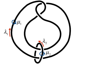
Figure 4: Whitehead link ($\mathbf{5}^{2}_{1}$). It is one of the simplest (having smallest volume $\simeq 3.664$) two-component hyperbolic link.

Whitehead link is denoted by $\mathbf{5}^{2}_{1}$, the 1st link with 2 components and 5 crossings, as shown in Fig. 4. The orientation of the link complement ($S^{3}\backslash\mathbf{5}^{2}_{1}$) is chosen as the one induced from an ideal triangulation in (259). We always choose a particular orientation of each ideal tetrahedron in an ideal triangulation which is reflected in the choice of CS level sign of $T_{\Delta}$ in (61). Then, the Dehn filled manifolds have natural orientation induced from the link complement. The overline in the equation $N=\overline{(S^{3}\backslash\mathbf{5^{2}_{1}})_{3\mu_{1}-2\lambda_{1}}}$ means that $N=m007$ has opposite orientation to the one induced from $S^{3}\backslash\mathbf{5}^{2}_{1}$ when the orientation of $N$ is chosen to be the one induced from an ideal triangulation in (157). The Dehn filling also gives an induced basis of $H_{1}(\partial N,\mathbb{Z})=\langle\mu_{2},\lambda_{2}\rangle$ on $N$ from the basis choice of $H_{1}(\partial(S^{3}\backslash\mathbf{5^{2}_{1}}),\mathbb{Z})=\langle\mu_{1},\mu_{2},\lambda_{1},\lambda_{2}\rangle$. From the topological fact that

$$N_{A}=(S^{3}\backslash\mathbf{5^{2}_{1}})_{3\mu_{1}-2\lambda_{1},\mu_{2}}=(S^{3}\backslash({\rm unknot}))_{3\mu-2\lambda}=L(3,-2)\;,$$ (156)

we see that $A$ is non-closable according to (152). The $N$ is a knot complement in a $\mathbb{Z}_{2}$-homological sphere, $N_{A}=L(3,-2)$, and according to (155) $A$ is of $SO(3)$ type. So from Table 1, we expect the $u(1)_{X_{\mu_{2}}}$ in $T^{DGG}[m007,X_{\mu_{2}}]$ is enhanced to $SO(3)$. Now, let us check the enhancement from explicit construction of the DGG theory. According to SnapPy, the knot complement can be triangulated by 3 ideal tetrahedra and the corresponding gluing data are (we choose $B=4\mu_{2}-\lambda_{2}$)

$$\begin{split}&C_{1}=Z_{1}+2Z_{2}+Z_{3}\;,\quad C_{2}=Z_{1}+Z_{1}^{\prime\prime}+Z_{2}^{\prime}+Z_{3}+Z_{3}^{\prime\prime}\;,\\ &C_{3}=2Z_{1}^{\prime}+Z_{1}^{\prime\prime}+Z_{2}^{\prime}+2Z_{2}^{\prime\prime}+2Z_{3}^{\prime}+Z_{3}^{\prime\prime}\;,\\ &a_{\mu_{2}}=-Z_{1}-Z_{1}^{\prime\prime}-Z_{2}+Z_{3}^{\prime\prime}+i\pi\;,\\ &b_{4\mu_{2}-\lambda_{2}}=2(-i\pi+Z_{1}+Z_{2})\end{split}$$ (157)

Since $(A,B)$ are of $(SO(3),SU(2))$-type, we choose

$$X_{\mu_{2}}=a_{\mu_{2}}\;,\quad P_{4\mu_{2}-\lambda_{2}}=\frac{1}{2}b_{4\mu_{2}-\lambda_{2}}\;.$$ (158)

Then, the symplectic matrix in (59) for this example is

$$\begin{split}&g_{m007}=\left(\begin{array}[]{cccccc}-1&-1&0&-1&0&1\\ 1&2&1&0&0&0\\ 1&-1&1&1&-1&1\\ 1&1&0&0&0&0\\ 0&0&0&0&0&1\\ 0&1&0&0&0&0\\ \end{array}\right)\;.\end{split}$$ (159)

The matrix can be decomposed into $g_{m007}=g^{s}_{J_{m007}}g^{t}_{K_{m007}}g^{gl}_{U_{m007}}$ with (68)

$$U_{m007}=\left(\begin{array}[]{ccc}1&1&0\\ 0&2&1\\ 0&1&0\end{array}\right)\;,\quad K_{m007}=\left(\begin{array}[]{ccc}1&0&0\\ 0&0&0\\ 0&-1&3\end{array}\right)\;,\quad J_{m007}=\left(\begin{array}[]{ccc}1&0&0\\ 0&0&0\\ 0&0&1\end{array}\right)\;.$$ (169)

Following each steps in eq. (61),(70) and (72), the Lagrangian for $T^{DGG}[m007,X_{\mu_{2}};P_{4\mu_{2}-\lambda_{2}}]$ is given by

$$\begin{split}&\mathcal{L}_{T^{DGG}[m007,X_{\mu_{2}};P_{4\mu_{2}-\lambda_{2}}]}\\ &=\int d^{4}\theta\left(\frac{1}{4\pi}\big{(}\frac{3}{2}\Sigma_{2}V_{2}+2V_{X}\Sigma_{1}+2V_{C}\Sigma_{2}\big{)}+\big{(}\Phi_{1}^{\dagger}e^{V_{1}-V_{2}}\Phi_{1}+\Phi_{2}^{\dagger}e^{V_{2}}\Phi_{2}+\Phi_{3}^{\dagger}e^{-V_{1}-V_{2}}\Phi_{3}\big{)}\right)\\ &\quad+\frac{1}{2}\int d^{2}\theta\Phi_{1}\Phi_{2}^{2}\Phi_{3}+(c.c)\;.\end{split}$$ (170)

In the Lagrangian, $V_{1}$ and $V_{2}$ are dynamical $u(1)$ vector multiplets. The superpotential term comes from an easy internal edge $C_{1}$, $O_{C_{1}}=\Phi_{1}\Phi_{2}^{2}\Phi_{3}$. The theory has $u(1)_{X_{\mu}}$ and $u(1)_{C}$ whose background vector multiplets are $V_{X}$ and $V_{C}$ respectively. Applying the mirror symmetry in eq. (77) and (80) with the following replacement

$$\Phi_{A}\rightarrow\Phi_{1},\Phi_{B}\rightarrow\Phi_{3},W\rightarrow V_{X}+V_{2},U\rightarrow-2V_{2}\;.$$ (171)

we have

$$\begin{split}&\mathcal{L}_{T^{DGG}[m007,X_{\mu_{2}};P_{4\mu_{2}-\lambda_{2}}]}\\ &=\frac{1}{4\pi}\int d^{4}\theta\big{(}\frac{3}{2}\Sigma_{2}V_{2}+2V_{C}\Sigma_{2}+\Phi_{2}^{\dagger}e^{V_{2}}\Phi_{2}+(T_{p})^{\dagger}e^{V_{X}+V_{2}}T_{p}+(T_{m})^{\dagger}e^{-V_{X}+V_{2}}T_{p}+M^{\dagger}e^{-2V_{2}}M\big{)}\\ &\quad+\bigg{(}\int d^{2}\theta M(\frac{1}{2}\Phi_{2}^{2}+T_{m}T_{p})+(c.c)\bigg{)}\;.\end{split}$$ (172)

In the dual picture, the $SO(3)$ symmetry is manifest after the redefinition of chiral fields as

$$\begin{split}&\phi_{1}:=\Phi_{2},\phi_{2}:=\frac{1}{\sqrt{2}}(T_{m}+T_{p}),\phi_{3}:=\frac{i}{\sqrt{2}}(T_{m}-T_{p})\;,\\ &\Rightarrow M(\frac{1}{2}\Phi_{2}^{2}+T_{m}T_{p})=\frac{1}{2}M(\phi_{1}^{2}+\phi_{2}^{2}+\phi_{3}^{2})\;.\end{split}$$ (173)

The $u(1)_{X}$ is in the Cartan of this $SO(3)$.

3.2 $SU(3)$ enhancement

From the point of view of 6d ${\cal N}=(2,0)$ theories, we only expect that the symmetry associated to codimension-2 defects (which are knots in 3-manifolds) are $su(2)$. However, we will see that there are many theories which have larger symmetry enhancement.

We consider a pair of $(N,A;B)$ and $(N^{\prime},A^{\prime};B^{\prime})$ such that

$$\begin{split}&1)\;\textrm{$A$ is of $SO(3)$ type while $A^{\prime}$ is of $SU(2)$ type}\;,\\ &2)\;\mathcal{I}_{N}^{(A,B)}(m,e;x)=\mathcal{I}_{N^{\prime}}^{(A^{\prime},B^{\prime})}(m,e;x)\;,\\ &3)\;\textrm{Both of $A$ and $A^{\prime}$ are non-closable cycles\;.}\end{split}$$ (174)

which we call $SU(3)$-enhancement pair. The $\mathcal{I}_{N}^{(A,B)}$ in 2) denotes a topological invariant called 3d index, see Appendix A. For such a pair, we claim that

$$\begin{split}&\textrm{I. Two theories $T^{DGG}[N,X_{A}]$ and $T^{DGG}[N^{\prime},X_{A^{\prime}}]$ are identical}\\ &\quad\;\textrm{possibly modulo a topological sector}\\ &\textrm{II. The theory has enhanced $SU(3)$ flavor symmetry where $SO(3)_{A}$ and $SU(2)_{A^{\prime}}$ are}\\ &\quad\;\textrm{embedded into the $SU(3)$ in a way that $\mathbf{3}_{SU(3)}\rightarrow\mathbf{3}_{SO(3)_{A}}$ and $\mathbf{3}_{SU(3)}\rightarrow(\mathbf{2}\oplus\mathbf{1})_{SU(2)_{A^{\prime}}}$}\;.\end{split}$$ (175)

The 3d index ${\cal I}_{N}^{(A,B)}(x)$ is equivalent to the superconformal index of $T^{DGG}[N,X_{A}]$ in charge basis. For hyperbolic complement $N$, the index is a non-trivial power series in $x$. The non-trivial match of the superconformal indices in the 2nd condition strongly suggests that two theories are actually equivalent possibly up to a topological sector.

From 1st and 3rd conditions in (174), the theory $T^{DGG}[N,X_{A}]=T^{DGG}[N^{\prime},X_{A^{\prime}}]$ has both of $SU(2)_{A}$ and $SO(3)_{A^{\prime}}$ symmetry where the $U(1)_{X_{A}}=U(1)_{X_{A}^{\prime}}$ is embedded into them as $\mathbf{2}_{SU(2)}=(\pm 1)_{U(1)}$ and $\mathbf{3}_{SO(3)}=(\pm 1,0)_{U(1)}$ respectively. The only consistency way of this happening is that the theory has a $SU(3)$ symmetry into which the $SU(2)_{A}$ and $SO(3)_{A^{\prime}}$ are embedded as II in (175). The reason is that the $SU(2)_{A}$ enhancement requires that there are conserved currents with charge $\pm 2$ under $U(1)_{X_{A}}$ from off-diagonal components of $SU(2)_{A}$, while the $SO(3)_{A^{\prime}}$ enhancement requires that there are conserved currents with charge $\pm 1$ under $U(1)_{X_{A}^{\prime}}$. Then the conserved currents with charge $\pm 1$ from $SO(3)_{A^{\prime}}$ is a doublet of $SU(2)_{A}$. A minimal completion of such a situation to a Lie algebra is to embed the symmetries to the $SU(3)$ algebra.

One may wonder if there exits such a pair. Surprisingly, we can find infinitely many examples of these pairs. A class of examples is

$$\begin{split}&N=(S^{3}\backslash\mathbf{5}^{2}_{1})_{\mu_{1}+k\lambda_{1}}\;,\quad A=\mu_{2}\;,\quad B=2\mu_{2}+\lambda_{2}\\ &N^{\prime}=\overline{(S^{3}\backslash\mathbf{5}^{2}_{1})_{(4k+1)\mu_{1}-k\lambda_{1}}}\;,\quad A^{\prime}=2\mu_{2}-\lambda_{2}\;,\quad B^{\prime}=\mu_{2}-\lambda_{2}\;.\end{split}$$ (176)

Figure 5: A rational surgery calculus rolfsen1984rational shows that $(S^{3}\backslash\mathbf{5^{2}_{1}})_{\mu_{2}+k\lambda_{2}}$ is a twist knot $K_{k}$. For example, $K_{k=1}=\mathbf{4_{1}},K_{k=-2}=\mathbf{5_{2}}$ and $K_{k=2}=\mathbf{6}_{1}$.

As shown in fig. 5, the $N$ above are nothing but twist knots which will be denoted as $K_{k}$. Let us check that the pair satisfy the 3 conditions in (174). First, note that both of $N$ and $N^{\prime}$ can be considered as a knot complement in $\mathbb{Z}_{2}$-homological spheres, $L(1,k)=(N)_{\mu_{2}}$ and $L(4k-1,-k)=(N^{\prime})_{\mu_{2}}$ respectively. Applying (155) with $\mu=\mu_{2}$ and $\lambda=\lambda_{2}$, we can conclude that $A/A^{\prime}$ is of $SO(3)/SU(2)$ type. Now let us check the 2nd condition in (174). Combining the $\mathbb{D}_{8}$-symmetry (261) of the Whitehead link index $\mathcal{I}_{\mathbf{5}^{2}_{1}}$ (260) and the following polarization transformation rules of 3d index

$$\begin{split}&\mathcal{I}_{S^{3}\backslash\mathbf{5}^{2}_{1}}^{(-\lambda_{1},\mu_{2};\mu_{1},2\mu_{2}+\lambda_{2})}(m_{1},m_{2},e_{1},e_{2};x)=\mathcal{I}_{\mathbf{5^{2}_{1}}}(e_{1},m_{2},-m_{1},e_{2}-m_{2};x)\\ &\mathcal{I}_{S^{3}\backslash\mathbf{5}^{2}_{1}}^{(4\mu_{1}-\lambda_{1},2\mu_{2}-\lambda_{2};\mu_{1},\lambda_{2}-\mu_{2})}(m_{1},m_{2},e_{1},e_{2})=\mathcal{I}_{\mathbf{5^{2}_{1}}}(e_{1},2m_{2}+e_{2},2e_{1}-m_{1},m_{2}+e_{2};x)\\ \end{split}$$ (177)

and the following matrix multiplication ($S_{2}$ is a generator of the $\mathbb{D}_{8}$ in (261))

$$\begin{split}&\left(\begin{array}[]{c}e_{1}\\ 2m_{2}+e_{2}\\ 2e_{1}-m_{1}\\ m_{2}+e_{2}\end{array}\right)_{(e_{1},e_{2})\rightarrow(-e_{1},-e_{2})}=S_{2}\cdot\left(\begin{array}[]{c}e_{1}\\ m_{2}\\ -m_{1}\\ e_{2}-m_{2}\end{array}\right)\;\end{split}$$ (178)

we have following identity

$$\mathcal{I}_{S^{3}\backslash\mathbf{5}^{2}_{1}}^{(-\lambda_{1},\mu_{2};\mu_{1},2\mu_{2}+\lambda_{2})}(m_{1},m_{2},e_{1},e_{2};x)=\mathcal{I}_{S^{3}\backslash\mathbf{5}^{2}_{1}}^{(4\mu_{1}-\lambda_{1},2\mu_{2}-\lambda_{2};\mu_{1},\lambda_{2}-\mu_{2})}(m_{1},m_{2},-e_{1},-e_{2};x)\;.$$ (179)

Applying the Dehn filling formula in eq. (255) to the above equality,

$$\begin{split}&\mathcal{I}_{(S^{3}\backslash\mathbf{5}^{2}_{1})_{\mu_{1}+k\lambda_{1}}}^{(\mu_{2};2\mu_{2}+\lambda_{2})}(m_{2},e_{2};x)=\mathcal{I}_{(S^{3}\backslash\mathbf{5}^{2}_{1})_{(4k+1)\mu_{1}-k\lambda_{1}}}^{(2\mu_{2}-\lambda_{2};\lambda_{2}-\mu_{2})}(m_{2},-e_{2};x)\;,\\ &\Rightarrow\mathcal{I}_{(S^{3}\backslash\mathbf{5}^{2}_{1})_{\mu_{1}+k\lambda_{1}}}^{(\mu_{2};2\mu_{2}+\lambda_{2})}(m_{2},e_{2};x)=\mathcal{I}_{\overline{(S^{3}\backslash\mathbf{5}^{2}_{1})_{(4k+1)\mu_{1}-k\lambda_{1}}}}^{(2\mu_{2}-\lambda_{2};\mu_{2}-\lambda_{2})}(m_{2},e_{2};x)\;,\quad\textrm{for all $k\in\mathbb{Z}$}\;.\end{split}$$ (180)

we confirm 2) in (174). In the above, we use the transformation rule of 3d index under the orientation reversal in (240). Finally, from the following topological facts martelli2002dehn

$$\begin{split}&N_{A}=(S^{3}\backslash\mathbf{5}^{2}_{1})_{\mu_{1}+k\lambda_{1},\mu_{2}}=L(1,k)\;,\\ &(N^{\prime})_{A^{\prime}}=(S^{3}\backslash\mathbf{5}^{2}_{1})_{(4k+1)\mu_{1}-k\lambda_{1},2\mu_{2}-\lambda_{2}}=L(-8k-2,-2k-1)\;,\end{split}$$ (181)

we see that both of $A$ and $A^{\prime}$ are non-closable cycles according to (152). So we confirm that the pair, $(N,A)$ and $(N^{\prime},A^{\prime})$, in (176) satisfy all the conditions in (174) and the corresponding DGG theory is expected to have $SU(3)$ flavor symmetry. We will check the ehancement explicitly for $k=1,-2$ by explicitly constructing $T^{DGG}[N,A]$ and $T^{DGG}[N^{\prime},A^{\prime}]$.

For $k=1$

In the case,

$$\begin{split}&(S^{3}\backslash\mathbf{5}^{2}_{1})_{\mu_{1}+\lambda_{1}}=(S^{3}\backslash\mathbf{4}_{1})=m004\;,\\ &\overline{(S^{3}\backslash\mathbf{5}^{2}_{1})_{5\mu_{1}-\lambda_{1}}}=(\textrm{Sister of }S^{3}\backslash\mathbf{4}_{1})=m003\;.\end{split}$$ (182)

$m003$ is a knot complement called sister of figure-eight knot complement. Both 3-manifolds have the same hyperbolic volume and are the smallest hyperbolic 3-manifolds with one cusp torus boundary. From ideal triangulations of $m003$ and $m004$ given below, their orientation are fixed. The equality in the above means not only that the two manifolds are homeomorphism but also that they have the same orientation, i.e. the orientation of $m004$ is same as the orientation induced from a Dehn filling on $S^{3}\backslash\mathbf{5^{2}_{1}}$, whose orientation is induced from an ideal triangulation in (259).

According to SnapPy, both can be ideally triangulated by two tetrahedra and have common internal edge variables given in (87) while boundary variables are different by a factor $2$ or $1/2$

$$\begin{split}&a_{\mu_{2}}=Z_{1}-Z_{2}\;,\quad b_{\lambda_{2}+2\mu_{2}}=4Z_{1}-2Z_{1}^{\prime}-2Z_{2}\;,\quad\textrm{ for $m004$}\;.\\ &a_{2\mu_{2}-\lambda_{2}}=2Z_{1}-2Z_{2}\;,\quad b_{\mu_{2}-\lambda_{2}}=2Z_{1}-Z_{1}^{\prime}-Z_{2}\;,\quad\textrm{ for $m003$}\;.\end{split}$$ (183)

For DGG’s construction, we choose

$$\begin{split}&X_{\mu_{2}}=a_{\mu_{2}}\;,\quad P_{2\mu_{2}+\lambda_{2}}=\frac{1}{2}b_{2\mu_{2}+\lambda_{2}}\;,\quad\textrm{ for $m004$}\;.\\ &X_{2\mu_{2}-\lambda_{2}}=\frac{1}{2}a_{2\mu_{2}-\lambda_{2}}\;,\quad P_{\mu_{2}}=b_{\mu_{2}-\lambda_{2}}\;,\quad\textrm{ for $m003$}\;.\end{split}$$ (184)

Thus, both DGG theories are identical and described by the Lagrangian in (104) up to background CS level for $U(1)_{X}$ which is irrelevant in symmetry enhancement. We reproduce the Lagrangian here with the modified background CS level;

$$\begin{split}&\mathcal{L}_{T^{DGG}[m004,X_{\mu_{2}};P_{2\mu_{2}+\lambda_{2}}]}(V_{X},V_{C})=\mathcal{L}_{T^{DGG}[m003,X_{2\mu_{2}-\lambda_{2}};P_{\mu_{2}-\lambda_{2}}]}(V_{X},V_{C})\\ &=\frac{1}{4\pi}\int d^{4}\theta\left(-\frac{1}{2}\Sigma_{C}V_{X}+\Sigma(2V_{C}+3V_{X})+\Sigma_{X}V_{X}\right)+\int d^{4}\theta\left(\Phi_{1}^{\dagger}e^{V+\frac{V_{X}}{2}}\Phi_{1}+\Phi_{2}^{\dagger}e^{V-\frac{V_{X}}{2}}\Phi_{2}\right)\;.\end{split}$$ (185)

So the theory is

$$\begin{split}&T^{DGG}[m004,\mu_{2}]=T^{DGG}[m003,2\mu_{2}-\lambda_{2}]\\ &=\textrm{A $U(1)$ vector multiplet coupled to 2 chirals of charge $+1$}\;.\end{split}$$ (186)

The theory has manifest $u(1)_{\rm top}\times su(2)_{\rm manifest}$ where $u(1)_{\rm top}$ is the topological monopole charge of the $u(1)_{\rm gauge}$ gauge symmetry, and $su(2)_{\rm manifest}$ acts on the two chiral fields. This $u(1)_{\rm top}\times su(2)_{\rm manifest}$ will be enhanced to $SU(3)$.

The $u(1)_{C}$ flavor symmetry associated to the background field $V_{C}$ corresponds to the topological symmetry $u(1)_{\rm top}$ and will be embedded to $SU(3)$ as

$$u(1)_{C}=u(1)_{\rm top}=T_{8}:=\textrm{diag}(-1/3,-1/3,2/3)\in SU(3)\;.$$ (187)

This is because the “off-diagonal components” of $SU(3)$ (which are not in $u(1)_{C}\times su(2)_{\rm manifest}$) are provided by monopole operators with monopole charge $\pm 1=\pm(1/3-(-2/3))$.

On the other hand, the $V_{X}$ is coupled to the system as follows. Let

$$T_{3}:=\textrm{diag}(1/2,-1/2,0)\;.$$ (188)

be the Cartan generator of the manifest $su(2)_{\rm manifest}$. The $V_{X}$ is coupled to the chiral fields via this generator $T_{3}$. Also, notice that $V_{X}$ is coupled to the monopole current $\Sigma$ with coefficients $3/2$. Therefore the $u(1)_{X}$ is embedded in $SU(3)$ as

$$u(1)_{X}=\frac{3}{2}T_{8}+T_{3}=\textrm{diag}(0,-1,1)\in SU(3)\;.$$ (189)

This $u(1)_{X}$ must be enhanced to $su(2)_{X}$ because the $A$-cycle is non-closable.

Notice that this $su(2)_{X}$ is different from the manifest $su(2)_{\rm manifest}$ symmetry. Therefore, if $u(1)_{X}$ is enhanced to $su(2)_{X}$, then the $u(1)_{\rm top}\times su(2)_{\rm manifest}$ must be enhanced to $SU(3)$. This agrees with our general discussion that this theory has enhanced $SU(3)$ symmetry.

The superconformal index of theory is

$$\begin{split}&\mathcal{I}_{m003/m004}(u_{1},u_{2};x)\\ &=\sum_{(e_{1},e_{2})\in\mathbb{Z}^{2}}(-x^{\frac{1}{2}})^{e_{2}}\mathcal{I}_{\Delta}(-e_{2},-e_{1}+2e_{2};x)\mathcal{I}_{\Delta}(-e_{2},e_{1}-e_{2};x)u_{1}^{e_{1}}u_{2}^{e_{2}}\;.\end{split}$$ (190)

Here $u_{1}$ and $u_{2}$ fugacity variable for $u(1)_{X}$ and $u(1)_{C}$ symmetry respectively. The index depends on the choice of $R$-charge mixing between $u(1)_{R}$ and $u(1)_{C}$. In the above expression, we in particularly choose,

$$R(\Phi_{a})=\frac{1}{3},\quad R(V_{\pm})=\frac{2}{3}\;.$$ (191)

Here $V_{\pm}$ denote a BPS monopole operator of charge $\pm 1$. Then the index show the $SU(3)$ structure :

$$\begin{split}&\mathcal{I}_{m003/m004}(u_{1},u_{2};x)=1-(\chi_{1,1})x-(\chi_{0,0}+\chi_{1,1})x^{2}+(\chi_{2,2}-\chi_{0,0}-\chi_{1,1})x^{3}\\ &\qquad\quad+(\chi_{3,0}+\chi_{2,2}+\chi_{0,3}-\chi_{0,0})x^{4}+(\chi_{0,3}+2\chi_{1,1}+2\chi_{2,2}+\chi_{3,0})x^{5}+\ldots\end{split}$$ (192)

Here $\chi_{m,n}(u_{1},u_{2})$ is the character of $SU(3)$-representation with Dynkin labels $(m,n)$. The correct IR R-charge mixing should be determined by F-maximization, but the non-trivial appearance of the $SU(3)$ in a particular choice strongly suggests that the choice gives the correct R-charge assignment. The first non-trivial terms comes form operators listed in the Table below.

	$u(1)_{C}$	$u(1)_{X}$	SCI contribution
$\phi_{a}(\psi^{*}_{+})_{b}$	0	$\pm\frac{1}{2}\pm\frac{1}{2}$	$-(2+u_{1}+\frac{1}{u_{1}})x$
$V_{-}(\phi_{a})$	$1$	$(1,2)$	$-(u_{1}u_{2}+u_{1}^{2}u_{2})x$
$V_{+}(\phi_{a})$	$-1$	$(-1,-2)$	$-(\frac{1}{u_{1}^{2}u_{2}}+\frac{1}{u_{1}u_{2}})x$

In the table, $\phi_{a}$ and $(\psi_{\pm})_{a}$ denote the scalar and fermionic fields in chiral field $\Phi_{a}$ respectively with $a=1,2$. $V_{\pm}(\ldots)$ denote a gauge invariant BPS monopole operator of charge $\pm 1$ dressed by matter fields $(\ldots)$. All these operators have quantum numbers $(R,j_{3},\Delta)=(1,\frac{1}{2},\frac{3}{2})$ and form descents of conserved current multiplet for $SU(3)$ flavor symmetry. In 3d $\mathcal{N}=2$ SCFT, a conserved current multiplet of flavor group $F$ consists of following operators in the adjoint representation of $F$:

$$[0]^{(0)}_{\Delta=1}\xrightarrow[\text{}]{\;Q,\tilde{Q}\;}[\frac{1}{2}]^{(1)}_{\Delta=\frac{3}{2}}\oplus[\frac{1}{2}]^{(-1)}_{\Delta=\frac{3}{2}}\xrightarrow[\text{}]{\;Q,\tilde{Q}\;}[1]^{(0)}_{\Delta=2}\oplus[0]^{(0)}_{\Delta=2}$$ (193)

Here operators are denoted by its quantum number $[j]^{(r)}_{\Delta}$ where $j$ denote a spin of space-time rotational symmetry $su(2)$ in a normalization such that $[1/2]$ corresponds to the fundamental representation.

For $k=-2$

In the case,

$$\begin{split}&(S^{3}\backslash\mathbf{5}^{2}_{1})_{\mu_{1}-2\lambda_{1}}=\overline{S^{3}\backslash\mathbf{5}_{2}}=\overline{m015};,\\ &\overline{(S^{3}\backslash\mathbf{5}^{2}_{1})_{-7\mu_{1}+2\lambda_{1}}}=\overline{m017}\;.\end{split}$$ (194)

Both manifolds have the same hyperbolic volume $\textrm{vol}(m015)=\textrm{vol}(m017)=2.82812\ldots$. According to SnapPy, both can be ideally triangulated by three tetrahedra and have common internal edge variables

$$\begin{split}&C_{1}=Z_{1}^{\prime}+Z_{1}^{\prime\prime}+2Z_{2}+Z_{3}^{\prime}+Z_{3}^{\prime\prime}\;,\quad C_{2}=Z_{1}+Z_{1}^{\prime}+Z_{2}^{\prime}+Z_{3}+Z_{3}^{\prime}\;,\\ &C_{3}=Z_{1}+Z_{1}^{\prime\prime}+Z_{2}^{\prime}+2Z^{\prime\prime}_{2}+Z_{3}+Z_{3}^{\prime\prime}\;.\end{split}$$ (195)

while boundary variables are different by a factor $2$ or $1/2$

$$\begin{split}&a_{\mu_{2}}=-Z_{1}+Z_{2}\;,\quad b_{-2\mu_{2}-\lambda_{2}}=2(2Z_{1}-Z_{1}^{\prime\prime}-2Z_{2}+Z_{3}^{\prime\prime})\;,\quad\textrm{ for $m015$}\;.\\ &a_{2\mu_{2}-\lambda_{2}}=-2Z_{1}+2Z_{2}\;,\quad b_{\lambda_{2}-\mu_{2}}=2Z_{1}-Z_{1}^{\prime\prime}-2Z_{2}+Z_{3}^{\prime\prime}\;,\quad\textrm{ for $m017$}\;.\end{split}$$ (196)

We choose

$$\begin{split}&X_{\mu_{2}}=a_{\mu_{2}}\;,\quad P_{-2\mu_{2}-\lambda_{2}}=\frac{1}{2}b_{-2\mu_{2}-\lambda_{2}}\;,\quad\textrm{ for $m015$}\;.\\ &X_{2\mu_{2}-\lambda_{2}}=\frac{1}{2}a_{2\mu_{2}-\lambda_{2}}\;,\quad P_{\mu_{2}}=b_{\lambda_{2}-\mu_{2}}\;,\quad\textrm{ for $m017$}\;.\end{split}$$ (197)

Then, the $Sp(6,\mathbb{Z})$+(affine-shifts) are

$$\begin{split}&\left(\begin{array}[]{c}X\\ C_{1}\\ C_{2}\\ P\\ \Gamma_{1}\\ \Gamma_{2}\end{array}\right)=g_{m0015/m017}\cdot\left(\begin{array}[]{c}Z_{1}\\ Z_{2}\\ Z_{3}\\ Z_{1}^{\prime\prime}\\ Z_{2}^{\prime\prime}\\ Z_{3}^{\prime\prime}\end{array}\right)+i\pi\nu_{m015/m017}\\ &g_{m015/m017}=\left(\begin{array}[]{cccccc}-1&1&0&0&0&0\\ -1&2&-1&0&0&0\\ 0&-1&0&-1&-1&-1\\ 2&-2&0&-1&0&1\\ 0&0&0&0&0&-1\\ 0&1&0&0&0&0\\ \end{array}\right)\;,\quad\nu_{m015/m017}=\left(\begin{array}[]{c}0\\ -2\\ -3\\ 0\\ 0\\ 0\end{array}\right)\end{split}$$ (198)

The matrix $g_{m015/m017}$ can be decomposed into $g_{m015/m017}=g^{s}_{J_{m015}}g^{t}_{K_{m015}}g^{gl}_{U_{m015}}$ (68)

$$U_{m015}=\left(\begin{array}[]{ccc}-1&1&0\\ -1&2&-1\\ 0&1&0\\ \end{array}\right)\;,\quad K_{m015}=\left(\begin{array}[]{ccc}-2&0&0\\ 0&0&0\\ 0&0&1\\ \end{array}\right)\;,\quad J_{m015}=\left(\begin{array}[]{ccc}0&0&0\\ 0&0&0\\ 0&0&1\\ \end{array}\right)\;.$$ (208)

Using the decomposition, we have

$$\begin{split}&\mathcal{L}_{T^{DGG}[m015,X_{\mu_{2}};P_{-2\mu_{2}-\lambda_{2}}]}(V_{X},V_{C_{1}},V_{C_{2}})=\mathcal{L}_{T^{DGG}[m017,X_{2\mu_{2}-\lambda_{2}};P_{\lambda_{2}-\mu_{2}}]}(V_{X},V_{C_{1}},V_{C_{2}})\\ &=\frac{1}{4\pi}\int d^{4}\theta\big{(}-3\Sigma_{X}V_{X}+\Sigma_{X}V_{C_{1}}-\frac{1}{2}(\Sigma_{C_{1}}-\Sigma)(V_{C_{1}}-V)+2\Sigma V_{C_{2}}\big{)}\\ &\quad+\int d^{4}\theta\big{(}\Phi_{1}^{\dagger}e^{V-V_{X}}\Phi_{1}+\Phi_{2}^{\dagger}e^{V}\Phi_{2}+\Phi_{3}^{\dagger}e^{V+V_{X}-V_{C_{1}}}\Phi_{3}\big{)}\;.\end{split}$$ (209)

Here $V$ is a dynamical $u(1)$ vector multiplet. Since $C_{1}$ and $C_{2}$ are hard internal edges and we can not add $O_{C_{1}}$ and $O_{C_{2}}$ to superpotential. So, the DGG theory is

$$\begin{split}&T^{DGG}[m015,\mu_{2}]=T^{DGG}[m017,2\mu_{2}-\lambda_{2}]\\ &=\textrm{A $u(1)_{-1/2}$ vector multiplet coupled to 3 chirals of charge $+1$}\;.\end{split}$$ (210)

The theory has manifest $SU(3)$ flavor symmetry rotating 3 chrials as expected.

4 Dehn filling in 3d/3d correspondence

In this section, we generalize the DGG’s construction to obtain $T^{6d}_{\rm irred}[M]$ for closed 3-manifolds $M$ by incorporating Dehn filling operation. Refer to Pei:2015jsa ; Gadde:2013sca ; Gukov:2017kmk ; Alday:2017yxk for previous discussions on Dehn filling operation in the context of 3d/3d correspondence and the construction of 3d theory, which we will denote $T^{6d}_{(\rm irred)^{c}}[M]$, labelled by Seifert manifolds $M$.

4.1 Dehn filling on $T^{6d}_{\rm irred}[N]$

For a hyperbolic knot complement $N$ and a primitive boundary cycle $(pA+qB)\in H_{1}(\partial N,\mathbb{Z})$,

$$T^{6d}_{\rm irred}[N_{pA+qB}]=(\textrm{Giving a nilpotent vev to $\mu$ of $T^{6d}_{\rm irred}[N,pA+qB]$})\;.$$ (211)

The fact that the closing of codimension-2 defects (i.e., knots) corresponds to giving the nilpotent vev to $\mu$ is standard in 4d class S theories. See e.g., Tachikawa:2013kta and references therein. This is also in accord with our terminology ‘closable/non-closable’, because non-closable cycles have empty $\mu$ and hence it is not possible to do the above operation while preserving supersymmetry. See Table 3 below.

$pA+qB\in H_{1}\big{(}\partial N,\mathbb{Z}\big{)}$	$T^{6d}_{\rm irred}[N_{pA+qB}]$
non-exceptional ($\Rightarrow$ closable)	non-trivial SCFT
exceptional and closable	Gapped theory (possibly with decoupled free chirals)
non-closable	SUSY broken

Table 3: Basic property of $T^{6d}_{\rm irred}[N_{pA+qB}]$. A primitive boundary cycle $pA+qB$ is called exceptional if $N_{pA+qB}$ is non-hyperbolic.

If the $A$ is non-closable and $q=1$, the above relation can be simplified as follows. The theory $T^{6d}_{\rm irred}[N,pA+B]$ is related to the theory $T^{6d}_{\rm irred}[N,A;B]$ by the transformation $ST^{p}\in SL(2,{\mathbb{Z}})$ as

$$T^{6d}_{\rm irred}[N,pA+B]=T^{6d}_{\rm irred}[N,A;B]-su(2)_{p}-T[SU(2)],$$ (212)

where $su(2)_{p}$ is gauging the $su(2)$ symmetry of $T^{6d}_{\rm irred}[N,A;B]$ and the $su(2)_{H}$ symmetry of $T[SU(2)]$. The Chern-Simons level of this group is $p+[\text{original value}]$, where $[\text{original value}]$ means the contribution of $T^{6d}_{\rm irred}[N,A;B]$ to the Chern-Simons level. To specify this contribution, we have to specify not only the $A$-cycle, but also the $B$-cycle. This is the reason why we are writing $B$ explicitly in the notation $T^{6d}_{\rm irred}[N,A;B]$.

Now, the operator $\mu$ comes from the moment map operator of $T[SU(2)]$ associated to the $su(2)_{C}$ symmetry which is not gauged. If we give a nilpotent vev to this operator $\mu$, the $T[SU(2)]$ becomes massive and flows to an empty theory in the low energy limit up to the Goldstone multiplets associated to the symmetry breaking of $su(2)_{C}$ by the vev Gaiotto:2008ak . Neglecting those Goldstone multiplets, the $T[SU(2)]$ disappears and hence we get

$$\begin{split}T^{6d}_{\rm irred}[N_{pA+B}]&=(\textrm{Gauging $su(2)$ of $T^{6d}_{\rm irred}[N,A;B]$ with additional CS level $p$})\;,\\ &=(\textrm{Gauging $su(2)$ of $T^{DGG}[N,A;B]$ with additional CS level $p$})\;.\end{split}$$ (213)

where we have assumed that $A$ is non-closable and hence $T^{6d}_{\rm irred}[N,A;B]=T^{DGG}[N,A;B]$.

As examples, we consider closed 3-manifolds obtained from $m003/m004/m015$ by performing a Dehn filling. Combing (185),(209) and (213), we have

$$\begin{split}&T^{6d}_{\rm irred}[(m003)_{p(2\mu_{2}-\lambda_{2})+(\mu_{2}-\lambda_{2})}=\overline{(S^{3}\backslash\mathbf{5}^{2}_{1})_{5\mu_{1}-\lambda_{1},~{}p(2\mu_{2}-\lambda)+(\mu_{2}-\lambda_{2})}}]\\ &=\frac{\textrm{A $u(1)_{0}$ vector coupled to 2 chrials of charge +1}}{SU(2)_{p+1/2}}\;,\\ &T^{6d}_{\rm irred}[(m004)_{p\mu_{2}+(\lambda_{2}+2\mu_{2})}=(S^{3}\backslash\mathbf{4}_{1})_{(p+2)\mu+\lambda}]\\ &=\frac{\textrm{A $u(1)_{0}$ vector coupled to 2 chrials of charge +1}}{SO(3)_{p+2}}\;,\\ &T^{6d}_{\rm irred}[(m015)_{p\mu_{2}+(-2\mu_{2}-\lambda_{2})}=(S^{3}\backslash\mathbf{5}_{2})_{(p-2)\mu+\lambda}]\\ &=\frac{\textrm{A $u(1)_{-1/2}$ vector coupled to 3 chrials of charge +1}}{SO(3)_{p-6}}\;.\end{split}$$ (214)

Here the notation $/G_{k}$ means that we couple a vector multiplet of group $G$ with the Chern-Simons level $k$. The theories in the numerator has $SU(3)$ symmetry at IR as argued in sec. 3.2 and we are gauging its $SO(3)/SU(2)$ subgroup. Since the $u(1)_{X}$ is embedded to the $SU(2)$ (resp. $SO(3)$) in a way that $\mathbf{2}_{su(2)}=(\pm 1)_{u(1)_{X}}$ (resp. $\mathbf{2}_{su(2)}=(\pm\frac{1}{2})_{u(1)_{X}}$), the CS level $+1$ for $u(1)_{X}$ in (185) corresponds to CS level $1/2$ (resp. 2) for the $su(2)$. Similarly the CS level $-3$ for $u(1)_{X}$ in (209) corresponds to CS level $-6$ for the $su(2)$. A parity operation filps the signs of CS levels of the $T^{6d}_{\rm irred}$ theories. The parity operation corresponds to orientation reversal on the internal 3-manifold. It is compatible with following topological facts

$$\begin{split}&(m003)_{p(2\mu_{2}-\lambda_{2})+(\mu_{2}-\lambda_{2})}=\overline{(m003)_{(-p-1)(2\mu_{2}-\lambda_{2})+(\mu_{2}-\lambda_{2})}}\;,\\ &(m004)_{p\mu_{2}+(\lambda_{2}+2\mu_{2})}=\overline{(m004)_{(-p-4)\mu_{2}+(\lambda_{2}+2\mu_{2})}}\;.\end{split}$$ (215)

After gauging $SU(2)/SO(3)$ subgroup of $SU(3)$, the resulting theory generically has following flavor symmetry

$$\begin{split}&T^{6d}_{\rm irred}[(S^{3}\backslash\mathbf{5}^{2}_{1})_{5\mu_{1}-\lambda_{1},~{}p(2\mu_{2}-\lambda)+(\mu_{2}-\lambda_{2})}]\;\textrm{has $u(1)$ flavor symmetry }\\ &T^{6d}_{\rm irred}[(S^{3}\backslash\mathbf{4}_{1})_{(p+2)\mu_{2}+\lambda_{2}}]\;\textrm{has no flavor symmetry }\\ &T^{6d}_{\rm irred}[(S^{3}\backslash\mathbf{5}_{2})_{(p-2)\mu+\lambda}]\;\textrm{has $u(1)$ flavor symmetry }\end{split}$$ (216)

The $u(1)$ for the 3rd case comes from the topological symmetry of $u(1)_{-1/2}$ gauge symmetry of the theory in the numerator. The above is correct when $|p|$ is large enough where the semiclassical analysis is reliable. When $|p|$ is small, the theories could have accidental symmetries. Actually from following topological fact (see Figure. 6),

$$(S^{3}\backslash\mathbf{4}_{1})_{-5\mu+\lambda}=(S^{3}\backslash\mathbf{5}_{2})_{5\mu+\lambda}$$ (217)

we can conclude that $T^{6d}_{\rm irred}[(S^{3}\backslash\mathbf{4}_{1})_{(p+2)\mu_{2}+\lambda_{2}}]$ has accidental $u(1)$ symmetry for $p=3$ and $p=-7$. We will come back to this point in sec 5.

4.2 Small hyperbolic manifolds

Let us discuss the case of closed 3-manifolds $M=$Weeks, a oriented hyperbolic closed 3-manifold with smallest hyperbolic volume. This was already discussed in Gang:2017lsr and here we supply a little bit more details. The Weeks manifold is obtained by performing a Dehn filling operation on $m003$,

$$\overline{(S^{3}\backslash\mathbf{5}^{2}_{1})_{5\mu_{1}-\lambda_{1},-5\mu_{2}+2\lambda_{2}}}=(m003)_{-5\mu_{2}+2\lambda_{2}}=\textrm{Weeks}\;.$$ (218)

Corresponding 3d gauge theory is the theory in the second line of eq. (214) with $p=-3$. The theory in the numerator has $SU(2)_{X}$ symmetry which is a subgroup of the $SU(3)$. The $SU(2)_{X}$ symmetry is different from the manifest $SU(2)_{\rm manifest}$ rotating two chirals. But using the Weyl symmetry of the $SU(3)$, the symmetry $SU(2)_{X}$ and $SU(2)_{\rm manifest}$ can be exchanged with each other. Therefore, we can take $SU(2)_{X}$ to be the manifest $SU(2)_{\rm manifest}$. We will just denote it as $SU(2)$ in the following. Then by (214),

$$T^{6d}_{\rm irred}[\text{Weeks}]=\text{(Two chiral fields coupled to $U(1)_{0}\times SU(2)_{-5/2}$)}.$$ (219)

AF duality

Now, we can further simplify this theory to a much simpler theory Gang:2017lsr . There is a duality found by Aharony and Fleischer (AF) Aharony:2014uya

$$\text{(Two chiral fields coupled to $SU(2)_{-5/2}$)}=\text{(One chiral field gauged by $U(1)_{+3/2}$)}.$$ (220)

To apply this duality, we need to know the relation between the flavor $U(1)$ symmetries of both sides of this equation and their background Chern-Simons levels.

Here we supply the details promised in Gang:2017lsr . In the AF duality, the $U(1)$ charge acting on two chiral fields with charge 1 on the left hand side corresponds to the topological charge of the $U(1)_{+3/2}$ gauge field multiplied by 2. The reason is that the $-1\in U(1)$ acting on the two chiral fields can be compensated by the $-1\in SU(2)_{-5/2}$ gauge transformation, and hence all gauge invariant operators have even charge on the left hand side. So the relation is

$$SU(2)_{-5/2}-\text{two chirals }-U(1)^{\rm bkg}_{0}$$

$$\Longleftrightarrow~{} \text{single chiral}-U(1)_{3/2}\overset{\times 2}{-}U(1)^{\rm bkg}_{n}.$$ (221)

where $U(1)^{\rm bkg}$ is the global symmetry with background field, $n$ is the background Chern-Simons level, and $\times 2$ means that the $U(1)^{\rm bkg}_{n}$ is coupled to the topological current of $U(1)_{3/2}$ multiplied by two.

We want to determine the value of $n$. This can be done as follows. Let $\sigma^{\rm bkg}$ be the real scalar for the background $U(1)^{\rm bkg}$ vector multiplet, or in other words, the real mass associated to this symmetry. We choose the sign of it such that after integrating out the two chiral fields on the left hand side, the left hand side flows to

$$SU(2)_{-3}\oplus U(1)^{\rm bkg}_{-1}.$$ (222)

where $\oplus$ means that the two factors $SU(2)_{3}$ and $U(1)^{\rm bkg}_{1}$ are completely decoupled. Here we need to remark the important point. The $SU(2)_{-3}$ is the 3d ${\cal N}=2$ gauge theory at the level $-3$. This theory contains the gaugino, and by integrating out the gaugino, we get a pure topological Chern-Simons theory as

$$SU(2)_{-3}=SU(2)^{\text{topo CS}}_{-1}$$ (223)

Namely, the gaugino reduces the level by $2=h^{\vee}_{su(2)}$. Therefore, the low energy limit is

$$SU(2)^{\text{topo CS}}_{-1}\oplus U(1)^{\rm bkg}_{-1}$$ (224)

The effect of $\sigma^{\rm bkg}$ on the right-hand-side of (221) is to give the dynamical $U(1)$ an FI parameter. We want the dynamical gauge group $U(1)$ to be not Higgsed so that we can match it with the $SU(2)^{\text{topo CS}}_{-1}$ later. Then, the D-term condition implies that the dynamical real scalar $\sigma$ gets a vev proportional to $\sigma^{\rm bkg}$ because the Lagrangian contains $3/2D\sigma+2\cdot 2D\sigma^{\rm bkg}$ and we need to impose stationary condition for $D$. The vev of $\sigma$ gives the chiral field a mass term. The sign of the mass is anticipated by the fact that it must make the low energy CS level of the dynamical field as $U(1)_{-2}$. This is because the only consistent way for the duality to work in low energy is to use the duality of topological CS theory given by

$$SU(2)^{\text{topo CS}}_{-1}=U(1)^{\text{topo CS}}_{-2}\sim U(1)^{\text{topo CS}}_{2}$$ (225)

where we have used the fact that the gaugino plays no role in $U(1)$ and hence $U(1)_{-2}=U(1)^{\text{topo CS}}_{-2}$. First equality is well-known (see, e.g., DiFrancesco:1997nk for the corresponding statement in Wess-Zumino-Witten models which are related to topological Chern-Simons theories Witten:1988hf .). The second equality $U(1)^{\text{topo CS}}_{2}\sim U(1)^{\text{topo CS}}_{-2}$ is more precisely given by $U(1)_{2}\times U(1)_{-1}=U(1)_{-2}\times U(1)_{1}$ Seiberg:2016rsg ; Tachikawa:2016cha ; Tachikawa:2016nmo and we have neglected $U(1)_{\pm 1}$ because these theories have only one state in the Hilbert space on any space (and they are called invertible field theory), and our argument is not careful enough to detect those invertible field theories.

After integrating out the chiral field, the right-hand-side of (221) is given by the Lagrangian

$$\frac{1}{4\pi}\left(2V\Sigma+2\cdot 2V\Sigma^{\rm bkg}+nV^{\rm bkg}\Sigma^{\rm bkg}\right).$$ (226)

where in the second term, the factor of $2$ have taken into account the fact that $\mathrm{U}(1)^{\rm bkg}$ is coupled to the topological current of $\mathrm{U}(1)$ by charge $2$. We shift the dynamical gauge field as $V\to V+V^{\rm bkg}$ to get

$$\frac{1}{4\pi}\left(2V\Sigma+(n-2)V^{\rm bkg}\Sigma^{\rm bkg}\right).$$ (227)

This means that the low energy theory is given by

$$U(1)^{\text{topo CS}}_{2}\oplus U(1)^{\rm bkg}_{n-2}.$$ (228)

Therefore by comparing the low energy limit of the left and right hand side of (221), we get

$$-1=n-2\Longrightarrow n=1.$$ (229)

Weeks theory

Now let us gauge $U(1)^{\rm bkg}$ (but we use the same name for simplicity). The left hand side of (221) after gauging $U(1)^{\rm bkg}$ is precisely the theory $T^{6d}_{\rm irred}[\text{Weeks}]$.

Let us see the right hand side. The Chern-Simons action of the right-hand-side of (221) after putting $n=1$ is given by

$$\frac{1}{4\pi}\left(\frac{3}{2}V\Sigma+2\cdot 2V\Sigma^{\rm bkg}+V^{\rm bkg}\Sigma^{\rm bkg}\right).$$ (230)

where in the second term, the factor of $2$ have taken into account the fact that $U(1)^{\rm bkg}$ is coupled to the topological current of $U(1)_{3/2}$ by charge $2$. If we integrate out $V^{\rm bkg}$, or in other words, by making the shift $V^{\rm bkg}\to V^{\rm bkg}+2V$ and neglecting the decoupled $U(1)_{1}$ theory, we get

$$\frac{1}{4\pi}\left((\frac{3}{2}-4)V\Sigma\right)=\frac{1}{4\pi}\left(-\frac{5}{2}V\Sigma\right).$$ (231)

We conclude that the theory $T^{6d}_{\rm irred}[\text{Weeks}]$ is given by

$$T^{6d}_{\rm irred}[\text{Weeks}]=(\text{One chiral field coupled to $U(1)_{-5/2}$}).$$ (232)

This is one of the small theories discussed in Gang:2017lsr .

5 3d $\mathcal{N}=2$ Dualities from Surgery calculus

The DGG’s construction is based on an ideal triangulation of a knot complement $N$. Different ideal triangulations give different field theory descriptions of $T^{DGG}[N]$ theory related by a duality. In our construction $T^{6d}_{\rm irred}[M]$ for a closed 3-manifold $M$, we use a Dehn filling description of the closed 3-manifold, $M=N_{A}$, with a hyperbolic knot complement $N$ and a primitive boundary cycle $A$. The construction can be straightforwardly generalized to the case when $M$ can be given by Dehn fillings on a link complement. According to the Lickorish-Wallace theorem Lickorish Wallace , every closed orientable 3-manifold $M$ can be obtained by performing Dehn surgery along a link $L$ in $S^{3}$.

$$\begin{split}M&=(S^{3}\backslash L)_{p_{1}\mu_{1}+q_{1}\lambda_{1},p_{2}\mu_{2}+q_{2}\lambda_{2},\ldots,p_{l}\mu_{l}+q_{l}\lambda_{l}}\;,\quad\textrm{$l=|L|$ : $\sharp$ of components of a link $L$}\;.\end{split}$$ (233)

The Dehn surgery representation is not unique and there are different choices of $(L,\{p_{i},q_{i}\})$ and $(L^{\prime},\{p_{i}^{\prime},q_{i}^{\prime}\})$ which give a same closed 3-manifold. Different Dehn surgery presentations of $M$ give different gauge theory descriptions of $T^{6d}_{\rm irred}[M]$ related by a 3d duality. A rational surgery calculus rolfsen1984rational studies the equivalence relation among the choices. Every pair of equivalent Dehn surgery representations are known to be related by a sequence of basic local moves depicted in figure  6. The basic moves may corresponds to basic 3d $\mathcal{N}=2$ dualities among $T^{6d}_{\rm irred}[M]$. Identifying the basic dualities would be interesting and we leave it as future work.

Figure 6: Left : Basic moves in rational surgery calculus rolfsen1984rational . The rational number $r_{i}$ next to $i$-th component of link $K$ represent Dehn filling slope and $\mathbf{lk}(i,1)$ denotes the linking number between $i$-th component and 1st component. Right: A sequence of basic moves showing $(S^{3}\backslash\mathbf{4_{1}})_{-5\mu+\lambda}=(S^{3}\backslash\mathbf{5_{2}})_{5\mu+\lambda}$

Example :

As depicted in figure 6, topologically $(S^{3}\backslash\mathbf{4_{1}})_{-5\mu+\lambda}=(S^{3}\backslash\mathbf{5_{2}})_{5\mu+\lambda}$. Combining the topological fact with eq. (214), we have a 3d duality between following twos

$$\begin{split}&T^{6d}_{\rm irred}[(S^{3}\backslash\mathbf{4_{1}})_{-5\mu+\lambda}]=\frac{\textrm{A $u(1)_{0}$ vector coupled to 2 chrials of charge +1}}{SO(3)_{-5}}\quad\textrm{and}\\ &T^{6d}_{\rm irred}[(S^{3}\backslash\mathbf{5_{2}})_{5\mu+\lambda}]=\frac{\textrm{A $u(1)_{-1/2}$ vector coupled to 3 chrials of charge +1}}{SO(3)_{1}}\;.\end{split}$$ (234)

The theory in the numerator of the first line is the theory $T^{6d}_{\rm irred}[S^{3}\backslash\mathbf{4_{1}},\mu]=T^{DGG}[S^{3}\backslash\mathbf{4_{1}},\mu]$ which is claimed to have $SU(3)$ in section (3.2). The theory in in the first line is obtained by gauging $SO(3)$ subgroup of the $SU(3)$ flavor symmetry with CS level $-5$.

Appendix A 3d index $\mathcal{I}_{N}^{(A,B)}(m,e;x)$ and $\mathcal{I}_{N_{pA+qB}}(x)$

3d index Dimofte:2011py is an invariant associated to an knot complement $N$ and a choice of basis $(A,B)$ of $H_{1}(\partial N,\mathbb{Z})$. It is defined with respect to a choice of an ideal triangulation $\mathcal{T}$ of $N$ with positive angle structure. But it is invariant under the local 2-3 move of triangulation and believed to be independent on the choice of $\mathcal{T}$. After reviewing the definition based on an ideal triangulation, we generalized 3d index to be applicable to closed 3-manifolds by incorporating Dehn filling. The 3d index for a 3-manifold $M$ computes the superconformal index of $T^{6d}_{\rm irred}[M]$ theory, which is defined as follows

$$\textrm{Tr}(-1)^{R}x^{\frac{R}{2}+j_{3}}\;.$$ (235)

Here the trace is taken over all local operators in the 3d SCFT and $R$ and $j_{3}$ are the Cartans of $u(1)$ R-symmetry and $SO(3)$ Lorentz spin respectively.

3d index on knot complements

For given choice of an ideal triangulation, with $k$-tetrahedra, of a knot complement $N$ and the basis boundary cycle $(A,B)$, we can associate $Sp(2k,\mathbb{Z})$ matrix $g_{N}$ and an integer-valued vector $\nu_{N}$ of size $2k$ as in eq. (59). Then, the 3d index is defined by Dimofte:2011py

$$\begin{split}&\mathcal{I}_{N}^{(A,B)}(m,e;x)\\ &=\sum_{(e_{2},\ldots,e_{k})\in\mathbb{Z}^{k-1}}\left((-x^{\frac{1}{2}})^{\langle\nu_{N},\gamma\rangle}\prod_{i=1}^{k}\mathcal{I}_{\Delta}\big{(}(g_{N}^{-1}\gamma)_{i},(g_{N}^{-1}\gamma)_{k+i};x\big{)}\right)\bigg{|}_{m_{1}\rightarrow m,\;e_{1}\rightarrow e,\;m_{I>1}\rightarrow 0}\;,\\ &\textrm{where }\gamma:=(m_{1},\ldots,m_{k},e_{1},\ldots,e_{k})^{T}\;\textrm{and}\;\langle\nu_{N},\gamma\rangle:=\sum_{i=1}^{k}(\nu_{N})_{k+i}m_{i}-(\nu_{N})_{i}e_{i}\;.\end{split}$$ (236)

The tetrahedron index $\mathcal{I}_{\Delta}(m,e;x)$ in charge basis is given by Dimofte:2011py

$$\begin{split}&\sum_{e\in\mathbb{Z}}\mathcal{I}_{\Delta}(m,e;x)u^{e}=\prod_{r=0}^{\infty}\frac{1-x^{r-\frac{m}{2}+1}u^{-1}}{1-x^{r-\frac{m}{2}}u}\;,\\ &\textrm{or more explicitly}\\ &\mathcal{I}_{\Delta}(m,e;x)=\sum_{n=[e]}^{\infty}\frac{(-1)^{n}x^{\frac{1}{2}n(n+1)-(n+\frac{1}{2}e)m}}{(x)_{n}(x)_{n+e}}\;.\end{split}$$ (237)

where $[e]:=\frac{1}{2}(|e|-e)$ and $(x)_{n}:=(1-x)(1-x^{2})\ldots(1-x^{n})$. For example,

$$\mathcal{I}_{\Delta}(0,0;x)=1-x-2x^{2}-2x^{3}-2x^{4}+x^{6}+\ldots$$ (238)

The index satisfies following identities

$$\begin{split}&\mathcal{I}_{\Delta}(m,e;x)=\mathcal{I}_{\Delta}(-e,-m;x)\;,\\ \textrm{Triality : }&\mathcal{I}_{\Delta}(m,e;x)=(-x^{\frac{1}{2}})^{-e}\mathcal{I}_{\Delta}(e,-e-m;x)=(-x^{\frac{1}{2}})^{m}\mathcal{I}_{\Delta}(-e-m,m;x)\;.\end{split}$$ (239)

Under the orientation change, the index transforms as follows

$$\mathcal{I}_{\overline{N}}^{A,-B}(m,e;x)=\mathcal{I}_{N}^{A,B}(m,-e;x)\;.$$ (240)

Index as Chern-Simons ptn

The index can be thought as a $SL(2,\mathbb{C})$ CS ptn on $N$ with quantized level $k=0$. The complex CS theory has two levels, $k$ and $\sigma$

$$\begin{split}&S_{CS}(\mathcal{A},\bar{\mathcal{A}};\hbar,\tilde{\hbar})=\frac{i}{2\hbar}\int\textrm{Tr}\bigg{(}\mathcal{A}\wedge d\mathcal{A}+\frac{2}{3}\mathcal{A}^{3}\bigg{)}+\frac{i}{2\tilde{\hbar}}\int\textrm{Tr}\bigg{(}\bar{\mathcal{A}}\wedge d\bar{\mathcal{A}}+\frac{2}{3}\bar{\mathcal{A}}^{3}\bigg{)}\\ &\hbar=\frac{4\pi i}{k+i\sigma}\;,\quad\tilde{\hbar}=\frac{4\pi i}{k-i\sigma}\;,\;\quad\textrm{where }k\in\mathbb{Z}\textrm{ and }\sigma\in\mathbb{R}\;.\end{split}$$ (241)

For $k=0$, the $\hbar=-\tilde{\hbar}$ is real and is related to the variable $x$ in the index as follows

$$e^{\hbar}=x\;.$$ (242)

The index is a wave function in a Hilbert $\mathcal{H}_{k=0}(\partial N)=\mathcal{H}_{k=0}(\mathbb{T}^{2})$, Hilbert space of the complex CS theory on a torus. Classically, the phase space on $\mathbb{T}^{2}$ is parameterized by exponentiated holonomy variables $(e^{a/2},e^{b/2})$ along boundary $(A,B)$ cycle respectively and their complex conjugates. Quantum mechanically these variables are promoted to operators acting on the Hilbert-space $\mathcal{H}_{k=0}(\mathbb{T}^{2})$, $(e^{a/2},e^{b/2},e^{\bar{a}/2},e^{\bar{b}/2})\rightarrow(e^{\hat{a}/2},e^{\hat{b}/2},e^{\hat{\bar{a}}/2},e^{\hat{\bar{b}}/2})$

$$\begin{split}&\mathcal{O}[\mathcal{H}_{k=0}(\mathbb{T}^{2})]\\ &=\langle e^{\hat{a}/2},e^{\hat{b}/2},e^{\hat{\bar{a}}/2},e^{\hat{\bar{b}}/2}\;:\;e^{\alpha/2}e^{\beta/2}=x^{-\frac{1}{2}}e^{\beta/2}e^{\alpha/2},\;e^{\bar{\alpha}/2}e^{\bar{\beta}/2}=x^{\frac{1}{2}}e^{\bar{\beta}/2}e^{\bar{\alpha}/2},\\ &\qquad\qquad\qquad\qquad\qquad\quad\;[e^{\hat{a}/2},e^{\hat{\bar{a}}/2}]=[e^{\hat{a}/2},e^{\hat{\bar{b}}/2}]=[e^{\hat{b}/2},e^{\hat{\bar{a}}/2}]=[e^{\hat{b}/2},e^{\hat{\bar{b}}/2}]=0\rangle\;.\end{split}$$ (243)

The algebra acts on $\mathcal{H}_{k=0}(\mathbb{T}^{2})$ as follows Dimofte:2011py

$$\begin{split}&\textrm{Basis of }\mathcal{H}_{k=0}(\mathbb{T}^{2})=\{|m,e\rangle\}_{m,e\in\mathbb{Z}}\;,\\ &\sum_{(m,e)\in\mathbb{Z}^{2}}|m,e\rangle\langle m,e|=1\quad(\textrm{completeness relation})\;.\\ &\langle m,e|e^{\hat{a}/2}=\langle m,e-1|x^{\frac{m}{4}}\;,\quad\langle m,e|e^{\hat{\bar{a}}/2}=\langle m,e+1|x^{\frac{m}{4}}\;,\\ &\langle m,e|e^{\hat{b}/2}=\langle m+1,e|x^{\frac{e}{4}}\;,\quad\langle m,e|e^{\hat{\bar{b}}/2}=\langle m-1,e|x^{\frac{e}{4}}\;.\end{split}$$ (244)

Quantum mechanically, we associate a vector $|N\rangle\in\mathcal{H}_{k=0}(\partial N)$ to $N$

$$\begin{split}\partial N\;&\rightsquigarrow\mathcal{H}_{k=0}(\partial N)\\ \cap\;&\qquad\quad\text{\begin{rotate}{90.0}$\in$\end{rotate}}\\ N\;&\rightsquigarrow\;\;|N\rangle\end{split}$$ (245)

Then, the 3d index can be interpreted as

$$\mathcal{I}_{N}^{(A,B)}(m,e)=\begin{cases}\langle 2m,e|N\rangle\;,\quad\textrm{when $A$ is of $SU(2)$ type}\\ \langle m,2e|N\rangle\;,\quad\textrm{when $A$ is of $SO(3)$ type}\end{cases}$$ (246)

Quantum Dehn filling on index, $\mathcal{I}_{pA+qB}(x)$

Mimicking the $k=1$ case in Bae:2016jpi ; Gang:2017cwq , we give a Dehn filling operation on the index $(k=0)$. The $SL(2,\mathbb{C})$ CS wave function on a solid torus $D_{2}\times S^{1}=S^{3}\backslash({\rm unknot})$ is annihilated by following operators (a pair of quantum A-polynomial for unknot)

$$(e^{\hat{b}}+1+x^{\frac{1}{2}}e^{\hat{b}/2}+x^{-\frac{1}{2}}e^{\hat{b}/2})|D_{2}\times S^{1}\rangle=(e^{\hat{\bar{b}}/2}+1+x^{-\frac{1}{2}}e^{\hat{\bar{b}}/2}+x^{\frac{1}{2}}e^{\hat{\bar{b}}/2})|D_{2}\times S^{1}\rangle=0\;.$$ (247)

Here the boundary cycle $B$ corresponds to the shrinkable cycle in $D_{2}\times S^{1}$,

$$B\subset H_{1}\big{(}\partial(D_{2}),\mathbb{Z}\big{)}\subset H_{1}\big{(}\partial(D_{2}\times S^{1}),\mathbb{Z}\big{)}\;.$$ (248)

In the classical limit $x=e^{\hbar}\rightarrow 1$, the operator equation become $(e^{b/2}+1)^{2}=0$ which reflects the fact that flat-connections on $D_{2}\times S^{1}$ have trivial holonomy ($e^{b/2}=-1$) along the boundary cycle $B$. A solution for the difference equations is

$$\langle m,e|D_{2}\times S^{1}\rangle=\frac{1}{2}(-1)^{m}\bigg{(}\delta_{e,0}(x^{\frac{m}{2}}+x^{-\frac{m}{2}})-\delta_{e,2}-\delta_{e,-2}\bigg{)}$$ (249)

Then, the CS ptn for $k=0$ on $N_{pA+qB}$ is given by

$$\begin{split}&N_{pA+qB}=\big{(}(D_{2}\times S^{1})\cup N\big{)}/\sim\;,\quad\left(\begin{array}[]{c}A\in H_{1}(\partial({D_{2}\times S^{1}}),\mathbb{Z})\\ B\in H_{1}(\partial({D_{2}\times S^{1}}),\mathbb{Z})\end{array}\right)\sim\varphi\left(\begin{array}[]{c}A\in H_{1}(\partial N,\mathbb{Z})\\ B\in H_{1}(\partial N,\mathbb{Z})\end{array}\right)\;,\\ &\Rightarrow\;\mathcal{I}_{N_{pA+qB}}(x)=\langle D_{2}\times S^{1}|\hat{\varphi}|N\rangle\;,\quad\varphi=\left(\begin{array}[]{cc}r&s\\ p&q\end{array}\right)\in SL(2,\mathbb{Z})\;.\end{split}$$ (250)

The operator $\hat{\varphi}$ satisfies

$$\hat{\varphi}^{-1}\hat{a}\hat{\varphi}=r\hat{a}+s\hat{b}\;,\quad\hat{\varphi}^{-1}\hat{b}\hat{\varphi}=p\hat{a}+q\hat{b}\;.$$ (251)

The matrix element of the operator is given by

$$\langle m,e|\hat{\varphi}|m^{\prime},e^{\prime}\rangle=\delta_{rm^{\prime}+se^{\prime},m}\delta_{pm^{\prime}+qe^{\prime},e}\;.$$ (252)

Plugging the matrix element into (250) with the completeness relation in (244),

$$\begin{split}&\mathcal{I}_{N_{pA+qB}}(x)\\ &=\sum_{(m,e,m^{\prime},e^{\prime})\in\mathbb{Z}^{4}}\langle D_{2}\times S^{1}|m,e\rangle\langle m,e|\hat{\varphi}|m^{\prime},e^{\prime}\rangle\langle m^{\prime},e^{\prime}|N\rangle\\ &=\sum_{(m,e)\in\mathbb{Z}^{2}}\langle D_{2}\times S^{1}|rm+se,pm+qe\rangle\langle m,e|N\rangle\\ &=\sum_{(m,e)\in\mathbb{Z}^{2}}\frac{1}{2}(-1)^{rm+se}\bigg{(}\delta_{pm+qe,0}(x^{\frac{rm+se}{2}}+x^{-\frac{rm+se}{2}})-\delta_{pm+qe,-2}-\delta_{pm+qe,2}\bigg{)}\langle m,e|N\rangle\;.\end{split}$$ (253)

Note that the final expression is dependent on the choice of $(r,s)$ since the expression is invariant under

$$(r,s)\rightarrow(r,s)+\mathbb{Z}(p,q)$$ (254)

which is expected since $N_{pA+qB}$ depends only on $(p,q)$. Combining with eq. (246), we finally have

$$\begin{split}&\textrm{For $SU(2)$ type $A$,}\\ &\mathcal{I}_{N_{pA+qB}}(x)\\ &=\sum_{(m,e)\in\mathbb{Z}^{2}}\frac{1}{2}(-1)^{2rm+se}\bigg{(}\delta_{2pm+qe,0}(x^{\frac{2rm+se}{2}}+x^{-\frac{2rm+se}{2}})-\delta_{2pm+qe,-2}-\delta_{2pm+qe,2}\bigg{)}\mathcal{I}^{(A,B)}_{N}(m,e;x)\;,\\ &:=\sum_{(m,e)\in\mathbb{Z}^{2}}\mathcal{K}^{SU(2)}(m,e;p,q;x)\mathcal{I}^{(A,B)}_{N}(m,e;x)\;,\\ &\textrm{For $SO(3)$ type $A$,}\\ &\mathcal{I}_{N_{pA+qB}}(x)\\ &=\sum_{(m,e)\in\mathbb{Z}^{2}}\frac{1}{2}(-1)^{rm+2se}\bigg{(}\delta_{pm+2qe,0}(x^{\frac{rm+2se}{2}}+x^{-\frac{rm+2se}{2}})-\delta_{pm+2qe,-2}-\delta_{pm+2qe,2}\bigg{)}\mathcal{I}^{(A,B)}_{N}(m,e;x)\;,\\ &:=\sum_{(m,e)\in\mathbb{Z}^{2}}\mathcal{K}^{SO(3)}(m,e;p,q;x)\mathcal{I}^{(A,B)}_{N}(m,e;x)\;.\end{split}$$ (255)

The formulae in eq. (236) and (255) can be straightforwardly extended to the case when $N$ is a link complement with several components and the case when performing dehn filling along several components.

Conjecture : the 3d index is topological invariant (256)

Different Dehn surgery representation of a 3-manifold gives different expressions for the 3d index and the conjecture says that they are all equivalent. Let us give some non-trivial evidence for the conjecture

Example : $(S^{3}\backslash\mathbf{4_{1}})_{-5\mu+\lambda}=(S^{3}\backslash\mathbf{5_{2}})_{5\mu+\lambda}$

The indices for two knot complements are

$$\begin{split}&\mathcal{I}_{S^{3}\backslash\mathbf{4_{1}}}^{(\mu,\lambda)}(m,e;x)=\sum_{e_{1}\in\mathbb{Z}}\mathcal{I}_{\Delta}(m-e_{1},m+e-e_{1};x)\mathcal{I}_{\Delta}(e-e_{1},-e_{1};x)\;,\\ &\mathcal{I}_{S^{3}\backslash\mathbf{5_{2}}}^{(\mu,\lambda)}(m,e;x)=\sum_{e_{1},e_{2}\in\mathbb{Z}}(-x^{\frac{1}{2}})^{-(e_{1}+m)}\mathcal{I}_{\Delta}(e_{1},e_{2};x)\mathcal{I}_{\Delta}(e_{1}+m,-e-2e_{2}-e_{1}-2m;x)\\ &\qquad\qquad\qquad\qquad\qquad\times\mathcal{I}_{\Delta}(e_{1}+2m,e+e_{2}+m;x)\;.\end{split}$$ (257)

Then, from series expansion in $x$, we can check that

$$\begin{split}&\sum_{(m,e)\in\mathbb{Z}^{2}}\mathcal{K}^{SO(3)}(m,e;5,1;x)\mathcal{I}^{(\mu,\lambda)}_{S^{3}\backslash\mathbf{5_{2}}}(m,e;x)=\sum_{(m,e)\in\mathbb{Z}^{2}}\mathcal{K}^{SO(3)}(m,e;-5,1;x)\mathcal{I}^{(\mu,\lambda)}_{S^{3}\backslash\mathbf{4_{1}}}(m,e;x)\\ &=1-x-2x^{2}-x^{3}-x^{4}+x^{5}+2x^{6}+7x^{7}+8x^{8}+12x^{9}+\ldots\end{split}$$ (258)

Example : $(S^{3}\backslash\mathbf{5}^{2}_{1})_{\mu_{1}+k\lambda_{1}}=(S^{3}\backslash{\rm K}_{k})$

$\mathbf{5}^{2}_{1}$ denotes Whitehead link depicted in Figure 4. The corresponding link complement can be triangulation can be 4 tetrahedra. The gluing datum are (from SnapPy)

$$\begin{split}&C_{1}=Z_{1}+Z_{2}+Z_{3}+Z_{4}\;,\quad C_{2}=2Z_{1}^{\prime}+Z_{1}^{\prime\prime}+2Z_{2}^{\prime}+Z_{2}^{\prime\prime}+Z_{3}^{\prime\prime}+Z_{4}^{\prime\prime}\;,\\ &C_{3}=Z_{1}^{\prime\prime}+Z_{2}^{\prime\prime}+2Z_{3}^{\prime}+Z_{3}^{\prime\prime}+2Z_{4}^{\prime}+Z_{4}^{\prime\prime}\;,\quad C_{4}=C_{1}\;,\\ &a_{\mu_{1}}=Z_{3}^{\prime\prime}+Z_{1}^{\prime}-Z_{2}\;,\quad b_{\lambda_{1}}=2(Z_{2}^{\prime}+Z_{2}^{\prime\prime}-Z_{3})\;,\\ &a_{\mu_{2}}=Z_{1}-Z_{2}^{\prime}-Z_{3}^{\prime\prime}\;,\quad b_{\lambda_{2}}=2(Z_{1}-Z_{3}^{\prime}-Z_{3}^{\prime\prime})\;.\end{split}$$ (259)

Note that only two internal edges are linearly independent and both of $(a_{\mu_{1}},b_{\lambda_{1}})$ and $(a_{\mu_{2}},b_{\lambda_{2}})$ are $SO(3)$ type basis. Corresponding index is

$$\begin{split}&\mathcal{I}_{S^{3}\backslash\mathbf{5}^{2}_{1}}^{(\mu_{1},\mu_{2};\lambda_{1},\lambda_{2})}(m_{1},m_{2},e_{1},e_{2};x)=\mathcal{I}_{\mathbf{5}^{2}_{1}}(m_{1},m_{2},e_{1},e_{2};x)\\ &:=\sum_{(n_{1},n_{2})\in\mathbb{Z}^{2}}(-x^{1/2})^{-e_{1}-e_{2}+m_{1}+m_{2}+2n_{1}+2n_{2}}\mathcal{I}_{\Delta}(n_{1},n_{2})\mathcal{I}_{\Delta}(-e_{1}-e_{2}+n_{1},m_{1}+m_{2}+n_{2})\\ &\quad\quad\;\times\mathcal{I}_{\Delta}(e_{2}-n_{1},-e_{1}-e_{2}+m_{1}+2n_{1}+n_{2})\mathcal{I}_{\Delta}(e_{1}-n_{1},-e_{1}-e_{2}+m_{2}+2n_{1}+n_{2})\;.\end{split}$$ (260)

The Whitehead index $\mathcal{I}_{\mathbf{5}^{2}_{1}}(m_{1},m_{2},e_{1},e_{2})$ enjoys following $\mathbb{D}_{8}$ symmetry in addition to the Weyl-symmetry $\mathbb{Z}_{2}:(m_{i},e_{i})\rightarrow(-m_{i},-e_{i})$:

$$\begin{split}&\mathbb{D}_{8}=\big{\langle}S_{1},S_{2}:S_{1}^{2}=S_{2}^{2}=1,(S_{1}S_{2})^{8}=1\big{\rangle}\;,\\ &S_{1}\;:\quad\left(\begin{array}[]{c}m_{1}\\ m_{2}\\ e_{1}\\ e_{2}\end{array}\right)\rightarrow\left(\begin{array}[]{cccc}0&1&0&0\\ 1&0&0&0\\ 0&0&0&1\\ 0&0&1&0\\ \end{array}\right)\left(\begin{array}[]{c}m_{1}\\ m_{2}\\ e_{1}\\ e_{2}\end{array}\right)\;,\\ &S_{2}\;:\quad\left(\begin{array}[]{c}m_{1}\\ m_{2}\\ e_{1}\\ e_{2}\end{array}\right)\rightarrow\left(\begin{array}[]{cccc}-1&0&0&0\\ 0&1&0&-1\\ -2&0&1&0\\ 0&0&0&-1\\ \end{array}\right)\left(\begin{array}[]{c}m_{1}\\ m_{2}\\ e_{1}\\ e_{2}\end{array}\right)\;.\end{split}$$ (261)

Recall that ${\rm K}_{k}$ denotes $k$-twist knot. There are two ways of computing the index for the knot complement $S^{3}\backslash{\rm K}_{k}$. First one is using the index for Whitehead link (260) and applying the Dehn filling prescription in eq. (255). The other is using an ideal triangulation for the twist knot complement and apply the 3d index formula in eq. (236). We checked they give the same index in $x$-expansion for several examples.

Appendix B $T[SU(2)]$ and $SU(2)/SO(3)$ types

Here we discuss some properties of the Gaiotto-Witten $T[SU(2)]$ theory. This theory plays two different roles:

1. In 3d SCFTs, the $SL(2,{\mathbb{Z}})$ transformations of $su(2)$ type uses duality wall theories, and $T[SU(2)]$ corresponds to the operation of $S\in SL(2,{\mathbb{Z}})$.

2. In $S^{1}$ compactification of 6d ${\cal N}=(2,0)$ theory, the codimension-2 defect becomes $T[SU(2)]$ coupled to the 5d gauge field, which gives properties of knots in complex Chern-Simons theory on 3-manifolds.

Therefore, the properties of this theory are important in both sides of 3d/3d correspondence.

B.1 Brief review of $T[SU(2)]$

Let us first review the $T[SU(2)]$ theory. It is a 3d $\mathcal{N}=4$ supersymmetric field theory obtained by a $U(1)$ gauge multiplet with two hypermultiplets of charge $\pm 1$. In terms of 3d $\mathcal{N}=2$ supersymmetry, there are one $U(1)$ vector multiplet $V$, one neutral chiral multiplet $\phi$, and two pairs of chiral multiplets $(E^{i},\tilde{E}_{i})~{}(i=1,2)$ where $E^{i}$ has $U(1)$ charge $+1$ and $\tilde{E}_{i}$ has charge $-1$. The superpotential is given by

$$W=\phi\tilde{E}_{i}E^{i}.$$ (262)

At the level of Lie algebra, this theory has global symmetry $su(2)_{H}\times su(2)_{C}$. The $su(2)_{H}$ acts on the index $i$ of $(E^{i},\tilde{E}_{i})~{}(i=1,2)$. On the other hand, the $su(2)_{C}$ arises at the quantum level. The $u(1)_{C}\subset su(2)_{C}$ comes from the topological symmetry of the gauge $U(1)$ symmetry whose current is $j=\frac{1}{2\pi}f$, where $f=da$ is the field strength of the gauge field $a$. This topological symmetry is enhanced to $su(2)_{C}$ at the quantum level.

Because of the ${\cal N}=4$ supersymmetry, the ${\cal N}=4$ conserved current supermultiplets contain ${\cal N}=2$ chiral operators which are in the adjoint representation of the symmetry. They are called (holomorphic) moment map operators because they are associated to the moment maps of hyperkahler moduli spaces of the Higgs and Coulomb branch, and their scaling dimensions are protected to be 2. In this paper we abuse the terminology and call these operators as moment map operators even if there is only ${\cal N}=2$ supersymmetry.

For the $su(2)_{H}$, the holomorphic moment map operator is given by

$$(\mu_{H})^{i}_{j}=E^{i}\tilde{E}_{j}-\frac{1}{2}(\tilde{E}_{k}E^{k})\delta^{i}_{j}.$$ (263)

For the $su(2)_{C}$, the holomorphic moment map operator is given by $\phi$ and monopole operators $v_{\pm}$,

$$\mu_{C}=(\phi,v_{\pm}).$$ (264)

The $\phi$ corresponds to the Cartan of $su(2)_{C}$, while $v_{\pm}$ are off-diagonal components of the $su(2)_{C}$. These $v_{\pm}$ have charge $\pm 1$ under the topological $u(1)_{C}$ symmetry with the current $j=\frac{1}{2\pi}f$.

There is a mirror symmetry which exchanges the Higgs branch and Coulomb branch of the theory. Under the mirror symmetry, the symmetries and operators are exchanged as

$$\text{mirror}:~{}~{}~{}\left(su(2)_{H},\mu_{H}\right)\longleftrightarrow\left(su(2)_{C},\mu_{C}\right).$$ (265)

This mirror symmetry also guarantees that the topological symmetry $u(1)_{C}$ is enhanced to $su(2)_{C}$.

B.2 The global structure of the symmetries and ’t Hooft anomaly

Now we study the global structure of the symmetries $su(2)_{H}$ and $su(2)_{C}$. We claim that both of them are $SO(3)$ type in the sense that all gauge invariant operators (in the absence of background fields) are in representations of $SO(3)$ (i.e, integer spin representations of $su(2)$). We denote them as $SO(3)_{H}$ and $SO(3)_{C}$, respectively. However, we will also show that there is a mixed ’t Hooft anomaly between these groups $SO(3)_{H}$ and $SO(3)_{C}$ which forbid gauging both of them as $SO(3)$ groups. In other words, this anomaly implies that if we gauge one of them as $SO(3)$ gauge group, then the other symmetry becomes $SU(2)$.

It is easy to see that $su(2)_{H}$ is of $SO(3)$ type. The fields $(E^{i},\tilde{E}_{i})$ transform under $su(2)_{H}$. Now, the center $-1\in SU(2)_{H}$ multiplies the $(E^{i},\tilde{E}_{i})$ by $(-1)$, but this can be cancelled by a $U(1)$ gauge transformation. Therefore, the action of the center $-1\in SU(2)_{H}$ to all gauge invariant operators is trivial. This shows that the symmetry which acts faithfully to gauge invariant operators is $SO(3)_{H}$.

By mirror symmetry, it is obvious that the symmetry $su(2)_{C}$ must also be of $SO(3)$ type. More direct way to see this is to notice that all monopole operators have integer charges under $u(1)_{C}\subset su(2)_{C}$. Thus, all operators are in integer spin representations of $su(2)_{C}$, meaning that it is $SO(3)_{C}$.

However, there is a subtle mixed anomaly between $SO(3)_{H}$ and $SO(3)_{C}$ as we now see. Including the gauge group $U(1)$, the operators are in representations of

$$\frac{U(1)\times SU(2)_{H}}{{\mathbb{Z}}_{2}}=U(2).$$ (266)

Then, gauge invariant operators are in representations of $SU(2)_{H}/{\mathbb{Z}}_{2}=SO(3)_{H}$. Now let us consider a monopole background of the above $U(2)$ on $S^{2}$ which is obtained by embedding a $U(1)$ magnetic flux into $U(2)$ as $\mathop{\rm diag}\nolimits(+1,0)$. This is separated into gauge and flavor parts as

$$\mathop{\rm diag}\nolimits(+1,0)=\mathop{\rm diag}\nolimits(+1/2,+1/2)+\mathop{\rm diag}\nolimits(+1/2,-1/2).$$ (267)

So, the gauge $U(1)$ has magnetic flux $+1/2$ on $S^{2}$. The $SO(3)_{H}$ also has nontrivial magnetic flux $\mathop{\rm diag}\nolimits(+1/2,-1/2)$ which is measured by a nontrivial value of the second Stiefel-Whitney class $w_{2}\in H^{2}(X,{\mathbb{Z}}_{2})$ of the $SO(3)_{H}$ bundle, where $X$ is the spacetime on which the theory is placed. Roughly speaking, the Stiefel-Whitney class $w_{2}$ is defined such that half of it, $\frac{1}{2}w_{2}\mod 1$, is the fractional part of the magnetic flux of $SO(3)$. The integer part is not topological invariant in non-abelian $SO(3)$ group. The topologically invariant magnetic fluxes are classified by $\pi_{1}(SO(3))={\mathbb{Z}}_{2}$.

The above argument implies the following. Suppose we gauge the group $SO(3)_{H}$ as an $SO(3)$ gauge group. Then it is possible to consider a monopole operator of $SO(3)_{H}$ which has nontrivial Stiefel-Whitney class. However, for this monopole operator to make sense, we also have to turn on a half-integral magnetic flux of the gauge $U(1)$. Then, these monopole operators have half-integral charges under the topological $u(1)_{C}$ and hence they are in half-integer spin representations of the Coulomb branch symmetry $su(2)_{C}$. Therefore, by gauging $SO(3)_{H}$, the symmetry $su(2)_{C}$ becomes $SU(2)_{C}$. This fact forbids to gauge both of the $su(2)_{H}$ and $su(2)_{C}$ symmetries as $SO(3)$ type symmetries, and this means there is an anomaly.

More formally, the anomaly is shown as follows Benini:2017dus . (See also Komargodski:2017dmc ; Komargodski:2017smk ; Shimizu:2017asf ; Gaiotto:2017tne ; Tanizaki:2017qhf ; Tanizaki:2017mtm ; Sulejmanpasic:2016uwq ; Sulejmanpasic:2018upi where nontrivial mixture of the center of gauge and flavor symmetries lead to ’t Hooft anomalies.) Let $f=da$ be the field strength of the $U(1)$ gauge field, $F=dA+A^{2}$ be the field strength of the mixed gauge-flavor symmetry $U(2)=[U(1)\times SU(2)_{H}]/{\mathbb{Z}}_{2}$, and $B$ be the gauge field of $u(1)_{C}$. Then, the coupling of the background $B$ and $F$ in the Lagrangian is given by

$$\int_{X}\frac{i}{2\pi}B\wedge f=\frac{i}{4\pi}\int_{X}B\wedge\operatorname{tr}F.$$ (268)

where $X$ is a 3-manifold in which our $T[SU(2)]$ theory lives. To make the definition manifestly gauge invariant, we consider a 4-manifold $Y$ whose boundary is $X$, $\partial Y=X$, and define the above coupling as

$$\frac{i}{4\pi}\int_{Y}G\wedge\operatorname{tr}F$$ (269)

where $G=dB$. However, this depends on the extension of the manifold and the gauge field from $X$ to $Y$. Choose another extension $Y^{\prime}$. Then glue $Y$ and $Y^{\prime}$ together along their common boundary to make a closed manifold $Z$. Then we get

$$\frac{i}{4\pi}\int_{Y}G\wedge\operatorname{tr}F-\frac{i}{4\pi}\int_{Y^{\prime}}G\wedge\operatorname{tr}F=\frac{i}{4\pi}\int_{Z}G\wedge\operatorname{tr}F.$$ (270)

This shows the dependence on the extension. Now, let $w_{2}(SO(3)_{H})$ and $w_{2}(SO(3)_{C})$ be the Stiefel-Whitney classes of $SO(3)_{H}$ and $SO(3)_{C}$, respectively. We have

$$\frac{1}{2}G =\pi w_{2}(SO(3)_{C})\mod 2\pi,$$ (271)

$$\frac{1}{2}\operatorname{tr}F =\pi w_{2}(SO(3)_{H})\mod 2\pi$$ (272)

and hence

$$\frac{i}{4\pi}\int_{Z}G\wedge\operatorname{tr}F=i\pi\int_{Z}w_{2}(SO(3)_{C})w_{2}(SO(3)_{H})\mod 2\pi i.$$ (273)

This represents the anomaly. The anomaly polynomial is $\frac{1}{2}w_{2}(SO(3)_{C})w_{2}(SO(3)_{H})$.

B.3 $S$-transformation of 3d SCFT

Now it is clear why the $SU(2)$ and $SO(3)$ types are exchanged under the Gaiotto-Witten’s $S\in SL(2,{\mathbb{Z}})$ transformation of 3d SCFT. We start from some 3d theory ${\cal T}$. Then, the $S$ transformation is performed as follows.

If the ${\cal T}$ has symmetry $SU(2)$, then we add $T[SU(2)]$ and gauge the diagonal $SU(2)$ subgroup of the $SU(2)$ of ${\cal T}$ and the $SU(2)_{H}$ of $T[SU(2)]$. Then, $w_{2}(SO(3)_{H})=0$, and hence the anomaly vanishes. The $su(2)_{C}$ symmetry is $SO(3)_{C}$. On the other hand, if the ${\cal T}$ has the symmetry $SO(3)$, then we can (and choose to do) gauge the diagonal $SO(3)$ subgroup of the $SO(3)$ of ${\cal T}$ and the $SO(3)_{H}$ of $T[SU(2)]$. Because of the anomaly, or more explicitly by the consideration of the monopole operators discussed above, the $su(2)_{C}$ becomes $SU(2)_{C}$.

In summary, if the original ${\cal T}$ has $SO(3)$ symmetry, the $S$-transformed theory $S\cdot{\cal T}$ has $SU(2)$ symmetry and vice versa. In this way, $SU(2)$ and $SO(3)$ are exchanged under the $S$-transformation.

B.4 $SU(2)/SO(3)$ symmetry types of knots from six dimensions

From the point of view of 6d ${\cal N}=(2,0)$ theory, the symmetry type is determined as follows. First we have to recall some of the properties of this theory Witten:1998wy . For simplicity we focus on the case of the $A_{1}$ theory corresponding to $su(2)$.

Let $X_{6}$ be a six manifold. To determine the partition function on $X_{6}$, we have to give some additional data. Let $H_{3}(X_{6},{\mathbb{Z}}_{2})$ be the third homology with ${\mathbb{Z}}_{2}$ coefficients. By Poincare duality, it is possible to split this homology as

$$H_{3}(X_{6},{\mathbb{Z}}_{2})=A\oplus B.$$ (274)

This is chosen such that any two elements $a,a^{\prime}\in A$ have zero intersection $\langle a,a^{\prime}\rangle=0$, and similarly for $B$, and the pairings between $A$ and $B$ are non-degenerate. The splitting of $H_{3}(X_{6},{\mathbb{Z}}_{2})$ into $A$ and $B$ is not unique, but we have to choose one to define partition functions of the 6d theory. We call this splitting as polarization, and call $A$ and $B$ as A-cycles and B-cycles, respectively. The partition function of the theory not only depends on the manifold $X_{6}$, but also on the polarization.

Let us compactify the 6d theory on $S^{1}$ and consider $X_{6}=S^{1}\times X_{5}$. Then we get 5d SYM theory with gauge algebra $su(2)$. Then, the above splitting determines the $SU(2)/SO(3)$ types of the 5d gauge theory. First, notice that the cohomology is given as

$$H_{3}(S^{1}\times X_{5},{\mathbb{Z}}_{2})\cong H_{2}(X_{5},{\mathbb{Z}}_{2})\oplus H_{3}(X_{5},{\mathbb{Z}}_{2}).$$ (275)

Under this isomorphism, we define

$$\hat{A}=A\cap H_{2}(X_{5},{\mathbb{Z}}_{2}),~{}~{}~{}~{}~{}\hat{B}=B\cap H_{2}(X_{5},{\mathbb{Z}}_{2}).$$ (276)

Then, the 5d $su(2)$ theory has the following properties. Roughly speaking, the theory is $SU(2)$ type for A-cycles and $SO(3)$ type for B-cycles, respectively. More precisely, let $w_{2}$ be the second Stiefel-Whitney class of the $su(2)$ bundle on $X_{5}$. For a 2-cycle $\hat{a}\in\hat{A}$, we require that $\int_{\hat{a}}w_{2}=0$. On the other hand, for $\hat{b}\in\hat{B}$, we sum over all gauge configurations with different values of $\int_{\hat{b}}w_{2}$ in the path integeral.

Applications of the above framework to 4d class S theories were studied in Tachikawa:2013hya . Here we want to do it for 3d/3d correspondence. More specifically, we want to determine the $SU(2)/SO(3)$ types of the flavor symmetry associated to a knot.

Take the 6d manifold as $X_{6}=X_{3}\times M_{3}$, where $X_{3}$ is “space-time” and $M_{3}$ is “internal space” which is closed. The holomogy is given by

$$H_{3}(X_{3}\times M_{3},{\mathbb{Z}}_{2})$$

$$= H_{3}(X_{3},{\mathbb{Z}}_{2})\oplus[H_{2}(X_{3},{\mathbb{Z}}_{2})\otimes H_{1}(M_{3},{\mathbb{Z}}_{2})]\oplus[H_{1}(X_{3},{\mathbb{Z}}_{2})\otimes H_{2}(M_{3},{\mathbb{Z}}_{2})]\oplus H_{3}(M_{3},{\mathbb{Z}}_{2})$$ (277)

First we have to choose a polarization (274). There is no unique way to do it. However, there are only a few choices which preserve the diffeomorphism invariance of $X_{3}$ and $M_{3}$, and we assume that one of those choices is realized in 3d/3d correspondence.

One possible choice is to take

$$A =H_{3}(X_{3},{\mathbb{Z}}_{2})\oplus[H_{1}(X_{3},{\mathbb{Z}}_{2})\otimes H_{2}(M_{3},{\mathbb{Z}}_{2})],$$

$$B =H_{3}(M_{3},{\mathbb{Z}}_{2})\oplus[H_{2}(X_{3},{\mathbb{Z}}_{2})\otimes H_{1}(M_{3},{\mathbb{Z}}_{2})].$$ (278)

In this case, by taking $X_{3}=S^{1}\times X_{2}$, we get

$$\hat{A} =H_{2}(X_{2},{\mathbb{Z}}_{2})\oplus H_{2}(M_{3},{\mathbb{Z}}_{2}),$$ (279)

$$\hat{B} =H_{1}(X_{2},{\mathbb{Z}}_{2})\otimes H_{1}(M_{3},{\mathbb{Z}}_{2}).$$ (280)

One of the consequences of this choice is as follows. Let $K\in M_{3}$ be a knot, and take a codimension-2 defect along $X_{3}\times K\subset X_{6}$. After the reduction on the $S^{1}$ of the $X_{3}=S^{1}\times X_{2}$, the defect becomes the $T[SU(2)]$ theory coupled to the 5d gauge theory along $X_{2}\times K$. Then, there are two cases, depending on whether the homology class of $K$, which we denote $[K]$, is nontrivial or not in $H_{1}(M_{3},{\mathbb{Z}}_{2})$. If $[K]$ is nonzero, then the $X_{2}\times K$ can contain nontrivial elements of $H_{1}(X_{2},{\mathbb{Z}}_{2})\otimes H_{1}(M_{3},{\mathbb{Z}}_{2})$ which have nonzero values of the Stiefel-Whitney class $w_{2}$ on them. Then, by coupling the symmetry $su(2)_{H}$ of $T[SU(2)]$ to the 5d gauge group, the $su(2)_{C}$ becomes $SU(2)_{C}$ by the anomaly explained in the previous subsections. On the other hand, if $[K]$ is zero in $H_{1}(M_{3},{\mathbb{Z}}_{2})$, then the $H_{1}(X_{2},{\mathbb{Z}}_{2})\otimes H_{1}(M_{3},{\mathbb{Z}}_{2})$ restricted to the $X_{2}\times K$ is trivial. Hence, the $su(2)_{C}$ is $SO(3)_{C}$ type.

Let us summarized the above result. Under the choice of polarization (278);

• If the knot $K$ has a nontrivial homology in $H_{1}(M_{3},{\mathbb{Z}}_{2})$, then the type of the symmetry associated to the knot is $SU(2)$.

• If the knot $K$ has a trivial homology in $H_{1}(M_{3},{\mathbb{Z}}_{2})$, then the type of the symmetry associated to the knot is $SO(3)$.

Let us compare this result with the criterion of $SU(2)/SO(3)$ given in Sec. 2. There, we consider the knot complement $N_{3}:=M_{3}\backslash K$. The boundary of $N_{3}$ is a torus, $\partial N_{3}\cong T^{2}$, and let $A$ be the A-cycle of the torus which is contractible on the ambient manifold $M_{3}$. Let $[A]\in H_{1}(N_{3},{\mathbb{Z}}_{2})$ be the image of $A$ in the ${\mathbb{Z}}_{2}$ homology of the knot complement $N_{3}$. The proposal in Sec. 2 is that if $[A]$ is trivial in $H_{1}(N_{3},{\mathbb{Z}}_{2})$, then the knot is of $SU(2)$ type, and if $[A]$ is nontrivial, it is of $SO(3)$-type.

Suppose that $[A]$ is nonzero in $H_{1}(N_{3},{\mathbb{Z}}_{2})$. Poincare-Lefschetz duality implies that there is a dual cycle ${\cal B}\in H_{2}(N_{3},\partial N_{3},{\mathbb{Z}}_{2})$ in the relative homology group $H_{2}(N_{3},,\partial N_{3},{\mathbb{Z}}_{2})$ such that $[A]$ and ${\cal B}$ has intersection number $1\mod 2$. By regarding ${\cal B}$ as a chain of $N_{3}$, we can take the boundary $\partial{\cal B}\in H_{1}(\partial N_{3},{\mathbb{Z}}_{2})$ (or more precisely, this map is a connection homomorphism in the long exact sequence of $H_{*}(N_{3},{\mathbb{Z}}_{2})$, $H_{*}(N_{3},\partial N_{3},{\mathbb{Z}}_{2})$ and $H_{*}(\partial N_{3},{\mathbb{Z}}_{2})$). On $\partial N_{3}\cong T^{2}$, the $[A]$ and $\partial{\cal B}$ regarded as elements of $H_{1}(\partial N_{3},{\mathbb{Z}}_{2})$ has intersection number $1\mod 2$ because, roughly speaking, the intersection of $[A]$ and ${\cal B}$ must happen on the boundary $\partial N_{3}$. Therefore, $\partial{\cal B}$ is of the form $[B+pA]$, where $B$ is the B-cycle on $\partial N_{3}$, and $p$ is an integer. If we embed ${\cal B}$ into the ambient manifold $M_{3}$, then we get $\partial{\cal B}=[B+pA]=[K]$ in $H_{1}(M_{3},{\mathbb{Z}}_{2})$ because $A$ is contractible in $M_{3}$ and $B$ is homotopic to $K$. Therefore, $[K]$ is trivial. Conversely, it is also true by Poincare-Lefschetz duality that if $[K]$ is trivial, then $[A]$ is nonzero in $H_{1}(N_{3},{\mathbb{Z}}_{2})$. Thus we get

$$\text{$[A]\in H_{1}(N_{3},{\mathbb{Z}}_{2})$ is nonzero}\Longleftrightarrow\text{$[K]\in H_{1}(M_{3},{\mathbb{Z}}_{2})$ is zero.}$$ (281)

This means that the result for $SU(2)/SO(3)$ types obtained in this appendix is the same as the proposal in Sec. 2.

Remember that there are only a few polarization choices which preserve the diffeomorphism invariance of $M_{3}$ and $X_{3}$. One of them (278) reproduces the rules for the $SU(2)/SO(3)$ symmetry types of knots. This is a nontrivial check of our proposal. Thus we assume that the choice (278) is realized in 3d/3d correspondence.

There are other consequences of the above choice of polarization. The fact that $H_{2}(M_{3},{\mathbb{Z}}_{2})$ is in $\hat{A}$ means that the 5d gauge bundle does not have a nontrivial Stiefel-Whitney class on $M_{3}$. This means that the complex Chern-Simons theory on the 3-manifold has the $SU(2)_{\mathbb{C}}=SL(2,{\mathbb{C}})$ bundles instead of $SO(3)_{\mathbb{C}}=PSL(2,{\mathbb{C}})$, as far as the Stiefel-Whitney class (i.e., discrete magnetic flux) on $M_{3}$ is concerned. However, this does not mean that the periodicity of holonomy is of $SL(2,{\mathbb{C}})$ type. Indeed, because $H_{1}(X_{2},{\mathbb{Z}}_{2})\otimes H_{1}(M_{3},{\mathbb{Z}}_{2})$ is in $\hat{B}$, the holonomies have periodicities of $PSL(2,{\mathbb{C}})$ type. This fact can be seen as follows. There can be a nontrivial magnetic flux $w_{2}$ on $S^{1}_{X}\times S^{1}_{M}$ where $S^{1}_{X}\subset X_{2}$ and $S^{1}_{M}\subset M_{3}$. This is possible only if $[S^{1}_{M}]\in H_{1}(M_{3},{\mathbb{Z}}_{2})$ is nonzero. Now consider holonomies in the spin $J$ representation of $su(2)$ gauge algebra around the cycle $p\times S^{1}_{M}$, where $p$ is a point on $S^{1}_{X}$. If we let the point $p$ go around $S^{1}_{X}$ and return to the same point, the value of the holonomy changes as

$$\exp(2J\pi i\int_{S^{1}_{X}\times S^{1}_{M}}w_{2}),$$ (282)

where we have assumed that the holonomy is taken in the spin $J$ representation of $su(2)$. Thus, the well-definedness of the holonomy requires that we only consider representations with integer spin $J\in{\mathbb{Z}}$. This means that only the representations of $SO(3)$ type are consistent. This is a version of the Dirac quantization condition argument. On the other hand, if $[S^{1}_{M}]\in H_{1}(M_{3},{\mathbb{Z}}_{2})$ is zero, then holonomy may be well-defined for half-integer representations of $su(2)$.

Thus, in complex Chern-Simons theory on $M_{3}$, we get the following conditions;

• We only consider gauge bundles of zero Stiefel-Whitney class $w_{2}=0$ on $M_{3}$.

• Holonomies around cycles $S^{1}_{M}\in M_{3}$ are defined only for $PSL(2,{\mathbb{C}})$ representations if $[S^{1}_{M}]\in H_{1}(M_{3},{\mathbb{Z}}_{2})$ is nonzero, while they may be defined for $SL(2,{\mathbb{C}})$ representations if $[S^{1}_{M}]$ is zero.

The first condition is consistent with the connection coming from hyperbolic metric, because the tangent bundle of any orientable 3-manifold has $w_{2}(\text{tangent})=0$. The second condition is consistent with constructing $PSL(2,{\mathbb{C}})$ connections by ideal triangulations. If we try to uplift the holonomy to $SL(2,{\mathbb{C}})$, then there may be $\pm$ ambiguity. For example, the holonomies (89) contain square roots $\sqrt{z_{1}},~{}\sqrt{z_{2}}$, and so on, which represent this ambiguity.

References

- (1) K. A. Intriligator and N. Seiberg, Mirror symmetry in three-dimensional gauge theories, Phys. Lett. B387 (1996) 513–519, [hep-th/9607207].
- (2) J. de Boer, K. Hori, H. Ooguri, and Y. Oz, Mirror symmetry in three-dimensional gauge theories, quivers and D-branes, Nucl. Phys. B493 (1997) 101–147, [hep-th/9611063].
- (3) O. Aharony, A. Hanany, K. A. Intriligator, N. Seiberg, and M. J. Strassler, Aspects of N=2 supersymmetric gauge theories in three-dimensions, Nucl. Phys. B499 (1997) 67–99, [hep-th/9703110].
- (4) D. Gaiotto, N=2 dualities, JHEP 08 (2012) 034, [arXiv:0904.2715].
- (5) D. Gaiotto, G. W. Moore, and A. Neitzke, Wall-crossing, Hitchin Systems, and the WKB Approximation, arXiv:0907.3987.
- (6) J. Yagi, 3d TQFT from 6d SCFT, JHEP 1308 (2013) 017, [arXiv:1305.0291].
- (7) C. Cordova and D. L. Jafferis, Complex Chern-Simons from M5-branes on the Squashed Three-Sphere, arXiv:1305.2891.
- (8) S. Lee and M. Yamazaki, 3d Chern-Simons Theory from M5-branes, arXiv:1305.2429.
- (9) T. Dimofte, Complex Chern???Simons Theory at Level k via the 3d???3d Correspondence, Commun. Math. Phys. 339 (2015), no. 2 619–662, [arXiv:1409.0857].
- (10) D. Gang, N. Kim, M. Romo, and M. Yamazaki, Aspects of Defects in 3d-3d Correspondence, JHEP 10 (2016) 062, [arXiv:1510.05011].
- (11) K. Hikami, Generalized volume conjecture and the A-polynomials: The Neumann Zagier potential function as a classical limit of the partition function, Journal of Geometry and Physics 57 (Aug., 2007) 1895–1940, [math/0604094].
- (12) T. Dimofte, Quantum Riemann Surfaces in Chern-Simons Theory, Adv. Theor. Math. Phys. 17 (2013), no. 3 479–599, [arXiv:1102.4847].
- (13) J. Ellegaard Andersen and R. Kashaev, A TQFT from Quantum Teichmüller Theory, Commun.Math.Phys. 330 (2014) 887–934, [arXiv:1109.6295].
- (14) T. D. Dimofte and S. Garoufalidis, The Quantum content of the gluing equations, Geom. Topol. 17 (2013) 1253–1316, [arXiv:1202.6268].
- (15) S. Kim, The Complete superconformal index for N=6 Chern-Simons theory, Nucl. Phys. B821 (2009) 241–284, [arXiv:0903.4172]. [Erratum: Nucl. Phys.B864,884(2012)].
- (16) A. Kapustin, B. Willett, and I. Yaakov, Exact Results for Wilson Loops in Superconformal Chern-Simons Theories with Matter, JHEP 03 (2010) 089, [arXiv:0909.4559].
- (17) N. Hama, K. Hosomichi, and S. Lee, Notes on SUSY Gauge Theories on Three-Sphere, JHEP 03 (2011) 127, [arXiv:1012.3512].
- (18) Y. Imamura and S. Yokoyama, Index for three dimensional superconformal field theories with general R-charge assignments, JHEP 04 (2011) 007, [arXiv:1101.0557].
- (19) T. Dimofte, D. Gaiotto, and S. Gukov, Gauge Theories Labelled by Three-Manifolds, Commun. Math. Phys. 325 (2014) 367–419, [arXiv:1108.4389].
- (20) H.-J. Chung, T. Dimofte, S. Gukov, and P. Su??kowski, 3d-3d Correspondence Revisited, JHEP 04 (2016) 140, [arXiv:1405.3663].
- (21) D. Gaiotto and E. Witten, S-Duality of Boundary Conditions in Super Yang-Mills Theory, Adv.Theor.Math.Phys. 13 (2009) 721, [arXiv:0807.3720].
- (22) Y. Tachikawa, N=2 supersymmetric dynamics for pedestrians, vol. 890. 2014.
- (23) D. Gang, Y. Tachikawa, and K. Yonekura, Smallest 3d hyperbolic manifolds via simple 3d theories, arXiv:1706.06292.
- (24) F. Benini, S. Benvenuti, and Y. Tachikawa, Webs of five-branes and N=2 superconformal field theories, JHEP 09 (2009) 052, [arXiv:0906.0359].
- (25) F. Benini, Y. Tachikawa, and D. Xie, Mirrors of 3d Sicilian theories, JHEP 09 (2010) 063, [arXiv:1007.0992].
- (26) D. Gaiotto, G. W. Moore, and Y. Tachikawa, On 6d (2,0) theory compactified on a Riemann surface with finite area, PTEP 2013 (2013) 013B03, [arXiv:1110.2657].
- (27) O. Chacaltana, J. Distler, and Y. Tachikawa, Nilpotent orbits and codimension-two defects of 6d N=(2,0) theories, Int. J. Mod. Phys. A28 (2013) 1340006, [arXiv:1203.2930].
- (28) K. Yonekura, Supersymmetric gauge theory, (2,0) theory and twisted 5d Super-Yang-Mills, JHEP 01 (2014) 142, [arXiv:1310.7943].
- (29) D. Xie and K. Yonekura, The moduli space of vacua of class theories, JHEP 10 (2014) 134, [arXiv:1404.7521].
- (30) N. Hama, K. Hosomichi, and S. Lee, SUSY Gauge Theories on Squashed Three-Spheres, JHEP 05 (2011) 014, [arXiv:1102.4716].
- (31) D. Gang, N. Kim, and S. Lee, Holography of 3d-3d correspondence at Large N, JHEP 04 (2015) 091, [arXiv:1409.6206].
- (32) J.-B. Bae, D. Gang, and J. Lee, 3D Minimal SCFTs from Wrapped M5-Branes, arXiv:1610.09259.
- (33) V. Mikhaylov, Teichmuller TQFT vs Chern-Simons Theory, arXiv:1710.04354.
- (34) D. Gang and Y. Hatsuda, S-duality resurgence in SL(2) Chern-Simons theory, arXiv:1710.09994.
- (35) S. Tillmann, Degenerations of ideal hyperbolic triangulations, Mathematische Zeitschrift 272 (2012), no. 3 793–823.
- (36) W. D. Neumann, Combinatorics of triangulations and the chern-simons invariant for hyperbolic 3-manifolds, Topology 90 (1992) 243–272.
- (37) W. D. Neumann and D. Zagier, Volumes of hyperbolic three-manifolds, Topology 24 (1985), no. 3 307–332.
- (38) E. Witten, SL(2,Z) action on three-dimensional conformal field theories with Abelian symmetry, hep-th/0307041.
- (39) S. Garoufalidis, C. D. Hodgson, J. Hyam Rubinstein, and H. Segerman, 1-efficient triangulations and the index of a cusped hyperbolic 3-manifold, ArXiv e-prints (Mar., 2013) [arXiv:1303.5278].
- (40) T. Dimofte, D. Gaiotto, and S. Gukov, 3-Manifolds and 3d Indices, Adv. Theor. Math. Phys. 17 (2013), no. 5 975–1076, [arXiv:1112.5179].
- (41) D. Rolfsen, Rational surgery calculus: extension of kirby???s theorem, Pacific journal of mathematics 110 (1984), no. 2 377–386.
- (42) B. Martelli and C. Petronio, Dehn filling of the" magic" 3-manifold, arXiv preprint math/0204228 (2002).
- (43) D. Pei and K. Ye, A 3d-3d appetizer, JHEP 11 (2016) 008, [arXiv:1503.04809].
- (44) A. Gadde, S. Gukov, and P. Putrov, Fivebranes and 4-manifolds, arXiv:1306.4320.
- (45) S. Gukov, D. Pei, P. Putrov, and C. Vafa, BPS spectra and 3-manifold invariants, arXiv:1701.06567.
- (46) L. F. Alday, P. Benetti Genolini, M. Bullimore, and M. van Loon, Refined 3d-3d Correspondence, JHEP 04 (2017) 170, [arXiv:1702.05045].
- (47) O. Aharony and D. Fleischer, IR Dualities in General 3D Supersymmetric QCD Theories, JHEP 02 (2015) 162, [arXiv:1411.5475].
- (48) P. Di Francesco, P. Mathieu, and D. Senechal, Conformal Field Theory. Graduate Texts in Contemporary Physics. Springer-Verlag, New York, 1997.
- (49) E. Witten, Quantum Field Theory and the Jones Polynomial, Commun. Math. Phys. 121 (1989) 351–399.
- (50) N. Seiberg and E. Witten, Gapped Boundary Phases of Topological Insulators via Weak Coupling, PTEP 2016 (2016), no. 12 12C101, [arXiv:1602.04251].
- (51) Y. Tachikawa and K. Yonekura, On time-reversal anomaly of 2+1d topological phases, PTEP 2017 (2017), no. 3 033B04, [arXiv:1610.07010].
- (52) Y. Tachikawa and K. Yonekura, More on time-reversal anomaly of 2+1d topological phases, Phys. Rev. Lett. 119 (2017), no. 11 111603, [arXiv:1611.01601].
- (53) W. B. R. Lickorish, A representation of orientable combinatorial -manifolds, Ann. of Math. (2) 76 (1962) 531–540.
- (54) A. H. Wallace, Modifications and cobounding manifolds, Canad. J. Math. 12 (1960) 503–528.
- (55) D. Gang, M. Romo, and M. Yamazaki, All-Order Volume Conjecture for Closed 3-Manifolds from Complex Chern-Simons Theory, arXiv:1704.00918.
- (56) F. Benini, P.-S. Hsin, and N. Seiberg, Comments on global symmetries, anomalies, and duality in (2 + 1)d, JHEP 04 (2017) 135, [arXiv:1702.07035].
- (57) Z. Komargodski, A. Sharon, R. Thorngren, and X. Zhou, Comments on Abelian Higgs Models and Persistent Order, arXiv:1705.04786.
- (58) Z. Komargodski, T. Sulejmanpasic, and M. nsal, Walls, anomalies, and deconfinement in quantum antiferromagnets, Phys. Rev. B97 (2018), no. 5 054418, [arXiv:1706.05731].
- (59) H. Shimizu and K. Yonekura, Anomaly constraints on deconfinement and chiral phase transition, arXiv:1706.06104.
- (60) D. Gaiotto, Z. Komargodski, and N. Seiberg, Time-Reversal Breaking in QCD4, Walls, and Dualities in 2+1 Dimensions, arXiv:1708.06806.
- (61) Y. Tanizaki, T. Misumi, and N. Sakai, Circle compactification and ’t Hooft anomaly, arXiv:1710.08923.
- (62) Y. Tanizaki, Y. Kikuchi, T. Misumi, and N. Sakai, Anomaly matching for phase diagram of massless -QCD, arXiv:1711.10487.
- (63) T. Sulejmanpasic, H. Shao, A. Sandvik, and M. Unsal, Confinement in the bulk, deconfinement on the wall: infrared equivalence between compactified QCD and quantum magnets, Phys. Rev. Lett. 119 (2017), no. 9 091601, [arXiv:1608.09011].
- (64) T. Sulejmanpasic and Y. Tanizaki, -- anomaly in bosonic systems, arXiv:1802.02153.
- (65) E. Witten, AdS / CFT correspondence and topological field theory, JHEP 12 (1998) 012, [hep-th/9812012].
- (66) Y. Tachikawa, On the 6d origin of discrete additional data of 4d gauge theories, JHEP 05 (2014) 020, [arXiv:1309.0697].