Characterizing optical variability of OJ 287 in 2016–2017

Abstract

We report on a recent multi-band optical photometric and polarimetric observational campaign of the blazar OJ 287 which was carried out during September 2016 – December 2017. We employed nine telescopes in Bulgaria, China, Georgia, Japan, Serbia, Spain and the United States. We collected over 1800 photometric image frames in BVRI bands and over 100 polarimetric measurements over $\sim$175 nights. In 11 nights with many quasi-simultaneous multi-band (V, R, I) observations, we did not detect any genuine intraday variability in flux or color. On longer timescales, multiple flaring events were seen. Large changes in color with respect to time and in a color–magnitude diagram were seen, and while only a weak systematic variability trend was noticed in color with respect to time, the color–magnitude diagram shows a bluer-when-brighter trend. Large changes in the degree of polarization, and substantial swings in the polarization angle were detected. The fractional Stokes parameters of the polarization showed a systematic trend with time in the beginning of these observations, followed by chaotic changes and then an apparently systematic variation at the end. These polarization changes coincide with the detection and duration of the source at very high energies as seen by VERITAS. The spectral index shows a systematic variation with time and V-band magnitude. We briefly discuss possible physical mechanisms that could explain the observed flux, color, polarization, and spectral variability.

1 Introduction

Blazars comprise a subclass of radio-loud active galactic nuclei in which one of the relativistic jets emanating from the super massive black hole (SMBH) of mass 10⁶ – 10¹⁰ M_⊙ is pointed close to the observer (Woo & Urry, 2002). This class is composed of BL Lac objects, which have featureless or very weak emission lines (equivalent widths, EW $\leq$ 5Å) (Stocke et al., 1991; Marcha et al., 1996) and flat spectrum radio quasars (FSRQs) which have prominent emission lines (Blandford & Rees, 1978; Ghisellini et al., 1997). Blazars show flux variations across the complete electromagnetic (EM) spectrum on all possible time scales, i.e. as short as a few minutes to as long as many years. They show variable polarization in radio to optical bands, and their emission across the EM spectrum is predominantly non-thermal. Their multi-wavelength (MW) spectral energy distribution (SED) is a double humped structure in which the low energy hump peaks somewhere in IR to soft X-rays and is due to synchrotron emission from non-thermal electrons in the jet while the high energy hump peaks in GeV to TeV energies and is probably due to inverse-Compton up-scattering of synchrotron (SSC, synchrotron self Compton) or external photons (EC, external Compton) by the relativistic electrons producing the synchrotron emission (Kirk et al., 1998; Gaur et al., 2010).

In the age of multi-wavelength (MW) transient astronomy, blazars are among the best types of persistent, highly variable, but non-catastrophic, sources for which simultaneous MW observations should be performed in order to understand their emission mechanism over the complete EM spectrum. Flux and polarization variations in the range of minutes to less than a day are commonly called as intraday variability (IDV; Wagner & Witzel, 1995) or microvariability (Miller et al., 1989) or intranight variability (Goyal et al., 2012), while those with timescales from days to a few months is called short term variability (STV), and timescales of several months to years is known as long term variability (LTV; Gupta et al., 2004). There is a lengthy series of papers in which blazars’ optical flux and polarization variability on diverse timescales are reported (e.g. Andruchow et al., 2003, 2011; Gu et al., 2006; Cellone et al., 2007; Gaur et al., 2012a, b, c, 2014, 2015; Gupta et al., 2008, 2012, 2016, 2017a, 2017b; Larionov et al., 2016; Kushwaha et al., 2018a, and references therein).

The blazar OJ 287 ($z=0.306$), though identified in 1967 (Dickel et al., 1967) has had data taken in the optical bands since $\sim$1890, and by using about a century long light curve (LC), (Sillanpaa et al., 1988) noticed that it showed double peaked outbursts almost every 12 years. To explain them, they proposed a binary black hole model and predicted the next outbursts would occur in 1994–1995. An extensive optical monitoring campaign known as OJ-94 was organized around the globe and the predicted double peaked outbursts were indeed detected in 1994–1995, separated by $\sim$ 1.2 years (e.g. Sillanpaa et al., 1996a, b). In the next intense observing campaign on OJ 287 during 2005 – 2007, the double peaked outbursts were again detected, with the first one at the end of 2005 and the second at the end of 2007, separated by $\sim$2 years (Valtonen et al., 2009). For the most recent prediction of double peaked outbursts, the first outburst was detected in December 2015 while the second outburst still has to be detected (Valtonen et al., 2016; Gupta et al., 2017a) and is predicted for mid-2019 (Valtonen et al., 2016).

The most puzzling issues in the double peaked outbursts of OJ 287 are the timing of the detection of the second outburst and its strength. From the last three sets of outbursts detected since 1994, it is now clear that they are not exactly periodic. Lehto & Valtonen (1996) analyzed the substructure of major outbursts of OJ 287, identified sharp flares and connected these with a model in which a secondary SMBH crosses the accretion disk of the primary SMBH during their mutual binary orbit. They estimated the masses of the primary and secondary SMBHs to be 17 $\times$ 10⁹ M_⊙ and 10⁸ M_⊙, respectively. The original model of Sillanpaa et al. (1988) has been modified in different ways over the past decade. Valtonen et al. (2008a) claimed that the changing binary system provides evidence for the loss of orbital energy to within $\sim$10% of the value predicted by the quadrupole formula for the emission of gravitational waves from the system. However, using 2015 data and considering the higher order radiation terms, a more recent analysis claimed the loss of orbital energy to be $\sim$6% less than the quadrupole formula indicates (Dey et al., 2018). Valtonen et al. (2008a, 2010) explain the deviations of the outbursts from strict periodicity as arising from this gravitational wave driven in-spiraling of the binary black hole system present at the centre of OJ 287. According to the latest iteration of the model, the source is an inspiraling and precessing binary SMBH system with a current period of 12.055 years which decreases by 38 days/century and involves a minimum separation of 1.1 years between the twin outbursts associated with the disk impacts (Valtonen et al., 2017).

The recent high activity phase of OJ 287 started in November 2015, around the anticipated time of the latest predicted disk impact optical outburst (Valtonen et al., 2016; Gupta et al., 2017a). The outburst was detected on December 2015 and was the brightest in the last three decades with a relatively low polarization fraction (PD) of $<10\%$ (Valtonen et al., 2016; Gupta et al., 2017a; Kushwaha et al., 2018a), as was expected in the binary SMBH model. However, the other key polarization property, the polarization angle (PA), showed an extraordinary $\rm\sim~{}200^{o}$ systematic change over the duration of the optical flare (Kushwaha et al., 2018a). Similar characteristics (a low PD, but strong change in PA), were also seen during the first flare of the 1993–1994 outbursts (Pursimo et al., 2000), while there were not enough observations during the 2005 outburst to know if this also was the case then (Villforth et al., 2010). This relatively lower polarization compared to that of other flares following it, has been argued to be a clear signature of thermal emission (Valtonen et al., 2016). Additionally, a multi-wavelength investigation of the NIR-optical SEDs during this duration made in our previous work (Kushwaha et al., 2018a), has, for the first time, reported a bump in the NIR-optical region, consistent with the standard accretion disk impact description of the primary SMBH. Exploration of optical data by Gupta et al. (2017a) found many nights showing IDV during this period.
Using data from the last three outbursts detected since 1994, the masses of the primary and secondary black holes have been estimated to be (1.83$\pm$0.01) $\times$ 10¹⁰ M_⊙ and (1.5$\pm$0.1) $\times$ 10⁸ M_⊙, respectively, and the spin of primary black hole was claimed to be 0.313$\pm$0.01 (Valtonen et al., 2016). A strong flare detected in March 2016 was comparably strong to the December 2015 outburst and had a similar polarization (Kushwaha et al., 2018a; Gupta et al., 2017a). In general, blazars, including OJ 287, can evince large amplitude flares with wide ranges in polarization properties, so determining which of them are those outbursts that are actually caused by the impacts associated with the binary black hole model remains a problem. The binary SMBH model would expect that those particular outbursts are distinguished by a comparatively low optical polarization (Valtonen et al., 2008b).

In the present work, we report detailed optical flux and polarization measurement taken during September 2016 – December 2017 of the blazar OJ 287. This is a continuation of an ongoing optical monitoring campaign around the globe of OJ 287 since the year 2015. In that earlier work we detected several flares in flux and significant changes in the degree of polarization and polarization angle (Gupta et al., 2017a; Kushwaha et al., 2018a). We will continue our observing campaign on this blazar, at least until we see if we detect the second predicted outburst of the current pair in 2019.

We structured the paper as follows. In Section 2, we provide information about our new optical photometric and polarimetric observational data and its analysis. In Section 3, we present the results, and we discuss them in Section 4. We summarize our results in Section 5.

2 Observations and Data Reductions

Our new optical photometric and polarimetric observational campaigns were carried out from September 2016 to December 2017. Photometric observations were carried out using seven telescopes located in Japan, China, Bulgaria (2 telescopes), Georgia, Serbia, and Spain. Using these seven telescopes, photometric observations were taken on 174 observing nights during which we collected a total of 1829 image frames of OJ 287 in B, V, R, and I optical photometric bands.

We also used the archival optical photometric and polarimetric observations which are performed at Steward Observatory, University of Arizona, using the 2.3-m Bok and 1.54-m Kupier telescopes. Polarimetric observations were carried out over 94 observing nights for which there were a total of 104 polarimetric measurements of OJ 287. We call these two telescopes collectively as telescope A in the photometric observation log provided in Table 1. The observations from them are taken from the public archive. These photometric and polarimetric observations of OJ 287 were carried out using SPOL CCD Imaging/Spectropolarimeter attached to those two telescopes. Details about the instrument, observation and data analysis are provided in detail in Smith et al. (2009).

Observations from Weihai observatory of Shandong University employed the 1.0-m telescope at Weihai, China. This telescope is named as Telescope B in the observation log provided in Table 1. It is a classical Cassegrain telescope with a focal ratio of f/8. The telescope is equipped with a back-illuminated Andor DZ936 CCD camera and BVRI filters. We provide critical information about the telescope and CCD detector in Table 2 and additional details are given in Hu et al. (2014). Sky flats for each filter were taken at twilight, and usually 10 bias frames were taken at the beginning and the end of the observation. All frames were processed automatically by using an Interactive Data Language (IDL) procedure developed locally which is based on the NASA IDL astronomical libraries. Firstly, all frames were bias and flat-field corrected. Secondly, the magnitude was derived by differential photometry technique using local standard stars 4, 10 and 11 in the blazar field (Fiorucci & Tosti, 1996). The photometry radius was set to 14 pixels, and the inner and outer radii for sky brightness were set to 30 and 40 pixels, respectively. Most of our intensive observations targeting IDV were done using this telescope.

Table 1. Observation log of optical photometric observations of the blazar OJ 287.

      Date Telescope Data Points yyyy mm dd B, V, R, I 2016 09 24 A 0, 1, 1, 0 2016 09 25 A 0, 1, 1, 0 2016 10 09 B 0, 1, 1, 1 2016 10 10 B 0, 1, 1, 1

(This table is available in its entirety in a machine-readable form in the online journal. A portion is shown here for guidance regarding its form and content)

Table 2. Details of new telescopes and instruments Weihai, China Las Casqueras, Spain ASV, Serbia Telescope 1.0-m Cassegrain 35.6 cm Schmidt Cassegrain 1.4-m RC Nasmyth CCD Model Andor DZ936 ATIK 383L+ Monochrome Apogee Alta U42 Chip Size 2048 $\times$ 2048 pixels² 3354 $\times$ 2529 pixels² 2048 $\times$ 2048 pixels² Scale 0.35 arc sec pixel^-1 1.38 arc sec pixel^-1 0.243 arc sec pixel^-1 Field 12 $\times$ 12 arcmin² 25.46 $\times$ 19.16 arcmin² 8.3 $\times$ 8.3 arcmin² Gain 1.8 e^-1 ADU^-1 0.41 e^-1 ADU^-1 1.25 e^-1 ADU^-1 Read out noise 7 e^-1 rms 7 e^-1 rms 7 e^-1 rms Typical Seeing 1.3 – 2 arcsec 1.5 – 2.5 arcsec 1 – 1.5 arcsec

Our optical photometric observing campaign of the blazar OJ 287 in the B, V, R, and I passbands continued to use two telescopes in Bulgaria (2.0 m and 50/70 cm Schmidt) which are conflated as Telescope C in Table 1. These telescopes are equipped with CCD detectors and broad-band optical filters B, V, R, and I. Details of these telescopes and the CCDs mounted on telescopes C as well as details of the reduction procedures used are given in our earlier papers (Agarwal et al., 2015; Gupta et al., 2016).

Optical V band photometric observations of the blazar OJ 287 were carried out using a Celestron C14 XLT 35.6cm with reducer f/6.3 located at Las Casqueras, Spain. The telescope is equipped with CCD camera and V broad band optical filter and is called Telescope D in Table 1. Details about this telescope and CCD are given in Table 2. Standard image processing (bias, flat field and dark corrections) are applied and the photometry data were reduced using the Software MaxIm DL. Reference stars available in the database of the American Association of Variable Star Observers (AAVSO) are used for calibrating the V magnitude of OJ 287.

For this campaign, observations of OJ 287 were also carried out using the newly installed 1.4-m telescope at Astronomical Station Vidojevica of the Astronomical Observatory in Belgrade (ASV). The telescope is equipped with CCD camera and B, V, R, I broad band optical Johnson-Cousins filters. Details are given in Table 2. During our observations, the CCD was cooled to 30^∘C below ambient. The camera is back-illuminated with high quantum efficiency (QE):peak QE at 550 nm $>$ 90%. The observations carried out by this telescope are given in the observation log reported in Table 1 where it is denoted as Telescope E. Photometric observations were done in 1 $\times$ 1 binning mode in B, V, R, I passbands. Standard optical photometric data analysis procedures were adopted (e.g. bias and flat field correction). To obtain instrumental B, V, R, I magnitudes of OJ 287 and comparison stars, usually we took 3 image frames per filter, and the result is the average value of the estimated magnitude. Local standard stars in the blazar OJ 287 field are used to calibrate the magnitude of OJ 287 (Fiorucci & Tosti, 1996).

Some data from the 70 cm telescope at Abastumani Observatory in Georgia were taken in R band and they are listed as Telescope F in the photometric observation log given in Table 1. The 1.5 m telescope in Kanata, Japan is named as Telescope G in that table and it also contributed data in V and R bands on a few nights. Details about telescopes F and G, their CCDs, broad band filters, and the data reduction employed are given in our earlier paper (Gupta et al., 2017a).

3 Results

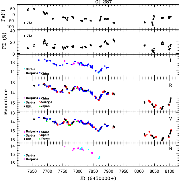
Figure 1: Optical flux and polarization variability light curves of OJ 287 during September 2015 – December 2017. From bottom to top, the panels show B, V, R and I calibrated magnitudes, degree of polarization in R band, and polarization angle in R band, respectively. Different symbols and colors marked inside the panels indicate the data from different telescopes.

In Fig. 1 we present the photometric and polarimetric light curves (LCs) generated from our observing campaign using nine telescopes around the globe during September 2016 – December 2017. We present LCs of the B, V, R, and I bands, as well as the degree of polarization (PD) and polarization angle (PA). The V and R band LCs clearly have the densest observational cadence. The polarimetric observations do not have similarly dense coverage though the most common photometric observations are made in the R band. One can immediately notice that there are several flaring events in the photometric observations in V and R bands, most of which are also seen in I, as well as large changes in the degree of polarization and polarization angle. In the following subsections, we discuss the variability characteristics of the blazar OJ 287 on IDV, STV and LTV timescales, and the nature of the polarization variation.

3.1 Light Curve Analysis Techniques

To quantify the IDV variability results, we use variability detection techniques based on the F-test, the so-called $\chi^{2}$-test, and the Levene test and we describe them briefly in the following subsections. The F-test and $\chi^{2}$-test, which are frerquently employed in studies of AGN variability, assume a normal distribution of the data which is not, in general, true for blazars’ LCs. Thus, we have additionally performed the Levene test, which is a nonparametric variance test. We conservatively claim a LC is variable only if the variability is detected by all three tests. We also calculate the variability amplitude on IDV, STV and LTV timescales. The method used to determine the variability amplitude is also described briefly below.

3.1.1 F-Test

To quantify any IDV of the blazar OJ 287, we originally adopted the commonly used F-Test (de Diego, 2010) and display these results because many other papers in this field have done so, even though it relies on the data displaying a normal distribution. We employ two comparison stars and so define (Gaur et al., 2012a; Agarwal & Gupta, 2015; Gupta et al., 2017a, and the references therein),

$$F_{1}=\frac{Var(BL-star1)}{Var(star1-star2)},F_{2}=\frac{Var(BL-star2)}{Var(star1-star2)}$$ (1)

where (BL $-$ star 1), (BL $-$ star 2), and (star 1 $-$ star 2) are the differential instrumental magnitudes of blazar and standard star 1, blazar and standard star 2, and standard star 1 and standard star 2, respectively, while Var(BL $-$ star 1), Var(BL $-$ star 2), and Var(star 1 $-$ star 2) are the variances of the differential instrumental magnitudes.

Then the relevant $F$ value is the average of $F_{1}$ and $F_{2}$ which is then compared with the critical $F^{(\alpha)}_{\nu_{bl},\nu_{*}}$ value where $\alpha$ is the significance level set for the test while $\nu_{bl}$ and $\nu_{*}$ are the number of degrees of freedom, calculated as ($N-1$), with $N$ the number of measurements. For IDV detection in the LCs, we have done the $F$-test for $\alpha$ values of 0.999 and 0.99, which effectively correspond to $3\sigma$ and $2.6\sigma$ detections, respectively. The null hypothesis (no variability) is discarded if the $F$ value is greater than the critical value, and as usual we claim a LC to be variable if $F>F_{c}(0.99)$ (Agarwal & Gupta, 2015; Gupta et al., 2017a).

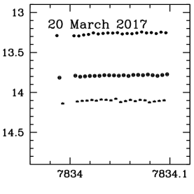
Figure 2: Intraday light curves for OJ 287 in V, R, I filters. Filled triangles, open circles and filled circles represent data in V, R, and I filters, respectively. The X axis is JD (2450000+) and the Y axis is the magnitude in each plot, where observation dates are indicated in each plot.

3.1.2 $\chi^{2}$-Test

To quantify the detection of variability of the blazar we have also used the “so-called” $\chi^{2}$-test (de Diego, 2010). This $\chi^{2}$ statistic is defined as (e.g, Agarwal & Gupta, 2015)

$$\chi^{2}=\sum_{i=1}^{N}\frac{(V_{i}-\overline{V})^{2}}{\sigma_{i}^{2}},$$ (2)

where, $\overline{V}$ is the average magnitude, and $V_{i}$ is the magnitude of $i^{th}$ observation with a corresponding standard error $\sigma_{i}$. We note that this test assumes a Gaussian scatter and constant mean, neither of which are generally seen in blazar LCs, and so these results are included only because this approach has often been used in other studies. It has been determined that the actual measurement errors are larger than the errors indicated by photometry software by a factor of 1.3 $-$ 1.75 (e.g, Gopal-Krishna et al., 2003). So we multiply the errors obtained from the data reductions by a factor of 1.5 (Stalin et al., 2004) to get better estimates of the real photometric errors. The mean value of $\chi^{2}$ is then compared with the critical value $\chi_{\alpha,\nu}^{2}$ where $\alpha$ is the significance level and $\nu=N-1$ is the number of degrees of freedom. A value $\chi^{2}>\chi_{\alpha,\nu}^{2}$ implies the presence of variability.

3.1.3 Levene Test

To quantify the IDV in the LCs of the blazar OJ 287, we also have used the non-parametric Levene test (Brown & Forsythe 1974). It compares the variances of different samples and tests the null hypothesis that all the samples are from populations having equal variances. We calculated the statistics $W_{1}$ and the null hypothesis probability $p_{1}$ for the differential LCs (DLCs) of blazar $-$ Star A and the DLCs of Star A $-$ Star B. Similarly we found $W_{2}$ and $p_{2}$ for the DLCs of blazar $-$ Star B and that of Star A $-$ Star B. A $p$-value greater than 0.01 indicates that the blazar is non-variable with respect to the star. The test statistic, $W$, is defined as

$$W={\frac{(N-k)}{(k-1)}}.{\frac{\sum_{i=1}^{k}N_{i}{(Z_{i.}-Z_{..})}^{2}}{\sum_{i=1}^{k}\sum_{j=1}^{N_{i}}{(Z_{ij}-Z_{i.})}^{2}}}$$ (3)

where
$k$ is the number of different groups to which the sampled cases belong,
$N_{i}$ is the number of cases in the i^th group,
$N$ is the total number of cases in all groups,
$Y_{ij}$ is the value of the measured variable for the j^th case from the i^th group,
$Z_{ij}=|Y_{ij}-{\bar{Y}_{i.}}|$,      ${\bar{Y}_{i.}}|$ is a mean of the i^th group, $|Y_{ij}-{\tilde{Y}_{i.}}|$,      ${\tilde{Y}_{i.}}|$ is a median of the i^th group,
$Z_{i.}={\frac{1}{N_{i}}}{\sum_{j=1}^{N_{i}}}Z_{ij}$ is the mean of the $Z_{ij}$ for group $i$,
$Z_{..}={\frac{1}{N}}{\sum_{i=1}^{k}\sum_{j=1}^{N_{i}}}Z_{ij}$ is the mean of all $Z_{ij}$.

We claimed that the blazar to be non-variable if it is non-variable with respect to both the comparison stars. The values of test statistics and the null hypothesis probabilities are given in Table 3.2. We list a source as certainly variable (Var) only if it satisfies the criteria of all the three tests, i.e. $F$-test, $\chi_{2}$-test, and Levene test.

3.1.4 Amplitude of Variability

The percentage of magnitude and color variations on IDV through LTV time scales can be calculated by using the variability amplitude parameter $A$, which was introduced by Heidt & Wagner (1996) and defined as

$$A=100\times\sqrt{{(A_{max}-A_{min}})^{2}-2\sigma^{2}}(\%)$$ (4)

Here $A_{max}$ and $A_{min}$ are the maximum and minimum values in the calibrated magnitude and color of LCs of the blazar, and $\sigma$ is the average measurement error.

3.2 Intra-day Flux and Color Variability

Table 3.Results of IDV Observations. In the Variable column, Var, and NV represent variable, and non-variable, respectively.
Date Band $N$ $F-$test $\chi^{2}-$test Levene test Variable yyyymmdd $F_{1}$, $F_{2}$, $F$, $F_{c}$(0.99), $F_{c}$(0.999) $\chi^{2}_{1}$, $\chi^{2}_{2}$, $\chi^{2}_{av}$, $\chi^{2}_{0.99}$, $\chi^{2}_{0.999}$ $W_{1}$, $p_{1}$ $W_{2}$, $p_{2}$ 20170220 V 74 0.98, 0.67, 0.83, 1.73, 2.08 75.73, 127.15, 101.44, 104.01, 116.09 4.66e-01, 4.96e-01 6.56e-05, 9.94e-01 NV R 74 1.50, 0.90, 1.20, 1.73, 2.08 59.06, 70.95, 65.00, 104.01, 116.09 5.29e-01, 4.68e-01 2.88e-01, 5.92e-01 NV I 74 1.18, 0.22, 0.70, 1.73, 2.08 320.75, 102.60, 211.67, 104.01, 116.09 5.56e-03, 9.41e-01 1.99e+01, 1.59e-05 NV (V-R) 74 1.00, 0.61, 0.81, 1.73, 2.08 75.76, 94.15, 84.96, 104.01, 116.09 6.03e-02, 8.06e-01 1.30e+00, 2.55e-01 NV (R-I) 74 1.28, 0.32, 0.80, 1.73, 2.08 209.11, 91.13, 150.12, 104.01, 116.09 5.36e-02, 8.17e-01 1.02e+01, 1.71e-03 NV
(This table is available in its entirety in a machine-readable form in the online journal. A portion is shown here for guidance regarding its form and content)

Out of $\sim$175 observing nights during the campaign, we have many nights when multiple image frames were observed in any specific optical band. But to study the optical flux and color variability properties on IDV timescales, we selected only nights with a minimum of ten observations in an optical band by a telescope on a particular observing night, and for plotting the IDV LCs, we decided on a minimum of twenty observations in an optical band by a telescope on a particular observing night. Using these criteria, eleven observing nights qualified for IDV flux and color variability analysis and the results are reported in Table 3, while nine multi-band optical IDV flux LCs are plotted in Fig. 2.

To investigate the flux and color variability on IDV timescales on the above nights, we have used F-test, $\chi^{2}$-test, and Levene test analyses which were briefly explained in sections 3.1.1, 3.1.2, 3.1.3, respectively. Using these tests, the presence or absence of IDV are reported in Table 3 where NV, and Var represent non-variable, and variable natures of LC. It is clearly seen from the plots in Fig. 2 as well as the results reported in Table 3 that, perhaps surprisingly, no genuine IDV was detected in any of the V, R, and I bands IDV LCs in the nine nights of intensive observations that were taken during 20 February 2017 – 3 April 2017. Given the lack of variability in any bands, it is obvious that no color variations were seen on any of these nights on IDV timescales. However, it should be noted that nearly all of these nightly observations were relatively short, spanning between $\sim$2.5 and $\sim$4 hours, and so the chances of detecting IDV were limited.

From the LCs plotted in Figs. 1 and 2, it is can be seen that the blazar OJ 287 was in a fairly bright state during much of these observations. The brightest state detected in the blazar in the outburst in December 2015 was $\sim$13.4 mag in V, 13.0 mag in R, and 12.4 mag in I band (Gupta et al., 2017a). Just from these IDV LCs, we detected OJ 287 in the brightest state on 25 February 2017 when the magnitudes were $\sim$13.9 mag in V, $\sim$13.6 mag in R, and $\sim$13.0 mag in I.

3.3 Short and Long Term Variability

3.3.1 Flux Variability

Significant flux variability of OJ 287 on STV and LTV timescales is evident from the four lower panels of Fig. 1 where the B, V, R, and I band LCs are shown. We have calculated the variability amplitude in B, V, R, and I optical bands and these results are reported in Table 4. Observations in the B band were only carried out using telescopes in Bulgaria and Serbia for a total of sixteen observing nights between 3 January to 3 April 2017, while we have dense observations carried out in V, R, and I bands. We noticed that the faintest level of the blazar in B, V, R, I, bands respectively were 14.921 mag at JD 2457846.39561, 16.164 mag at JD 2458075.58133, 15.670 mag at JD 2458073.96976, and 14.154 mag at JD 2457866.00547. Similarly, the brightest levels we observed of the blazar in the B, V, R, I, bands were 14.126 mag at JD 2457756.53125, 13.582 mag at JD 2457672.36782, 13.179 mag at JD 2457679.620, and 12.720 mag at JD 2457691.29261, respectively. The amplitudes of variation in B, V, R, I bands are 79.5%, 258.2%, 249.1%, 143.4%, respectively, but the smaller values for the B and I bands are explained by the relative paucity of data for them, as all colors are seen to vary together when data were taken for all of them. It can be seen from Fig. 1 that small flares are superimposed on a long term trend. The implications of these results are discussed in Section 4.

Table 4. Results of STV and LTV flux variations.

Band Duration Variable A (percent) yyyy mm dd – yyyy mm dd B 2017 01 03 – 2017 04 26 Var   79.5 V 2016 09 24 – 2017 12 17 Var 258.2 R 2016 09 24 – 2017 12 16 Var 249.1 I 2016 10 09 – 2017 05 24 Var 143.4

Note: Var: Variable; NV: non-variable

Figure 3: Optical color variability light curves covering the entire monitoring period of OJ 287.

3.3.2 Color Variability

Table 5. Color variation with respect to time on short and long timescales.

Color Indices $m_{1}^{a}$ $c_{1}^{a}$ $r_{1}^{a}$ $p_{1}^{a}$ R–I $-$7.011E$-$05    1.063 $-$0.153 2.287E$-$01 B–V $-$1.293E$-$04    1.377 $-$0.059 8.296E$-$01 V–R    2.756E$-$04 $-$1.770    0.634 1.029E$-$14 B–I    2.851E$-$04 $-$0.999    0.156 2.888E$-$01

^a $m_{1}=$ slope and $c_{1}=$ intercept of CI against JD;
$r_{1}=$ Pearson coefficient; $p_{1}=$ null hypothesis probability

Table 6. Color-magnitude dependencies and color-magnitude correlation coefficients on short and long timescales.

Color Indices $m_{2}^{a}$ $c_{2}^{a}$ $r_{2}^{a}$ $p_{2}^{a}$ R–I 7.447E$-$02 $-$0.513 0.487 3.319E$-$08 B–V 2.446E$-$02    0.022 0.097 0.721 V–R 4.093E$-$02 $-$0.209 0.440 1.577E$-$09 B–I 9.934E$-$02 $-$0.174 0.477 0.061

^a $m_{2}=$ slope and $c_{2}=$ intercept of CI against V;
$r_{2}=$ Pearson coefficient; $p_{2}=$ null hypothesis probability

Optical color variations with respect to time (color vs time) and with respect to V band magnitude (color vs magnitude) are plotted in Fig. 3 and Fig. 4, respectively. On visual inspection both the figures show clear color variations. However, it seems there are no consistent systematic trends in the color variations, as shown by straight line fits to the color vs time plot in Fig. 3. However, the color vs magnitude plots in Fig. 4 show bluer-when-brighter (BWB) trends, which are significant for the more frequently measured V–R and R–I colors. Here lines, $Y=mX+c$, are fitted in to each panel in Fig. 3 and Fig. 4. The values of the slopes, $m$, the intercepts, $c$, the linear Pearson correlation coefficients, $r$, and the corresponding null hypothesis probability, $p$, results for color vs time and color vs magnitude are reported in Table 5 and Table 6, respectively.

Figure 4: Optical color-magnitude plots of OJ 287 during our entire monitoring period.

3.3.3 Polarization Variability

In Fig. 1 we plotted optical magnitudes of OJ 287 as well as degree of polarization and polarization angle. It is clear from visual inspection of the figure that the source exhibited large variations in PD and PA as well as overall flux. We noticed the following combinations of variation of flux, degree of polarization, and polarization angle: (i) at $\sim$ JD 2457682 the flare peak at R = 12.957 mag corresponds to a PD of 20%, and PA = 15^∘; (ii) at $\sim$ JD 2457755 the flare peak at R = 13.35 is anti-correlated with PD at only 9% and the PA = $-$35^∘; (iii) at $\sim$ JD 2457790 the flare peak at R = 13.437 mag corresponds to PD = 13% and with PA = $-$63^∘; (iv) the lowest flux state at $\sim$ JD 2458074, with R = 15.670 mag, is anti-correlated, having a high PD $\sim$ 20%, and the PA = $-$25^∘.

Fig. 5 presents the polarization in terms of the normalized Stokes parameters, Q/I vs. U/I, for these data. Here we have used the data taken during JD 2457633 to 2457920, before the $\sim$100 day gap when the blazar could not be observed from the ground. The more limited polarimetric observations taken afterwards have not been used in the analysis. We note there appears to be a systematic change in the polarization fluxes with the polarization angle during the first $\sim$100 days which evinces a clockwise loop-like structure (shown by black to purple points). During the middle part of the observations (red to orange points) there is relatively less change in the Stokes parameters with roughly random variations. However, there is a hint of the beginning of a systematic change over the last 50 days of the observations (yellow points). Over all, the intensity variations in the Q,U–plane are mostly reminiscent of a random-walk, indicating that emission is resulting from different regions with different magnetic field orientations (Moore et al., 1982), throughout the course of observations presented in this study.

3.3.4 Spectral Index Variation and Spectral Energy Distribution

We have dense sampling in V and R bands during our whole observing campaign, so we also calculated spectral indices for for all the epochs where we have V and R bands data on same JD, following Wierzcholska et al. (2015),

$$\alpha_{VR}={0.4\,(V-R)\over\log(\nu_{V}/\nu_{R})}\,$$ (5)

where $\nu_{V}$ and $\nu_{R}$ are effective frequencies of V and R bands, respectively (Bessell et al., 1998). It should be noted that spectral index estimated using this expression differs from the usual index (in $\rm F_{\nu}\propto\nu^{-\alpha}$) by a constant factor related to the zero-point magnitude of the two bands. The spectral index with respect to time, and with respect to V band magnitude are plotted in the bottom and top panels of Fig. 6, respectively. It is clearly seen that there are large variations in $\alpha_{VR}$ between $\sim$1.5 to $\sim$3.2. From Fig. 6 (bottom panel) it is clear that the spectral index systematically increased with respect to time, and from Fig. 6 (top panel), the spectral index increases with respect to increasing V band magnitude, confirming the BWB result. The straight line fitting parameters are given in Table 7.

To further explore the systematic change of the spectral index with time, as well as magnitude, as seen in Fig. 6 we have generated optical SEDs during different optical flux states of the source. We have taken quasi-simultaneous B, V, R, and I band data points at four different states to produce optical SEDs. These states are: during outburst 1 from JD 2457756.5 – 2457757.5; during outburst 2 from JD 2457811.2 – 2457812.5; an intermediate state from JD 2457844.5 – 2457845.5; and a low state from JD 2457867.5 – 2457868.5. Unfortunately we only have data in two bands (V and R) at the lowest flux state of the source on JD 2458074 during this observing campaign and so could not plot an optical SED for it. To generate the SEDs, calibrated magnitudes of OJ 287 in B, V, R, I bands are adjusted for Galactic absorption, with A${}_{B}=$ 0.102 mag, A${}_{V}=$ 0.075 mag, A${}_{R}=$ 0.063 mag, and A${}_{I}=$ 0.045 mag, respectively (Cardelli et al., 1989; Bessell et al., 1998). The SEDs of these four different flux states of the source are plotted in Fig. 7. During the observing campaign there were other periods of strong flaring as well as intermediate or low flux states of the source, but unfortunately we do not have quasi-simultaneous (within a day) observations in at least three optical bands, so those are not considered for making SEDs.

The most striking observation about the optical SEDs during the current period are their relative flatness in the intermediate and low states while there is a slightly rising trend with frequency during outbursts 1 and 2. These are very different compared to the previous optical SEDs of the source so far, which showed a clear declining trend at higher frequencies (Kushwaha et al., 2018a; Gupta et al., 2017a; Kushwaha et al., 2013). The corresponding spectral indices for the four SEDs with respect to V band magnitude, following Eqn. (4), are shown in Figure 8. The indices clearly reflect the variation between the two bands, with indices being lower for harder spectra, as can be seen clearly in the SEDs for the respective states.

4 Discussion

OJ 287 is currently in an enhanced activity phase that started in November 2015 (Kushwaha et al., 2018a; Gupta et al., 2017a; Kushwaha et al., 2018b). The timing of the beginning of this optical enhancement was in accoradance with the inspiraling binary SMBH model (Valtonen et al., 2016, and references therein) which attributes the $\sim 12$ years quasi-periodicity seen in the optical data to the impact of the secondary SMBH on the accretion disk of the primary. Apart from confirming the model predictions, studies and observations of OJ 287 since then have resulted in reporting of many new features in the spectral, temporal, and polarization domains. These include a possible thermal bump in NIR-optical region consistent with primary SMBH accretion disk emission (Kushwaha et al., 2018a), a change in shape of $\gamma$-ray SEDs and shifts in its peak position (Kushwaha et al., 2018a, b), and the first ever detection at very high energies (VHEs, E $>$ 100 GeV; O’Brien, 2017). The work presented here is part of ongoing effort to explore the source activity and features between the two claimed disk impacts via dense follow-up at optical energies. A significant part of the present data has already been presented in another work focusing on MW aspects of the source (Kushwaha et al., 2018b), but that paper was concerned with timescales of interest associated with the MW data cadence. Here, we are focused on investigation on diverse timescales from IDV to LTV which are allowed by the current data and which was not possible with the MW data either due to the low cadence of X-ray and $\gamma$-ray data and/or the lack of good photon statistics for the latter on all the timescales of the optical data considered here.

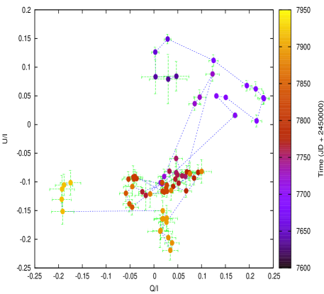
Figure 5: Fractional polarization variations over the course of data presented in this study.

Figure 6: Optical spectral index variation with respect to time and V band magnitude covering the entire monitoring period of OJ 287.

Figure 7: Optical spectral energy distribution (SED) of OJ 287 at different flux state.

The data presented here correspond to the September 2016 – December 2017 period when we have obtained extensive optical photometric and polarimetric monitoring of OJ 287 on a total of $\sim$175 nights from seven different optical telescopes around the globe. Archival data from Steward observatory are also included in our studies. We have searched for flux and color variations on IDV, STV and LTV timescales. We have also searched for color variations with respect to time, color dependence on magnitude, spectral index variation, SED changes, and polarization variations on LTV timescales. Investigation of IDV on 11 nights when we have quasi-simultaneous multi-band (V, R, I) observations showed no significant IDV in fluxes or colors (Table 3.2). On the other hand, on STV and LTV timescales the light curves show strong evidence of major flux changes, with amplitude variations reaching $\sim$250% (Table 3.3.1), including multiple instances of flaring. The lower detected variabilities for the B and I bands are almost certainly due to the lesser amounts of data for them. There is some evolution of the best measured (V$-$R) color with time (Table 3.3.2, Fig. 3) but there are clear systematic variations of color with respect to the V-band measurements (Table 3.3.2, Fig. 4), referred to generally as a BWB trend which is a result of a new non-thermal high-frequency peaked blazar (HBL) component (Kushwaha et al., 2018b).

In the polarization domain, the source reflects the activity seen in the flux variations on similar timescales. Broadly, most of the flux increments are accompanied by an increase in PD which are also associated with frequent changes in the PA by amounts of $\lesssim 50^{\circ}$. The Stokes parameters show a systematic clockwise trend during the first hundred days, followed by an erratic variation and finally a return to a systematic trend towards the end (Fig. 5), indicating the importance of magnetic field changes. We note that the transition from the clockwise trend to the erratic one coincided with the VHE detection and the return to a trend occurred when the source was no longer detectable at those energies (O’Brien, 2017). It should be further noted that PA (after correcting for the $\pm 180^{\circ}$ ambiguity) shows a smooth systematic change of $\sim 125^{\circ}-150^{\circ}$ with small amplitude variations superimposed on it.

Figure 8: Variation of optical spectral index of OJ 287 with V magnitude during two outburst states, an intermediate state, and a low state, where the symbols have the same meaning as in Fig. 7.

The trends and variations seen in the temporal and polarization domains are also reflected in the spectral domain where the VR spectral index shows a systematic change with both V-band magnitude as well as time (Fig. 6). This similar trend with both V-band measurement and flux is reflective of a systematic decline of emission level with time, as can be seen in the light curves. Interestingly, the declining trend is similar to the systematic trend of change in the PA. Further, the flat or uprising optical SEDs suggest that this trend is due to broadband emission. Though there is strong variability with some systematic trends, the variations during the current phase are very different from those seen during our previous observation campaign (Gupta et al., 2017a). Most interestingly, the current data do not display IDV variability despite similar large amplitude variations on LTV and STV timescales, thereby suggesting that the observed variability is governed by regions of larger sizes corresponding to the LTV/STV timescales.

Blazar flux variability on IDV timescales is the most puzzling, and during low states may allow us to probe very close to the central SMBH. IDV in high flux states can be due to evolution of the electron energy density distribution of the relativistic charged particles in which shocks will accelerate relativistic particles in turbulent regions of plasma jets which then cool and lead to a variable synchrotron emission (Marscher et al., 1992; Marscher, 2014; Calafut & Wiita, 2015; O’ Riordan et al., 2017). The most extreme IDV might require acceleration of small regions within the jets to extremely high Lorentz factors (e.g. Giannios et al., 2009). Optical flux variability detected on IDV timescales in low-states can be explained by models based on the accretion disk (e.g., Mangalam & Wiita, 1993; Chakrabarti & Wiita, 1993). Our lack of detection of genuine IDV in any of the 11 densely sampled nights for OJ 287 indicates that during this period the jet emission was quite uniform and that relativistic shock directions did not quickly change with respect to our line of sight. Here we can safely rule out accretion disc based models because source was observed in an overall high flux state, when jet emission must dominate and no flux or color variations were noticed on IDV timescales.

Blazar emission on STV and LTV timescales are dominated by non-thermal jet emission throughout the EM spectrum and can also explain the optical flux and polarization variability on diverse timescales. Shock-in-jet models (e.g. Hughes et al., 1985; Marscher & Gear, 1985; Spada et al., 2001; Graff et al., 2008; Joshi & Böttcher, 2011, and references therein) can explain the general behaviour of flux variability on diverse timescales, while the polarization variability also can be explained by these models (e.g. Marscher et al., 2008; Larionov et al., 2013, and the references therein) particularly when supplemented with turbulence (Marscher, 2014). Changes in the physical parameters set up close to the base of the jet including velocity, electron density, magnetic field, etc., can produce a new shock which can lead to a flaring event when moving along the inhomogeneous relativistic jet. Geometrical effects from jet bending, precession or internal helical structures can lead to changes in the Doppler boosting of the jet emission which can produce a wide variety of flux variations on STV and LTV timescales in blazars (e.g. Camenzind & Krockenberger, 1992; Gopal-Krishna & Wiita, 1992; Pollack et al., 2016).

The four optical SEDs (Fig. 7) during different flux states are almost flat, except for changes in the overall level of emission. In fact, they suggest more emission at the high frequency end, which is very different compared to previous SEDs (Kushwaha et al., 2018a; Gupta et al., 2017a; Kushwaha et al., 2013, and references therein) where normally declining emission is seen. Since any thermal features are not expected to vary appreciably on timescales of days or months, the flatness of the SED and the blue bump emission possibly seen in our previous work Gupta et al. (2017a, see also ()) suggest a contribution from another component in the optical that makes the emission increase at high frequencies (e.g. Kushwaha et al., 2018b). This is clear from the investigation of the broadband SED by Kushwaha et al. (2018b) with OJ 287 SEDs being a sum of LBL, which is the typical SED of OJ 287, and a new HBL spectral component during the high activity states. This new component, peaking in the UV-X-ray region, is responsible for the relative flatness of the SEDs. This is also consistent with the high PD and strong changes of it during these observations, often associated with PA swings and the systematic variation in the fractional polarization suggest the second component to be non-thermal in nature, as also reflected in the strong variability of the optical V-R spectral index on daily timescales (Fig. 6). Although OJ 287 is fundamentally a BL Lac object and has at most very weak emission lines, they may be present at the level of $\sim 10^{42-43}{\rm ergs}^{-1}$, and were apparently seen during the interaction time suggested by the binary SMBH model (Nilsson et al., 2010) and also might be relevant for explaining the overall MW SED shift in the $\gamma$-ray peak (Gupta et al., 2017a; Kushwaha et al., 2018a).

In our flux and polarization monitoring campaign of OJ 287 during 2016 – 2017, we noticed interesting relations between the fluxes, degree of polarization, and polarization angle. There is a systematic swing of $\sim$150^∘ in PA from $\sim$ JD 2457630 – JD 2457850, with a few superimposed short term fluctuations of up to $\sim$50^∘. But during this period the degree of polarization has large variations, from a few percent to over 20 percent. These changes in flux, PD, and PA are quite complex. Interestingly, the fractional polarization shows a systematic clockwise variation during the first 100 days, followed by an essentially random trend and again returning to systematic variation towards the end. It should be noted that the lack of observations before MJD $\sim$ 57650 allow an ambiguity of $\pm 180^{\circ}$ in representation of PA. In our presentation of the PA changes here we chose a smooth variation over a big jump, and so it differs by $180^{\circ}$ to the presentation of some similar data Valtonen et al. (2017). The choice is based on the fact the PD variation seen here is almost always associated with PA change and the fact that the fractional polarization shows both systematic and chaotic trends. Further, in random variation models, a sudden jump of no more than $\pm 90^{\circ}$ is expected (e.g. Marscher, 2014).

In the basic shock-in-jet model, where the shocked region strengthens the ordering of the magnetic field, one can expect a positive correlation between flux and polarization, i.e., an increase in polarization with an increase in flux (Marscher & Gear, 1985; Marscher, 1996; Hagen-Thorn et al., 2008). There are several cases in which blazar flux and degree of polarization show such positive correlations (e.g. Larionov et al., 2008, 2013, 2016, and references therein). Detection of anti-correlated flux and degree of polarization is rare but has been occasionally noticed before (e.g. Gaur et al., 2014). During this observing campaign, we noticed that when the source goes into the lowest flux state, at $\sim$ JD 2457865, the PD is rather high and there is evidence of large swings $\sim$ 70^∘ of the PA. Marscher et al. (2008) gave a generalized model for variation in optical flux, degree of polarization, and polarization angle. The model involves a shock wave leaving the close vicinity of the central SMBH and propagating down only a portion of the jet’s cross section which leads to the disturbance following a spiral path in a jet that is accelerating and becoming more collimated. Larionov et al. (2013) extended the work of (Marscher et al., 2008) and applied this generalized model to multiwavelength variations of an outburst detected in the blazar S5 0716+714. In the model of Larionov et al. (2013), if one changes the bulk Lorentz factor $\Gamma$, even if the remaining parameters (e.g. jet viewing angle, temporal evolution of the outburst, shocked plasma compression ratio $k$, spectral index $\alpha$, and pitch angle of the spiral motion) are kept constant, different combinations in the variations in flux, polarization, and polarization angle can be observed.

5 Summary

We summarize below our results:

$\bullet$ The blazar OJ 287 was in a fairly bright state between September 2016 and December 2017 and several large and small flares were observed in optical bands.
$\bullet$ Using our selection criteria, we had eleven nights during which multi-band intra-day LCs could be extracted but we never saw fast (IDV) variations in flux or color.
$\bullet$ On longer STV and LTV timescales OJ 287 showed large amplitude flux variation in all B, V, R, and I bands with variability in respective band similar to what was found in the previous study (Gupta et al., 2017a).
$\bullet$ Color variations are noticed on STV and LTV timescales in both color vs time and color vs magnitude plots. A bluer-when-brighter trend is noticed between the best sampled V and R bands.
$\bullet$ There are strong variations in degree of polarization and large swings in polarization angle. For most of the time, both flux and polarization show complex variations.
$\bullet$ On two occasions around JD 2457755 and JD 2458074, we noticed that there are strong evidences of anti-correlation in flux with degree of polarization and polarization angle.
$\bullet$ Through plotting the Stokes parameters, we observed that the fractional polarization exhibited a systematic clockwise trend with time during the first hundred days, followed by a more restricted and essentially random variation, and then it appears to revert to a systematic variation. This duration and trend are coincident with the source’s VHE activity (O’Brien, 2017), suggesting a role magnetic field for that activity.

References

- Agarwal & Gupta (2015) Agarwal, A., & Gupta, A. C. 2015, MNRAS, 450, 541
- Agarwal et al. (2015) Agarwal, A., Gupta, A. C., Bachev, R., et al. 2015, MNRAS, 451, 3882
- Andruchow et al. (2003) Andruchow, I., Cellone, S. A., Romero, G. E., Dominici, T. P., & Abraham, Z. 2003, A&A, 409, 857
- Andruchow et al. (2011) Andruchow, I., Combi, J. A., Muñoz-Arjonilla, A. J., et al. 2011, A&A, 531, A38
- Bessell et al. (1998) Bessell, M. S., Castelli, F., & Plez, B. 1998, A&A, 333, 231
- Blandford & Rees (1978) Blandford, R. D., & Rees, M. J. 1978, Phys. Scr, 17, 265
- Brown & Forsythe (1974) Brown, M. B., & Forsythe, A. B. 1974, Journal of the American Statistical Association, 69, 364
- Calafut & Wiita (2015) Calafut, V., & Wiita, P. J. 2015, Journal of Astrophysics and Astronomy, 36, 255
- Camenzind & Krockenberger (1992) Camenzind, M., & Krockenberger, M. 1992, A&A, 255, 59
- Cardelli et al. (1989) Cardelli, J. A., Clayton, G. C., & Mathis, J. S. 1989, ApJ, 345, 245
- Cellone et al. (2007) Cellone, S. A., Romero, G. E., Combi, J. A., & Martí, J. 2007, MNRAS, 381, L60
- Chakrabarti & Wiita (1993) Chakrabarti, S. K., & Wiita, P. J. 1993, ApJ, 411, 602
- de Diego (2010) de Diego, J. A. 2010, AJ, 139, 1269
- Dey et al. (2018) Dey, L., Valtonen, M. J., Gopakumar, A., et al. 2018, ApJ, 866, 11
- Dickel et al. (1967) Dickel, J. R., Yang, K. S., McVittie, G. C., & Swenson, G. W., Jr. 1967, AJ, 72, 757
- Fiorucci & Tosti (1996) Fiorucci, M., & Tosti, G. 1996, A&AS, 116, 403
- Gaur et al. (2010) Gaur, H., Gupta, A. C., Lachowicz, P., & Wiita, P. J. 2010, ApJ, 718, 279
- Gaur et al. (2012a) Gaur, H., Gupta, A. C., & Wiita, P. J. 2012a, AJ, 143, 23
- Gaur et al. (2012b) Gaur, H., Gupta, A. C., Strigachev, A., et al. 2012b, MNRAS, 420, 3147
- Gaur et al. (2012c) Gaur, H., Gupta, A. C., Strigachev, A., et al. 2012c, MNRAS, 425, 3002
- Gaur et al. (2014) Gaur, H., Gupta, A. C., Wiita, P. J., et al. 2014, ApJ, 781, L4
- Gaur et al. (2015) Gaur, H., Gupta, A. C., Bachev, R., et al. 2015, MNRAS, 452, 4263
- Ghisellini et al. (1997) Ghisellini, G., Villata, M., Raiteri, C. M., et al. 1997, A&A, 327, 61
- Giannios et al. (2009) Giannios, D., Uzdensky, D. A., & Begelman, M. C. 2009, MNRAS, 395, L29
- Gopal-Krishna & Wiita (1992) Gopal-Krishna, & Wiita, P. J. 1992, A&A, 259, 109
- Gopal-Krishna et al. (2003) Gopal-Krishna, Stalin, C. S., Sagar, R., & Wiita, P. J. 2003, ApJ, 586, L25
- Goyal et al. (2012) Goyal, A., Gopal-Krishna, Wiita, P. J., et al. 2012, A&A, 544, A37
- Graff et al. (2008) Graff, P. B., Georganopoulos, M., Perlman, E. S., & Kazanas, D. 2008, ApJ, 689, 68
- Gu et al. (2006) Gu, M. F., Lee, C.-U., Pak, S., Yim, H. S., & Fletcher, A. B. 2006, A&A, 450, 39
- Gupta et al. (2004) Gupta, A. C., Banerjee, D. P. K., Ashok, N. M., & Joshi, U. C. 2004, A&A, 422, 505
- Gupta et al. (2008) Gupta, A. C., Fan, J. H., Bai, J. M., & Wagner, S. J. 2008, AJ, 135, 1384
- Gupta et al. (2012) Gupta, A. C., Krichbaum, T. P., Wiita, P. J., et al. 2012, MNRAS, 425, 1357
- Gupta et al. (2016) Gupta, A. C., Agarwal, A., Bhagwan, J., et al. 2016, MNRAS, 458, 1127
- Gupta et al. (2017a) Gupta, A. C., Agarwal, A., Mishra, A., et al. 2017a, MNRAS, 465, 4423
- Gupta et al. (2017b) Gupta, A. C., Mangalam, A., Wiita, P. J., et al. 2017b, MNRAS, 472, 788
- Hagen-Thorn et al. (2008) Hagen-Thorn, V. A., Larionov, V. M., Jorstad, S. G., et al. 2008, ApJ, 672, 40
- Heidt & Wagner (1996) Heidt, J., & Wagner, S. J. 1996, A&A, 305, 42
- Hu et al. (2014) Hu, S.-M., Han, S.-H., Guo, D.-F., & Du, J.-J. 2014, Research in Astronomy and Astrophysics, 14, 719
- Hughes et al. (1985) Hughes, P. A., Aller, H. D., & Aller, M. F. 1985, ApJ, 298, 301
- Joshi & Böttcher (2011) Joshi, M., & Böttcher, M. 2011, ApJ, 727, 21
- Kirk et al. (1998) Kirk, J. G., Rieger, F. M., & Mastichiadis, A. 1998, A&A, 333, 452
- Kushwaha et al. (2013) Kushwaha, P., Sahayanathan, S., & Singh, K. P. 2013, MNRAS, 433, 2380
- Kushwaha et al. (2018a) Kushwaha, P., Gupta, A. C., Wiita, P. J., et al. 2018a, MNRAS, 473, 1145
- Kushwaha et al. (2018b) Kushwaha, P., Gupta, A. C., Wiita, P. J., et al. 2018b, MNRAS, 479, 1672
- Larionov et al. (2008) Larionov, V. M., Jorstad, S. G., Marscher, A. P., et al. 2008, A&A, 492, 389
- Larionov et al. (2013) Larionov, V. M., Jorstad, S. G., Marscher, A. P., et al. 2013, ApJ, 768, 40
- Larionov et al. (2016) Larionov, V. M., Villata, M., Raiteri, C. M., et al. 2016, MNRAS, 461, 3047
- Lehto & Valtonen (1996) Lehto, H. J., & Valtonen, M. J. 1996, ApJ, 460, 207
- Mangalam & Wiita (1993) Mangalam, A. V., & Wiita, P. J. 1993, ApJ, 406, 420
- Marcha et al. (1996) Marcha, M. J. M., Browne, I. W. A., Impey, C. D., & Smith, P. S. 1996, MNRAS, 281, 425
- Marscher & Gear (1985) Marscher, A. P., & Gear, W. K. 1985, ApJ, 298, 114
- Marscher et al. (1992) Marscher, A. P., Gear, W. K., & Travis, J. P. 1992, Variability of Blazars, 85
- Marscher (1996) Marscher, A. P. 1996, Blazar Continuum Variability, 110, 248
- Marscher et al. (2008) Marscher, A. P., Jorstad, S. G., D’Arcangelo, F. D., et al. 2008, Nature, 452, 966
- Marscher (2014) Marscher, A. P. 2014, ApJ, 780, 87
- Miller et al. (1989) Miller, H. R., Carini, M. T., & Goodrich, B. D. 1989, Nature, 337, 627
- Moore et al. (1982) Moore, R. L., Angel, J. R. P., Duerr, R., et al. 1982, ApJ, 260, 415
- Nilsson et al. (2010) Nilsson, K., Takalo, L. O., Lehto, H. J., & Sillanpää, A. 2010, A&A, 516, A60
- O’Brien (2017) O’Brien, S. 2017, arXiv:1708.02160
- O’ Riordan et al. (2017) O’ Riordan, M., Pe’er, A., & McKinney, J. C. 2017, ApJ, 843, 81
- Pollack et al. (2016) Pollack, M., Pauls, D., & Wiita, P. J. 2016, ApJ, 820, 12
- Pursimo et al. (2000) Pursimo, T., Takalo, L. O., Sillanpää, A., et al. 2000, A&AS, 146, 141
- Sillanpaa et al. (1988) Sillanpaa, A., Haarala, S., Valtonen, M. J., Sundelius, B., & Byrd, G. G. 1988, ApJ, 325, 628
- Sillanpaa et al. (1996a) Sillanpaa, A., Takalo, L. O., Pursimo, T., et al. 1996a, A&A, 305, L17
- Sillanpaa et al. (1996b) Sillanpaa, A., Takalo, L. O., Pursimo, T., et al. 1996b, A&A, 315, L13
- Smith et al. (2009) Smith, P. S., Montiel, E., Rightley, S., et al. 2009, arXiv:0912.3621
- Spada et al. (2001) Spada, M., Ghisellini, G., Lazzati, D., & Celotti, A. 2001, MNRAS, 325, 1559
- Stalin et al. (2004) Stalin, C. S., Gopal Krishna, Sagar, R., & Wiita, P. J. 2004, Journal of Astrophysics and Astronomy, 25, 1
- Stocke et al. (1991) Stocke, J. T., Morris, S. L., Gioia, I. M., et al. 1991, ApJS, 76, 813
- Valtonen et al. (2008a) Valtonen, M. J., Lehto, H. J., Nilsson, K., et al. 2008a, Nature, 452, 851
- Valtonen et al. (2008b) Valtonen, M., Kidger, M., Lehto, H., & Poyner, G. 2008b, A&A, 477, 407
- Valtonen et al. (2009) Valtonen, M. J., Nilsson, K., Villforth, C., et al. 2009, ApJ, 698, 781
- Valtonen et al. (2010) Valtonen, M. J., Mikkola, S., Merritt, D., et al. 2010, ApJ, 709, 725
- Valtonen et al. (2016) Valtonen, M. J., Zola, S., Ciprini, S., et al. 2016, ApJ, 819, L37
- Valtonen et al. (2017) Valtonen, M., Zola, S., Jermak, H., et al. 2017, Galaxies, 5, 83
- Villforth et al. (2010) Villforth, C., Nilsson, K., Heidt, J., et al. 2010, MNRAS, 402, 2087
- Wagner & Witzel (1995) Wagner, S. J., & Witzel, A. 1995, ARA&A, 33, 163
- Wierzcholska et al. (2015) Wierzcholska, A., Ostrowski, M., Stawarz, Ł., Wagner, S., & Hauser, M. 2015, A&A, 573, A69
- Woo & Urry (2002) Woo, J.-H., & Urry, C. M. 2002, ApJ, 579, 530
- Zhang et al. (2018) Zhang, H., Li, X., Guo, F., & Giannios, D. 2018, ApJ, 862, L25