Thorough evaluation of GHZ generation protocols using conference key agreement

Abstract

The generation of GHZ states in quantum networks is a key element for the realization of several quantum information tasks. Given the complexity of the implementation of such generation, it is not easy to find an unambigous proof for an optimal protocol. Motivated by recent improvements in NV center manipulation, we present and compare an extensive list of protocols for generating GHZ states using realistic parameters. Furthermore, in order to establish the goodness of the various protocols, we test them on a specific application, i.e. conference key agreement. We show that for an high number of nodes the best protocol is one presented here for the first time.

I Introduction

The generation and storage of GHZ states GHZ89 in a distributed fashion would allow the realization of several quantum tasks in quantum networks, namely reducing communication complexity Buhrman01 ; Buhrman10 , distributed quantum computation Cleve97 ; Grover97 ; Li15 ; Li16 , quantum repeaters of second and third generation Muralidharan16 ; Gottesman99 ; Muralidharan14 ; Munro12 , and atomic clock synchronization Komar14 . But it is in quantum cryptography that GHZ states find their most important applications. Examples of that are quantum secret sharing Hillery99 , anonimous state transfer Christandl05 , and conference key agreement (CKA) Epping16 . From the experimental point of view, impressive improvements have been done in generating bipartite entanglement in a distributed fashion with NV centers Bernier13 ; Gao15 , and trapped ions Hucul15 ; Delteil16 . It is now possible to generate bipartite entangled states reaching very high fidelities enabling to successfully test nonlocality Hensen15 . However, little effort has been done so far for the realization of multipartite entanglement. This is because the high fidelities reached for bipartite entanglement have been realized at the cost of very low generation rates. Unfortunately, working with several parties could only worsen this result. In a previous work Caprara17 , we have investigated how to generate GHZ states in a quantum network through one single measurement on ancillary qubits. There, we have shown that there is an intrinsic bound on the achievable success probability when one wants to generate entanglement in a distributed fashion in one single round. In the case of bipartite entanglement, this bottleneck can be overcome through the use of distillation procedures like the extreme-photon-loss (EPL) protocol Li15 , that has recently been experimentally realized Kalb17 . Unfortunately, this happens at the cost of decreasing the fidelity. Hence, it is of primary importance to investigate different protocols in order to get the best compromise between fidelity and generation rate. This task is not easely doable since it is not clear how to evaluate the goodness of such a compromise.

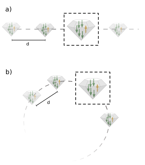
Figure 1: Quantum network architectures. Each node is constituted by a NV center where one electronic spin (yellow arrow) and up to five nuclear spins (green arrows) can be stored. In the case of a) (b)) a linear (circular) architecture is represented. In both cases the nodes are distributed at a fixed distance $d$.

An approach to the issue is to compare the different protocols in terms of a specific application and to evaluate the total application rate. Since the application rate depends both on the generation rate and the goodness of the multipartite state, it constitutes an unambigous parameter for selecting a successful protocol. A recent work Ribeiro17 analyzes conference key agreement (CKA) in presence of losses and gives an expression for the asymptotic rate in a fully device-independent scenario. In this paper, we investigate how to generate GHZ states between nearby nodes through distillation procedures, error correction, and linear optics.

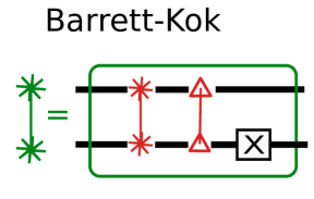
Figure 2: Barrett-Kok circuit. An EPR pair is generated between two distant nodes through two successful consecutive measurements on ancillary modes. Finally, an X rotation is applied on one qubit, passing from $\lvert\Psi^{+}\rangle$ to $\lvert\Phi^{+}\rangle$. The two red star symbol (two red triangle symbol) represents a successful Bell measurement over ancillary modes entangled with the $\lvert 0\rangle$-levels ($\lvert 1\rangle$-levels).

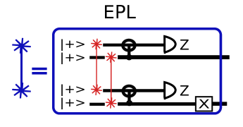
Figure 3: EPL circuit. An EPR pair is generated between distant nodes through a distillation procedure. Firstly, two non-maximally entangled pairs are generated through two distinct successful Bell measurements. Secondly, CNOT and measurements are performed locally. Finally, an X rotation is applied on one qubit.

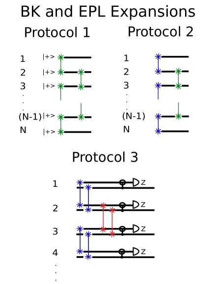
Figure 4: Circuit diagrams for the linear protocols that are BK/EPL expansions. Protocol 1: the BK protocol (two green star symbols) is applied in two subsequently time steps between neighbouring nodes. Protocol 2: $N/2-1$ successful Barrett-Kok procedures are performed between $N/2$ EPL pairs. Protocol 3: a distillation procedure (CNOT and local measurement) is applied on two non-maximally multipartite entangled states.

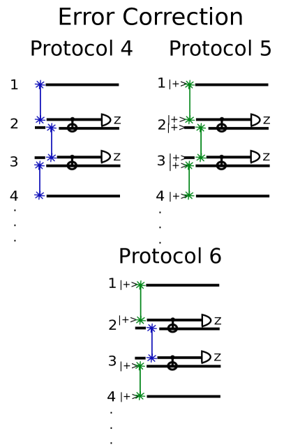
Figure 5: Circuit diagrams for the linear protocols that exploit bipartite entanglement and error correction. Protocol 4: CNOTs and measurements are locally applied over $(N-1)$ EPL pairs. Protocol 5: CNOTs and measurements are locally applied over $(N-1)$ Barrett-Kok pairs. Protocol 6: an error correction procedure is performed over $N/2$ Barrett-Kok and $(N/2-1)$ EPL pairs.

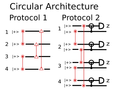
Figure 6: Circuit diagrams for circular protocols 1 and 2. Protocol 1: $N$ successful measurements are performed over $N$ nodes in a circle. Protocol 2: a distillation procedure consisting on a CNOT and a measurement in each node, is performed over non-maximally entangled pairs.

The system we envision is composed by N nodes, each one containing up to five qubits, even though at most two are necessary. One and two qubit logical operations can be performed locally. The nodes interact between each other through ancillary photonic modes that are entangled with the qubit levels. Since the implementable protocols depend on the configuration the nodes are arranged in, we consider two different architectures, or along a line, or along a circle. Notice that in the latter configuration each node is close enough to only two nodes, such that it is easy for it to generate an entangled pair with each one of them. Here, we first present and compare eight protocols in terms of fidelity and generation rate in a realistic scenario, namely NV centers. For linear architectures, we present six protocols, regrouped in two subsets. One set (Fig. 4) is composed by protocols that consist in applying repeatedly the Barrett-Kok (BK)Barrett05 ; Lim05 and EPL Li15 bipartite techniques. The other set (Fig. 5) is composed by all the protocols where, firstly, maximally entangled pairs are realized between nearby nodes, and, secondly, error correction is used to generate the final multipartite entangled state. This approach has already been proposed by Komar, et al. Komar16 . We, here, further investigate this possibility varying the way the maximally entangled pairs are generated. For a circular architecture, we present two protocols (Fig. 6), one already envisioned in Caprara17 , and a new distillation one. As a term of comparison, we use the minimal required fidelity for asymptotic CKA Ribeiro17 . We, furthermore, derive the total asymptotic rate for CKA for all the reasonable protocols. The results show that there is a clear trend as the number of nodes increases. Indeed, for high number of nodes, the circular protocols reveal to be dozens of orders of magnitude faster than the linear protocols. The cause of that has to be sought in the possibility of connecting each node with other two nodes. As a consequence the number of probabilistic operations necessary to generate maximally entangled states is highly reduced. One ends up with GHZ states low decohered and high generation rates.

II Modeling NV centers and losses

In order to evaluate the different protocols in presence of loss and decoherence we need to contextualize them choosing a specific system. NV centers are the perfect candidates for such protocols. In this section, we describe the error model for NV centers. In the system that we envision, each node is constituted by an NV center. For the sake of simplicity, we assume the number of nodes $N$ to always be even. For each NV center we have at our disposal several spins, namely an electronic spin and up to five nuclear spins Reiserer16 . Only the electronic spin can directly be manipulated and any operation on nuclear spins is performed through the electronic spin. We assume that any operation on a single nuclear spin is not affected by decoherence. When one access the electronic spin, the nuclear spins undergo dephasing due to hyperfine interaction between the first and the second ones Reiserer16 . The expression for a dephasing channel on a density matrix $\rho$ is the following

$$D_{\text{deph}}(\rho)=\frac{1+\lambda}{2}\rho+\frac{1-\lambda}{2}\sigma_{z}\rho\sigma_{z},$$ (1)

where $\lambda=e^{-an}$ quantifies the noise. In the expression of $\lambda$, $n$ is the number of attempts that have been performed on the electronic spin, while $a$ depends both on the attempt of accessing the other qubit in the same node and the time required for performing the specific operations. The expression for $a$ is $a=a_{0}+a_{1}t_{\text{step}}$Rozpedek17 , where $a_{0}=\frac{1}{2000}$ per attempt, $a_{1}=\frac{1}{3}$ per second due to the storing time, and $t_{\text{step}}$ is the time required to perform the specific step of the protocol. When the decohering nuclear spin is not stored in a NV center, where one is operating on the electronic spin, $a$ takes the form $a=a_{1}t_{\text{step}}$. Each $\lambda$ factor must be averaged over the number of attempts, i.e.

$$\begin{split}\langle\lambda\rangle&=\frac{\sum_{n=0}^{\infty}\left[P_{\text{succ}}(1-P_{\text{succ}})^{n}e^{-an}\right]}{\sum_{n=0}^{\infty}\left[P_{\text{succ}}(1-P_{\text{succ}})^{n}\right]}\\ &=\frac{P_{\text{succ}}e^{a}}{e^{a}-1+P_{\text{succ}}},\end{split}$$ (2)

where $P_{\text{succ}}$ is the probability of success per attempt of the specific operation, and the sums of the series are performed over all the attemps. In all the protocols the terms outside the space $\{\lvert 0\rangle^{\otimes N},\lvert 1\rangle^{\otimes N}\}$, where N is the number of nodes, are nullified. As a consequence, the final density matrix $\rho_{\text{final}}$ takes the form

$$\rho_{\text{final}}=\frac{1}{2}\left(\begin{array}[]{ccccc}1&0&\cdots&0&\langle\lambda\rangle_{\text{tot}}\\ 0&&&&0\\ \vdots&&\makebox(0.0,0.0)[]{\text{\huge 0}}&&\vdots\\ 0&&&&0\\ \langle\lambda\rangle_{\text{tot}}&0&\cdots&0&1\end{array}\right),$$ (3)

where $\langle\lambda\rangle_{\text{tot}}=\prod_{i}\langle\lambda_{i}\rangle$ is the product between all the factors $\langle\lambda_{i}\rangle$ that cause decoherence during the protocol on all the spins. The losses in the optical setup are represented through the total transmittivity $\eta$, i.e.

$$\eta=\eta_{D}p_{\text{fc}}p_{\text{out}}10^{-\frac{\alpha d}{L_{0}}},$$ (4)

where $\eta_{D}=1$ is the detector efficiency, $p_{\text{fc}}=0.3$ is the frequency conversion efficiency, $p_{\text{out}}=0.3$ is the NV outcoupling efficiency, $L_{0}=20$ km is the attenuation length of the fibres vanDam17 , and $d$ is the distance between two neighbouring nodes.

III Fidelity and generation rate

In order to estimate the goodness of each protocol it is useful to evaluate the fidelity of the final state for each protocol with the GHZ state. We, furthermore, compare the fidelities with the minimal required fidelity for CKA with the protocol presented in Ribeiro17 . In the aforementioned work, the system is affected by depolarizing noise, i.e.

$$D_{\text{depol}}(\rho^{\text{qubit}})=(1-p)\rho^{\text{qubit}}+p\operatorname{Tr}(\rho^{\text{qubit}})\frac{\mathbb{1}}{2},$$ (5)

where $p$ is the noise that affects each spin. The expression for the fidelity with the GHZ state (see appendix VI) is

$$F_{\text{CKA}}=\frac{1}{2}\left(1-\frac{p}{2}\right)^{N}+\frac{(1-p)^{N}}{2}+\frac{1}{2}\left(\frac{p}{2}\right)^{N},$$ (6)

where $N$ is the number of nodes. The maximal $p$ for each $N$ in order to achieve a positive CKA rate is numerically evaluated in Ribeiro17 . The fidelity between a GHZ state and a state in the form of Equ. (3) is

$$F=\frac{1+\langle\lambda\rangle_{\text{tot}}}{2}.$$ (7)

the details of both $\langle\lambda\rangle_{\text{tot}}$ and generation rate for all the protocols are given in appendix VII and VIII.

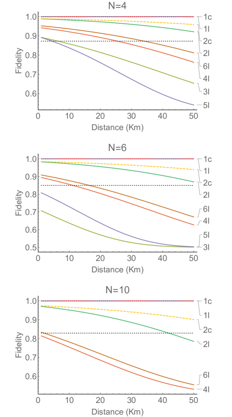
Figure 7: Fidelity for $N=4$, $6$, and $10$ for the different protocols. The fidelity of the final state with the GHZ as a function of the distance is plotted for all the protocols. The black line represents the minimal fidelity necessary to implement the CKA device-independently. For $N=10$, linear protocol 3 and 5 have been omitted.

The fidelities for $N=4$, $N=6$ and $N=10$ as a function of the distance between the nodes are plotted in Figs. 7. The minimal fidelity for CKA is the dashed black line. For $N=4$, all the protocols are above the threshold for some range. However, linear protocols do perform worse. Specifically, it seems that error correcting protocols present more decoherence. Increasing the number of nodes, linear protocols 3,4,5, and 6 become useless. Hence, only linear and circular protocols 1s and 2s are resistant to decoherence. The rates for only the successful protocols as a function of the distance are plotted in Figs. 8 for $N=4$, $N=6$ and $N=10$. From the plots, it is unclear what protocol is the most advantageous among the several.

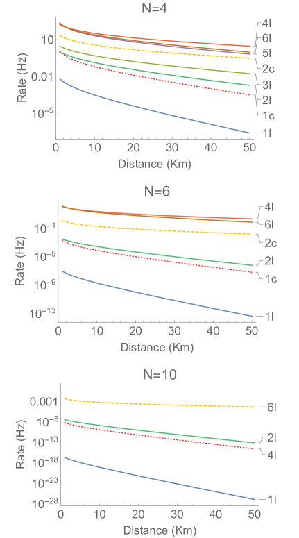
Figure 8: Generation rate for $N=4$, $6$, and $10$ for the different protocols. The rate of generation $R_{\text{GHZ}}$ as a function of the distance is plotted for all the protocols that have fidelity above the thresholds.

The linear protocols 4, 5, and 6 are not usable when the distance between nodes is above around 30 km. However, the latest consideration does not exclude that they are the most suitable for a short distance. Indeed, the linear protocols 4, 5, and 6 have better rates than the others, but have high decoherence. In the next section, we are going to discuss how to overcome this difficulty using the CKA asymptotic key rate.

IV Conference key agreement rate

In this section, we calculate the CKA asymptotic key rate starting from the expression of the fidelity and generation rate for a given protocol, and analyze it as a function of the distance between the nodes. The expression for the CKA asymptotic key rate is Ribeiro17

$$\tilde{R}_{\text{CKA}}=1-h\left(\frac{1}{2}+\frac{1}{2}\sqrt{\frac{MK_{N}^{2}}{2^{N-2}}-1}\right)-h(Q),$$ (8)

where $h(\cdot)$ is the binary entropy, $MK_{N}$ is the MABK value Mermin90 ; Ardehali92 ; Belinski93 in the N-partite case for the dephased GHZ state, and $Q$ is the quantum bit error rate (QBER). The QBER is given by the probability of getting a flip error. Hence, in the case of $\rho_{\text{final}}$ the QBER is 0, i.e. $Q=0$. We have then,

$$h(Q=0)=\lim_{Q\rightarrow 0}\left[Q\log_{2}Q-(1-Q)\log_{2}(1-Q)\right]=0.$$ (9)

It can be numerically proven that the $MK_{N}$ violation for $\rho_{\text{final}}$ (Equ. (3)) is $2^{\frac{N-1}{2}}\langle\lambda\rangle_{\text{tot}}$. Thus, the CKA asymptotic key rate becomes

$$\tilde{R}_{\text{CKA}}=1-h\left(\frac{1}{2}+\frac{1}{2}\sqrt{2\langle\lambda\rangle_{\text{tot}}^{2}-1}\right).$$ (10)

The rate in Equ. (10) must be multiplied by the GHZ generation rate $R_{\text{GHZ}}$, i.e.

$$R_{\text{CKA}}=\tilde{R}_{\text{CKA}}R_{\text{GHZ}}.$$ (11)

The results for $N=4$, $6$ and $10$ as a function of the distance are shown in Figs. 9.

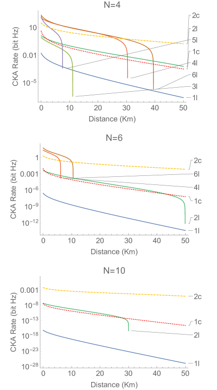
Figure 9: Application rate for $N=4$, 6, and 10 for different protocols. The CKA rate is plotted as a function of the distance between two nodes for all the protocols that have a sufficient high fidelity. In several cases, CKA rates suddenly drops to 0 when the dephased GHZ state does not anymore violate the MABK inequality.

For 4 and 6 nodes, the error correcting protocols are the most effective for short ranges ($\approx 40$ km and $20$, respectively). For longer ranges, the circular protocol 2 is the fastest one. Concerning the linear protocols, albeit extremely slow, protocols 1 and 2 still perform.

V Conclusion

In this article, we have reported of a detailed study of several protocols for GHZ generation in a quantum network composed by NV centers. We evaluate the effectiveness of these protocols through the calculation of three values, the fidelity, the generation rate, and a figure of merit that combines both fidelity and generation rate, i.e. the asymptotic CKA rate. Indeed, the fidelity and the generation rate are common and widespread measures of the goodness of any protocol and are easy to read and interpret for a great audience. However, we found that such a complex protocol analysis was incomplete, since the two observables vary independently from each other. Testing protocols over a specific application is not new Nickerson14 . What it is new is the extensiveness of the study, both in the variety of the protocols and the decoherence analysis. Concerning the protocols, some of them have been proposed in recent papers Caprara17 ; Komar16 , some have partially been readapted from previous work Barrett05 ; Lim05 ; finally, only circular protocol 2 is completely new. In any case, they entirely cover the approaches so-far envisioned. Concerning the decoherence analysis, our study differs from all the previous ones, since we have considered a realistic scenario, including the decoherence due to waiting time, that reveils to be critical for the effectiveness of the protocols. The results show that as the number of nodes increases, the best protocol is the one proposed for the first time, here. Our interpretation is that, for the new protocol, the time required for the generation of the intermediate entanglement is extremely low, resulting in few decoherence and relatively high generation rate. However, this is possible only for circular architectures and not linear. Therefore, there are doubtless cases when such a protocol can not be implemented because of the network architecture. In this instance, the best protocol is the linear protocol 1, i.e. a protocol consisting of only one round. Moreover when one focus only on linear architectures, surprisingly, only protocols 1 and 2, protocols with very low rates, are available. On the contrary, all the protocols that extensively use distillation and error correction result to be too noisy for CKA. This counterintuitive result is a direct consequence of the decoherence due to the waiting times between bipartite entanglement generation and the following step. Concerning the decoherence analysis, few remarks have to be done. First, it is important to stress that the system might encounter other decoherence processes, for example depolarizing channels. Nevertheless, we notice that we have compared the fidelities with a trademark fidelity computed for depolarizing noise. In that frame, some protocols showed to not have enough good fidelities for some specific distances. We have found the same result in section IV for the same distances analyzing the CKA rate. It is, then, our understanding that the qualitative results do not significantly change depending on the decoherence nature. Secondly, we do aknowledge that few sources of decoherence and imperfections have not been taken into account. Examples are the detector dark counts, and the unfidelities of one, two qubit logical ports. Nevertheless, they seem to be of lower impact on the results and, then, do not affect our conclusion on the analysis. Further research should be in two directions. the first is to test how well other quantum information tasks that exploit multipartite entanglement perform with these protocols. The second is to focus on finding new alternative linear protocols that can improve the applications performance. We want, then, to conclude saying that our study represents a detailed and realistic work on GHZ generation that reveils some misconceptions on the main network noise sources and proposes a new promising protocol.

Aknowledgements
We thank Jérémy Ribeiro, Filip Rozpȩdek, and Stephanie Wehner for fruitful discussions.

Appendix

VI Calculation of the fidelity for depolarizing noise

In Ribeiro17 , a depolarizing channel $D_{\text{depol}}(\rho^{\text{qubit}})$ acts on each qubit. The expression of $D_{\text{depol}}(\rho^{\text{qubit}})$ is

$$D_{\text{depol}}(\rho^{\text{qubit}})=(1-p)\rho^{\text{qubit}}+p\operatorname{Tr}(\rho^{\text{qubit}})\frac{\mathbb{1}}{2},$$ (12)

where $\rho^{\text{qubit}}$ is the density matrix of a single qubit and $p$ is the depolarizing factor. The total state $\tilde{\rho}_{\text{final}}$ is, then

$$\tilde{\rho}_{\text{final}}=D^{\otimes N}(\lvert\text{GHZ}\rangle\langle\text{GHZ}\rvert_{N}),$$ (13)

where $N$ is the number of nodes. We need to rewrite $\tilde{\rho}_{\text{final}}$ in a more explicit way, i.e.

$$\begin{split}\tilde{\rho}_{\text{final}}&=(1-p)^{N}\lvert\text{GHZ}\rangle\langle\text{GHZ}\rvert_{N}\\ &+\sum_{S\in\{0,1\}^{N},S\not=\vec{0}}\operatorname{Tr}_{S}(\lvert\text{GHZ}\rangle\langle\text{GHZ}\rvert_{N})\\ &\otimes\frac{\mathbb{1}}{2^{W_{H}(S)}}(1-p)^{N-W_{H}(S)}p^{W_{H}(S)}\\ &=(1-p)^{N}\lvert\text{GHZ}\rangle\langle\text{GHZ}\rvert_{N}\\ &+\sum_{S\in\{0,1\}^{N},S\not=\vec{0}}\frac{\lvert 0\rangle\langle 0\rvert^{N-W_{H}(S)}+\lvert 1\rangle\langle 1\rvert^{N-W_{H}(S)}}{2}\\ &\otimes\frac{\mathbb{1}}{2^{W_{H}(S)}}(1-p)^{N-W_{H}(S)}p^{W_{H}(S)},\end{split}$$ (14)

where $W_{H}(S)$ is the hamming weight of the vector $S$. The fidelity with the $\lvert\text{GHZ}\rangle$ as a function of $p$ is

$$\begin{split}F&=\operatorname{Tr}(\lvert\text{GHZ}\rangle\langle\text{GHZ}\rvert_{N}\tilde{\rho}_{\text{final}})\\ &=(1-p)^{N}+\left(\frac{p}{2}\right)^{N}\\ &+\frac{1}{2}\sum_{S\in\{0,1\}^{N},S\not=\vec{0},\vec{1}}\frac{1}{2^{W_{H}(S)}}(1-p)^{N-W_{H}(S)}p^{W_{H}(S)}\\ &=(1-p)^{N}+\left(\frac{p}{2}\right)^{N}+\frac{1}{2}\sum_{k=1}^{N-1}\binom{N}{k}(1-p)^{N-k}\left(\frac{p}{2}\right)^{N}\\ &=\frac{1}{2}\left(1-\frac{p}{2}\right)^{N}+\frac{(1-p)^{N}}{2}+\frac{1}{2}\left(\frac{p}{2}\right)^{N}.\end{split}$$ (15)

$p$ is numerically evaluated in Ribeiro17 .

VII Calculation of the dephasing factors and fidelities

In this section, we first derive twelve dephasing terms $\langle\lambda_{i}\rangle$ intervening during the protocols in single nodes. Afterwards, we report the expressions of all the fidelities for the different protocols. In the main text, we derived the expression for $\langle\lambda_{i}\rangle$, i.e.

$$\langle\lambda_{i}\rangle=\frac{P^{i}_{\text{succ}}e^{a^{i}}}{e^{a^{i}}-1+P^{i}_{\text{succ}}}.$$ (16)

Each $\langle\lambda_{i}\rangle$, that depends on $P^{i}_{\text{succ}}$ and $a^{i}$, gives account of the dephasing of a single nuclear spin involved in the protocols. Concerning the expression of $a^{i}$, it depends on the two terms $a_{0}$ and $a_{1}$. $a_{1}$ gives count of the decoherence of the nuclear spin while it has to be stored, while $a_{0}$ represents the decoherence caused by each attempt of access on the electronic spin in the same NV center. As a consequence, $a_{0}$ is not present in $a^{i}$ when the decohering nuclear spin is not in a NV center whose electronic spin is manipulated. In Table 1, we report the different processes that occur during the protocols, the dephasing processes connected to them, the $P^{i}_{\text{succ}}$, and the $a^{i}$. The $\langle\lambda_{i}\rangle$ are reported below,

$$\langle\lambda_{1}\rangle=\frac{P^{1}_{\text{succ}}e^{a_{0}+a_{1}t_{1}}}{e^{a_{0}+a_{1}t_{1}}+P^{1}_{\text{succ}}-1},$$ (17)

$$\langle\lambda_{2}\rangle=\prod_{l=1}^{\frac{N}{2}-1}\left(\frac{P^{2}_{\text{succ}}e^{a_{1}t_{2}}}{H_{l}\left(e^{a_{1}t_{2}}+\frac{P^{2}_{\text{succ}}}{H_{l}}-1\right)}\right)^{2},$$ (18)

$$\langle\lambda_{3}\rangle=\frac{P^{3}_{\text{succ}}e^{a_{0}+a_{1}t_{1}}}{e^{a_{0}+a_{1}t_{1}}+2^{2-N}P^{3}_{\text{succ}}-1},$$ (19)

$$\langle\lambda_{4}\rangle=\prod_{l=1}^{\frac{N}{2}}\left(\frac{P^{2}_{\text{succ}}e^{a_{0}+a_{1}t_{2}}}{\left(H_{\frac{N}{2}}-H_{l-1}\right)\left(e^{a_{0}+a_{1}t_{2}}+\frac{P^{2}_{\text{succ}}}{H_{\frac{N}{2}}-H_{l-1}}-1\right)}\right)^{2},$$ (20)

$$\langle\lambda^{\prime}_{4}\rangle=\prod_{l=1}^{\frac{N}{2}-1}\left(\frac{P^{2}_{\text{succ}}e^{a_{1}t_{2}}}{H_{l}\left(e^{a_{1}t_{2}}+\frac{P^{2}_{\text{succ}}}{H_{l}}-1\right)}\right)^{2},$$ (21)

$$\langle\lambda_{5}\rangle=\prod_{l=1}^{\frac{N}{2}-2}\left(\frac{P^{2}_{\text{succ}}e^{a_{1}t_{2}}}{H_{l}\left(e^{a_{1}t_{2}}+\frac{P^{2}_{\text{succ}}}{H_{l}}-1\right)}\right)^{2},$$ (22)

$$\langle\lambda_{6}\rangle=\left(\frac{P^{2}_{\text{succ}}e^{a_{1}t_{2}}}{H_{\frac{N}{2}-1}\left(e^{a_{1}t_{2}}+\frac{P^{2}_{\text{succ}}}{H_{\frac{N}{2}-1}}-1\right)}\right)^{2},$$ (23)

$$\langle\lambda_{7}\rangle=\prod_{l=1}^{\frac{N}{2}-1}\left(\frac{P^{2}_{\text{succ}}e^{a_{0}+a_{1}t_{2}}}{\left(H_{\frac{N}{2}-1}-H_{l-1}\right)\left(e^{a_{0}+a_{1}t_{2}}+\frac{P^{2}_{\text{succ}}}{H_{\frac{N}{2}-1}-H_{l-1}}-1\right)}\right)^{2},$$ (24)

$$\langle\lambda^{\prime}_{7}\rangle=\prod_{l=1}^{\frac{N}{2}-2}\left(\frac{P^{2}_{\text{succ}}e^{a_{1}t_{2}}}{H_{l}\left(e^{a_{1}t_{2})}+\frac{P^{2}_{\text{succ}}}{H_{l}}-1\right)}\right)^{2},$$ (25)

$$\langle\lambda_{8}\rangle=\prod_{l=1}^{\frac{N}{2}-1}\left(\frac{P^{8}_{\text{succ}}e^{a_{0}+a_{1}t_{1}}}{\left(H_{\frac{N}{2}-1}-H_{l-1}\right)\left(e^{a_{0}+a_{1}t_{1}}+\frac{P^{8}_{\text{succ}}}{H_{\frac{N}{2}-1}-H_{l-1}}-1\right)}\right)^{2},$$ (26)

$$\langle\lambda^{\prime}_{8}\rangle=\prod_{l=1}^{\frac{N}{2}-2}\left(\frac{P^{8}_{\text{succ}}e^{a_{1}t_{1}}}{H_{l}\left(e^{a_{1}t_{1}}+\frac{P^{8}_{\text{succ}}}{H_{l}}-1\right)}\right)^{2},$$ (27)

$$\langle\lambda_{9}\rangle=\prod_{l=1}^{\frac{N}{2}-1}\left(\frac{P^{8}_{\text{succ}}e^{a_{1}t_{1}}}{H_{l}\left(e^{a_{1}t_{1}}+\frac{P^{8}_{\text{succ}}}{H_{l}}-1\right)}\right)^{2},$$ (28)

$$\langle\lambda_{10}\rangle=\left(\frac{P^{8}_{\text{succ}}e^{a_{1}t_{1}}}{H_{\frac{N}{2}-1}\left(e^{a_{1}t_{1}}+\frac{P^{8}_{\text{succ}}}{H_{\frac{N}{2}-1}}-1\right)}\right)^{2},$$ (29)

$$\langle\lambda_{11}\rangle=\prod_{l=1}^{\frac{N}{2}-1}\left(\frac{P^{1}_{\text{succ}}e^{a_{1}t_{1}}}{H_{l}\left(e^{a_{1}t_{1}}+\frac{P^{1}_{\text{succ}}}{H_{l}}-1\right)}\right)^{2},$$ (30)

$$\langle\lambda_{12}\rangle=\prod_{l=1}^{\frac{N}{2}}\left(\frac{P^{1}_{\text{succ}}e^{a_{0}+a_{1}t_{1}}}{\left(H_{\frac{N}{2}}-H_{l-1}\right)\left(e^{a_{0}+a_{1}t_{1}}+\frac{P^{1}_{\text{succ}}}{H_{\frac{N}{2}}-H_{l-1}}-1\right)}\right)^{2},$$ (31)

where $H_{m}$ is the harmonic number ($H_{m}=\sum_{n=1}^{m}\frac{1}{n}$).

	Decoherence Process	$P^{i}_{\text{succ}}$	$t_{\text{step}}$
1	Excitation of two electronic spins ($\lvert 0\rangle$-levels)
	and Bell measurement between the	$\frac{1}{4}(4-\eta)\eta$	$\frac{d}{c}+t_{\text{prep}}$
	photonic modes. Decoherence on a nuclear
	spin in the same NV center.
2	Collective dephasing of the EPL pairs
	already generated while waiting for the	$\frac{\eta}{2(4-\eta)}$	$2\left(\frac{d}{c}+t_{\text{prep}}\right)+P^{1}_{\text{succ}}(S_{g}+t_{\text{CNOT}})$
	generation of the remaining pairs
	from 1 to $N/2-1$
3	Excitation of $\frac{N}{2}$ electronic spins ($\lvert 0\rangle$-levels)	$\frac{(4-\eta)\eta^{\frac{N}{2}-1}\left(\eta^{2}-4\eta+8\right)^{\frac{N}{4}-1}}{2^{N-2}}$	$\frac{d}{c}+t_{\text{prep}}$
	and $\frac{N}{2}-1$ Bell measurements between the
	photonic modes. Decoherence on a nuclear
	spin in the same NV center
4	Collective dephasing of the pairs previously
	generated during the generation of $\frac{N}{2}$ EPL
	pairs. Split into the dephasing while one is	$\frac{\eta}{2(4-\eta)}$	$2\left(\frac{d}{c}+t_{\text{prep}}\right)+P^{1}_{\text{succ}}(S_{g}+t_{\text{CNOT}})$
	accessing the same NV where the qubits
	are stored (4) and while one is accessing the
	other NV centers (4’)
5	Collective dephasing of $\left(\frac{N}{2}-2\right)$ EPL pairs
	while they are stored waiting for the others	$\frac{\eta}{2(4-\eta)}$	$2\left(\frac{d}{c}+t_{\text{prep}}\right)+P^{1}_{\text{succ}}(S_{g}+t_{\text{CNOT}})$
	to be generated.
6	Dephasing of two qubits while $\left(\frac{N}{2}-1\right)$	$\frac{\eta}{2(4-\eta)}$	$2\left(\frac{d}{c}+t_{\text{prep}}\right)+P^{1}_{\text{succ}}(S_{g}+t_{\text{CNOT}})$
	EPL pairs are generated
7	Collective dephasing of $(N-2)$ qubits
	while $\left(\frac{N}{2}-1\right)$ EPL pairs are generated.
	Split into the dephasing while one is	$\frac{\eta}{2(4-\eta)}$	$2\left(\frac{d}{c}+t_{\text{prep}}\right)+P^{1}_{\text{succ}}(S_{g}+t_{\text{CNOT}})$
	accessing the same NV where the qubits
	are stored (7) and while one is accessing
	the other NV centers (7’)
8	Collective dephasing of $(N-2)$ qubits
	while $\left(\frac{N}{2}-1\right)$ BK pairs are generated.
	Split into the dephasing while one is	$\frac{\eta^{2}}{2}$	$\frac{d}{c}+t_{\text{prep}}$
	accessing the same NV center where the qubits
	are stored (8) and while one is accessing
	the other NV centers (8’)
9	Collective dephasing of $\left(\frac{N}{2}-1\right)$ BK pairs	$\frac{\eta^{2}}{2}$	$\frac{d}{c}+t_{\text{prep}}$
	while they are generated.
10	Dephasing of 2 qubits while $\left(\frac{N}{2}-1\right)$ BK	$\frac{\eta^{2}}{2}$	$\frac{d}{c}+t_{\text{prep}}$
	pairs are generated.
11	Dephasing of $\left(\frac{N}{2}-1\right)$ non-maximally	$\frac{1}{4}(4-\eta)\eta$	$\frac{d}{c}+t_{\text{prep}}$
	entangled pairs while they are generated.
12	Dephasing of $\frac{N}{2}$ pairs while $\left(\frac{N}{2}-1\right)$
	non-maximally entangled pairs are generated.	$\frac{1}{4}(4-\eta)\eta$	$\frac{d}{c}+t_{\text{prep}}$

Table 1: Decoherence processes. In the table we report the six processes during which nuclear dephasing occurs, as well as the success probability of each process as a function of the transmittivity $\eta$ of a single channel, and the corresponding $t_{i}$.

The expression of the fidelity is given by $F=\frac{1+\langle\lambda\rangle_{\text{tot}}}{2}$, with $\langle\lambda\rangle_{\text{tot}}=\prod_{i}\langle\lambda_{i}\rangle$, the product is performed over all the dephasing processes occuring during each protocol. In the case of the linear and circular protocols 1, both fidelities are 1, i.e. $F^{l}_{1}=1$, and $F^{c}_{1}=1$. The fidelities $F_{i}^{l}$ for the linear protocols are the following

$$F^{l}_{2}=\frac{1}{2}\left(1+\langle\lambda_{1}\rangle^{N}\langle\lambda_{2}\rangle\right).$$ (32)

$$F^{l}_{3}=\frac{1}{2}\left(1+\langle\lambda_{1}\rangle^{2N}\langle\lambda_{2}\rangle^{2}\langle\lambda^{\prime}_{4}\rangle\langle\lambda_{4}\rangle\right),$$ (33)

$$F^{l}_{4}=\frac{1}{2}\left(1+\langle\lambda_{1}\rangle^{2N-2}\langle\lambda_{2}\rangle\langle\lambda_{5}\rangle\langle\lambda_{6}\rangle\langle\lambda_{7}\rangle\langle\lambda^{\prime}_{7}\rangle\right),$$ (34)

$$F^{l}_{5}=\frac{1}{2}\left(1+\langle\lambda_{8}\rangle\langle\lambda^{\prime}_{8}\rangle\langle\lambda_{9}\rangle\langle\lambda_{10}\rangle\right),$$ (35)

$$F^{l}_{6}=\frac{1}{2}\left(1+\langle\lambda_{1}\rangle^{N-2}\langle\lambda_{5}\rangle\langle\lambda_{6}\rangle\langle\lambda_{7}\rangle\langle\lambda^{\prime}_{7}\rangle\right),$$ (36)

The fidelity $F^{c}_{2}$ for the circular protocol 2 is

$$F^{c}_{2}=\frac{1}{2}\left(1+\langle\lambda_{11}\rangle^{2}\langle\lambda_{12}\rangle\right).$$ (37)

VIII Calculation of the generation times

In this section, we calculate the GHZ generation times per each protocol. As a first step, we calculate the time required for successful BK and EPL generation. Let’s focus on the BK process. The total probability of success is $P^{8}_{\text{succ}}$. The BK generation time $t_{\text{BK}}$ is given, then, by the sum of all the times required to perform the procedure divided by $P^{8}_{\text{succ}}$, i.e.

$$t_{\text{BK}}=\frac{\frac{d}{2c}+2t_{\text{prep}}+t_{X}}{P^{5}_{\text{succ}}},$$ (38)

where $d$ is the total distance between two nodes, $t_{\text{prep}}$ is the time required to initialize and excite an electronic spin, and $t_{X}$ is the time necessary to implement an X rotation. Concerning the EPL method, two probabilities are involved. One is the probability of generating a non-maximally entangled pair, i.e. $P^{1}_{\text{succ}}$. The other is the probability of success performing the distillation procedure, i.e. $\frac{2}{(4-\eta)^{2}}$. The EPL generation time $t_{\text{EPL}}$ is

$$t_{\text{EPL}}=\left(\frac{2\left(\frac{d}{c}+t_{\text{prep}}\right)}{P^{1}_{\text{succ}}}+S_{g}+t_{\text{CNOT}}\right)\frac{(4-\eta)^{2}}{2},$$ (39)

where $S_{g}$ is the time necessary for swapping the electronic spin and a nuclear spin, and $t_{\text{CNOT}}$ is the time required for a CNOT gate. All the generation times are derived in a similar manner. Linear protocol 1 consists in applying at once $(N-1)$ times the BK procedure, i.e.

$$t^{l}_{1}=\frac{\frac{d}{c}+4t_{\text{prep}}}{P_{\text{succ}}^{8\,\,\,\,\,N-1}}.$$ (40)

Linear protocol 2 is equivalent to protocol 1, but $\frac{N}{2}$ BK procedures are substituted by the generation of EPR pairs. The generation time is

$$t^{l}_{2}=\frac{H_{\frac{N}{2}}t_{\text{EPL}}+\frac{2d}{c}+2t_{\text{prep}}+t_{X}}{P_{\text{succ}}^{8\,\,\,\,\,\,\,\frac{N}{2}-1}},$$ (41)

where $H_{\frac{N}{2}}$ is the harmonic number ($H_{N}=\sum_{n=1}^{N}\frac{1}{n}$).

Concerning linear protocol 3, the two probabilities involved are $P^{3}_{\text{succ}}$ and the probability that the final distillation procedure succeeds, i.e. $\frac{2^{N-2}}{(4-\eta)^{2}\left(\eta^{2}-4\eta+8\right)^{\frac{N}{2}-2}}$. Thus, the generation time $t^{l}_{2}$ is

$$t^{l}_{3}=\frac{(4-\eta)^{2}\left(\eta^{2}-4\eta+8\right)^{\frac{N}{2}-2}}{2^{N-2}}\left(\frac{H_{\frac{N}{2}}t_{\text{EPL}}+\frac{d}{c}}{2P^{3}_{\text{succ}}}+S_{g}+t_{\text{CNOT}}\right).$$ (42)

The linear protocol 4 consists in the generation of $(N-1)$ EPL pairs in two different steps, followed by an error correction procedure. Hence, we have $t^{l}_{4}$ be equal to

$$t^{l}_{4}=\left(\left(H_{\frac{N}{2}}+H_{\frac{N}{2}-1}\right)t_{\text{EPL}}+t_{\text{CNOT}}\right).$$ (43)

Linear protocols 5 and 6 are similar to linear protocol 4, but the maximal entangled pairs are generated through the BK procedure or a mix between BK and EPL, respectively. The two generation rates are

$$t^{l}_{5}=\left(\left(H_{\frac{N}{2}}+H_{\frac{N}{2}-1}\right)t_{\text{BK}}+t_{\text{CNOT}}+2t_{X}\right),$$ (44)

and

$$t^{l}_{6}=\left(H_{\frac{N}{2}}t_{\text{BK}}+H_{\frac{N}{2}-1}t_{\text{EPL}}+t_{\text{CNOT}}+t_{X}\right).$$ (45)

Concerning the circular protocols 1 and 2, they have a similar structure of the corresponding linear protocols and can be derived similarly. Indeed

$$t^{c}_{1}=\frac{2^{N-1}}{\eta^{N}}\frac{d}{c}+2t_{\text{prep}},$$ (46)

and

$$t^{c}_{2}=\frac{1}{2}(4-\eta)^{N}\left(\frac{2H_{\frac{N}{2}}\left(\frac{d}{c}+t_{\text{prep}}\right)}{P^{1}_{\text{succ}}}+S_{g}+t_{\text{CNOT}}\right).$$ (47)

References

- (1) D. M. Greenberger, M. A. Horne, and A. Zeilinger, Bell’s Theorem, Quantum Theory, and Conceptions of the Universe, edited by M. Kafatos (Kluwer Academic, Dordrecht, 1989);
- (2) H. Buhrman, R. Cleve, W.V. Dam, SIAM J.Comput. 30 1829-1841 (2001);
- (3) H. Buhrman, R. Cleve, S. Massar, and R. de Wolf, Rev. Mod. Phys. 82, 665 (2010);
- (4) R. Cleve, and H. Buhrman, Phys. Rev. A 56, 1201 (1997);
- (5) L.K. Grover, arXiv:quant-ph/9704012 (1997);
- (6) Y. Li, P.C. Humphreys, G. J. Mendoza, S. C. Benjamin, Phys. Rev. X 5, 041007 (2015);
- (7) Y. Li, S.C. Benjamin, Phys. Rev. A 94, 042303 (2016);
- (8) M. Hillery, V. Buz̆ek, and A. Berthiaume, Phys. Rev. A 59, 1829 (1999);
- (9) M. Epping, H. Kampermann, C. Macchiavello, D. BruweirdB, New Journal of Physics 19, 093012 (2017) M. Epping, arXiv:1612.05585 (2016);
- (10) M. Christandl, S. Wehner, ASIACRYPT 2005, 217-235 (2005);
- (11) S. Muralidharan, L. Li, J. Kim,N. Lütkenhaus, M.D. Lukin, L. Jiang, Scientific Reports 6, 20463 (2016);
- (12) D. Gottesman, I.L. Chuang, Nature 402 390 (1999);
- (13) S. Muralidharan, J. Kim, N. Lütkenhaus, M.D. Lukin, L. Jiang, Phys, Rev. Lett. 112, 250501 (2014);
- (14) W.J. Munro, A.M. Stephens, S.J. Devitt, K.A. Harrison, K. Nemoto, Nature Photonics 6, 777-781 (2012);
- (15) P. Kómár, E. M. Kessler, M. Bishof, L. Jiang, A. S. Sorensen, J. Ye and M. D. Lukin, Nature Physics 10, 582-587 (2014);
- (16) H. Bernien, B. Hensen, W. Pfaff, G. Koolstra, M. S.Blok, L. Robledo, T. H. Taminiau, M. Markham, D. J.Twitchen, L. Childress, and R. Hanson, Nature 497, 86 (2013);
- (17) W. B. Gao, A. Imamoglu, H. Bernien, and R. Hanson, Nature Photonics 9, 363 (2015);
- (18) D. Hucul, I. Inlek, G. Vittorini, C. Crocker, S. Debnath, S. Clark, and C. Monroe, Nature Physics 11, 37 (2015);
- (19) A. Delteil, Z. Sun, W. B. Gao, E. Togan, and S. Faelt, Nature Physics 12, 218 (2016);
- (20) B. Hensen, H. Bernien, A. E. Dréau, A. Reiserer, N. Kalb, M. S. Blok, J. Ruitenberg, R. F. L. Vermeulen, R. N. Schouten, C. Abellán, W. Amaya, V. Pruneri, M. W. Mitchell, M. Markham, D. J. Twitchen, D. Elkouss, S. Wehner, T. H. Taminiau, and R. Hanson, Nature 526, 682–686 (2015);
- (21) V. Caprara Vivoli, J. Ribeiro, S. Wehner, in preparation;
- (22) N. Kalb, A. A. Reiserer, P.C. Humphreys, J. J.W. Bakermans, S. J. Kamerling, N.H. Nickerson, S.C. Benjamin, D. J. Twitchen, M. Markham, R. Hanson, Science 356, 6341 (2017);
- (23) J. Ribeiro, G. Murta, S. Wehner, Phys. Rev. A 97, 022307 (2018);
- (24) P. Kómár, T. Topcu, E. M. Kessler, A. Derevianko, V. Vuletic, J. Ye, and M. Lukin, Phys. Rev. Lett. 117, 060506 (2016);
- (25) S. D. Barrett, P. Kok, Phys. Rev. A 71, 060310 (2005);
- (26) Y. L. Lim, A. Beige, and L. C. Kwek, Phys. Rev. Lett. 95, 030505 (2005);
- (27) A. Reiserer, N. Kalb, M.S. Blok, K. J.M. van Bemmelen, D. J. Twitchen, M. Markham, T.H. Taminiau, R. Hanson, Phys. Rev. X 6, 021040 (2016);
- (28) F. Rozpȩdek, K. Goodenough, J. Ribeiro, N. Kalb, V. Caprara Vivoli, A. Reiserer, R. Hanson, S. Wehner, D. Elkouss, arXiv:1705.00043 (2017);
- (29) S. B. van Dam, P. C. Humphreys, F. Rozpędek, S. Wehner, and R. Hanson, Quantum Science and Technology 2, 034002 (2017);
- (30) N. D. Mermin, Phys. Rev.Lett. 65, 1838–1840 (1990);
- (31) M. Ardehali, Phys. Rev. A 46, 5375–5378 (1992);
- (32) A. V. Belinski , and D. N. Klyshko, Physics-Uspekhi 36(8), 653 (1993);
- (33) N. H. Nickerson, J. F. Fitzsimons, S. C. Benjamin, Phys. Rev. X 4, 041041 (2014).