Detecting Nonlinear Causality in Multivariate Time Series with Sparse Additive Models

Abstract

We propose a nonparametric method for detecting nonlinear causal relationship within a set of multidimensional discrete time series, by using sparse additive models (SpAMs). We show that, when the input to the SpAM is a $\beta$-mixing time series, the model can be fitted by first approximating each unknown function with a linear combination of a set of B-spline bases, and then solving a group-lasso-type optimization problem with nonconvex regularization. Theoretically, we characterize the oracle statistical properties of the proposed sparse estimator in function estimation and model selection. Numerically, we propose an efficient pathwise iterative shrinkage thresholding algorithm (PISTA), which tames the nonconvexity and guarantees linear convergence towards the desired sparse estimator with high probability.

1 Introduction

Detecting causal relationships within a set of coupled stochastic processes has been an interesting and important problem that rises broadly across the fields of modern science and engineering, including financial industries (Atanasov and Black, 2016), computer science (Rodriguez et al., 2011), epidemiology (Robins et al., 2000), neural science (Quinn et al., 2011), and climatology (Runge et al., 2015). A typical problem involving causal discovery often involves a vast network containing many agents, each generating a discrete time series. As the backbone that captures the evolutionary dynamics, the underlying causal relationships, which are often depicted by a causal graph (Quinn et al., 2015), can provide guidance for estimating the values of the time series in near future.

In this paper, we focus on learning Granger causality from a set of discrete time series when (i) the underlying causal graph is sparse, and (ii) when the underlying causal relationships are potentially nonlinear. We accomplish this goal by fitting the observed time series into a nonparametric sparse additive model (SpAM) of the form

$$X_{i}[t+1]=\sum_{j=1}^{p}f_{ij}(X_{j}[t])+\epsilon_{i}[t+1],$$ (1.1)

where $X_{i}[t]$ is the $i$-th dimension of the $t$-th observation, and $\epsilon_{i}[t]$ is the additive noise. The sparsity refers to the fact that for each $i$ only a few $f_{ij}$’s are nonzero. We define $\mathcal{P}_{i}=\{j:f_{ij}\not\equiv 0\}$.

1.1 Motivations

We motivate this work from several aspects, including why we focus on the notion of Granger causality, nonlinear causal relationships, and why we model this causal relationship using SpAMs.

Why Granger causality? Granger causality (Granger, 1969) is the most widely used notion of causality for time series observations. It captures the information flow between different dimensions (Kamitake et al., 1984; Rissanen and Wax, 1987). In (1.1), the existence of Granger causality can be directly interpreted in the sense of model selection: assuming that the density of $X_{j}[t]$ on the support of $f_{ij}$ is positive, then the conditional directed information from $\{X_{j}[t]\}_{t=1}^{n}$ to $\{X_{i}[t]\}_{t=1}^{n}$ given all other processes nonzero if and only if $f_{ij}\not\equiv 0$.

Why nonlinear causality with SpAMs? In many applications, nonlinear causal relationships rise naturally: in financial markets, it is well known that nonlinear causal relationship exists between the return and volume (Hiemstra and Jones, 1994). In climatology, the causal relationships between adjacent as well as far apart geological regions have been shown to follow a nonlinear relationship (Runge et al., 2017). In those applications, merely considering models that only encode linear causality may result in estimation errors caused by model mismatches. More importantly, the limitation of linear models restricts our understanding of nonlinear dynamics within the evolution of the time series dataset. Therefore, studies on revealing nonlinear causal relationship behind a time series dataset is of great importance.

Most of existing works consider linear causal relationships within a generative model, such as the vector autoregressive models (VARs): $X[t+1]=\mathbf{A}X[t]+\epsilon[t+1]$, while the nonlinear causal relationships are often described by models with parametric forms (Fan and Yao, 2008). The fitting of nonparametric models, such as the nonparametric regression model $X[t+1]=f(X[t])+\epsilon[t+1]$, suffer from the curse of dimensionality (Fan and Yao, 2008). To the best of our knowledge, inferring nonlinear causality under nonparametric statistical models remain largely an open problem.

Among nonparametric statistical models, SpAMs is a less general but easier to fit model compared to the nonparametric regression model Ravikumar et al. (2009). As a high dimensional extension to the nonparametric additive models (Hastie and Tibshirani, 1990), SpAMs serve as an immediate generalization of the VARs that has direct implications on Granger causality. As such, we consider fitting SpAMs using time series data in this work.

1.2 Related Works

There exist several lines of research that are closely related to our work. In this section, we give a brief introduction to those, including the inference of Granger causality in large networks of stochastic processes, and the works related to fitting SpAMs.

Inferring Granger causality. In a large network, two typical ways are used for detecting Granger causality: (i) Granger causality is measured by information theoretic quantities, such as directed (or conditional directed) information (Quinn et al., 2015; Rissanen and Wax, 1987; Runge et al., 2017). While estimators with performance guarantee exist for the simple case (Jiao et al., 2013), the intrinsic difficulty that lies beneath the computation of conditional directed information hinders the design of efficient algorithms that scale effectively in large networks. (ii) The other way to detect Granger causality is under the assumption that the observations are generated from a statistical model. Several widely used models include the VAR (Han and Liu, 2013; Etesami and Kiyavash, 2014; Materassi and Innocenti, 2010), time series models with independent noise (TiMINo, Peters et al. (2013)), and time series linear non-Gaussian acyclic models (TS-LiNGAM, Hyvärinen et al. (2008)).

Fitting SpAMs. SpAMs are direct extensions of nonparametric additive models (Hastie and Tibshirani, 1990) to the high dimensional regime. Common ways to fit SpAMs include: (i) component selection and smoothing operator (COSSO, Lin et al. (2006)), which solves a group Lasso formulation in an reproducing kernel Hilbert space (RKHS), and (ii) methods based on basis expansions, which expand each function $f_{ij}(\cdot)$ using a growing number of basis functions to reduce the problem into a group Lasso formulation Huang et al. (2010). An estimator based on kernel expansion is proposed in Zhou and Raskutti (2018). Compared to Zhou and Raskutti (2018), our work directly generalizes SpAMs and group Lasso with nonconvex regularization frameworks to fit time series data. The basis expansion method is superior compared to kernel expansion in the sense that sparse multiple kernel learning typically requires solving an optimization problem with $np$ parameters, with $p$ being the dimension and $n$ being the sample size. This is a significant bottleneck when analyzing large-scale, and high dimensional data. As we will explain later, our proposed method requires solving an optimization with $\mathcal{O}(qp)$ parameters, with $q\ll n$.

1.3 Our Contribution

Our contribution in this paper is three-fold. Firstly, we generalize the fitting technique for SpAMs to the realm of time series data. By simple basis expansion, we construct a finite dimensional parametric approximation for each $f_{ij}$, and then estimate the parameters by solving a finite dimensional group-lasso-type optimization problem using nonconvex group regularization (Fan and Li, 2001; Yuan and Lin, 2006; Zhang, 2010). For the estimator we proposed, we provide statistical guarantees in terms of the oracle property: (I) For each $\{X_{i}[t]\}_{t=1}^{n}$, we correctly recover the set of $\{X_{j}[t]\}_{t=1}^{n}$’s that have causal effect on it; (II) The statistical rate of convergence in terms of function estimation is as small as directly performing low-dimensional estimation on the true support. Secondly, from a computational aspect, we propose an efficient pathwise iterative shrinkage thresholding algorithm (PISTA), which guarantees a linear convergence to the desired estimator with high probability. Lastly, we contribute to the field of causal inference by introducing a model for estimating nonlinear causality in high dimensional regime with both theoretical guarantees and fast numerical convergence. To the best of our knowledge, such models have only been evaluated empirically by Peters et al. (2013) on low dimensional dataset.

Notations: Given a vector $v=(v_{1},\ldots,v_{d})^{\top}\in\mathbb{R}^{d}$, we denote the number of nonzero entries in $v$ as $||v||_{0}$, and $v_{\setminus j}=(v_{1},\ldots,v_{j-1},v_{j+1},\ldots,v_{d})^{\top}\in\mathbb{R}^{d-1}$ as the subvector of $v$ with the $j$-th entry removed. Let $\mathcal{A}\subseteq\{1,...,d\}$ be an index set. We use $\bar{\mathcal{A}}$ to denote the complementary index set to $\mathcal{A}$. Given a matrix ${\mathbf{A}}\in\mathbb{R}^{d\times d}$, we use $\Lambda_{\max}({\mathbf{A}})$ and $\Lambda_{\min}(\mathbf{A})$ to denote the largest and smallest eigenvalues of $\mathbf{A}$. Finally, to distinguish between SpAMs with i.i.d. input, we refer to the model in (1.1) as SpAM with time series input (TS-SpAM).

2 Fitting SpAMs for Time Series

It is obvious that for a $p$-dimensional $X[t]$, fitting $p^{2}$ unknown functions $f_{ij}$’s can be performed in parallel by $p$ systems where each system fits (1.1) for a particular $i\in\{1,\ldots,p\}$. Therefore, for notational simplicity, we fix the subscript $i$ and denote $f_{ij}$ by $f_{j}$ in the rest of the paper. We also denote $\bf=[f_{1},\ldots,f_{p}]\in\mathcal{F}^{p}$. Consider model (1.1) :

Assumption 2.1 (General setup for TS-SpAM).

(A1) The cardinality of $\mathcal{P}_{i}$ is uniformly upper bounded by $C_{\mathcal{P}}<\infty$.

(A2) For each $j\in[p]$, $f_{j}(x)$ is bounded on $\mathbb{R}$ and belongs to the Sobolev space $W^{l,2}$.

(A3) The noise $\epsilon[t]$ is bounded, and i.i.d. across time, with $\mathbb{E}\epsilon[t]=0$ and $\mathbb{E}\epsilon^{2}[t]=\sigma^{2}$ for all $t\in[n]$.

(A4) Let $d=l+\alpha>0$, where $\alpha\in(0,1]$ and $l$ is a nonnegative integer such that $d>0.5$. The $l$-th derivative $f_{j}^{(l)}(\cdot)$ exists and satisfies a Lipschitz condition of order $\alpha$ for some constant $C<\infty$:

$$|f_{j}^{(l)}(s)-f_{j}^{(l)}(t)|\leq C|s-t|^{\alpha},\leavevmode\nobreak\ \leavevmode\nobreak\ \forall s,t\in[a,b],$$

where $[a,b]$ is the interval in which $X_{j}[t]$ takes value for any $t$. The boundedness of $X_{j}[t]$ follows from (A1) to (A3).

(A5) For $j\in\mathcal{P}$, $\|f_{j}\|_{2}\geq c_{f}>0$ for some constant $c_{f}$.

(A6) For each $i$, $X_{i}[t]$ has a distribution $Q_{i,t}(x)$, whose density $q_{i,t}(x)$ is positive over its support, and is bounded between $q_{\min}$ and $q_{\max}$ for all $i\in[p]$ and $t\in[n]$.

(A7) The function $f_{j}(\cdot)$ and the distribution of $X_{j}[t]$ satisfies $\mathbb{E}f_{j}(X_{j}[t])=0$.

(A8) For each $j$, we assume that $(X_{j}[t])_{t=1}^{n}$ is a $\beta$-mixing time series with $\beta\in(0,1)$ being a constant irrelevant of $p$. Furthermore, we assume that $\mathbb{E}\|X[1]\|<\infty$ where $\|\cdot\|$ denotes the standard Euclidean norm.

Most of the above assumptions are inherited from SpAM. The last assumption (A8) is common among works in time series. For simplicity, we restrict our attention to noise distributions with bounded support. The result can be easily extended to more general family of noise distributions such as those with subgaussian tails. The boundedness assumption on both $f_{j}(\cdot)$s and the noise allows us to work with a set of bounded discrete processes $\{X[t]\}_{t=1}^{n}$, which greatly simplifies our analysis.

We fit the TS-SpAM by solving a regularized optimization problem of the following form:

$$\min_{\bm{f}\in\mathcal{F}^{p}}\frac{1}{n}\sum_{t=1}^{n}\left(Y[t]-\sum_{j=1}^{p}f_{j}(X_{j}[t])\right)^{2}+\mathcal{R}_{\lambda}(\bm{f}),$$ (2.1)

where $\mathcal{F}$ consists of all the functions satisfying the constraints specified in Assumption 2.1, and we denote the first term as the loss function $L_{n}(\bm{f})$. Below, we introduce the detailed procedure for approximating each $f_{i}(\cdot)$ with splines, reducing the problem into a group-lasso-type optimization. The number of spline basis used is selected such that the approximation error balances the estimation error introduced when solving the group Lasso problem.

2.1 Reduction to Group Lasso

Given $n$ samples, we construct a finite dimensional set $\mathcal{F}_{jn}$ of splines to approximate $f_{i}(\cdot)$. Recall that $X_{i}[t]\in[a,b]$ by assumption. Given $n$ samples, partition the interval $[a,b]$ into $K+1$ sub-intervals, with $K=\mathcal{O}(n^{\nu})$ for $\nu\in(0,0.5)$. The end points of the partition are $a=\zeta_{0}<\zeta_{1}<\cdots<\zeta_{K}<\zeta_{K+1}=b$, and are evenly located such that $\max_{1\leq k\leq K+1}|\zeta_{k}-\zeta_{k-1}|=\mathcal{O}(n^{-\nu})$. Let $\mathcal{F}_{jn}$ be the set of polynomial splines that are $l-2$ times continuously differentiable on $(a,b)$, and are degree $l-1$ polynomials over each sub-interval $[\zeta_{i},\zeta_{i+1}]$. The constant $l$ is defined in Assumption (A4).

Under such settings, there exists a set of B-spline basis functions $\{\phi_{k}:1\leq k\leq q\}$ of $\mathcal{F}_{jn}$ where $q=K+l$. Such a set of bases can be constructed by recursively taking the divided difference from the Haar basis. As additive models are prone to identifiability issues, i.e., $f_{j}$s are only identifiable up to constant differences, we center the splines to enforce the constraint that $\sum_{t=1}^{n}f_{j}(X_{j}[t])=0$:

$$\psi_{jk}(x):=\phi_{k}(x)-\frac{1}{n}\sum_{t=1}^{n}\phi_{k}(X_{j}[t]).$$

Following the notations of Huang et al. (2010), we denote the space generated by the centered spline basis by $\mathcal{F}_{jn}^{0}$.

At this point, we can approximate $f_{j}(x)$ in the model (1.1) by the functions in $\mathcal{F}_{jn}^{0}$:

$$f_{j}(x)\approx\sum_{k=1}^{q}\beta_{jk}\psi_{jk}(x),\leavevmode\nobreak\ \forall j\in\mathcal{P}.$$ (2.2)

Upon this approximation, the functional optimization problem (2.1) immediately turns into the following parametric estimation problem:

$$\widehat{\bm{\beta}}\in\mathop{\mathrm{argmin}}_{\bm{\beta}\in\mathbb{R}^{pq}} {1\over 2n}\sum_{t=1}^{n}\Big{(}Y[t]-\sum_{j=1}^{p}\sum_{k=1}^{q}\beta_{jk}\psi_{jk}(X_{j}[t])\Big{)}^{2}+\mathcal{R}_{\lambda}(\bm{\beta}),$$ (2.3)

where $\bm{\beta}^{\top}=(\bm{\beta}_{1}^{\top},\bm{\beta}_{2}^{\top},\ldots,\bm{\beta}_{p}^{\top})$ is a $pq$-dimensional vector that concatenates $p$ column vectors, $\bm{\beta}_{i}=(\beta_{i1},\ldots,\beta_{iq})^{\top}$, each of dimension $q$. More compactly,

$$\widehat{\bm{\beta}}=\mathop{\mathrm{argmin}}_{\bm{\beta}\in\mathbb{R}^{pq}}{1\over 2n}\|y-Z\bm{\beta}\|_{2}^{2}+\mathcal{R}_{\lambda}(\bm{\beta}),$$ (2.4)

where $y=(Y[1],Y[2],...,Y[n])^{\top}$ and $Z=(Z_{1},...,Z_{p})\in\mathbb{R}^{n\times pq}$. Each component $Z_{j}$ is an $n\times q$ matrix, and is defined as $Z_{j}=(z_{1j},z_{2j},...,z_{nj})^{\top}$ with $z_{ij}=(\psi_{j1}(X_{j}[i]),...,\psi_{jq}(X_{j}[i]))^{\top}$. More specifically, we have $Z\bm{\beta}=\sum_{j=1}^{p}Z_{j}\beta_{j}$, where

$$Z_{j}=\begin{bmatrix}\psi_{j1}(X_{j}[1])&\cdots&\psi_{jq}(X_{j}[1])\\ \vdots&\ddots&\vdots\\ \psi_{j1}(X_{j}[n])&\cdots&\psi_{jq}(X_{j}[n])\end{bmatrix}.$$

In (2.3), each group of coefficients $\{\beta_{jk}\}_{k=1}^{q}$ determines a function $f_{j}(\cdot)$. When $j\not\in\mathcal{P}$, the recovered $\bm{\beta}_{j}$ should be the zero vector. The imposed $\mathcal{R}_{\lambda}(\bm{\beta})$ is responsible for inducing group sparsity of the additive components.

Finally, we characterize the approximation error of (2.2), which parallels the result of approximation error when using the i.i.d. samples in Huang et al. (2010).

Lemma 1 (Approximation error with B-splines).

Under Assumption 2.1, there exists $\widetilde{f}_{j}\in\mathcal{F}_{jn}^{0}$ such that

$$\|f_{j}-\widetilde{f}_{j}\|_{2}=\mathcal{O}_{P}(q^{-d}+q^{1/2}n^{-1/2}).$$

Given such a result, a natural way to choose $q$ is to balance the above two terms. Choosing $q=n^{1/(2d+1)}$ gives us $\|f_{j}-\widetilde{f}_{j}\|_{2}=\mathcal{O}_{P}(n^{-d/(2d+1)})$.

2.2 Nonconvex Penalties

We apply decomposable nonconvex penalty to (2.4). That is,

$$\mathcal{R}_{\lambda}(\bm{\beta})=\sum_{j=1}^{p}r_{\lambda}(\bm{\beta}_{j}).$$

In particular, we focus on the nonconvex group MCP regularizer (Huang et al., 2012) of the form

$$r_{\lambda}(\bm{\beta}_{j}) =\lambda\left(||\bm{\beta}_{j}||_{2}-\frac{||\bm{\beta}_{j}||_{2}^{2}}{2\lambda\gamma}\right)\cdot\mathds{1}(||\bm{\beta}_{j}||_{2}<\lambda\gamma)+\frac{\lambda^{2}\gamma}{2}\cdot\mathds{1}(||\bm{\beta}_{j}||_{2}\geq\lambda\gamma),$$ (2.5)

where $\gamma>0$ is the tuning parameter that determines the threshold on $\|\bm{\beta}_{j}\|_{2}$ upon which $r^{\prime}_{\lambda}(\bm{\beta}_{j})=0$. Note that $r_{\lambda}(\bm{\beta}_{j})=\lambda\|\bm{\beta}_{j}\|_{2}+w_{\lambda}(\bm{\beta}_{j})$ with $w_{\lambda}(\bm{\beta}_{j})$ being

$$w_{\lambda}(\bm{\beta}_{j}) =\frac{\lambda^{2}\gamma-2\lambda\|\bm{\beta}_{j}\|_{2}}{2}\cdot\mathds{1}(\|\bm{\beta}_{j}\|_{2}\geq\lambda\gamma)-\frac{\|\bm{\beta}_{j}\|_{2}^{2}}{2\gamma}\cdot\mathds{1}(\|\bm{\beta}_{j}\|_{2}<\lambda\gamma).$$ (2.6)

Hence, the overall regularization term takes the form

$$\mathcal{R}_{\lambda}(\bm{\beta})=\sum_{j=1}^{p}[\lambda\|\bm{\beta}_{j}\|_{2}+w_{\lambda}(\|\bm{\beta}_{j}\|_{2})].$$

2.3 Connection Between Time Series Observations and i.i.d. Samples

In this section, we make the observation that one can plug in the time series data into TS-SpAM as if they were i.i.d.. The key to making such a connection resides in proving a restricted eigenvalue property for the block $Z_{i}$. This result also fuels our subsequent analysis of the oracle properties of our estimator with nonconvex regularization.

For strong mixing time series, the following Bernstein’s inequality guarantees that the empirical average concentrates tightly around its expectation.

Lemma 2 (Bernstein’s inequality under strong mixing conditions (Merlevède et al., 2009)).

Let $(X_{j})_{j=1}^{\infty}$ be a sequence of centered random variables bounded by a constant $M$ and satisfying the strong mixing condition with parameter $\alpha_{k}\lesssim\exp(-\widetilde{\mu}k)$. Then, there exists a $\widetilde{\mu}$ dependent constant $C_{\widetilde{\mu}}$, such that for all $n\geq 4$ and $x\geq 0$,

$$\mathbb{P}\left(\left|\sum_{i=1}^{n}X_{i}\right|\geq x\right)\leq 2\exp\left(-\frac{C_{\widetilde{\mu}}x^{2}}{nM^{2}+Mx(\log n)(\log\log n)}\right).$$

The above lemma is similar to the Bernstein’s inequality for i.i.d. random variables. It turns out that this lemma will help us prove the restricted eigenvalue condition for the design matrix $Z$, which is the key to the theoretical results under the i.i.d. scenario. We state this restricted eigenvalue condition for time series in the following lemma:

Lemma 3.

Let $q=\mathcal{O}(n^{\nu})$ where $\nu\in(0,1/2)$ and $n\geq 5$. For each $Z_{i}$, let $U_{i}=Z_{i}^{\top}Z_{i}/n$. Then with high probability, we have

$$C_{\min}q^{-1}\leq\min_{i\in[p]}\rho_{\min}(U_{i})\leq\max_{i\in[p]}\rho_{\max}(U_{i})\leq C_{\max}q^{-1},$$

where $C_{\min}$ and $C_{\max}$ are constants dependent only on $\widetilde{\mu}$ defined in Lemma 2.

We briefly sketch the proof of Lemma 3 below. A detailed proof can be found in the Appendix.

Proof Sketch.

We relate the eigenvalues of $U_{i}$ to the maximum and minimum values of $v^{\top}Z_{i}^{\top}Z_{i}v$, where $\|v\|_{2}=1$ lies on the surface of a $(q-1)$-dimensional sphere $\mathbb{S}^{q-1}$.

Upper bound. The upper bound for $\rho_{\max}(U_{i})$ can be obtained in three steps.

(i) We first derive an exponential tail bound for $v^{\top}Z_{i}^{\top}Z_{i}v-\mathbb{E}v^{\top}Z_{i}^{\top}Z_{i}v$ for fixed $v\in\mathbb{S}^{q-1}$. This can be obtained by first noticing that

$$v^{\top}Z_{i}^{\top}Z_{i}v=\sum_{t=1}^{n}\Big{(}\sum_{j=1}^{q}\phi_{j}(X_{i}[t])v_{j}\Big{)}^{2},$$

and applying Lemma 2. The Bernstein inequality requires that $\{(\sum_{j=1}^{q}\phi_{j}(X_{i}[t])v_{j})^{2}\}_{t=1}^{\infty}$ be strong mixing. This is true since $(X_{i}[t])_{t=1}^{\infty}$ is strong mixing.

(ii) Upper bounding $\mathbb{E}v^{\top}Z_{i}^{\top}Z_{i}v$ by $\mathcal{O}(nq^{-1})$. This holds true by the property of the B-splines. Together with the first step, one has

$$\mathbb{P}\left(\frac{|S_{n}(v)|}{n}\geq\delta\right) \leq 2\exp\left(-\frac{C_{\widetilde{\mu}}n\delta^{2}}{M^{2}+M\delta\log n\log\log n}\right).$$

where $S_{n}(v)$ is the simplified notation of $v^{\top}Z_{i}^{\top}Z_{i}v-\mathbb{E}v^{\top}Z_{i}^{\top}Z_{i}v$.

(iii) We apply the standard $\epsilon$-net argument. Choose a proper value of $\epsilon$, and let $x=C_{2}q^{-1}$. When $q\asymp n^{-\nu}$ with $\nu\in(0,1/2)$, the probability that the supremum of $v^{\prime}Z_{i}^{\prime}Z_{i}v/(n-1)$ over $v$ converges to 0. Hence with high probability, $\|Z_{i}\|_{op}^{2}\leq C_{\max}nq^{-1}$.

Lower bound. To obtain the lower bound, one needs to obtain a lower bound for $\mathbb{E}[\|Z_{i}v\|^{2}]$. This can be done following the argument in Lemma 6.1 in Zhou et al. (1998), where

$$\mathbb{E}[\|Z_{i}v\|^{2}]=\sum_{t=1}^{n-1}\int_{a}^{b}s_{t}^{2}(x)dQ_{i,t}(x)\geq nq_{\min}cq^{-1}\|v\|_{2}^{2},$$

where $c$ is some constant. ∎

Since the cardinality of $\mathcal{P}$ is bounded by $C_{\mathcal{P}}$, the following result holds true by triangle inequality and Lemma 3 of Stone (1985):

Lemma 4 (Restricted eigenvalues).

Let $q=\mathcal{O}(n^{\nu})$, where $\nu\in(0,1/2)$, and $A\subseteq\{1,2,\ldots,p\}$ satisfying $|A|\leq C_{\mathcal{P}}$. Define $U_{A}=Z_{A}^{\top}Z_{A}/n$. Then, with high probability, we have

$$C_{\min}^{\prime}q^{-1} \leq\min_{A\subset\{1,\ldots,p\},|A|\leq\mathcal{P}}\rho_{\min}(U_{A})\quad\text{and}\quad C_{\max}^{\prime}q^{-1}\geq\max_{A\subset\{1,\ldots,p\},|A|\leq\mathcal{P}}\rho_{\max}(U_{A}),$$

where $C_{\min}^{\prime}$ and $C_{\max}^{\prime}$ are constants dependent only on $\widetilde{\mu}$.

3 Main Results: Oracle Properties

We now introduce the oracle properties of the group lasso problem: when using a nonconvex regularization, the convergence rate of the estimation of $\bm{\beta}$ will be as good as the convergence rate when the set $\mathcal{P}$ is given by an oracle. As a matter of fact, the result presented below not only applies to the analysis of TS-SpAM, but also serves as a topic general enough to be of its own independent interest.

We first define the oracle solution of the group Lasso problem:

Definition 3.1 (Oracle solution).

For any given parent set $\mathcal{P}$, let $\bm{\beta}_{\mathcal{P}}\in\mathbb{R}^{|\mathcal{P}|q}$ be the concatenation of $\bm{\beta}_{j}$s with $j\in\mathcal{P}$. Then, the oracle solution $\widehat{\bm{\beta}}^{o}$ is defined in the way such that $\widehat{\bm{\beta}}^{o}_{j}={\bm{0}}$ for $j\in\bar{\mathcal{P}}$ and

$$\widehat{\bm{\beta}}^{o}_{\mathcal{P}} \in\mathop{\mathrm{argmin}}_{\bm{\beta}_{\mathcal{P}}\in\mathbb{R}^{|\mathcal{P}|q}}{1\over 2n}\left\|y-\sum_{j\in\mathcal{P}}Z_{j}\bm{\beta}_{j}\right\|_{2}^{2}.$$ (3.1)

It is equivalent to saying that an oracle provides information on the support of $\widehat{\bm{\beta}}^{o}$, and therefore the regression is limited to estimating $\bm{\beta}_{j}$ for $j\in\mathcal{P}$, which is a low dimensional problem since $|\mathcal{P}|$ is fixed and does not grow with $p$ or $n$.

For regularizers of the form defined in (2.5), such as group SCAD and group MCP (Huang et al., 2012), the following regularity conditions on the concave function $w_{\lambda}(z):\mathbb{R}\rightarrow\mathbb{R}$, defined in (2.6), guarantee consistent estimation given i.i.d. observations:

Assumption 3.1.

We require $w_{\lambda}(z)$ to satisfy the following regularities:

• $w_{\lambda}$ is symmetric, i.e., $w_{\lambda}(z)=w_{\lambda}(-z)$.

• $w_{\lambda}$ and $w_{\lambda}^{\prime}$ pass through the origin, i.e. $w_{\lambda}(0)=w_{\lambda}^{\prime}(0)=0$.

• There is some $\gamma>0$, such that $\forall z\geq 0$, we have $w_{\lambda}^{\prime}(z)\in[0,\lambda]$ if $z\leq\lambda\gamma$, and $w_{\lambda}^{\prime}(z)=-\lambda$ otherwise.

• $w_{\lambda}^{\prime}(z)$ is monotonically decreasing and Lipschitz continuous, i.e., for $z_{1}>z_{2}$, there are positive real numbers $\eta_{-}$ and $\eta_{+}$, such that $-\eta_{-}<(w_{\lambda}^{\prime}(z_{1})-w_{\lambda}^{\prime}(z_{2}))(z_{1}-z_{2})^{-1}<-\eta_{+}<0$.

• $w_{\lambda}^{\prime}$ has bounded difference with respect to $\lambda$, i.e., $|w_{\lambda_{1}}^{\prime}(z)-w_{\lambda_{2}}^{\prime}(z)|\leq|\lambda_{1}-\lambda_{2}|$ for all $z$.

Under the regularity assumptions on the penalty function and the general assumptions we made on TS-SpAM, the following oracle property holds for time series input.

Theorem 3.1.

Given $q=\mathcal{O}(n^{1/(2d+1)})$, suppose that there exists a universal constant $C$ such that

$$\min_{j\in S}\|\bm{\beta}^{*}_{j}\|_{2}\geq C\sigma\left(\sqrt{q\over n}+{\sqrt{\log p}\over n}\right).$$ (3.2)

If we set the regularization coefficient $\lambda_{n}=8\sigma(\sqrt{1/n}+{\sqrt{\log p}/n})$, then for large enough $n$, we have

$$\mathbf{P}(\widehat{\bm{\beta}}=\widehat{\bm{\beta}}^{o})\geq 1-p^{-1},$$

while

$$||\widehat{f}_{j}-f_{j}||_{2}^{2}=\mathcal{O}_{P}(n^{-2d/(2d+1)}).$$

Theorem 3.1 provides statistical guarantee of the probability for successfully performing support recovery as well as the $L_{2}$ error of function estimation. This result provides theoretical guarantee for inferring Granger causality in nonlinear autoregressive models.

4 Computational Algorithm

Nonconvex optimization problems are computationally intractable in general, as has been extensively studied by the worst-case analysis in classical optimization theory. However, the nonconvex optimization in our problem is not constructed adversarially, and thus one can naturally expect a better result for any computational algorithms when comparing to the worst-case performance. In this section, we develop an efficient pathwise iterative shrinkage thresholding algorithm (PISTA), which guarantees linear convergence to the desired sparse local solution with high probability. PISTA contains two loops: (i) the inner loop, which is an iterative shrinkage thresholding algorithm; (ii) the outer loop, which is the pathwise optimization scheme.

For notational convenience, we define the augmented loss function as $\widetilde{L}_{\lambda}(\bm{\beta})=L(\bm{\beta})+\mathcal{W}_{\lambda}(\bm{\beta})$, where $\mathcal{W}_{\lambda}$ is the summation of $w_{\lambda}$s defined in (2.6). With this notation, we rewrite the objective function as

$$F_{\lambda}(\bm{\beta})=\widetilde{L}_{\lambda}(\bm{\beta})+\lambda||\bm{\beta}||_{1,2}.$$

4.1 Iterative Shrinkage Thresholding Algorithm

We first derive the iterative shrinkage thresholding algorithm (ISTA), the inner loop of PISTA. Suppose that we have the solution $\bm{\beta}^{(t)}$ at the $t$-th iteration. We take the following quadratic approximation of $F_{\lambda}(\bm{\beta})$ at $\bm{\beta}=\bm{\beta}^{(t)}$:

$$H_{\lambda,L_{t+1}}(\bm{\beta},\bm{\beta}^{(t)}) =\widetilde{L}(\bm{\beta}^{(t)})+(\bm{\beta}-\bm{\beta}^{(t)})^{\top}\nabla\widetilde{L}(\bm{\beta}^{(t)})+\frac{\eta_{t+1}}{2}||\bm{\beta}-\bm{\beta}^{(t)}||_{2}^{2}+\lambda||\bm{\beta}||_{1,2},$$

where $\eta_{t+1}$ is the step size parameter for the $(t+1)$-th iteration. The ISTA algorithm then takes

$$\bm{\beta}^{(t+1)} =\mathop{\mathrm{argmin}}_{\bm{\beta}}\leavevmode\nobreak\ H_{\lambda,\eta_{t+1}}(\bm{\beta},\bm{\beta}^{(t)})=\mathop{\mathrm{argmin}}_{\bm{\beta}}\frac{\eta_{t+1}}{2}||\bm{\beta}-\widetilde{\bm{\beta}}^{(t+1)}||_{2}^{2}+\lambda||\bm{\beta}||_{1,2},$$ (4.1)

where

$$\widetilde{\bm{\beta}}^{(t+1)}=\bm{\beta}^{(t)}-\frac{1}{\eta_{t+1}}\nabla\widetilde{L}(\bm{\beta}^{(t)}).$$

By group soft thresholding, (4.1) admits a closed form solution $\bm{\beta}^{(t+1)}$, where

$$\bm{\beta}^{(t+1)}_{j}=\widetilde{\bm{\beta}}_{j}^{(t+1)}\cdot\max\left(1-\frac{\lambda}{\eta_{t+1}||\widetilde{\bm{\beta}}_{j}^{(t+1)}||_{2}},\leavevmode\nobreak\ 0\right).$$

Once again, for notational simplicity, we write $\bm{\beta}^{(t+1)}=T_{\lambda,\eta_{t+1}}(\bm{\beta}^{(t)})$. The step size $1/\eta_{t+1}$ in (4.1) can be obtained by performing a backtracking line search. Particularly, we start with a small enough $\eta_{0}$, and then choose the minimum nonnegative integer $z$ such that $\eta_{t+1}=2^{z}\eta_{t}$ satisfies $F_{\lambda}(\bm{\beta}^{(t+1)})\leq H_{\lambda,\eta_{t+1}}(\bm{\beta}^{(t+1)},\bm{\beta}^{(t)})$ for $t=1,2,\ldots$. We terminate ISTA when the following approximate KKT condition holds:

$$\kappa_{\lambda}(\bm{\beta}^{(t+1)}) =\min_{\xi\in\partial||\bm{\beta}^{(t+1)}||_{1,2}}||\nabla\widetilde{L}_{\lambda}(\bm{\beta}^{(t+1)})+\lambda\xi||_{\infty,2}\leq\varepsilon\lambda,$$

where $\varepsilon$ is the target precision.

4.2 Pathwise Optimization Scheme

We next derive the pathwise optimization scheme, the outer loop of PISTA. The pathwise optimization scheme is very natural for sparse optimization problems, since we always need to tune the regularization parameter $\lambda$ over a refined grid to achieve a good empirical performance. The pathwise optimization scheme takes advantage of the tuning procedure, and does not require any additional computational effort. Particularly, the pathwise optimization scheme considers a decreasing sequence of regularization parameters $\{\lambda_{M}\}_{M=0}^{N}$, where $\lambda_{M}=0.95\lambda_{M-1}=0.95^{\{M\}}\lambda_{0}$ for $M=1,...,N$. We can verify that when we choose $\lambda_{0}=||\frac{1}{n}Z^{\top}y||_{\infty,2}$, $\bm{\beta}=0$ is a local solution, i.e., $\widehat{\bm{\beta}}^{\{0\}}=0$ and $\kappa_{\lambda_{0}}(0)=0$. Then for $M=1,2,....,N$, we adopt the ISTA algorithm with $\widehat{\bm{\beta}}^{\{M-1\}}$ as the initial value, and solve the nonconvex optimization problems with respect to $\lambda_{M}$. We summarize the PISTA algorithm in Algorithm 1.

Algorithm 1 The pathwise iterative shrinkage thresholding algorithm (PISTA) exploits the solution sparsity based on the pathwise optimization scheme. The large regularization parameters suppress the overselection of the nonzero block of coordinates, and yield large estimation bias. But the bias can be further reduced by the decreasing regularization sequence. Eventually, PISTA gradually recovers the relevant block of coordinates, reduces the estimation error of each output solution, and attains a sparse output solution with the desired statistical properties.

  Input: $\{\lambda_{M}\}_{M=0}^{N},\leavevmode\nobreak\ \varepsilon$ Input Regularization Sequence

  Parameter: $\varepsilon$

  Initialize: $M\leftarrow 0,\leavevmode\nobreak\ \widehat{\bm{\beta}}^{\{0\}}\leftarrow 0$

  For M = 1, 2, …, NPathwise Optimization Scheme

        $\bm{\beta}^{(0)}\leftarrow\widehat{\bm{\beta}}^{\{M-1\}},\leavevmode\nobreak\ t\leftarrow 0$

       Repeat:

            $\bm{\beta}^{(t+1)}\leftarrow T_{\lambda,\eta_{t+1}}(\bm{\beta}^{(t)})$Group Thresholding + Line Search

            $t\leftarrow t+1$

        Until: $\kappa_{\lambda}(\bm{\beta}^{(t+1)})\leq\varepsilon\lambda_{M}$ Approximate KKT condition

        $\widehat{\bm{\beta}}^{\{M\}}\leftarrow\bm{\beta}^{(t+1)}$

  End For

  Return: $\{\widehat{\bm{\beta}}^{\{M\}}\}_{M=1}^{N}$ Output Solution Sequence

We establish the global convergence of PISTA in the next theorem.

Theorem 4.1.

Under the same assumptions as Theorem 3.1, and given $\lambda_{N}=8\sigma\left(\sqrt{1/n}+{\sqrt{\log p}/n}\right)$, for large enough $n$, $M=1,...,N$, the following results hold with high probability:

(1) Throughout all iterations, any iterate in our algorithm $\bm{\beta}$ is sufficiently sparse, $||\bm{\beta}||_{0}\leq C_{\mathcal{P}}/2$.

(2) PISTA converges to a unique sparse local solution $\bar{\bm{\beta}}^{\{M\}}$ for each $\lambda_{M}$ satisfying

$$||\bar{\bm{\beta}}^{\{M\}}||_{0}\leq C_{\mathcal{P}}/2\quad\textrm{and}\quad\kappa_{\lambda_{M}}(\bar{\bm{\beta}}^{\{M\}})=0.$$

(3) For each $\lambda_{M}$, we have $||\widehat{\bm{\beta}}^{\{M\}}-\bar{\bm{\beta}}^{\{M\}}||_{2}^{2}=\mathcal{O}\left(qC_{\mathcal{P}}\varepsilon\right)$.

(4) To compute the entire solution path, the number of ISTA iterations is at most $\mathcal{O}(N\cdot\log(1/\varepsilon))$.

Theorem 4.1 is a result that extends the Theorem 3.1 in Wang et al. (2014) to the group Lasso setting. In terms of the performance, Theorem 4.1 guarantees that PISTA attains global linear convergence to the sparse unique oracle solution for nonconvex structured causal inference problem with high probability. Note that $\bar{\bm{\beta}}^{\{N\}}$ in Theorem 4.1 is exactly $\widehat{\bm{\beta}}$ in Theorem 3.1, since they correspond to the same value of $\lambda$.

5 Numerical Results

In this section, we verify the proposed algorithm on both synthetic and real data. For the synthetic data set, we verify the support recovery performance on a nonlinear autoregressive model with $f_{ij}$’s designed as polynomial splines. For the real data set, we infer the causal relationship from daily stock market price data of 452 companies listed at NYSE, and compare prediction error of PISTA and Lasso (realized using glmnet (Friedman et al., 2010)). In particular, we demonstrate, from the real data, the superiority of PISTA over Lasso when the input data contains nonlinear causal relationship.

5.1 Synthetic Data

Consider the model (1.1), where $p=300$, and $n=500$. We focus on estimating $f_{ij}$’s for $i=1$, and we assume 10 out of the remaining 299 $f_{1j}$’s are non-zero, which we choose uniformly at random. For each $f_{1j}\not\equiv 0$, we set it to be of the form $f_{1j}(x)=a_{j}x+b_{j}x^{2}+c_{j}x^{3}$, where $[a_{j},b_{j},c_{j}]$ is a standardized vector that guarantees the mixing of $\{X_{1}[t]\}_{t=1}^{n}$. The noise $\epsilon_{i}[t]\sim\mathcal{U}(-0.4,0.4)$. Finally, for $i\in\{2,\ldots,p\}$, we set $f_{ii}$ in the same fashion as the non-zero $f_{1j}$’s, and set $f_{ik}\equiv 0$ for $k\neq i$.

We randomly generate 100 training sets, and test PISTA’s performance for different $\lambda$’s. We set the number of splines to be 3 and adopt the group MCP penalty with $\gamma=1$. The computed precision and recall statistics are shown in Figure 1. As $\lambda$ increases, the precision increases at the expense of lowering the recall. The balance of the two that maximizes the F1 score is achieved at roughly $\lambda\approx 0.045$ for PISTA, with an F1 score of $0.8$. The selected $\lambda$ generalizes from the training set to the test set so that optimal $\lambda$ can be selected via cross validation. In Appendix 7.12, we perform a side by side comparison between the precision and recall performance of PISTA and that of group Lasso. The result shows that the PISTA with group MCP penalty achieves much better performance in support recovery compared to group Lasso.

Figure 1: Box plots of PISTA’s performance on precision (left) and recall (right).

5.2 Real Data: Inferring Causality From Stock Market Data

We demonstrate and interpret the result of TS-SpAM when applied to a stock market dataset. The dataset we use is collected from Zhao et al. (2012), which includes 452 company’s stock prices over a period of 1258 days between Jan 1st, 2003 to Jan 1st, 2008. In our experiment, we consider those stocks that belong to the “information technology” sector, and we consider the first 100 samples to interpret the causal relationship.

We preprocess the data by considering the log return. The log return, $\{r_{i}[t]\}_{t=1}^{n}$, of a stock with a price history $\{X_{i}[t]\}_{t=1}^{n}$ is defined as

$$r_{i}[t]=\log\left(1+\frac{X_{i}[t]-X_{i}[t-1]}{X_{i}[t-1]}\right).$$ (5.1)

For this dataset, the log return of each stock can be viewed as a stationary time series.

We then input the processed stock prices to PISTA with the number of B-spline basis set to be 3. We also input the processed stock prices to glmnet (Friedman et al., 2010), which we use as our benchmark. For both algorithms, we set the regularization parameter sequence to have a wide range such that the resulting estimated support could be sparse. For each stock, we acquire three companies that have the most significant impact on it. The complete estimated relationship can be found in Table LABEL:tab::stock, and we manually choose 24 dimensions to visualize in the following graphs.

The selected companies’ labels are given in Table 1. The majority of the companies we selected are related to the manufacturing of semiconductors or storages. These include NVDA, MU, AMD, INTC, QCOM, BRCM, SNDK, WDC, etc. A few companies are related to the manufacturing of computers and computer related softwares, including DELL, MSFT, HPQ, etc. The results of PISTA and glmnet have a lot in common. For example, SNDK, NVDA, QCOM, WDC are widely connected in the results of both algorithms. However, the result of PISTA also captures a few relationships that are not present in the glmnet result. For example, the result of PISTA shows that the price of MU causally affects the prices of NVDA, AMD, both of which are popular stocks in the semiconductor industry. Glmnet on the other hand, only captures the impact on INTC.

Another interesting interpretation that can be seen from Figure 2 is that the glmnet does not recover any causal influence on the price of A among the companies in Table 1, while PISTA interprets a causal relationship between A and HPQ. A closer look into the company history reveals that Agilent is a spinoff from the Hewlett-Packard in 1999 (agi, 2018), and the prices of the two companies share similar trend even until today.

Label	Company Name	Label	Company Name
ADBE	Adobe	AMD	Advanced Micro Devices
A	Agilent Technologies	ADI	Analog Devices
AAPL	Apple	BRCM	Broadcom
CSCO	Cisco Systems	CTSH	Cognizant
DELL	Dell	EBAY	eBay
EMC	Dell EMC	HPQ	Hewlett Packard Enterprise
INTC	Intel	INTU	Intuit
KLAC	KLA-Tencor	LSI	LSI Corporation
MU	Micron Technology	MSFT	Microsoft Corporation
NFLX	Netflix	NVDA	Nvidia
QCOM	Qualcomm	SNDK	SanDisk
TXN	Texas Instruments	WDC	Western Digital

Table 1: Labels and corresponding company names used in Figure 2.

(a) PISTA	(b) glmnet

Figure 2: Comparing the causal interpretation of the results obtained by PISTA and glmnet side by side. The demonstrated companies’ labels and the full names of the companies are listed in Table 1.

6 Conclusions

In this paper, we studied the sparse additive models for discrete time series (TS-SpAMs) in high dimensions. We proposed an estimator that fits this model by exploiting the basis expansion and nonconvex regularization techniques. We provided both theoretical guarantees and a computationally efficient algorithm, PISTA, that tames the nonconvexity while guaranteeing a linear convergence towards the desired sparse solution with high probability. Our result has direct implications on detecting nonlinear causality in large time series datasets, and we compared the result of recovering causal relationships between PISTA and glmnet on a stock market dataset.

7 Appendix: Proofs of the Major Theoretical Results

For convenience of proving the main theorem, the following technical lemmas are needed.

7.1 Some Basic Definitions and Lemmas

Definition 7.1.

For a loss function $\mathcal{L}(\beta)$ that is twice differentiable, and a given $s$, define

$$\rho_{+}(s)=\sup_{\|z\|_{0,2}\leq s}{z^{\top}\nabla^{2}\mathcal{L}(\beta)z\over\|z\|_{2}^{2}},\leavevmode\nobreak\ \leavevmode\nobreak\ \rho_{-}(s)=\inf_{\|z\|_{0,2}\leq s}{z^{\top}\nabla^{2}\mathcal{L}(\beta)z\over\|z\|_{2}^{2}}.$$ (7.1)

Under this definition, $\rho_{+}(s)$ and $\rho_{-}(s)$ are the largest and smallest $s$-block-sparse eigenvalues of $\nabla^{2}\mathcal{L}(\beta)$, respectively.

Definition 7.2.

For all $\beta,\beta^{\prime}\in\mathbb{R}^{pq}$, we say that the function $h(\beta)$ is $a$-strongly convex ($a$-SC) if there is a positive real number $a$, such that

$$h(\beta^{\prime})-h(\beta)-(\beta^{\prime}-\beta)^{\top}\nabla h(\beta)\geq{a\over 2}\|\beta^{\prime}-\beta\|_{2}^{2}.$$

We say that $h(\beta)$ is $b$-smooth ($b$-S) if there is a positive real number $b$, such that

$$h(\beta^{\prime})-h(\beta)-(\beta^{\prime}-\beta)^{\top}\nabla h(\beta)\leq{b\over 2}\|\beta^{\prime}-\beta\|_{2}^{2}.$$

When the above equations only hold in a specific subset of $\mathbb{R}^{pq}$, we say that $h(\beta)$ is $a$-restricted strongly convex ($a$-RSC) or $b$-restricted smooth ($b$-RS).

Lemma 5.

Suppose that $0\leq C_{\min}^{\prime}q^{-1}\leq\rho_{-}(s)\leq\rho_{+}(s)\leq C_{\max}^{\prime}q^{-1}<\infty$. Then, for any $\beta,\beta^{\prime}\in\mathbb{R}^{pq}$ such that $|\{j:\|\beta_{j}\|_{2}\neq 0\leavevmode\nobreak\ \text{or}\leavevmode\nobreak\ \|\beta^{\prime}_{j}\|_{2}\neq 0\}|\leq s\leq C_{\mathcal{P}}$, we have

1. $L(\beta)$ is ${\rho_{-}(s)\over 2}$-RSC and ${\rho_{+}(s)\over 2}$-RS.

   $${\rho_{-}(s)\over 2}\|\beta^{\prime}-\beta\|_{2}^{2}\leq L(\beta^{\prime})-L(\beta)-(\beta^{\prime}-\beta)^{\top}\nabla L(\beta)\leq{\rho_{+}(s)\over 2}\|\beta^{\prime}-\beta\|_{2}^{2}.$$

2. $\widetilde{L}(\beta)$ is ${{\widetilde{\rho}}_{-}(s)\over 2}$-RSC and ${\rho_{+}(s)\over 2}$-RS.

   $${{\widetilde{\rho}}_{-}(s)\over 2}\|\beta^{\prime}-\beta\|_{2}^{2}\leq\widetilde{L}_{\lambda}(\beta^{\prime})-\widetilde{L}_{\lambda}(\beta)-(\beta^{\prime}-\beta)^{\top}\nabla\widetilde{L}_{\lambda}(\beta)\leq{\rho_{+}(s)\over 2}\|\beta^{\prime}-\beta\|_{2}^{2}$$

   with ${\widetilde{\rho}}_{-}(s)=\rho_{-}(s)-\eta_{-}$.

3. For all $\xi\in\partial\|\beta\|_{1,2}$, $\mathcal{F}_{\lambda}(\beta)$ is ${{\widetilde{\rho}}_{-}(s)\over 2}$-RSC.

   $${{\widetilde{\rho}}_{-}(s)\over 2}\|\beta^{\prime}-\beta\|_{2}^{2}\leq\mathcal{F}_{\lambda}(\beta^{\prime})-\mathcal{F}_{\lambda}(\beta)-(\beta^{\prime}-\beta)^{\top}(\nabla\widetilde{L}_{\lambda}(\beta)+\lambda\xi).$$

Lemma 6.

Suppose that the blocks of the design matrix $Z$, which we defined below equation (2.4), satisfy the restricted eigenvalue condition specified in Lemma 3. Suppose that the noise $\epsilon$ is sub-Gaussian and has independent entries with $\mathbb{E}\epsilon_{i}=0$ and $\operatorname*{{\mathrm{Var}}}(\epsilon_{i})<\infty$. Then, for $q=\mathcal{O}(n^{1/(2d+1)})$, there exists $C_{1}$, $C_{2}$ such that

$$\mathbb{P}\left[\left\|\frac{1}{n}Z^{\top}(y-Z\beta^{*})\right\|_{\infty,2}\leq\frac{C_{1}}{\sqrt{n}}+\frac{C_{2}\sqrt{\log p}}{n}\right]\geq 1-p^{-1}.$$

Lemma 7.

Under the same condition as in Lemma 6, let the regularization parameter $\lambda$ satisfy

$$\lambda=8\sigma\max\{C_{1},C_{2}\}\left(\frac{1}{\sqrt{n}}+\frac{\sqrt{\log p}}{n}\right).$$

Then

$$\mathbf{P}(\|\nabla\mathcal{L}(\beta^{*})\|_{\infty,2}\leq\lambda/4)\geq 1-p^{-1}.$$

In Lemma 7, the constants $C_{1}$ and $C_{2}$ are the same constants as in Lemma 6.

Lemma 8.

Let $\lambda$ be chosen the same way as in Lemma 7. Suppose that the relationship (3.2) and the event

$$\mathcal{E}_{1}=\left\{{1\over n}\left\|Z^{\top}(y-Z\beta^{*})\right\|_{\infty,2}\leq\lambda/4\right\}$$

hold, then we have

$${1\over n}Z_{S}^{\top}(y-Z{\widehat{\beta}}^{o})+\left[\nabla\mathcal{W}_{\lambda}({\widehat{\beta}}^{o})+\lambda\nabla\|{\widehat{\beta}}^{o}\|_{1,2}\right]_{S}=0.$$

Lemma 9.

Let $\lambda$ be chosen the same way as before, and suppose that the event

$$\mathcal{E}_{2}=\left\{{1\over n}\left\|U^{\bar{S}}(y-Z\beta^{*})\right\|_{\infty,2}\leq\lambda/4\right\}$$

hold, where

$$U^{{\bar{S}}}=Z_{{\bar{S}}}^{\top}(I-Z_{S}(Z_{S}^{\top}Z_{S})^{-1}Z_{S}^{\top}).$$

Then there exists ${\widehat{\xi}}^{o}_{\bar{S}}\in[\partial\|{\widehat{\beta}}^{o}\|_{1,2}]_{\bar{S}}$ such that

$${1\over n}Z_{{\bar{S}}}^{\top}(y-Z{\widehat{\beta}}^{o})+[\nabla W_{\lambda}({\widehat{\beta}}^{o})]_{\bar{S}}+\lambda{\widehat{\xi}}^{o}_{\bar{S}}=0.$$

Lemma 10.

Suppose $X_{1},\ldots,X_{n}$ are $n$ random variables with finite variance. Then

$$\mathrm{Var}\left(\sum_{i=1}^{n}X_{i}\right)\leq n\sum_{i=1}^{n}\mathrm{Var}(X_{i}).$$

7.2 Proof of Lemma 1

Proof.

We wish to bound the following quantity:

$$\sup_{f_{j}\in\mathcal{F}}\left\|f_{j}-\widetilde{f}_{j}\right\|_{2}$$

for some carefully chosen $\widetilde{f}_{j}$. By Assumption (A6), there exists a $\widetilde{f}_{j}^{*}\in\mathcal{F}_{jn}$ such that

$$\left\|f_{j}-\widetilde{f}_{j}^{*}\right\|_{2}=\mathcal{O}(q^{-d}).$$ (7.2)

Let $\widetilde{f}_{j}\in\mathcal{F}_{jn}^{0}$ be the centered version of $\widetilde{f}_{j}^{*}$:

$$\widetilde{f}_{j}=\widetilde{f}_{j}^{*}-\frac{1}{n}\sum_{t=1}^{n}\widetilde{f}_{j}^{*}(X_{j}[t])=\widetilde{f}_{j}^{*}-P_{n}\widetilde{f}_{j}^{*},$$

with $\{X_{j}([t])\}_{t=1}^{n}$ being a strong mixing sequence. Then, we have, upon invoking the triangle inequality, that

$$\left\|f_{j}-\widetilde{f}_{j}\right\|_{2} =\left\|f_{j}-\widetilde{f}_{j}^{*}+P_{n}\widetilde{f}_{j}^{*}\right\|_{2}\leq\left\|f_{j}-\widetilde{f}_{j}^{*}\right\|_{2}+\left\|P_{n}\widetilde{f}_{j}^{*}\right\|_{2}=\left\|f_{j}-\widetilde{f}_{j}^{*}\right\|_{2}+\sqrt{b-a}\left|P_{n}\widetilde{f}_{j}^{*}\right|,$$ (7.3)

where $[a,b]$ is the support of $f_{j}(\cdot)$ for all $j$s.The first term has already been bounded by $\mathcal{O}(q^{-d})$, and we now bound $|P_{n}\widetilde{f}_{j}^{*}|$. Notice that, $Pf_{j}=0$. Therefore

$$P_{n}\widetilde{f}_{j}^{*}=(P_{n}-P)\widetilde{f}_{j}^{*}+P(\widetilde{f}_{j}^{*}-f_{j}),$$ (7.4)

where

$$P\widetilde{f}_{j}^{*}=\mathbb{E}\left[\frac{1}{n}\sum_{t=1}^{n}\widetilde{f}_{j}^{*}(X_{j}[t])\right],$$

and

$$Pf_{j}=\mathbb{E}\left[\frac{1}{n}\sum_{t=1}^{n}f_{j}(X_{j}[t])\right].$$

By Assumption (A6),

$$\left|P(\widetilde{f}_{j}^{*}-f_{j})\right|=\mathcal{O}(q^{-d}).$$ (7.5)

Hence, the only thing left to be shown is

$$\sup_{\widetilde{f}_{j}^{*}\in\mathcal{F}_{jn}}\left|(P_{n}-P)\widetilde{f}_{j}^{*}\right|=\mathcal{O}(n^{-1/2}q^{1/2}),$$ (7.6)

which follows directly from the standard trick of chaining (see Chapter 5 of van Handel (2014)). More specifically, we invoke the following tail chaining inequality (Theorem 5.29 of van Handel (2014)):

$$\mathbb{P}\left[\sup_{\widetilde{f}_{j}^{*}\in\mathcal{F}_{jn}}\left|(P_{n}-P)\widetilde{f}_{j}^{*}\right|\geq C_{1}\int_{0}^{\infty}\sqrt{\log N_{[\cdot]}(\epsilon,\mathcal{F}_{jn},L_{2}(P))}d\epsilon+x\right]\leq C_{1}\exp\left\{-\frac{x^{2}}{C_{4}{\rm{diam}}^{2}(\mathcal{F}_{jn})}\right\},$$

where ${\rm{diam}}(\mathcal{F}_{jn})$ is the diameter of $\mathcal{F}_{jn}$ under the metric $L_{2}(P)$.By the result on page 597 of shen1994convergence, the bracketing number of $\mathcal{F}_{jn}$ is given by

$$\log N_{[\cdot]}(\epsilon,\mathcal{F}_{jn},L_{2}(P))\leq C_{2}q\log\epsilon^{-1}$$

for some constant $C_{2}>0$ and $\epsilon\in[0,1]$, and is 0 otherwise. Therefore, by choosing $C_{1}=n^{-1/2}$ and $x=n^{-1/2}q^{1/2}$, and noticing that ${\rm{diam}}(\mathcal{F}_{jn})<\infty$, we have

$$\mathbb{P}\left[\sup_{\widehat{f}_{j}^{*}\in\mathcal{F}_{jn}}\left|(P_{n}-P)\widetilde{f}_{j}^{*}\right|\geq C_{3}n^{-1/2}q^{1/2}\right]\leq n^{-1/2}.$$

As $n\to\infty$, the probability converges to 0. Hence (7.6) is proved. The lemma follows by combining the equations (7.2), (7.3), (7.4), (7.5), and (7.6).

∎

7.3 Proof of Lemma 3

Proof.

We prove the lemma in two steps. In the first step, we show that $Z_{i}^{\top}Z_{i}/n$ concentrates tightly around its expectation in terms of the operator norm. Hence, upon grasping the spectrum of the $\mathbb{E}[Z_{i}^{\top}Z_{i}/n]$, the result follows easily. In the second step, we invoke the union bound to obtain a uniform concentration bound. As we shall see, the maximum over $i$ has little effect on the overall rate of concentration because the tail probability decays exponentially with $n$.

Step 1: Concentration of $Z_{i}^{\top}Z_{i}/n$.

Simplifying the representation of $\|Z_{i}\|_{\mathrm{op}}^{2}$. Suppose $v\in\mathbb{R}^{q}$ is a vector of unit norm: $\|v\|_{2}=1$, or $v\in\mathbb{S}^{q-1}$ where $\mathbb{S}^{q-1}$ denotes the $(q-1)$-dimensional unit sphere. Then the operator norm of $Z_{i}$ can be written as

$$\|Z_{i}\|_{\mathrm{op}}^{2}=\sup_{v\in\mathbb{S}^{q-1}}v^{\top}Z_{i}^{\top}Z_{i}v=\sup_{v\in\mathbb{S}^{q-1}}\sum_{t=1}^{n}\left(\sum_{j=1}^{q}\psi_{ij}(X_{i}[t])v_{j}\right)^{2}.$$

Since we consider both the maximum and minimum eigenvalues of $Z_{i}$, we define

$$\|Z_{i}\|_{\mathrm{op}}^{2}(v)=\sum_{t=1}^{n}\left(\sum_{j=1}^{q}\psi_{ij}(X_{i}[t])v_{j}\right)^{2},$$

and therefore the maximum and minimum eigenvalues are determined by the maximum and minimum values of $\|Z_{i}\|_{\mathrm{op}}^{2}(v)$. Recall that $\psi_{ij}$ is the centered version of $\phi_{j}$ using the samples of $X_{i}[t]$. Thus, with simple manipulations, we further have

$$\|Z_{i}\|_{\mathrm{op}}^{2}(v)=\sum_{t=1}^{n}\left[\sum_{j=1}^{q}\left(\phi_{j}(X_{i}[t])-\frac{1}{n}\sum_{\tau=1}^{n}\phi_{j}(X_{i}[\tau])\right)v_{j}\right]^{2}.$$

Denote

$$s(x)=\sum_{j=1}^{q}\phi_{j}(x)v_{j}.$$

Then,

$$\|Z_{i}\|_{\mathrm{op}}^{2}(v) =\sum_{t=1}^{n}\left[s(X_{i}[t])-\frac{1}{n}\sum_{\tau=1}^{n}s(X_{i}[\tau])\right]^{2}=\sum_{t=1}^{n}s^{2}(X_{i}[t])-\frac{1}{n}\left[\sum_{t=1}^{n}s(X_{i}[t])\right]^{2}$$

$$=n\left\{\frac{1}{n}\sum_{t=1}^{n}s^{2}(X_{i}[t])-\left[\frac{1}{n}\sum_{t=1}^{n}s(X_{i}[t])\right]^{2}\right\}.$$

Concentration of $\|Z_{i}\|_{\mathrm{op}}^{2}(v)$. We now wish to show concentration of $\|Z_{i}\|_{\mathrm{op}}^{2}(v)$ to $\mathbb{E}\|Z_{i}\|_{\mathrm{op}}^{2}(v)$ for any fixed choice of $v$. Define

$$S_{n}(v)=\|Z_{i}\|_{\mathrm{op}}^{2}(v)-\mathbb{E}\|Z_{i}\|_{\mathrm{op}}^{2}(v).$$

Then,

$$S_{n}(v) =\left\{\sum_{t=1}^{n}s^{2}(X_{i}[t])-\mathbb{E}\left[\sum_{t=1}^{n}s^{2}(X_{i}[t])\right]\right\}-\frac{1}{n}\left\{\left[\sum_{t=1}^{n}s(X_{i}[t])\right]^{2}-\mathbb{E}\left[\sum_{t=1}^{n}s(X_{i}[t])\right]^{2}\right\}$$

$$\triangleq S_{1,n}(v)-\frac{1}{n}S_{2,n}(v),$$

where $S_{1,n}(v)$ and $S_{2,n}(v)$ represent the summation of the variance and the variance of the summation. By Lemma 10, $|n^{-1}S_{2,n}(v)|\leq|S_{1,n}(v)|$. Hence, $|S_{n}(v)|\leq 2|S_{1,n}(v)|$.

Since $\{X_{i}[t]\}_{t=1}^{\infty}$ is a strong mixing sequence, $\{s(X_{i}[t])\}_{t=1}^{\infty}$ is also strong mixing. Therefore, from Lemma 2, we know that for some constant $C_{\widetilde{\mu}}$,

$$\mathbb{P}\left(\frac{|S_{1,n}(v)|}{n}\geq\delta\right) \leq 2\exp\left(-\frac{C_{\widetilde{\mu}}n\delta^{2}}{M^{2}+M\delta\log n\log\log n}\right).$$

Step 2: Bounding the expectation. By assumption (A6), we have the empirical variance and the empirical second moment of $s(X_{i}[t])$ are on the same order, and therefore it suffices to consider the expectation of the empirical second moment, the maximum of which over $i\in\{1,\ldots,p\}$ is

$$\max_{i\in[p]}\mathbb{E}\left[\left(\sum_{j=1}^{q}\phi_{j}(X_{i}[t])v_{j}\right)^{2}\right] =\max_{i\in[p]}\int_{a}^{b}s^{2}(x)dQ_{i,t}(x)\leq q_{\max}\int_{a}^{b}s^{2}(x)dx$$

$$\leq q_{\max}\sum_{j=1}^{q}v_{j}^{2}(\xi_{j}-\xi_{j-l})\leq C_{1}q^{-1}$$

for some $C_{1}>0$, and

$$\min_{i\in[p]}\mathbb{E}\left[\left(\sum_{j=1}^{q}\phi_{j}(X_{i}[t])v_{j}\right)^{2}\right] =\min_{i\in[p]}\int_{a}^{b}s^{2}(x)dQ_{i,t}(x)\geq q_{\min}\int_{a}^{b}s^{2}(x)dx$$

$$\geq q_{\min}\sum_{j=1}^{q}v_{j}^{2}(\xi_{j}-\xi_{j-l})\geq C_{2}q^{-1}$$

for some $C_{2}>0$. Hence, for any $i\in[p]$,

$$\mathbb{P}\left[\frac{\|Z_{i}v\|^{2}}{n}\geq\delta+C_{1}q^{-1}\right]\leq 2\exp\left(-\frac{C_{\widetilde{\mu}}n(\delta+C_{1}q^{-1})^{2}}{M^{2}+M(\delta+C_{1}q^{-1})\log n\log\log n}\right).$$

Step 3: Invoking the union bound. Let $\mathcal{V}$ be an $\epsilon$-net for the sphere $\mathbb{S}^{q-1}$, then for any $v\in\mathbb{S}^{q-1}$, there exists a $\widetilde{v}\in\mathcal{V}$ such that $\|v-\widetilde{v}\|\leq\epsilon$. Hence, by letting $v$ be the vector such that $\|Z_{i}v\|=\|Z_{i}\|_{\mathrm{op}}$, we have

$$\|Z_{i}\|_{\mathrm{op}}=\|Z_{i}v\|\leq\|Z_{i}(\widetilde{v}-v)\|+\|Z_{i}\widetilde{v}\|\leq\epsilon\|Z_{i}\|_{\mathrm{op}}+\|Z_{i}\widetilde{v}\|.$$

Hence,

$$\|Z_{i}\|_{\mathrm{op}}\leq\frac{1}{1-\epsilon}\max_{v\in\mathcal{V}}\|Z_{i}v\|,$$

which implies that

$$\mathbb{P}\left[\max_{i\in[p]}\sup_{v\in\mathbb{S}^{q-1}}\frac{\|Z_{i}v\|^{2}}{n}\geq\delta+C_{1}q^{-1}\right] \leq p\mathbb{P}\left[\max_{v\in\mathcal{V}}\frac{\|Z_{i}v\|^{2}}{n}\geq(\delta+C_{1}q^{-1})(1-\epsilon)^{2}\right]\leq 2|\mathcal{V}|P_{\epsilon},$$

where

$$P_{\epsilon}=\exp\left(\log p-\frac{C_{\widetilde{\mu}}n(\delta+C_{1}q^{-1})^{2}(1-\epsilon)^{4}}{M^{2}+M(\delta+C_{1}q^{-1})(1-\epsilon)^{2}\log n\log\log n}\right).$$

If we use a maximal $\epsilon$-packing of $\mathbb{S}^{q-1}$ as the $\epsilon$-net, then

$$|\mathcal{V}|\leq(1+2\epsilon^{-1})^{q}.$$

Hence,

$$\mathbb{P}\left[\max_{i\in[p]}\frac{\|Z_{i}\|_{\mathrm{op}}^{2}}{n}\geq\delta+C_{1}q^{-1}\right]\leq\inf_{\epsilon>0}\left\{2\left(1+\frac{2}{\epsilon}\right)^{q}P_{\epsilon}\right\}.$$

Let $\delta=C_{3}q^{-1}$. Since in a high dimensional setting, $\log p$ is a very small polynomial of $n$, we thus have, when $q\asymp n^{-\nu}$ with $\nu\in(0,1/2)$, $\|Z_{i}\|_{\mathrm{op}}^{2}\leq C_{\max}nq^{-1}$ with high probability.

The lower bound can be obtained in the same fashion. Hence, with high probability, $C_{\min}q^{-1}\leq\rho_{\min}(U_{i})\leq\rho_{\max}(U_{i})\leq C_{\max}q^{-1}$. ∎

7.4 Proof of Lemma 4

The proof for this Lemma coincides with the proof of Lemma 3 in Huang et al. (2010).

7.5 Proof of Lemma 5

Proof.

First, $|\{j:\|\beta_{j}\|_{2}\neq 0\leavevmode\nobreak\ \text{or}\leavevmode\nobreak\ \|\beta^{\prime}_{j}\|_{2}\neq 0\}|\leq s$ implies $\|\beta-\beta^{\prime}\|_{0,2}\leq s$.

1. Since $L(\beta)$ is twice differentiable, by the mean value theorem, there is $\mu\in(0,1)$ and ${\widetilde{\beta}}=(1-\mu)\beta^{\prime}+\mu\beta$, such that

   $$L(\beta^{\prime})-L(\beta)-(\beta^{\prime}-\beta)^{\top}\nabla L(\beta)={1\over 2}(\beta^{\prime}-\beta)^{\top}\nabla^{2}L({\widetilde{\beta}})(\beta^{\prime}-\beta).$$ (7.7)

   According to the definition of $\rho_{-}(s)$ and $\rho_{+}(s)$ in (7.1), we have

   $${\rho_{-}(s)\over 2}\|\beta^{\prime}-\beta\|_{2}^{2}\leq{1\over 2}(\beta^{\prime}-\beta)^{\top}\nabla^{2}L({\widetilde{\beta}})(\beta^{\prime}-\beta)\leq{\rho_{+}(s)\over 2}\|\beta^{\prime}-\beta\|_{2}^{2}.$$ (7.8)

   Then (7.7) and (7.8) indicate

   $${\rho_{-}(s)\over 2}\|\beta^{\prime}-\beta\|_{2}^{2}\leq L(\beta^{\prime})-L(\beta)-(\beta^{\prime}-\beta)^{\top}\nabla L(\beta)\leq{\rho_{+}(s)\over 2}\|\beta^{\prime}-\beta\|_{2}^{2}.$$ (7.9)

2. By Regularity d) and the concavity of $\mathcal{W}_{\lambda}(\beta)$, we have

   $$-{\eta_{-}\over 2}\|\beta^{\prime}-\beta\|_{2}^{2}\leq\mathcal{W}_{\lambda}(\beta^{\prime})-\mathcal{W}_{\lambda}(\beta)-(\beta^{\prime}-\beta)^{\top}\nabla\mathcal{W}_{\lambda}(\beta)\leq 0$$

   which, together with (7.9), implies

   $${{\widetilde{\rho}}_{-}(s)\over 2}\|\beta^{\prime}-\beta\|_{2}^{2}\leq\widetilde{L}_{\lambda}(\beta^{\prime})-\widetilde{L}_{\lambda}(\beta)-(\beta^{\prime}-\beta)^{\top}\nabla\widetilde{L}_{\lambda}(\beta)\leq{\rho_{+}(s)\over 2}\|\beta^{\prime}-\beta\|_{2}^{2},$$ (7.10)

   where ${\widetilde{\rho}}_{-}(s)=\rho_{-}(s)-\eta_{-}$.

3. For all $\xi\in\partial\|\beta\|_{1,2}$, since $\|\beta\|_{1,2}$ is convex w.r.t $\beta$, we have $\|\beta^{\prime}\|_{1,2}\geq\|\beta\|_{1,2}+(\beta^{\prime}-\beta)^{\top}\xi$, which, after being plugged into (7.10), gives

   $${{\widetilde{\rho}}_{-}(s)\over 2}\|\beta^{\prime}-\beta\|_{2}^{2}\leq\mathcal{F}_{\lambda}(\beta^{\prime})-\mathcal{F}_{\lambda}(\beta)-(\beta^{\prime}-\beta)^{\top}(\nabla\widetilde{L}_{\lambda}(\beta)+\lambda\xi).$$

∎

7.6 Proof of Lemma 6

Proof.

Consider $y=(X_{1}[2],...,X_{1}[n])^{\top}$. Recall that $\|\beta\|_{\infty,2}=\max_{j=1,...,p}\|\beta_{j}\|_{2}$. We hence have

$$\left\|\frac{Z^{\top}(y-Z\beta^{*})}{n}\right\|_{\infty,2}=\max_{i=1,2,...,p}\left\|\frac{1}{n}Z_{i}^{\top}(y-Z\beta^{*})\right\|_{2}.$$

Since

$$y-Z\beta^{*}=\epsilon+\left[\begin{array}[]{c}\sum_{j=1}^{p}f_{j}(X_{j}[1])\\ \sum_{j=1}^{p}f_{j}(X_{j}[2])\\ \vdots\\ \sum_{j=1}^{p}f_{j}(X_{j}[n-1])\end{array}\right]-\left[\begin{array}[]{c}\sum_{j=1}^{p}\widehat{f}_{j}(X_{j}[1])\\ \sum_{j=1}^{p}\widehat{f}_{j}(X_{j}[2])\\ \vdots\\ \sum_{j=1}^{p}\widehat{f}_{j}(X_{j}[n-1])\end{array}\right],$$

where we have assumed that the true functions are $f_{j}(\cdot)$s, while $\widehat{f}_{j}(\cdot)$s are the functions with truncated spline expansion, we readily see that $y-Z\beta^{*}$ consists of the noise in the model and the error caused by the truncated spline approximation. For simplicity, we denote the error caused by spline approximation as $E[t]$ for $t=1,...,n-1$, and let $E=(E[1],\ldots,E[t-1])^{\top}$. Thus, for each block $Z_{i}$,

$$\left\|\frac{1}{n}Z_{i}^{\top}(y-Z\beta^{*})\right\|_{2} =\left\|\frac{1}{n}Z_{i}^{\top}\epsilon+\frac{1}{n}Z_{i}^{\top}E\right\|_{2}\leq\left\|\frac{1}{n}Z_{i}^{\top}\epsilon\right\|_{2}+\left\|\frac{1}{n}Z_{i}^{\top}E\right\|_{2}.$$

By Lemma 1, choose $q=\mathcal{O}(n^{1/(2d+1)})$, we have

$$\|f_{j}-\widehat{f}_{j}\|_{2}=\mathcal{O}(n^{-d/(2d+1)}).$$

Hence,

$$\left\|\frac{1}{n}Z_{i}^{\top}E\right\|_{2} \leq\frac{\sqrt{q}}{n}\sum_{t=1}^{n-1}\phi_{1}(X_{i}[t])\sum_{j=1}^{p}(f_{j}-\widehat{f}_{j})(X_{j}[t])\leq C\sqrt{q}\sum_{j\in\mathcal{P}_{1}}(f_{j}-\widehat{f}_{j})(X_{i}[t])$$

$$\leq C\sqrt{q}n^{-d/(2d+1)}\leq Cn^{-1/2},$$

where we have used the fact that when $f_{j}(\cdot)\equiv 0$, it can be represented exactly by a truncated spline expansion with the corresponding coefficients being zeros.

We now upper bound the other term, $\|\frac{1}{n}Z_{i}^{\top}\epsilon\|_{2}$. We do so by upper bounding $n^{-2}\epsilon^{\top}Z_{i}Z_{i}^{\top}\epsilon$. Fix $Z_{i}$. By assumption, we have $C_{\min}q^{-1}n\leq\rho_{\max}(Z_{i}Z_{i}^{\top})\leq C_{\max}q^{-1}n$. By Theorem 2.1 of Rudelson and Vershynin (2013),

$$\mathbb{P}[|\|Z_{i}^{\top}\epsilon\|_{2}-\|Z_{i}\|_{HS}|>\lambda]\leq\exp\left(-\frac{c\lambda^{2}}{K^{4}\|Z_{i}\|^{2}}\right),$$

for some constant $c$. Here, $K$ is the uniform upper bound for

$$\|\epsilon_{j}\|_{\psi_{2}}=\sup_{k\geq 1}k^{-1/2}(\mathbb{E}|\epsilon_{j}|^{k})^{1/k}.$$

Here, $\epsilon_{j}$ is the $i$-th dimension of $\epsilon$, and $\epsilon=(\epsilon_{i}[1],\ldots,\epsilon_{i}[n])^{\top}$.

Since $\epsilon$ is subgaussian, $\epsilon_{j}$ is subgaussian as well. Hence $K<\infty$. By assumption, we have $\mathbb{E}\epsilon\epsilon^{\top}=\sigma^{2}I$, with $I$ being the identity matrix. We also have the non-zero eigenvalues of $Z_{i}Z_{i}^{\top}$ satisfying the restricted eigenvalue condition. Since the non-zero eigenvalues of $Z_{i}Z_{i}^{\top}$ coincide with $Z_{i}^{\top}Z_{i}$, we have, when $n>q$, $\mathop{\mathrm{tr}}(Z_{i}Z_{i}^{\top})=\mathop{\mathrm{tr}}(Z_{i}^{\top}Z_{i})=q\times(C_{i}nq^{-1})=C_{i}n$ for some constant $C_{i}$. Hence

$$\|Z_{i}\|_{HS}=\sqrt{\mathbb{E}\epsilon^{\top}Z_{i}Z_{i}^{\top}\epsilon}=\sqrt{\mathop{\mathrm{tr}}(Z_{i}Z_{i}^{\top})\mathbb{E}[\epsilon^{\top}\epsilon]}=C_{i}\sqrt{n}$$

for some constant $C_{i}$. Since $Z_{i}$ has bounded entries, the operator norm of $Z_{i}$ is also upper bounded.

Let $C_{1}=\max_{i\in[p]}C_{i}$. We can conclude, by union bound, that

$$\mathbb{P}\left[\sup_{i\in[p]}\frac{1}{n}\|Z_{i}^{\top}\epsilon\|_{2}>\frac{C_{1}}{\sqrt{n}}+\lambda\right]\leq p\exp(-cn^{2}\lambda^{2})$$

for some constant $c$. Set $\lambda=\sqrt{\log p/c}/n$, we get

$$\mathbb{P}\left[\sup_{i}\|Z_{i}^{\top}\epsilon\|_{2}>\frac{C_{1}}{\sqrt{n}}+\frac{\sqrt{\log p/c}}{n}\right]\leq p\exp(-\log p)=p^{-1}.$$

Thus, combining with the previous argument on $\|\frac{1}{n}Z_{i}^{\top}E\|_{2}$, we have

$$\mathbb{P}\left[\left\|\frac{1}{n}Z^{\top}(y-Z\beta^{*})\right\|_{\infty,2}\leq\frac{C_{1}}{\sqrt{n}}+\frac{C_{2}\sqrt{\log p}}{n}\right]\geq 1-p^{-1}$$

for some constants $C_{1}$ and $C_{2}$. ∎

7.7 Proof of Lemma 7

Proof.

We have

$$\|\nabla\mathcal{L}(\beta^{*})\|_{\infty,2}=\left\|{1\over n}Z^{\top}(y-Z\beta^{*})\right\|_{\infty,2}.$$

The claim immediately follows by combining the choice of $\lambda$ and Lemma 6. ∎

7.8 Proof of Lemma 8

Proof.

Lemma 4 implies that $\rho_{-}(s^{*})>C_{\min}^{\prime}q^{-1}>0$, so the equation (3.1) has a strongly convex objective with a unique solution:

$${\widehat{\beta}}_{S}^{o}=(Z_{S}^{\top}Z_{S})^{-1}Z_{S}^{\top}y.$$

Given that the event

$$\mathcal{E}_{1}=\left\{{1\over n}\|Z^{\top}(y-Z\beta^{*})\|_{\infty,2}\leq\lambda/4\right\}$$

holds, we have

$$\|{\widehat{\beta}}_{S}^{o}-\beta_{S}^{*}\|_{\infty,2} =\|(Z_{S}^{\top}Z_{S})^{-1}Z_{S}^{\top}y-(Z_{S}^{\top}Z_{S})^{-1}Z_{S}^{\top}Z_{S}\beta_{S}^{*}\|_{\infty,2}$$

$$=\|(Z_{S}^{\top}Z_{S})^{-1}Z_{S}^{\top}(y-Z_{S}\beta_{S}^{*})\|_{\infty,2}$$

$$\leq\max_{g\in S}{1\over\rho_{-}(s^{*})}\left\|{1\over n}Z_{g}^{\top}(y-Z\beta^{*})\right\|_{2}$$

$$={1\over n\rho_{-}(s^{*})}\|Z_{S}^{\top}(y-Z\beta^{*})\|_{\infty,2}$$

$$\leq{\lambda\over 4\rho_{-}(s^{*})},$$

which, together with the assumption placed by equation (3.2), indicates that

$$\min_{g\in S}\|{\widehat{\beta}}_{g}^{o}\|_{2} =\min_{g\in S}\|{\widehat{\beta}}_{g}^{o}-\beta^{*}_{g}+\beta^{*}_{g}\|_{2}$$

$$\geq\min_{g\in S}(\|\beta_{g}^{*}\|_{2}-\|{\widehat{\beta}}_{g}^{o}-\beta^{*}_{g}\|_{2})$$

$$\geq\min_{g\in S}\|\beta_{g}^{*}\|_{2}-\max_{{g^{\prime}}\in S}\|{\widehat{\beta}}_{g^{\prime}}^{o}-\beta^{*}_{g^{\prime}}\|_{2}$$

$$=\min_{g\in S}\|\beta_{g}^{*}\|_{2}-\|{\widehat{\beta}}_{S}^{o}-\beta^{*}_{S}\|_{\infty,2}$$

$$\geq\left(C_{1}\sigma q-2(C_{\min}^{\prime})^{-1}\sigma q\right)\frac{\lambda}{8\sigma}$$

$$\geq Cq\lambda.$$

The above relationship further implies the existence of a constant $\gamma$ defined in Regularity condition c), such that

$$\min_{g\in S}\|{\widehat{\beta}}_{g}^{o}\|_{2}\geq\gamma q\lambda.$$

Therefore, by Regularity condition c), we have

$$\left[\nabla\mathcal{W}_{\lambda}({\widehat{\beta}}^{o})+\lambda\nabla\|{\widehat{\beta}}^{o}\|_{1,2}\right]_{S}=0,$$

which, together with the optimality condition of problem (3.1),

$${1\over n}Z_{S}^{\top}(y-Z_{S}{\widehat{\beta}}^{o}_{S})={1\over n}Z_{S}^{\top}(y-Z{\widehat{\beta}}^{o})=0,$$

leads to

$${1\over n}Z_{S}^{\top}(y-Z{\widehat{\beta}}^{o})+\left[\nabla\mathcal{W}_{\lambda}({\widehat{\beta}}^{o})+\lambda\nabla\|{\widehat{\beta}}^{o}\|_{1,2}\right]_{S}=0.$$

∎

7.9 Proof of Lemma 9

Proof.

First notice that

$$\|Z_{\bar{S}}^{\top}(y-Z{\widehat{\beta}}^{o})\|_{\infty,2} =\|Z_{\bar{S}}^{\top}(y-Z_{S}{\widehat{\beta}}^{o}_{S})\|_{\infty,2}$$

$$=\|Z_{\bar{S}}^{\top}[Z_{S}\beta_{S}^{*}+\epsilon+E-Z_{S}(Z_{S}^{\top}Z_{S})^{-1}Z_{S}^{\top}(Z_{S}\beta_{S}^{*}+\epsilon+E)]\|_{\infty,2}$$

$$=\|Z_{\bar{S}}^{\top}[I-Z_{S}(Z_{S}^{\top}Z_{S})^{-1}Z_{S}^{\top}](\epsilon+E)\|_{\infty,2}$$

$$=\|U^{\bar{S}}(\epsilon+E)\|_{\infty,2}.$$

Since the event

$$\mathcal{E}_{2}=\left\{{1\over n}\|U^{\bar{S}}(\epsilon+E)\|_{\infty,2}\leq\lambda/4\right\}$$

holds, we have

$$\left\|{1\over n}Z_{\bar{S}}^{\top}(y-Z{\widehat{\beta}}^{o})\right\|_{\infty,2}\leq{\lambda\over 4},$$

which immediately implies

$$\left\|{1\over n}Z_{\bar{S}}^{\top}(y-Z{\widehat{\beta}}^{o})\right\|_{\infty}\leq{\lambda\over 4}.$$

According to the Regularity condition c), we know that $[\nabla\mathcal{W}_{\lambda}({\widehat{\beta}}^{o})]_{\bar{S}}=0$. We also know that the elements of the subdifferential of $\|{\widehat{\beta}}^{o}_{\bar{S}}\|_{1,2}$ lie in $[-1,1]$. Therefore, there must be some ${\widehat{\xi}}^{o}_{\bar{S}}\in[\partial\|{\widehat{\beta}}^{o}\|_{1,2}]_{\bar{S}}$ such that

$${1\over n}Z_{{\bar{S}}}^{\top}(y-Z{\widehat{\beta}}^{o})+[\nabla\mathcal{W}_{\lambda}({\widehat{\beta}}^{o})]_{\bar{S}}+\lambda{\widehat{\xi}}^{o}_{\bar{S}}=0.$$

∎

7.10 Proof of Lemma 10

We use mathematical induction. First, the claim holds for $n=1$. Suppose it holds up to $n-1$ for some $n>1$. Then, with $\rho$ denoting the correlation coefficient, we have

$$\mathrm{Var}\left(\sum_{i=1}^{n}X_{i}\right) =\mathrm{Var}\left(\sum_{i=1}^{n-1}X_{i}\right)+\mathrm{Var}(X_{n})+2\rho\sqrt{\mathrm{Var}\left(\sum_{i=1}^{n-1}X_{i}\right)\mathrm{Var}(X_{n})}$$

$$\leq(n-1)\sum_{i=1}^{n-1}\mathrm{Var}(X_{i})+\mathrm{Var}(X_{n})+2\sqrt{\frac{\mathrm{Var}\left(\sum_{i=1}^{n-1}X_{i}\right)}{n-1}\cdot(n-1)\mathrm{Var}(X_{n})}$$

$$\leq(n-1)\sum_{i=1}^{n-1}\mathrm{Var}(X_{i})+\mathrm{Var}(X_{n})+\frac{\mathrm{Var}\left(\sum_{i=1}^{n-1}X_{i}\right)}{n-1}+(n-1)\mathrm{Var}(X_{n})$$

$$\leq n\sum_{i=1}^{n-1}\mathrm{Var}(X_{i})+n\mathrm{Var}(X_{n})=n\sum_{i=1}^{n}\mathrm{Var}(X_{i}).$$

7.11 Proof of Theorem 3.1

Proof.

We mainly prove that the support of the coefficient vector $\widehat{\beta}_{S}^{o}$ can be recovered with high probability, from which point the rest of the proof coincides with the result in Corollary 2 in Huang et al. (2010).

From Lemmas 8 and 9, we know that, if both $\mathcal{E}_{1}$ and $\mathcal{E}_{2}$ hold, ${\widehat{\beta}}^{o}$ satisfies the KKT condition of (2.4), i.e., ${\widehat{\beta}}^{o}$ is a stationary point of 2.4. Secondly, from Lemma 6, we know $\mathbf{P}(\mathcal{E}_{1})\geq 1-p^{-1}$. Furthermore, since $\|I-Z_{S}(Z_{S}^{\top}Z_{S})^{-1}Z_{S}^{\top}\|_{2}\leq 1$, we have, for all $g\in[p]$,

$$\|U^{g}\|_{2}= \|Z_{g}^{\top}[I-Z_{S}(Z_{S}^{\top}Z_{S})^{-1}Z_{S}^{\top}]\|_{2}$$

$$\leq \|Z_{g}\|_{2}\|I-Z_{S}(Z_{S}^{\top}Z_{S})^{-1}Z_{S}^{\top}\|_{2}\leq\|Z_{g}\|_{2}\leq\sqrt{nq^{-1}}.$$

This implies that $U^{g}$ also satisfies the bounded eigenvalue condition as in Lemma 3, and hence the result of Lemma 6 also applies to $U$, i.e., $\mathbf{P}(\mathcal{E}_{2})\geq 1-p^{-1}$. Therefore,

$$\mathbf{P}({\widehat{\beta}}^{o}={\widehat{\beta}})=\mathbf{P}(\mathcal{E}_{1}\cap\mathcal{E}_{2})=1-\mathbf{P}(\bar{\mathcal{E}}_{1}\cup\bar{\mathcal{E}}_{2})\geq 1-p^{-1}.$$

On the other hand, we have

$$||\widehat{\beta}^{o}_{S}-\beta^{*}||_{2} =||(Z_{S}^{\top}Z_{S})^{-1}Z_{S}^{\top}(Z_{S}\beta^{*}+\epsilon+E)-\beta^{*}||_{2}$$

$$=||(Z_{S}^{\top}Z_{S})^{-1}Z_{S}^{\top}\epsilon+(Z_{S}^{\top}Z_{S})^{-1}Z_{S}^{\top}E||_{2}$$

$$\leq||(Z_{S}^{\top}Z_{S})^{-1}Z_{S}^{\top}\epsilon||_{2}+||(Z_{S}^{\top}Z_{S})^{-1}Z_{S}^{\top}E||_{2}.$$

Using $\Lambda_{\max}(X)$ to denote the maximum eigenvalue of matrix $X$, we have

$$||(Z_{S}^{\top}Z_{S})^{-1}Z_{S}^{\top}||_{2} =\sqrt{\Lambda_{\max}((Z_{S}^{\top}Z_{S})^{-1}Z_{S}^{\top}Z_{S}(Z_{S}^{\top}Z_{S})^{-1}})$$

$$=\sqrt{1/\Lambda_{\min}(Z_{S}^{\top}Z_{S})}\leq\sqrt{\frac{Cq}{n}}.$$

Hence,

$$||(Z_{S}^{\top}Z_{S})^{-1}Z_{S}^{\top}\epsilon||_{2}\leq C\frac{q}{\sqrt{n}}\quad\textrm{and}\quad||(Z_{S}^{\top}Z_{S})^{-1}Z_{S}^{\top}E||_{2}\leq\sqrt{\frac{Cq}{n}}||E||_{2}.$$ (7.11)

Since $q=\mathcal{O}(n^{-1/(2d+1)})$, we have, by an argument similar to that for bounding the approximation error in Lemma 6, $\|E\|_{2}\leq C^{\prime}n^{-1/2}$. Hence,

$$\|\widehat{\beta}_{S}^{o}-\beta^{*}\|_{2}\leq C_{1}\frac{q}{\sqrt{n}}+C_{2}\frac{\sqrt{q}}{n}.$$

Since the true support has been recovered with high probability, the remainder of the proof coincides with the result in Corollary 2 in Huang et al. (2010), and

$$||\widehat{f}_{j}-f_{j}||_{2}^{2}=\mathcal{O}_{P}(n^{-2d/(2d+1)}).$$

∎

7.12 Additional Simulation Results

Finally, we provide some additional simulation results in this section, which are listed as follows.

• Figure 3 (a) and (c) show the performance comparison of PISTA with group MCP regularizer under different $\gamma$’s. It can be seen that, while smaller $\gamma$ makes the problem highly nonconvex, the precision and recall are not significantly affected by varying the coefficient.

• The optimal $\lambda$ that maximizes the F1 score for PISTA is between $0.04$ and $0.05$, and the generalization from the training set to test set can be seen in Figure 3 (e) for $\gamma=1$.

• The precision and recall as well as the F1 score performance for group Lasso achieved using SAM package are shown in Figures 3 (b), (d), and (f). The optimal $\lambda$ that maximizes the F1 score for group Lasso is around $0.21$. Compared to PISTA, the convex counterpart has significantly less capability of maximizing the F1 score, which in return demonstrates the advantage of adopting nonconvex regularization.

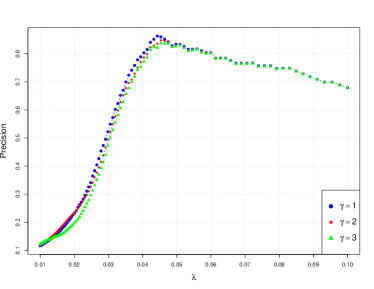
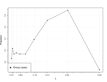
(a) Precision of PISTA under different regularizations.	(b) Precision of group Lasso under different regularizations.
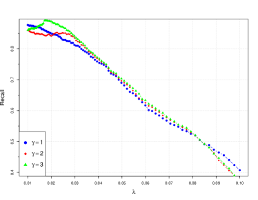
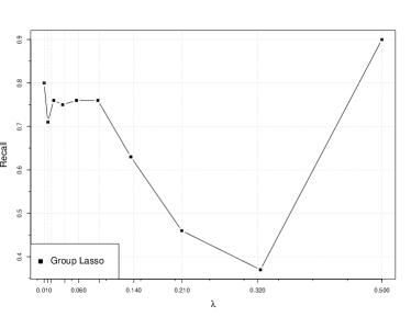
(c) Recall of PISTA under different regularizations.	(d) Recall of group Lasso under different regularizations.
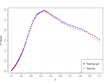
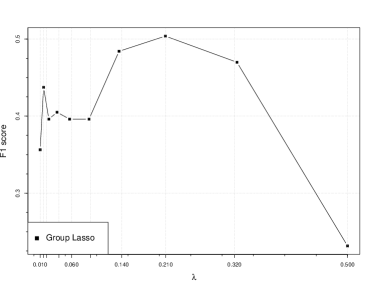
(e) F1 score of PISTA under different regularizations.	(f) F1 score of group Lasso under different regularizations.

Figure 3: PISTA and group Lasso: a side-by-side comparison.

We also list the complete result for the stock market data. This include the complete list of labels and their corresponding companies, as well as the set of causal relationships with sparsity being no more than 3. The results are shown in Tables 2 and LABEL:tab::stock.

Label	Company Name	Label	Company Name
ADBE	Adobe	AMD	Advanced Micro Devices
A	Agilent Technologies	ADI	Analog Devices
AKAM	Akamai Technologies	ALTR	Altair Engineering
AMAT	Applied Materials	ADSK	Autodesk
ADP	Automatic Data Processing	AAPL	Apple
BMC	BMC Software	BRCM	Broadcom
CA	CA Technologies	CTXS	Citrix Systems
CSCO	Cisco Systems	CTSH	Cognizant
CSC	Computer Sciences Corporation	CPWR	Ocean Thermal Energy Corporation
DELL	Dell	EBAY	eBay
ERTS	Electronic Arts	EMC	Dell EMC
FFIV	F5 Networks	FIS	Fidelity National Information Services
FISV	Fiserv Inc	FLIR	FLIR Systems
HRS	Harris Corporation	HPQ	Hewlett Packard Enterprise
INTC	Intel	INTU	Intuit
IBM	International Business Machines	JBL	Jabil Circuit
JDSU	JDS Uniphase Corporation	JNPR	Juniper Networks
KLAC	KLA-Tencor	LSI	LSI Corporation
LXK	Lexmark	LLTC	Linear Technology Corporation
WFR	MEMC Electronic Materials	MCHP	Microchip Technology
MOLX	Molex Inc	MSI	Motorola Solutions
MU	Micron Technology	MSFT	Microsoft Corporation
NSM	National Semiconductor	NTAP	NetApp
NVLS	Novellus Systems	NFLX	Netflix
NVDA	Nvidia	ORCL	Oracle Corporation
PAYX	Paychex Inc	QCOM	Qualcomm
RHT	Red Hat Inc	SNDK	SanDisk
SYMC	Symantec Corporation	TLAB	Tellabs Inc
TER	Teradyne Inc	TXN	Texas Instruments
TSS	Total System Services	VRSN	Verisign Inc
WDC	Western Digital	XRX	Xerox Corporation
XLNX	Xilinx Inc	YHOO	Yahoo Inc

Table 2: Complete set of labels and corresponding company names.

Table 3: Complete set of causal relationships recovered by PISTA and glmnet with sparsity limited to 3. For each row, the companies in the second (or third) column causally affect the company in the first column. For some rows, the number of companies that causal link is strong in the sense that the impact is nonzero even for large values of $\lambda$. For these companies, we keep the causal relations acquired under the largest $\lambda$, which is $0.1$ for PISTA.

Company Label	Causal Relationship (PISTA)	Causal Relationship (glmnet)
ADBE	ALTR, ADSK, FLIR	FLIR, JDSU, KLAC
AMD	KLAC, MU, XRX	ERTS, FLIR, KLAC
A	FLIR, JDSU, NFLX	ERTS, FLIR, JDSU
AKAM	EBAY, NSM, ORCL, SYMC	A, EBAY, KLAC, SNDK
ALTR	DELL, NVLS, SNDK, WDC, XRX	ADBE, BRCM, FLIR, NVDA, WDC
ADI	MU, QCOM, SNDK	FLIR, QCOM, TSS
AAPL	AAPL, DELL, FLIR	AKAM, FLIR, TSS
AMAT	CA, DELL, FLIR	CPWR, FLIR, KLAC
ADSK	JNPR, ORCL, SNDK, TSS	ADSK, ADP, SNDK, TSS
ADP	ADI, INTU, SYMC, WDC	ADP, NFLX, PAYX
BMC	CA, CTSH, FLIR	ADSK, FIS, SNDK
BRCM	ADI, JDSU, LSI	JDSU, LSI, SNDK
CA	CA, DELL, FLIR, MU, MSI	ADSK, FIS, INTU, SNDK, TSS
CSCO	CA, FLIR, JDSU, NVDA	FLIR, JDSU, KLAC, NVDA
CTXS	AKAM, FISV, FLIR	AKAM, FLIR, WDC
CTSH	ADBE, AMD, MOLX, TSS, YHOO	FLIR, PAYX, RHT, WDC, YHOO
CSC	ADP, EMC, QCOM, YHOO	CPWR, QCOM, TSS, YHOO
CPWR	KLAC, SNDK, TSS	KLAC, NVDA, TSS
DELL	ADI, FLIR, INTU, QCOM	ADBE, QCOM, SNDK, TSS
EBAY	ADBE, FFIV, JNPR, MU, YHOO	AMAT, JNPR, KLAC, SYMC
ERTS	MU, TSS, WDC	HRS, TSS, WDC
EMC	CA, CTSH, HPQ	ADSK, KLAC, SNDK
FFIV	BRCM, CA, MU, YHOO	BRCM, MSI, NVDA, YHOO
FIS	ADBE, AAPL, TLAB	HRS, KLAC, RHT
FISV	AKAM, DELL, FLIR, NVLS	AKAM, FLIR, MU, TSS
FLIR	ADBE, ADSK, TSS	JDSU, MU, WDC
HRS	ADSK, CTXS, CSC, EMC	INTU, NVLS, TSS, WDC
HRS	A, ADSK, DELL, FLIR, JBL	INTU, NVLS, TSS, WDC
HPQ	A, ADSK, DELL, FLIR, JBL	FIS, FLIR, INTU, KLAC, TSS
INTC	AKAM, DELL, FFIV,	FLIR, JDSU, MU,
	FLIR, INTU, KLAC	WDC
INTU	FLIR, JBL, NVDA, PAYX	FLIR, JBL, MSI
JBL	FFIV, FLIR, XRX	FLIR, KLAC, WDC
JDSU	DELL, FLIR, PAYX	FLIR, KLAC, TSS
JNPR	ADBE, CTSH, FLIR, MU, NVDA, ORCL	ADBE, KLAC, SNDK, TER
KLAC	ADBE, DELL, FLIR, INTU	FLIR, QCOM, TSS
LXK	ADBE, CA, NVLS, NVDA, SNDK	KLAC, NVDA, TSS
LLTC	AKAM, DELL, INTU,	FLIR, JDSU, SNDK,
	QCOM, SNDK, TLAB	TSS, WDC
LSI	CA, NFLX, TSS	CA, INTU, MSI
WFR	ADBE, CA, RHT	ADBE, KLAC, QCOM
MCHP	ADBE, AKAM, FFIV, JDSU	FLIR, JDSU, QCOM
MU	AKAM, EMC, MU	RHT, SNDK, XRX
MSFT	DELL, NTAP, SNDK	DELL, FLIR, NVDA
MOLX	DELL, FLIR, MU, TSS	FLIR, JDSU, MU, TSS
MSI	AMD, AKAM, ADP,	AKAM, FIS, JDSU,
	BRCM, EMC, INTU	VRSN, YHOO
NSM	JDSU, NVDA, QCOM	FLIR, JDSU, QCOM
NTAP	ADP, JDSU, MU, SNDK	ADP, FLIR, JDSU, SNDK
NFLX	BMC, BRCM, EBAY, EMC, FIS,	FFIV, FLIR, HPQ,
	FLIR, HPQ, MSI, NVLS	ORCL, SNDK, TSS
NVLS	ADBE, FFIV, JDSU	FLIR, JDSU, QCOM
NVDA	ADI, MU, QCOM	LLTC, QCOM, WDC
ORCL	CA, FFIV, FLIR,	AAPL, CA, JDSU,
	JDSU, NVDA, WDC	MSI, SNDK, WDC
PAYX	JBL, JDSU, MCHP, MU	EBAY, JDSU, MU
QCOM	A, FLIR, KLAC, WDC	AAPL, FLIR, TLAB, WDC
RHT	ADSK, DELL, INTC	ADSK, ADP, NVDA
SNDK	ADI, CA, FLIR, MU	BRCM, KLAC, NVDA
SYMC	FFIV, INTU, NFLX	CSC, EMC, WDC
TLAB	CA, FLIR, JDSU, NVDA	FLIR, JDSU, NVDA
TER	BRCM, CTXS, FLIR,	FLIR, JDSU, KLAC,
	JDSU, JNPR, KLAC	NVDA
TXN	CA, DELL, FLIR, QCOM	ADSK, FIS, FLIR, TSS
TSS	CA, FLIR, HPQ,	FLIR, HRS, INTU,
	JBL, JDSU, PAYX, YHOO	JBL, KLAC, TSS
VRSN	LSI, MCHP, MU	AAPL, LSI, TLAB
WDC	LSI, NVDA, VRSN	AMD, NVDA, YHOO
XRX	ADI, TLAB, TSS, XRX	EBAY, TLAB, TSS, XRX
XLXN	DELL, FLIR, MU	FLIR, SNDK, WDC
YHOO	ADBE, FLIR, JDSU, YHOO	ADBE, JDSU, KLAC, TSS

References

• agi (2018) (2018). Agilent company website. https://www.agilent.com/home. [online; accessed 2018-03-10].
• Atanasov and Black (2016) Atanasov, V. and Black, B. (2016). Shock-based causal inference in corporate finance and accounting research .
• Etesami and Kiyavash (2014) Etesami, J. and Kiyavash, N. (2014). Directed information graphs: A generalization of linear dynamical graphs. In American Control Conference (ACC), 2014. IEEE.
• Fan and Li (2001) Fan, J. and Li, R. (2001). Variable selection via nonconcave penalized likelihood and its oracle properties. Journal of the American statistical Association 96 1348–1360.
• Fan and Yao (2008) Fan, J. and Yao, Q. (2008). Nonlinear time series: nonparametric and parametric methods. Springer Science & Business Media.
• Friedman et al. (2001) Friedman, J., Hastie, T. and Tibshirani, R. (2001). The elements of statistical learning, vol. 1. Springer series in statistics New York.
• Friedman et al. (2010) Friedman, J., Hastie, T. and Tibshirani, R. (2010). Regularization paths for generalized linear models via coordinate descent. Journal of statistical software 33 1.
• Granger (1969) Granger, C. W. (1969). Investigating causal relations by econometric models and cross-spectral methods. Econometrica: Journal of the Econometric Society 424–438.
• Han and Liu (2013) Han, F. and Liu, H. (2013). Transition matrix estimation in high dimensional time series. In Proceedings of the 30th International Conference on Machine Learning (ICML-13).
• Hastie and Tibshirani (1990) Hastie, T. and Tibshirani, R. (1990). Generalized additive models. Wiley Online Library.
• Hiemstra and Jones (1994) Hiemstra, C. and Jones, J. D. (1994). Testing for linear and nonlinear granger causality in the stock price-volume relation. The Journal of Finance 49 1639–1664.
• Huang et al. (2012) Huang, J., Breheny, P. and Ma, S. (2012). A selective review of group selection in high-dimensional models. Statistical science: a review journal of the Institute of Mathematical Statistics 27.
• Huang et al. (2010) Huang, J., Horowitz, J. L. and Wei, F. (2010). Variable selection in nonparametric additive models. Annals of Statistics 38 2282–2313.
• Hyvärinen et al. (2008) Hyvärinen, A., Shimizu, S. and Hoyer, P. O. (2008). Causal modelling combining instantaneous and lagged effects: an identifiable model based on non-gaussianity. In Proceedings of the 25th international conference on Machine learning. ACM.
• Jiao et al. (2013) Jiao, J., Permuter, H. H., Zhao, L., Kim, Y.-H. and Weissman, T. (2013). Universal estimation of directed information. Information Theory, IEEE Transactions on 59 6220–6242.
• Kamitake et al. (1984) Kamitake, T., Harashima, H. and Miyakawa, H. (1984). A time-series analysis method based on the directed transinformation. Electronics and Communications in Japan (Part I: Communications) 67 1–9.
• Lin et al. (2006) Lin, Y., Zhang, H. H. et al. (2006). Component selection and smoothing in multivariate nonparametric regression. The Annals of Statistics 34 2272–2297.
• Materassi and Innocenti (2010) Materassi, D. and Innocenti, G. (2010). Topological identification in networks of dynamical systems. Automatic Control, IEEE Transactions on 55 1860–1871.
• Merlevède et al. (2009) Merlevède, F., Peligrad, M., Rio, E. et al. (2009). Bernstein inequality and moderate deviations under strong mixing conditions. In High dimensional probability V: the Luminy volume. Institute of Mathematical Statistics, 273–292.
• Peters et al. (2013) Peters, J., Janzing, D. and Schölkopf, B. (2013). Causal inference on time series using restricted structural equation models. In Advances in Neural Information Processing Systems.
• Quinn et al. (2011) Quinn, C. J., Coleman, T. P., Kiyavash, N. and Hatsopoulos, N. G. (2011). Estimating the directed information to infer causal relationships in ensemble neural spike train recordings. Journal of computational neuroscience 30 17–44.
• Quinn et al. (2015) Quinn, C. J., Kiyavash, N. and Coleman, T. P. (2015). Directed information graphs. Information Theory, IEEE Transactions on 61 6887–6909.
• Ravikumar et al. (2009) Ravikumar, P., Lafferty, J., Liu, H. and Wasserman, L. (2009). Sparse additive models. Journal of the Royal Statistical Society: Series B (Statistical Methodology) 71 1009–1030.
• Rissanen and Wax (1987) Rissanen, J. and Wax, M. (1987). Measures of mutual and causal dependence between two time series (corresp.). IEEE Transactions on information theory 33 598–601.
• Robins et al. (2000) Robins, J. M., Hernan, M. A. and Brumback, B. (2000). Marginal structural models and causal inference in epidemiology.
• Rodriguez et al. (2011) Rodriguez, M. G., Balduzzi, D. and Schölkopf, B. (2011). Uncovering the temporal dynamics of diffusion networks. arXiv preprint arXiv:1105.0697 .
• Rudelson and Vershynin (2013) Rudelson, M. and Vershynin, R. (2013). Hanson-Wright inequality and sub-gaussian concentration. ArXiv e-prints .
• Runge et al. (2015) Runge, J., Petoukhov, V., Donges, J. F., Hlinka, J., Jajcay, N., Vejmelka, M., Hartman, D., Marwan, N., Paluš, M. and Kurths, J. (2015). Identifying causal gateways and mediators in complex spatio-temporal systems. Nature communications 6 8502.
• Runge et al. (2017) Runge, J., Sejdinovic, D. and Flaxman, S. (2017). Detecting causal associations in large nonlinear time series datasets. arXiv preprint arXiv:1702.07007 .
• Stone (1985) Stone, C. J. (1985). Additive regression and other nonparametric models. The annals of Statistics 689–705.
• van Handel (2014) van Handel, R. (2014). Probability in high dimension. Tech. rep., DTIC Document.
• Wang et al. (2014) Wang, Z., Liu, H. and Zhang, T. (2014). Optimal computational and statistical rates of convergence for sparse nonconvex learning problems. Annals of statistics 42 2164.
• Yuan and Lin (2006) Yuan, M. and Lin, Y. (2006). Model selection and estimation in regression with grouped variables. Journal of the Royal Statistical Society: Series B (Statistical Methodology) 68 49–67.
• Zhang (2010) Zhang, C.-H. (2010). Nearly unbiased variable selection under minimax concave penalty. The Annals of statistics 894–942.
• Zhao et al. (2012) Zhao, T., Liu, H., Roeder, K., Lafferty, J. and Wasserman, L. (2012). The huge package for high-dimensional undirected graph estimation in r. Journal of Machine Learning Research 13 1059–1062.
• Zhou and Raskutti (2018) Zhou, H. and Raskutti, G. (2018). Non-parametric sparse additive auto-regressive network models. arXiv preprint arXiv:1801.07644 .
• Zhou et al. (1998) Zhou, S., Shen, X., Wolfe, D. et al. (1998). Local asymptotics for regression splines and confidence regions. The annals of statistics 26 1760–1782.