UT-18-04

March, 2018

Decay Rate of Electroweak Vacuum
in the Standard Model and Beyond

So Chigusa^(a), Takeo Moroi^(a) and Yutaro Shoji^(b)

^(a)Department of Physics, University of Tokyo, Tokyo 113-0033, Japan

^(b)Institute for Cosmic Ray Research, The University of Tokyo, Kashiwa 277-8582, Japan

We perform a precise calculation of the decay rate of the electroweak vacuum in the standard model as well as in models beyond the standard model. We use a recently-developed technique to calculate the decay rate of a false vacuum, which provides a gauge invariant calculation of the decay rate at the one-loop level. We give a prescription to take into account the zero modes in association with translational, dilatational, and gauge symmetries. We calculate the decay rate per unit volume, $\gamma$, by using an analytic formula. The decay rate of the electroweak vacuum in the standard model is estimated to be $\log_{10}\gamma\times{\rm Gyr~{}Gpc^{3}}=-582^{+40~{}+184~{}+144~{}+2}_{-45~{}-329~{}-218~{}-1}$, where the 1st, 2nd, 3rd, and 4th errors are due to the uncertainties of the Higgs mass, the top quark mass, the strong coupling constant and the choice of the renormalization scale, respectively. The analytic formula of the decay rate, as well as its fitting formula given in this paper, is also applicable to models that exhibit a classical scale invariance at a high energy scale. As an example, we consider extra fermions that couple to the standard model Higgs boson, and discuss their effects on the decay rate of the electroweak vacuum.

1 Introduction

In the standard model (SM) of particle physics, it has been known that the Higgs quartic coupling may become negative at a high scale through quantum corrections, so that the Higgs potential develops a deeper vacuum. The detailed shape of the Higgs potential depends on the Higgs and the top masses; with the recently observed Higgs mass of $\sim 125\ {\rm GeV}$, it has been known that the electroweak (EW) vacuum is not absolutely stable if the SM is valid up to $\sim 10^{10}\ {\rm GeV}$ or higher. In such a case, the EW vacuum can decay into the deeper vacuum through tunneling in quantum field theory. The lifetime of the EW vacuum has been one of the important topics in particle physics and cosmology.

The decay rate of the EW vacuum has been discussed for a long time. The calculation of the decay rate at the one-loop level first appeared in [15] and was also discussed in other literature [16, 17, 18, 19, 20, 21, 22, 23, 24, 25]. However, there are subtleties in the treatment of zero modes related to the gauge symmetry breaking, which make it difficult to perform a precise and reliable calculation of the decay rate. The lifetime of a vacuum can be evaluated through a rate of bubble nucleation in unit volume and unit time as formulated in [26, 27]. The rate is expressed in the form of

$$\gamma=\mathcal{A}e^{-\mathcal{B}},$$ (1.1)

where $\mathcal{B}$ is the action of a so-called bounce solution, and prefactor $\mathcal{A}$ is quantum corrections having mass dimension 4. Bounce solution is an $O(4)$ symmetric solution of the Euclidean equations of motion, connecting the two vacua. Although the dominant suppression of the decay rate comes from $\mathcal{B}$, the prefactor $\mathcal{A}$ is also important. This is because of large quantum corrections from the top quarks and the gauge bosons. Thus, it is essential to calculate both $\mathcal{A}$ and $\mathcal{B}$ to determine the decay rate precisely. In the SM, there are infinite bounce solutions owing to (i) the classical scale invariance at a high energy scale, (ii) the global symmetries corresponding to $SU(2)_{L}\times U(1)_{Y}/U(1)_{\rm EM}$, as well as (iii) the translational invariance. For the calculation of the prefactor $\mathcal{A}$, a proper procedure to take account of the effects of the zero modes related to (i) and (ii) were not well understood until recently. In addition, the previous calculations of $\mathcal{A}$ were not performed in a gauge-invariant way, which made the gauge invariance of the result unclear.

Recently, a prescription for the treatments of the gauge zero modes was developed [28, 29], based on which a complete calculation of the decay rate of the EW vacuum became possible. The calculation has been performed by the present authors in a recent publication [25] and also by [24]. The purpose of this paper is to give more complete and detailed discussion about the calculation of the decay rate. In [25], we have numerically evaluated the functional determinants of fluctuation operators, which are necessary for the calculation of the decay rate. Here, we perform the calculation analytically; a part of the analytic results was first given in [24]. The effects of the zero modes and the modes with the lowest angular momentum are carefully taken into account, on which previous works had some confusion. We give fitting formulae of the functional determinants based on analytic results, which are useful for the numerical calculation of the decay rate. We also provide a C++ package to study the ELectroweak VAcuum Stability, ELVAS, which is available at [30].

In this paper, we discuss the calculation of the decay rate of the EW vacuum in detail. We first present a detailed formulation of the calculation of the decay rate at the one-loop level. We derive a complete set of analytic formulae that can be used for any models that exhibit classical scale invariance at a high energy scale like the SM. Then, as one of the important applications, we calculate the decay rate of the EW vacuum in the SM. We find that the lifetime of the EW vacuum is much longer than the age of the universe. There, we see that one-loop corrections from the top quark and the gauge bosons are very large although there is an accidental cancellation. It shows the importance of $\mathcal{A}$ for the evaluation of a decay rate. We also evaluate the decay rates of the EW vacuum for models with extra fermions that couple to the Higgs field. In such models, the EW vacuum tends to be destabilized compared with that of the SM since the quartic coupling of the Higgs field is strongly driven to a negative value. (For discussion about the stability of the EW vacuum in models with extra particles, see [31, 32, 33, 34, 35, 36, 37, 38, 39, 40, 41, 42, 43, 44, 45, 46, 47, 48, 49, 50, 22, 51, 52, 53, 54].) We consider three models that contain, in addition to the SM particles, (i) vector-like fermions having the same SM charges as the left-handed quark and the right-handed down quark, (ii) vector-like fermions with the same SM charges as left-handed lepton and right-handed electron, and (iii) a right-handed neutrino. We give constraints on their couplings and masses, requiring that the lifetime of the EW vacuum be long enough.

This paper is organized as follows. In Section 2, we summarize the formulation for the decay rate at the one-loop level, where we provide an analytic formula for each field that couples to the Higgs boson. The detail of the calculation is given in Appendices A $-$ D. In Section 3, we evaluate the vacuum decay rate in the SM. Readers who are interested only in the results can skip over the former section to this section. In Section 4, we analyze decay rates in models with extra fermions. Finally, we conclude in Section 5.

2 Formulation

We first discuss how we calculate the decay rate of the EW vacuum. In the SM, the EW vacuum becomes unstable due to the renormalization group (RG) running of the quartic coupling constant of the Higgs boson, which makes the quartic coupling constant negative at a high scale. In the SM, the instability occurs when the Higgs amplitude becomes much larger than the EW scale. Since the typical field value for the bounce configuration is around that scale, we can neglect the quadratic term in the Higgs potential.

In this section, we use a toy model with $U(1)$ gauge symmetry to derive relevant formulae. The calculation of the decay rate of the EW vacuum is almost parallel to that in the case with $U(1)$ gauge symmetry; the application to the SM case will be explained in the next section.

2.1 Setup

Let us first summarize the setup of our analysis. We study the decay rate of a false vacuum whose instability is due to an RG running of the quartic coupling constant of a scalar field, $\Phi$. We assume that $\Phi$ is charged under the $U(1)$ gauge symmetry (with charge $+1$); the kinetic term includes

$${\cal L}_{\rm kin}\ni\left[\left(\partial_{\mu}-igA_{\mu}\right)\Phi\right]^{\dagger}\left(\partial_{\mu}-igA_{\mu}\right)\Phi,$$ (2.1)

where $A_{\mu}$ is the gauge field and $g$ is the gauge coupling constant, while we consider the following scalar potential:

$$V(\Phi)=\lambda(\Phi^{\dagger}\Phi)^{2}.$$ (2.2)

The quartic coupling, $\lambda$, depends on the renormalization scale, $\mu$, and is assumed to become negative at a high scale due to the RG effect. As we have mentioned before, we neglect the quadratic term assuming that $\lambda$ becomes negative at a much higher scale. In this setup, the scalar potential has scale invariance at the classical level. In the application to the case of the SM, $\Phi$ corresponds to the Higgs doublet and $\lambda$ corresponds to the Higgs quartic coupling constant.

Hereafter, we perform a detailed study of the effects of the fields coupled to $\Phi$ on the decay rate of the false vacuum. We consider a Lagrangian that contains the following interaction terms:

$$\mathcal{L}_{\rm int}\ni\kappa\sigma^{2}|\Phi|^{2}+(y\Phi\bar{\psi}_{L}\psi_{R}+{\rm h.c.})+V(\Phi),$$ (2.3)

where $\sigma$ is a real scalar field, and $\psi_{L}$ and $\psi_{R}$ are chiral fermions (with relevant $U(1)$ charges). We take $y$ real and $\kappa>0$. We neglect dimensionful parameters that are assumed to be much smaller than the typical scale of the bounce. In addition, gauge fixing is necessary to take into account the effects of gauge boson loops. Following [55, 29], we take the gauge fixing function of the following form:

$$\mathcal{F}=\partial_{\mu}A_{\mu}.$$ (2.4)

Then, the gauge fixing term and the Lagrangian of the ghosts (denoted as $\bar{c}$ and $c$) are given by

$$\mathcal{L}_{\rm GF} =\frac{1}{2\xi}\mathcal{F}^{2},$$ (2.5)

$$\mathcal{L}_{\rm FP} =-\bar{c}\partial_{\mu}\partial_{\mu}c,$$ (2.6)

where $\xi$ is the gauge fixing parameter.

The bounce solution is an $O(4)$ symmetric object [56, 57], and transforms under a global $U(1)$ symmetry. Thus, choosing the center of the bounce at $r=0$ (with $r\equiv\sqrt{x_{\mu}x_{\mu}}$), we can write the bounce solution as

$$\Phi|_{\rm bounce}=\frac{1}{\sqrt{2}}e^{i\theta}\bar{\phi}(r),$$ (2.7)

with our choice of the gauge fixing function, without loss of generality. Here, $\theta$ is a real parameter. The function, $\bar{\phi}$, obeys

$$\partial_{r}^{2}\bar{\phi}(r)+\frac{3}{r}\partial_{r}\bar{\phi}(r)-\lambda\bar{\phi}^{3}(r)=0,$$ (2.8)

with boundary conditions $\partial_{r}\bar{\phi}(0)=0$ and $\bar{\phi}(\infty)=0$. For a negative $\lambda$, we have a series of Fubini-Lipatov instanton solutions [58, 59]:

$$\bar{\phi}(r)=\bar{\phi}_{C}\left(1+\frac{|\lambda|}{8}\bar{\phi}_{C}^{2}r^{2}\right)^{-1},$$ (2.9)

which is parameterized by $\bar{\phi}_{C}$ (i.e., the field value at the center of the bounce). We also define $R$, which gives the size of the bounce, as

$$R\equiv\sqrt{\frac{8}{|\lambda|}}\phi_{C}^{-1}.$$ (2.10)

The action of the bounce is given by

$$\mathcal{B}=\frac{8\pi^{2}}{3|\lambda|}.$$ (2.11)

Notice that the tree level action is independent of $\bar{\phi}_{C}$ owing to the classical scale invariance.

Once the bounce solution is obtained, we may integrate over the fluctuation around it. We expand $\Phi$ as

$$\Phi=\frac{1}{\sqrt{2}}e^{i\theta}\left(\bar{\phi}+h+i\varphi\right),$$ (2.12)

where $h$ and $\varphi$ are the physical Higgs mode and the Nambu-Goldstone (NG) mode, respectively. At the one-loop level, the prefactor can be decomposed as

$$\mathcal{A}e^{-\mathcal{B}}=\frac{\mathcal{A}^{(h)}}{\mathcal{V}_{\rm 4D}}\mathcal{A}^{(\sigma)}\mathcal{A}^{(\psi)}\mathcal{A}^{(A_{\mu},\varphi)}\mathcal{A}^{(c,\bar{c})}e^{-\mathcal{B}},$$ (2.13)

where $\mathcal{V}_{\rm 4D}$ is the volume of spacetime, and $\mathcal{A}^{(X)}$ is the contribution from particle $X$. Each of the factors has a form of

$$\mathcal{A}^{(X)}=\left(\frac{{\rm Det}\mathcal{M}^{(X)}}{{\rm Det}\widehat{\mathcal{M}}^{(X)}}\right)^{w^{(X)}},$$ (2.14)

where $\mathcal{M}^{(X)}$ and $\widehat{\mathcal{M}}^{(X)}$ are the fluctuation operators around the bounce solution and around the false vacuum, respectively. Here, $w^{(X)}=1$ for Dirac fermions and Faddeev-Popov ghosts, and $w^{(X)}=-1/2$ for the other bosonic fields. The fluctuation operator is defined as second derivatives of the action:

$$\mathcal{M}^{(X)}\delta^{(4)}(x-y)=\left\langle\frac{\delta^{2}S(X)}{\delta X(x)\delta X(y)}\right\rangle,$$ (2.15)

where the brackets indicate the evaluation around the bounce solution. In addition, $\widehat{\mathcal{M}}^{(X)}$ can be obtained from $\mathcal{M}^{(X)}$ with replacing $\bar{\phi}$ by the vacuum expectation value at the false vacuum, i.e., $\bar{\phi}\to 0$.

Since the Faddeev-Popov ghosts do not couple to the Higgs boson with the present choice of the gauge fixing function, ${\mathcal{M}}^{(c,\bar{c})}=\widehat{\mathcal{M}}^{(c,\bar{c})}$. Thus, we have

$$\mathcal{A}^{(c,\bar{c})}=1.$$ (2.16)

2.2 Functional determinant

For the evaluation of the functional determinants, we first decompose fluctuations into partial waves, making use of the $O(4)$ symmetry of the bounce [15]. The basis is constructed from $Y_{J,m_{A},m_{B}}(\Omega)$, the hyperspherical function on $S^{3}$ with $\Omega$ being a coordinate on $S^{3}$. The decomposition of each fluctuation is given in Appendix A. Here, $J=0,1/2,1,\cdots$ is a non-negative half-integer that labels the total angular momentum in four dimension, and $m_{A}$ and $m_{B}$ are the azimuthal quantum numbers for the $A$-spin and the $B$-spin of $so(4)\simeq su(2)_{A}\times su(2)_{B}$, respectively. The four-dimensional Laplacian operator acts on the hyperspherical function as

$$-\partial^{2}Y_{J,m_{A},m_{B}}(\Omega)=\frac{L^{2}}{r^{2}}Y_{J,m_{A},m_{B}}(\Omega),$$ (2.17)

with

$$L\equiv\sqrt{4J(J+1)}.$$ (2.18)

In addition, $Y_{J,m_{A},m_{B}}(\Omega)$ is normalized as

$$\int d\Omega|Y_{J,m_{A},m_{B}}|^{2}=1.$$ (2.19)

With the above expansion, the functional determinants can be expressed as

$$\frac{{\rm Det}\mathcal{M}^{(X)}}{{\rm Det}\widehat{\mathcal{M}}^{(X)}}=\prod_{J=0}^{\infty}\left(\frac{{\rm Det}\mathcal{M}^{(X)}_{J}}{{\rm Det}\widehat{\mathcal{M}}^{(X)}_{J}}\right)^{n^{(X)}_{J}},$$ (2.20)

where $\mathcal{M}^{(X)}_{J}$ is the fluctuation operator for each partial wave labeled by $J$. In addition, $n^{(\psi)}_{J}=(2J+1)(2J+2)$ for fermions, and $n^{(X)}_{J}=(2J+1)^{2}$ for the others. The explicit forms of the fluctuation operators are shown in Appendix A. Using a theorem [60, 61, 62, 63, 29], the ratio of the functional determinants can be calculated as

$$\frac{{\rm Det}\mathcal{M}^{(X)}_{J}}{{\rm Det}\widehat{\mathcal{M}}^{(X)}_{J}}=\left(\lim_{r\to\infty}\frac{{\rm Det}\Psi}{{\rm Det}\hat{\Psi}}\right)\left(\lim_{r\to 0}\frac{{\rm Det}\Psi}{{\rm Det}\hat{\Psi}}\right)^{-1},$$ (2.21)

where $\Psi=(\Psi_{1},\Psi_{2},\cdots)$ and $\hat{\Psi}=(\hat{\Psi}_{1},\hat{\Psi}_{2},\cdots)$ are sets of independent solutions of

$$\mathcal{M}^{(X)}_{J}\Psi_{i}= \,0,$$ (2.22)

$$\widehat{\mathcal{M}}^{(X)}_{J}\hat{\Psi}_{i}= \,0,$$ (2.23)

and are regular at $r=0$. Notice that, when $\mathcal{M}^{(X)}_{J}$ is an $n\times n$ object, there are $n$ independent solutions that are regular at $r=0$. Since $\Psi_{i}$ and $\hat{\Psi}_{i}$ obey the same linear differential equation at $r\to\infty$, the ratio of the two determinant converges for each $J$.

With a Fubini-Lipatov instanton, we can calculate the ratio analytically, as first pointed out in [24]. For the convenience of readers, we give the details of the calculation in Appendix A. The ratios are given by

$$\frac{{\rm Det}\mathcal{M}^{(h)}_{J}}{{\rm Det}\widehat{\mathcal{M}}^{(h)}_{J}} =\frac{2J(2J-1)}{(2J+3)(2J+2)},$$ (2.24)

$$\frac{{\rm Det}\mathcal{M}^{(\sigma)}_{J}}{{\rm Det}\widehat{\mathcal{M}}^{(\sigma)}_{J}} =\frac{\Gamma(2J+1)\Gamma(2J+2)}{\Gamma(2J+1-z_{\kappa})\Gamma(2J+2+z_{\kappa})},$$ (2.25)

$$\frac{{\rm Det}\mathcal{M}^{(\psi)}_{J}}{{\rm Det}\widehat{\mathcal{M}}^{(\psi)}_{J}} =\left[\frac{[\Gamma(2J+2)]^{2}}{\Gamma\left(2J+2-z_{y}\right)\Gamma\left(2J+2+z_{y}\right)}\right]^{2},$$ (2.26)

$$\frac{{\rm Det}\mathcal{M}^{(A_{\mu},\varphi)}_{J}}{{\rm Det}\widehat{\mathcal{M}}^{(A_{\mu},\varphi)}_{J}} =\frac{J}{J+1}\left[\frac{\Gamma(2J+1)\Gamma(2J+2)}{\Gamma(2J+1-z_{g})\Gamma(2J+2+z_{g})}\right]^{3}.$$ (2.27)

Here,

$$z_{\kappa}= \,-\frac{1}{2}\left(1-\sqrt{1-8\frac{\kappa}{|\lambda|}}\right),$$ (2.28)

$$~{}z_{g}= \,-\frac{1}{2}\left(1-\sqrt{1-8\frac{g^{2}}{|\lambda|}}\right),$$ (2.29)

$$~{}z_{y}= \,i\frac{y}{\sqrt{\lambda}}.$$ (2.30)

where $g$ is the gauge coupling constant, and $\Gamma(z)$ is the gamma function.

2.3 Zero modes

In the calculation of the decay rate of the EW vacuum with the present setup, there show up zero modes in association with dilatation, translation, and global transformation of the bounce solution. Consequently, $\mathcal{M}_{0}^{(h)},\mathcal{M}_{1/2}^{(h)}$ and $\mathcal{M}_{0}^{(A_{\mu},\varphi)}$ have zero eigenvalues. Their determinants vanish as shown in eqs. (2.24) and (2.27) (see also eq. (A.80)); a naive inclusion of those results gives a divergent behavior of the decay rate, which requires a careful treatment of the zero modes. In the present case, we can consider the effect of each partial wave (labeled by $J$) separately. Thus, in this subsection, we consider the case where the fluctuation operator $\mathcal{M}_{J}^{(X)}$ for a certain value of $J$ has a zero eigenvalue and discuss how to take account of its effect. Because only bosons have zero modes in the calculation of vacuum decay rates, $\mathcal{M}_{J}^{(X)}$ is considered to be a fluctuation operator of a bosonic field.

We first decompose the fluctuation of the bosonic field (denoted as $X$) into eigenstates of the angular momentum:

$$X\ni\sum_{i}c_{i}{\cal G}_{i}(r)Y_{J,m_{A},m_{B}}(\Omega),$$ (2.31)

where $c_{i}$ is the expansion coefficient while ${\cal G}_{i}$ obeys

$$\mathcal{M}_{J}^{(X)}{\cal G}_{i}=\omega_{i}{\cal G}_{i},$$ (2.32)

with $\omega_{i}$ being the eigenvalue. We normalize them as

$$\langle{\cal G}_{i}|{\cal G}_{j}\rangle=\frac{\delta_{ij}}{\mathcal{N}_{i}^{2}},$$ (2.33)

where the inner product is defined by

$$\langle{\cal G}_{i}|{\cal G}_{j}\rangle=\int drr^{3}{\cal G}_{i}^{\dagger}(r){\cal G}_{j}(r).$$ (2.34)

We leave $\mathcal{N}_{i}$’s unspecified since, as we see below, the final result is independent of them. We denote the zero mode as ${\cal G}_{0}$ (and hence $\omega_{0}=0$).

When there is a zero mode, the saddle point approximation for the path integral breaks down and we need to go back to the original path integral. The path integral is defined as the integration over the coefficient $c_{i}$, and the functional determinant of $\mathcal{M}_{J}^{(X)}$ originates from the following integral:

$$\int\prod_{i}\frac{dc_{i}}{\sqrt{2\pi}\mathcal{N}_{i}}e^{-\frac{1}{2}c_{j}c_{k}\langle{\cal G}_{j}|\mathcal{M}_{J}^{(X)}|{\cal G}_{k}\rangle},$$

where the summations over the indices $j$ and $k$ are implicit. Applying the saddle point approximation for the modes other than the zero mode, we get

$$\int\prod_{i}\frac{dc_{i}}{\sqrt{2\pi}\mathcal{N}_{i}}e^{-\frac{1}{2}c_{j}c_{k}\langle{\cal G}_{j}|\mathcal{M}_{J}^{(X)}|{\cal G}_{k}\rangle}=\int\frac{dc_{0}}{\sqrt{2\pi}\mathcal{N}_{0}}\prod_{i\neq 0}\frac{1}{\sqrt{\omega_{i}}}.$$ (2.35)

Notice that $\mathcal{M}^{(X)}_{J}$, ${\cal G}_{i}$ and $\omega_{i}$ may depend on $c_{0}$.

We are interested in the case where there exists a symmetry (at least at the classical level) and the Lagrangian is invariant under a transformation, which we parameterize by $z$. The zero mode is in association with such a symmetry. Then, the transformation of the bounce solution with $z\to z+\delta z$ can be seen as a shift of $X$ as

$$X\to X+\delta z\tilde{{\cal G}}_{0}Y_{J,m_{A},m_{B}}+\mathcal{O}(\delta z^{2}),$$ (2.36)

where the function $\tilde{{\cal G}}_{0}$ is proportional to ${\cal G}_{0}$. The integration over $c_{0}$ can thus be regarded as the integration over the collective coordinate $z$:

$$\frac{dc_{0}}{\sqrt{2\pi}\mathcal{N}_{0}}\rightarrow\sqrt{\frac{\langle\tilde{{\cal G}}_{0}|\tilde{{\cal G}}_{0}\rangle}{2\pi}}dz,$$ (2.37)

and hence

$$\int\prod_{i}\frac{dc_{i}}{\sqrt{2\pi}\mathcal{N}_{i}}e^{-\frac{1}{2}c_{j}c_{k}\langle{\cal G}_{j}|\mathcal{M}_{J}^{(X)}|{\cal G}_{k}\rangle}\to\int dz\sqrt{\frac{\langle\tilde{{\cal G}}_{0}|\tilde{{\cal G}}_{0}\rangle}{2\pi}}\prod_{i\neq 0}\frac{1}{\sqrt{\omega_{i}}}.$$ (2.38)

Next, we discuss how we evaluate the integrand of the right-hand side of eq. (2.38). To omit the zero eigenvalue from the functional determinant, we introduce a regulator to the fluctuation operator:

$$\mathcal{M}_{J}^{(X)}\to\mathcal{M}_{J}^{(X)}+\nu\rho(r),$$ (2.39)

where $\nu$ is a small positive number, and $\rho(r)$ is an arbitrary function that satisfies

$$\langle\tilde{{\cal G}}_{0}|\rho|\tilde{{\cal G}}_{0}\rangle=2\pi.$$ (2.40)

Then, we have

$$\int\prod_{i}\frac{dc_{i}}{\sqrt{2\pi}\mathcal{N}_{i}}e^{-\frac{1}{2}c_{j}c_{k}\langle{\cal G}_{j}|({\mathcal{M}}_{J}^{(X)}+\nu\rho)|{\cal G}_{k}\rangle}=\sqrt{\frac{\langle\tilde{{\cal G}}_{0}|\tilde{{\cal G}}_{0}\rangle}{2\pi}}\frac{1}{\sqrt{\nu+\mathcal{O}(\nu^{2})}}\prod_{i\neq 0}\frac{1}{\sqrt{\omega_{i}+\mathcal{O}(\nu)}},$$ (2.41)

which gives

$$\sqrt{\frac{\langle\tilde{{\cal G}}_{0}|\tilde{{\cal G}}_{0}\rangle}{2\pi}}\prod_{i\neq 0}\frac{1}{\sqrt{\omega_{i}}}=\lim_{\nu\to 0}\sqrt{\nu}\int\prod_{i}\frac{dc_{i}}{\sqrt{2\pi}\mathcal{N}_{i}}e^{-\frac{1}{2}c_{j}c_{k}\langle{\cal G}_{j}|({\mathcal{M}}_{J}^{(X)}+\nu\rho)|{\cal G}_{k}\rangle}.$$ (2.42)

The integration in the above expression is nothing but ${\rm Det}({\mathcal{M}}^{(X)}+\nu\rho)$, and can be evaluated with the use of eq. (2.21). If $\mathcal{M}_{J}^{(X)}$ is a $1\times 1$ object, for example, we obtain

$$\frac{{\rm Det}\left[\mathcal{M}^{(X)}_{J}+\nu\rho\right]}{{\rm Det}\widehat{\mathcal{M}}^{(X)}_{J}}=\nu\lim_{r\to\infty}\frac{\check{\Psi}(r)}{\hat{\Psi}(r)}+\mathcal{O}(\nu^{2}),$$ (2.43)

where

$$\mathcal{M}_{J}^{(X)}\check{\Psi}(r)=-\rho(r)\Psi(r),$$ (2.44)

while the functions $\Psi$ and $\hat{\Psi}$ obey eqs. (2.22) and (2.23), respectively. Then, we interpret the functional determinant of the fluctuation operator with the zero eigenvalue as

$$\left(\frac{{\rm Det}\mathcal{M}^{(X)}_{J}}{{\rm Det}\widehat{\mathcal{M}}^{(X)}_{J}}\right)^{-1/2}\to\int dz\left[\lim_{r\to\infty}\frac{\check{\Psi}(r)}{\hat{\Psi}(r)}\right]^{-1/2}.$$ (2.45)

The above argument can be applied to the zero modes of our interest. In Appendix B, we obtain the following replacements to take care of the dilatational, translational, and gauge zero modes:

$$\left|\frac{{\rm Det}\mathcal{M}^{(h)}_{0}}{{\rm Det}\widehat{\mathcal{M}}^{(h)}_{0}}\right|^{-1/2} \to\int d\ln R\sqrt{\frac{16\pi}{|\lambda|}},$$ (2.46)

$$\left(\frac{{\rm Det}\mathcal{M}^{(h)}_{1/2}}{{\rm Det}\widehat{\mathcal{M}}^{(h)}_{1/2}}\right)^{-2} \to\left(\frac{32\pi}{|\lambda|}\right)^{2}\frac{{\mathcal{V}}_{\rm 4D}}{R^{4}},$$ (2.47)

$$\left(\frac{{\rm Det}\mathcal{M}^{(A_{\mu},\varphi)}_{0}}{{\rm Det}\widehat{\mathcal{M}}^{(A_{\mu},\varphi)}_{0}}\right)^{-1/2} \to\int d\theta\sqrt{\frac{16\pi}{|\lambda|}}.$$ (2.48)

2.4 Renormalization

After taking the product over $J$, we have a UV divergence and thus we need to renormalize the result. In this paper, we use the $\overline{\rm MS}$-scheme, which is based on the dimensional regularization. In this subsection, we explain how the divergences can be subtracted using counter terms in the $\overline{\rm MS}$-scheme.

Since the dimensional regularization cannot be directly used in this evaluation, we first regularize the result by using the angular momentum expansion as

$$\left[\ln\mathcal{A}^{(X)}\right]_{\varepsilon_{X}}\equiv w^{(X)}\sum_{J=0}^{\infty}\frac{n^{(X)}_{J}}{(1+\varepsilon_{X})^{2J}}\ln\left(\frac{{\rm Det}\mathcal{M}^{(X)}_{J}}{{\rm Det}\widehat{\mathcal{M}}^{(X)}_{J}}\right).$$ (2.49)

We call this regularization as “angular momentum regularization.” Here, $\varepsilon_{X}$ is a positive number, which will be taken to be zero at the end of the calculation. Since the divergence is at most a power of $J$, the regularized sum converges. In Appendix C, we calculate the sum analytically, and obtain

$$\left[\ln\mathcal{A}^{(\sigma)}\right]_{\varepsilon_{\sigma}}= \,-\frac{\kappa}{|\lambda|}\left(\frac{1}{\varepsilon_{\sigma}^{2}}+\frac{2}{\varepsilon_{\sigma}}+\frac{\kappa}{3|\lambda|}\ln\varepsilon_{\sigma}\right)-\frac{1}{2}\mathcal{S}_{\sigma}(z_{\kappa})+\mathcal{O}(\varepsilon_{\sigma}),$$ (2.50)

$$\left[\ln\mathcal{A}^{(\psi)}\right]_{\varepsilon_{\psi}}= \,\frac{y^{2}}{|\lambda|}\left(\frac{2}{\varepsilon_{\psi}^{2}}+\frac{5}{\varepsilon_{\psi}}+\frac{1}{3}\frac{y^{2}+2|\lambda|}{|\lambda|}\ln\varepsilon_{\psi}\right)+\mathcal{S}_{\psi}(z_{y})+\mathcal{O}(\varepsilon_{\psi}),$$ (2.51)

where the functions, $\mathcal{S}_{\sigma}$ and $\mathcal{S}_{\psi}$, are given in eqs. (C.13) and (C.16), respectively. In addition, we define

$$\mathcal{A}^{(h)} ={\mathcal{V}}_{\rm 4D}\int d\ln R\frac{1}{R^{4}}\mathcal{A}^{\prime(h)},$$ (2.52)

$$\mathcal{A}^{(A_{\mu},\varphi)} =\int d\theta\mathcal{A}^{\prime(A_{\mu},\varphi)}.$$ (2.53)

Then, the primed quantities are given by

$$\left[\ln\mathcal{A}^{\prime(h)}\right]_{\varepsilon_{h}}= \,-\frac{1}{2}\left[\left(\ln\frac{|\lambda|}{16\pi}\right)+4\left(\ln\frac{|\lambda|}{32\pi}\right)+\sum_{J=1}^{\infty}\frac{(2J+1)^{2}}{(1+\varepsilon_{h})^{2J}}\ln\frac{2J(2J-1)}{(2J+3)(2J+2)}\right]$$

$$= \,3\left(\frac{1}{\varepsilon_{h}^{2}}+\frac{2}{\varepsilon_{h}}-\ln\varepsilon_{h}\right)-\frac{3}{4}-3\gamma_{E}-6\ln A_{G}+\frac{5}{2}\ln\frac{\pi}{3}-\frac{5}{2}\ln\frac{|\lambda|}{8}+\mathcal{O}(\varepsilon_{h}),$$ (2.54)

$$\left[\ln\mathcal{A}^{\prime(A_{\mu},\varphi)}\right]_{\varepsilon_{A}}= \,-\frac{1}{2}\Bigg{[}\left(\ln\frac{|\lambda|}{16\pi}\right)$$

$$\,+\sum_{J=1/2}^{\infty}\frac{(2J+1)^{2}}{(1+\varepsilon_{A})^{2J}}\ln\frac{J}{J+1}\left(\frac{\Gamma(2J+1)\Gamma(2J+2)}{\Gamma(2J+1-z_{g})\Gamma(2J+2+z_{g})}\right)^{3}\Bigg{]}$$

$$= \,-\left(\frac{3g^{2}}{|\lambda|}-1\right)\left(\frac{1}{\varepsilon_{A}^{2}}+\frac{2}{\varepsilon_{A}}\right)-\left(\frac{1}{3}+\frac{g^{4}}{|\lambda|^{2}}\right)\ln\varepsilon_{A}$$

$$\,+\frac{3}{4}-\frac{1}{3}\gamma_{E}-2\ln A_{G}-\frac{1}{2}\ln\frac{|\lambda|}{8\pi}$$

$$\,-\frac{3}{2}\mathcal{S}_{\sigma}(z_{g})-\frac{3}{2}\ln\Gamma(1-z_{g})\Gamma(2+z_{g})+\mathcal{O}(\varepsilon_{A}),$$ (2.55)

where $A_{G}\simeq 1.282$ is the Glaisher number.

Next, we relate the above results with those based on the dimensional regularization in $D$ dimension, which contain the regularization parameter, $\bar{\varepsilon}_{\rm D}$, defined as

$$\frac{1}{\bar{\varepsilon}_{\rm D}}=\frac{2}{4-D}+\ln 4\pi-\gamma_{E},$$ (2.56)

with $\gamma_{E}$ being the Euler’s constant. We convert the results based on two different regularizations by calculating the following quantity:

$$\left[\ln\mathcal{A}^{(X)}\right]_{\rm div} =w^{(X)}{\rm Tr}\left[\left(\widehat{\mathcal{M}}^{(X)}\right)^{-1}\delta\mathcal{M}^{(X)}\right]-\frac{w^{(X)}}{2}{\rm Tr}\left[\left(\widehat{\mathcal{M}}^{(X)}\right)^{-1}\delta\mathcal{M}^{(X)}\left(\widehat{\mathcal{M}}^{(X)}\right)^{-1}\delta\mathcal{M}^{(X)}\right]$$

$$=w^{(X)}\sum_{J=0}^{\infty}n^{(X)}_{J}\left[\ln\frac{{\rm Det}\left[\widehat{\mathcal{M}}^{(X)}_{J}+\delta\mathcal{M}_{J}^{(X)}\right]}{{\rm Det}\widehat{\mathcal{M}}^{(X)}_{J}}\right]_{\mathcal{O}(\delta\mathcal{M}_{J}^{2})},$$ (2.57)

where

$$\delta\mathcal{M}^{(X)}=\mathcal{M}^{(X)}-\widehat{\mathcal{M}}^{(X)},$$ (2.58)

and $\delta\mathcal{M}^{(X)}_{J}$ is defined similarly. Here, $[\cdots]_{\mathcal{O}(\delta)}$ indicates the expansion up to $\delta$. The most important point is that $\left[\ln\frac{{\rm Det}\mathcal{M}^{(X)}}{{\rm Det}\widehat{\mathcal{M}}^{(X)}}\right]_{\rm div}$ has the same divergence as $\left[\ln\frac{{\rm Det}\mathcal{M}^{(X)}}{{\rm Det}\widehat{\mathcal{M}}^{(X)}}\right]$ does when $\delta\mathcal{M}^{(X)}$ does not have a derivative operator.

The first line of eq. (2.57) can be calculated by directly evaluating the traces in a momentum space with using the dimensional regularization; the result is denoted as $\left[\ln\mathcal{A}^{(X)}\right]_{{\rm div},\bar{\varepsilon}_{\rm D}}$. On the other hand, the second line of eq. (2.57) can be evaluated as

$$\left[\ln\frac{{\rm Det}\left[\widehat{\mathcal{M}}^{(X)}_{J}+\delta\mathcal{M}_{J}^{(X)}\right]}{{\rm Det}\widehat{\mathcal{M}}^{(X)}_{J}}\right]_{\mathcal{O}(\delta\mathcal{M}_{J}^{2})}= \,{\rm Tr}\left[\hat{\Psi}^{-1}\Psi^{(1)}\right]+{\rm Tr}\left[\hat{\Psi}^{-1}\Psi^{(2)}\right]$$

$$\,-\frac{1}{2}{\rm Tr}\left[\hat{\Psi}^{-1}\Psi^{(1)}\hat{\Psi}^{-1}\Psi^{(1)}\right],$$ (2.59)

where

$$\widehat{\mathcal{M}}^{(X)}_{J}\Psi^{(p)}=-\delta\mathcal{M}_{J}^{(X)}\Psi^{(p-1)},$$ (2.60)

for $p=1$ and $2$, and $\Psi^{(0)}=\hat{\Psi}$. Then, we calculate

$$\left[\ln\mathcal{A}^{(X)}\right]_{{\rm div},\varepsilon_{X}}\equiv w^{(X)}\sum_{J}\frac{n^{(X)}_{J}}{(1+\varepsilon_{X})^{2J}}\left[\ln\frac{{\rm Det}\left[\widehat{\mathcal{M}}^{(X)}_{J}+\delta\mathcal{M}_{J}^{(X)}\right]}{{\rm Det}\widehat{\mathcal{M}}^{(X)}_{J}}\right]_{\mathcal{O}(\delta\mathcal{M}_{J}^{2})}.$$ (2.61)

We relate the results based on two regularizations by replacing

$$\left[\ln\mathcal{A}^{(X)}\right]_{{\rm div},\varepsilon_{X}}\rightarrow\left[\ln\mathcal{A}^{(X)}\right]_{{\rm div},\bar{\varepsilon}_{\rm D}}.$$ (2.62)

The expressions of $[\ln\mathcal{A}^{(X)}]_{{\rm div},\varepsilon_{X}}$ and $[\ln\mathcal{A}^{(X)}]_{{\rm div},\bar{\varepsilon}_{\rm D}}$ for each field are given in Appendix D, where we further simplify the relation so that the left-hand side only includes terms that are divergent at the limit of $\varepsilon_{X}\to 0$. We summarize the results below:

• Scalar field:

  $$\left(\frac{1}{\varepsilon_{\sigma}^{2}}+\frac{2}{\varepsilon_{\sigma}}+\frac{\kappa}{3|\lambda|}\ln\varepsilon_{\sigma}\right)\rightarrow-1-\frac{\kappa}{3|\lambda|}\left(\frac{1}{2\bar{\varepsilon}_{\rm D}}+1+\gamma_{E}+\ln\frac{\mu R}{2}\right),$$ (2.63)

• Higgs field:

  $$\left(\frac{1}{\varepsilon_{h}^{2}}+\frac{2}{\varepsilon_{h}}-\ln\varepsilon_{h}\right)\rightarrow\frac{1}{2\bar{\varepsilon}_{\rm D}}+\gamma_{E}+\ln\frac{\mu R}{2},$$ (2.64)

• Fermion:

  $$\left(\frac{2}{\varepsilon_{\psi}^{2}}+\frac{5}{\varepsilon_{\psi}}+\frac{1}{3}\frac{y^{2}+2|\lambda|}{|\lambda|}\ln\varepsilon_{\psi}\right)$$

  $$\hskip 12.91663pt\to-\frac{y^{2}}{3|\lambda|}\left(\frac{1}{2\bar{\varepsilon}_{\rm D}}+1+\gamma_{E}+\ln\frac{\mu R}{2}\right)-\frac{2}{3}\left(\frac{1}{2\bar{\varepsilon}_{\rm D}}+\frac{25}{4}+\gamma_{E}+\ln\frac{\mu R}{2}\right),$$ (2.65)

• Gauge and NG fields:

  $$\left(\frac{3g^{2}}{|\lambda|}-1\right)\left(\frac{1}{\varepsilon_{A}^{2}}+\frac{2}{\varepsilon_{A}}\right)+\left(\frac{1}{3}+\frac{g^{4}}{|\lambda|^{2}}\right)\ln\varepsilon_{A}$$

  $$\hskip 12.91663pt\to-\left(\frac{1}{3}+\frac{2g^{2}}{|\lambda|}+\frac{g^{4}}{|\lambda|^{2}}\right)\left(\frac{1}{2\bar{\varepsilon}_{\rm D}}+1+\gamma_{E}+\ln\frac{\mu R}{2}\right)+1+\frac{g^{4}}{|\lambda|^{2}}\left(\frac{31}{3}-\pi^{2}\right)$$ (2.66)

Subtracting $1/\bar{\varepsilon}_{\rm D}$, we obtain the renormalized prefactor in the $\overline{\rm MS}$-scheme.

2.5 Dilatational zero mode

In the calculation of the decay rate of the EW vacuum, we have an integral over $R$ in association with the classical scale invariance, as we saw in eq. (2.46). So far, we have performed a one-loop calculation of the decay rate, based on which the decay rate is found to behave as

$$\gamma^{\rm(one\mathchar 28973\relax loop)}\propto\int d\ln R\frac{1}{R^{4}}\exp\left[-\frac{8\pi^{2}}{3|\lambda(\mu)|}-\frac{8\pi^{2}\beta_{\lambda}^{(1)}}{3|\lambda(\mu)|^{2}}\ln\mu R\right],$$ (2.67)

where $\beta_{\lambda}^{(1)}$ is the one-loop $\beta$-function of $\lambda$. (Here, we only show the $R$- and $\mu$-dependencies of the one-loop corrections.) Thus, using the purely one-loop result, the integral does not converge.

We expect, however, that the integration can converge once higher order effects are properly included. To see the detail of the path integral over the dilatational zero mode, let us denote the decay rate as

$$\gamma^{\rm(full)}=\int d\ln R\frac{e^{-\mathcal{B}_{\rm eff}}}{R^{4}},$$ (2.68)

where $\mathcal{B}_{\rm eff}$ fully takes account of all the effects of higher order loops.

In order to discuss how $\mathcal{B}_{\rm eff}$ should behave, it is instructive to rescale the coordinate variable as

$$\tilde{x}_{\mu}\equiv\sqrt{\frac{|\lambda|}{8}}\bar{\phi}_{C}x_{\mu}=\frac{x_{\mu}}{R},$$ (2.69)

as well as the fields as

$$\tilde{\Phi}\equiv \,\bar{\phi}_{C}^{-1}\Phi,$$ (2.70)

$$\tilde{\sigma}\equiv \,\bar{\phi}_{C}^{-1}\sigma,$$ (2.71)

$$\tilde{A}_{\mu}\equiv \,\bar{\phi}_{C}^{-1}A_{\mu},$$ (2.72)

$$\tilde{c}\equiv \,\bar{\phi}_{C}^{-1}c,$$ (2.73)

$$\tilde{\bar{c}}\equiv \,\bar{\phi}_{C}^{-1}\bar{c},$$ (2.74)

$$\tilde{\psi}\equiv \,\left(\frac{|\lambda|}{8}\right)^{-1/4}\bar{\phi}_{C}^{-3/2}\psi.$$ (2.75)

Using the rescaled fields, all the explicit scales disappear from the action as a result of scale invariance:

$$\frac{1}{\hbar}\int d^{4}x{\cal L}=\frac{1}{\tilde{\hbar}}\int d^{4}\tilde{x}\tilde{\cal L}\left(\frac{\kappa}{|\lambda|},\frac{y}{\sqrt{|\lambda|}},\frac{g}{\sqrt{|\lambda|}}\right),$$ (2.76)

where ${\cal L}$ is the total Lagrangian,

$$\tilde{\hbar}=\frac{|\lambda|}{8}\hbar,$$ (2.77)

and $\tilde{\cal L}$ includes canonically normalized rescaled fields and depends only on the combinations $\frac{\kappa}{|\lambda|}$, $\frac{y}{\sqrt{|\lambda|}}$ and $\frac{g}{\sqrt{|\lambda|}}$. In addition, the rescaled bounce solution is given by

$$\frac{1}{1+\tilde{x}^{2}}.$$ (2.78)

Based on $\tilde{\cal L}$ and $\tilde{\hbar}$, we expect:

• Only positive powers of $\frac{\kappa}{|\lambda|}$, $\frac{y}{\sqrt{|\lambda|}}$ and $\frac{g}{\sqrt{|\lambda|}}$ appear in the decay rate since there is no singularity when any of these goes to zero. In paticular, they cannot be in a logarithmic function.

• When we renormalize divergences using dimensional regularization, we introduce a renormalization scale $\tilde{\mu}$. It is always in a logarithmic function and is related to the original renormalization scale as

  $$\tilde{\mu}=\mu R.$$ (2.79)

• In subtracting zero modes associated with transformations of eq. (2.78), the result should be again a polynomial of $\frac{\kappa}{|\lambda|}$, $\frac{y}{\sqrt{|\lambda|}}$ and $\frac{g}{\sqrt{|\lambda|}}$. Notice that, for each zero mode, we have $\sqrt{1/\tilde{\hbar}}$ since eq. (2.37) implies

  $$\frac{dc_{0}}{\sqrt{2\pi\tilde{\hbar}}\mathcal{N}_{0}}=dz\sqrt{\frac{\langle\tilde{\cal G}_{0}|\tilde{\cal G}_{0}\rangle}{2\pi\tilde{\hbar}}}.$$ (2.80)

• Quantum corrections have $\tilde{\hbar}^{\ell-1}$ at the $\ell$-th loop since the loop expansion is equivalent to the $\tilde{\hbar}$ expansion.

Based on the above arguments, $\mathcal{B}_{\rm eff}$ is expected to be expressed as

$$\mathcal{B}_{\rm eff}=\frac{8\pi^{2}}{3|\lambda(\mu)|}+\frac{n_{\rm zero}}{2}\ln\frac{|\lambda(\mu)|}{8}+\sum_{\ell=1}^{\infty}\left(\frac{|\lambda(\mu)|}{8}\right)^{\ell-1}\mathcal{P}_{\ell}\left(\frac{\kappa(\mu)}{|\lambda(\mu)|},\frac{y(\mu)}{\sqrt{|\lambda(\mu)|}},\frac{g(\mu)}{\sqrt{|\lambda(\mu)|}},\ln\mu R\right),$$ (2.81)

where $\mathcal{P}_{\ell}$ is the contribution at the $\ell$-loop level, and $n_{\rm zero}$ is the number of zero modes.

If the effects of higher order loops are fully taken into account, $\mathcal{B}_{\rm eff}$ should be independent of $\mu$ because the decay rate is a physical quantity; in such a case, we may choose any value of the renormalization scale $\mu$. In the perturbative calculation, the $\mu$-dependence is expected to cancel out order-by-order; as shown in eq. (2.67), we can explicitly see the cancellation of the $\mu$-dependence at the one-loop level [64]. In our calculation so far, however, we only have the one-loop result, in which $\mu$ dependence remains. As indicated in eq. (2.81), the $\mu$ dependence shows up in the form of $\ln^{p}\mu R$ with $p=1$, $2$, $\cdots$. If $|\ln\mu R|\gg 1$, the logarithmic terms from higher order loops may become comparable to the tree-level bounce action and the perturbative calculation breaks down. In order to make our one-loop result reliable, we should take $\mu\sim O(1/R)$, i.e., we use $R$-dependent renormalization scale $\mu$. With such a choice of $\mu$ (as well as with the use of coupling constants evaluated at the renormalization scale $\mu$), the integration over the size of the bounce is dominated only by the region where $|\lambda(1/R)|$ becomes largest. In the case of the SM, the integration over the size of the bounce converges with this prescription as we show in the following section.

2.6 Final result

Here, we summarize the results obtained in the previous subsections and Appendices. The decay rate with a resummation of important logarithmic terms is given by

$$\gamma=\int d\ln R\frac{1}{R^{4}}\left[\mathcal{A}^{\prime(h)}\mathcal{A}^{(\sigma)}\mathcal{A}^{(\psi)}\mathcal{A}^{(A_{\mu},\varphi)}e^{-\mathcal{B}}\right]_{\overline{\rm MS},~{}\mu\sim 1/R},$$ (2.82)

where

$$\left[\ln\mathcal{A}^{\prime(h)}\right]_{\overline{\rm MS}} =-\frac{3}{4}-6\ln A_{G}+\frac{5}{2}\ln\frac{\pi}{3}-\frac{5}{2}\ln\frac{|\lambda|}{8}+3\ln\frac{\mu R}{2},$$ (2.83)

$$\left[\ln\mathcal{A}^{(\sigma)}\right]_{\overline{\rm MS}} =-\frac{1}{2}\mathcal{S}_{\sigma}(z_{\kappa})+\frac{\kappa}{|\lambda|}+\frac{\kappa^{2}}{3|\lambda|^{2}}\left(1+\gamma_{E}+\ln\frac{\mu R}{2}\right),$$ (2.84)

$$\left[\ln\mathcal{A}^{(\psi)}\right]_{\overline{\rm MS}} =-\frac{y^{4}}{3|\lambda|^{2}}\left(1+\gamma_{E}+\ln\frac{\mu R}{2}\right)-\frac{2y^{2}}{3|\lambda|}\left(\frac{25}{4}+\gamma_{E}+\ln\frac{\mu R}{2}\right)+\mathcal{S}_{\psi}(z_{y}),$$ (2.85)

$$\left[\ln\mathcal{A}^{(A_{\mu},\varphi)}\right]_{\overline{\rm MS}} =\ln\mathcal{V}_{G}+\left[\ln\mathcal{A}^{\prime(A_{\mu},\varphi)}\right]_{\overline{\rm MS}},$$ (2.86)

with

$$\left[\ln\mathcal{A}^{\prime(A_{\mu},\varphi)}\right]_{\overline{\rm MS}}= \,\left(\frac{1}{3}+\frac{2g^{2}}{|\lambda|}+\frac{g^{4}}{|\lambda|^{2}}\right)\left(1+\gamma_{E}+\ln\frac{\mu R}{2}\right)$$

$$-\frac{g^{4}}{|\lambda|^{2}}\left(\frac{31}{3}-\pi^{2}\right)-\frac{1}{4}-\frac{1}{3}\gamma_{E}-2\ln A_{G}-\frac{1}{2}\ln\frac{|\lambda|}{8}+\frac{1}{2}\ln\pi$$

$$-\frac{3}{2}\mathcal{S}_{\sigma}(z_{g})-\frac{3}{2}\ln\Gamma(1-z_{g})\Gamma(2+z_{g}).$$ (2.87)

Here, $\mathcal{V}_{G}$ is the volume of the group space generated by the broken generators. The definitions of $\mathcal{S}_{\sigma}(z)$, $\mathcal{S}_{\psi}(z)$ can be found in Appendix C. Here, we note that the analytic results for the scalar, Higgs, and fermion contributions were first given in [24] with different expression. We emphasize that the final result does not depend on the gauge parameter, $\xi$, and hence our result is gauge invariant. The above result is also applicable to the case where the $U(1)$ symmetry is not gauged as explained in Appendix E.

We have also derived fitting formulae of the functions necessary for the calculation of the decay rate; the result is given in Appendix F. The fitting formulae are particularly useful for the numerical calculation of the decay rate. In addition, a C++ package to study the ELectroweak VAcuum Stability, ELVAS, is available at [30], which is also applicable to various models with (approximate) classical scale invariance.

3 Decay Rate of the EW Vacuum in the SM

3.1 Decay rate

Now, we are in a position to discuss the decay rate of the EW vacuum in the SM. As we have discussed, the decay of the EW vacuum is induced by the bounce configuration whose energy scale is much higher than the EW scale. Thus, we approximate the Higgs potential as

$$V(H)=\lambda(H^{\dagger}H)^{2},$$ (3.1)

where $H$ is the Higgs doublet in the SM and $\lambda$ is the Higgs quartic coupling constant. Notice that $\lambda$ depends on the renormalization scale $\mu$; in the SM, $\lambda$ becomes negative when $\mu$ is above $\sim 10^{10}$ GeV with the best-fit values of the SM parameters. In addition, the relevant part of the Yukawa couplings are given by

$$\mathcal{L}_{\rm Yukawa}\ni y_{t}H\bar{q}_{L}t_{R}^{c}+{\rm h.c.},$$ (3.2)

where $q_{L}$ is the left-handed 3rd generation quark doublet, $t_{R}^{c}$ is the right-handed anti-top quark, and $y_{t}$ is the top Yukawa coupling constant.

Assuming that $\lambda<0$, the bounce solution for the SM is given by

$$H|_{\rm bounce}=\frac{1}{\sqrt{2}}e^{i\theta^{a}\sigma^{a}}\begin{pmatrix}0\\ \bar{\phi}(r)\end{pmatrix},$$ (3.3)

where $\sigma^{a}$ is the Pauli matrices and function $\bar{\phi}$ is given by eq. (2.9). In particular, remember that $\bar{\phi}$ contains a free parameter, which we choose $R$, because of the classical scale invariance.

The results given in the previous section can be easily applied to the case of the SM. Taking account of the effects of the (physical) Higgs boson, top quark, and weak bosons (as well as NG bosons), the decay rate of the EW vacuum in the SM can be written in the following form:

$$\gamma=\int d\ln R\frac{1}{R^{4}}\left[\mathcal{A}^{\prime(h)}\mathcal{A}^{(t)}\mathcal{A}^{(W,Z,\varphi)}e^{-\mathcal{B}}\right]_{\overline{\rm MS}}.$$ (3.4)

As we have mentioned, the relevant renormalization scale of the integrand is $\mu\sim O(1/R)$; in the following numerical analysis, we take $\mu=1/R$ unless otherwise stated. If $\lambda(\mu)$ is positive, there is no bounce solution; the integrand is taken to be zero in such a case. In addition, since we neglect the mass term in the Higgs potential, $1/R$ should be much larger than the EW scale. This condition is automatically satisfied in the present analysis because $\lambda$ becomes negative at the scale much higher than the electroweak scale.

The Higgs contribution $A^{\prime(h)}$ is given in eq. (2.83), while the top-quark contributions is given by

$$\left[\ln\mathcal{A}^{(t)}\right]_{\overline{\rm MS}} =\left.3\left[\ln\mathcal{A}^{(\psi)}\right]_{\overline{\rm MS}}\right|_{y\to y_{t}},$$ (3.5)

where the factor of $3$ is the color factor.

As for the gauge contributions, we have $SU(2)_{L}\times U(1)_{Y}/U(1)_{\rm EM}$ broken symmetries, instead of $U(1)$ in our previous example. Thus, we have a different volume of the group space, $\mathcal{V}_{G}$. To calculate $\mathcal{V}_{G}$, we first expand $H$ around the bounce solution with $\theta^{a}=0$ as

$$H=\frac{1}{\sqrt{2}}\begin{pmatrix}i(\varphi^{1}-i\varphi^{2})\\ \bar{\phi}-i\varphi^{3}\end{pmatrix}.$$ (3.6)

Here, $\varphi^{1}$ and $\varphi^{2}$ are NG bosons absorbed by charged $W$-bosons while $\varphi^{3}$ is that by $Z$-boson. With the change of $\theta^{a}$, the NG modes are transformed as

$$\varphi^{a}\to\varphi^{a}+\theta^{a}\tilde{{\cal G}}_{G}Y_{0,0,0}+\mathcal{O}(\theta^{2}),$$ (3.7)

where

$$\tilde{{\cal G}}_{G}=\sqrt{2\pi^{2}}\bar{\phi}.$$ (3.8)

The integration over the zero modes in association with the gauge transformation of the bounce solution can be replaced by the integration over the parameter $\theta^{a}$:

$$\int d^{3}\theta=2\pi^{2}\equiv{\cal V}_{SU(2)},$$ (3.9)

with the above definition of $\theta^{a}$. Then, following the argument given in Appendix B, the gauge contribution is evaluated as

$$\left[\ln\mathcal{A}^{(W,Z,\varphi)}\right]_{\overline{\rm MS}}= \,\ln\mathcal{V}_{SU(2)}+2\left.\left[\ln\mathcal{A}^{\prime(A_{\mu},\varphi)}\right]_{\overline{\rm MS}}\right|_{g\to g_{W}}+\left.\left[\ln\mathcal{A}^{\prime(A_{\mu},\varphi)}\right]_{\overline{\rm MS}}\right|_{g\to g_{Z}},$$ (3.10)

where $\mathcal{A}^{\prime(A_{\mu},\varphi)}$ is given in eq. (2.87), and

$$g_{W}=\frac{g_{2}}{2},~{}g_{Z}=\frac{\sqrt{g_{Y}^{2}+g_{2}^{2}}}{2},$$ (3.11)

with $g_{2}$ and $g_{Y}$ being the gauge coupling constants of $SU(2)_{L}$ and $U(1)_{Y}$, respectively.

3.2 Numerical results

Now, let us evaluate the decay rate of the EW vacuum in the SM. The decay rate of the EW vacuum is very sensitive to the coupling constants in the SM. In our numerical analysis, we use [74]:

$$m_{h} =125.09\pm 0.24,$$ (3.12)

$$m_{t} =173.1\pm 0.6,$$ (3.13)

$$\alpha_{s}(m_{Z}) =0.1181\pm 0.0011,$$ (3.14)

where $m_{h}$ and $m_{t}$ are the Higgs mass and the top mass, respectively, while $\alpha_{s}$ is the strong coupling constant. Following [75], the gauge couplings, the top Yukawa coupling, and the Higgs quartic coupling are determined at $\mu=m_{t}$; the calculations are done in the on-shell scheme at NNLO precision. In addition, we use three-loop QCD and one-loop QED $\beta$-functions [76, 77, 78] together with values in [74] in order to determine the bottom and the tau Yukawa couplings at $\mu=m_{t}$.

First, we show the RG evolution of the SM coupling constants in fig. 1. We use mainly three-loop $\beta$-functions summarized in [75] and the central values for the SM parameters. The black dotted line indicates where $\bar{\phi}_{C}$ reaches the Planck scale $M_{\rm Pl}\simeq 2.4\times 10^{18}\ {\rm GeV}$. We also show the running above the Planck scale, assuming there are no significant corrections from gravity. For $10^{10}\ {\rm GeV}\lesssim\mu\lesssim 10^{30}\ {\rm GeV}$, $\lambda$ becomes negative; for such a region, we use a dashed line to indicate $\lambda<0$.

In order to understand the $\mu$ dependence of $\lambda$, let us show one-loop RG equations of $\lambda$ and $y_{t}$ (although, in our numerical calculation, we use RG equations including two- and three-loop effects and the contribution from the bottom and the tau Yukawa couplings):

$$\left.16\pi^{2}\frac{d\lambda}{d\ln\mu}\right|_{\rm one\mathchar 28973\relax loop} =12\lambda\left(2\lambda+y_{t}^{2}-\frac{g_{Y}^{2}+g_{2}^{2}}{4}-\frac{g_{2}^{2}}{2}\right)-6y_{t}^{4}+6\left(\frac{g_{Y}^{2}+g_{2}^{2}}{4}\right)^{2}+12\left(\frac{g_{2}^{2}}{4}\right)^{2},$$ (3.15)

$$\left.16\pi^{2}\frac{dy_{t}}{d\ln\mu}\right|_{\rm one\mathchar 28973\relax loop} =y_{t}\left(\frac{9}{2}y_{t}^{2}-8g_{3}^{2}-\frac{9}{4}g_{2}^{2}-\frac{17}{12}g_{Y}^{2}\right).$$ (3.16)

At a low energy scale, the term proportional to $y_{t}^{4}$ drives $\lambda$ to a negative value. As the scale increases, $y_{t}$ decreases while $g_{Y}$ increases, which brings $\lambda$ back to a positive value. Notice that $\lambda$ is bounded from below in the SM.

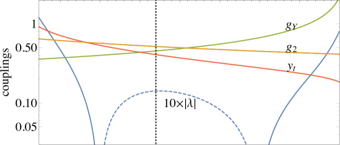
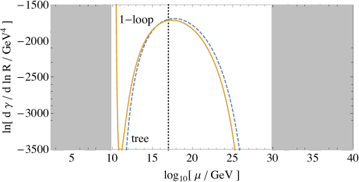
Figure 1: Top: The RG evolution of the SM coupling constants as functions of $\mu$ (in units of GeV). The dashed line indicates $\lambda<0$. The black dotted line shows the scale where $\bar{\phi}_{C}=M_{\rm Pl}$, taking $\mu=1/R$. The horizontal axis is common with the bottom panel. Bottom: The integrand of the decay rate with $\mu=1/R$, taking the central values for the SM parameters. In the shaded region, $\lambda$ is positive and the integrand is zero.

We show the integrand of $\gamma$ in the bottom panel of fig. 1, together with that of

$$\gamma_{\rm tree}=\int d\ln R\frac{1}{R^{4}}e^{-\mathcal{B}}.$$ (3.17)

They are also shown in a linear scale in the top panel of fig. 2.

There are some remarks on the integral over $R$.

• As indicated by the top panel of fig. 2, the integral is dominated by the interval $10^{17}~{}{\rm GeV}\lesssim 1/R<10^{18}~{}{\rm GeV}$, corresponding to $10^{18}~{}{\rm GeV}\lesssim\bar{\phi}_{C}<10^{19}~{}{\rm GeV}$, which is close to the Planck scale. We may formally perform the $R$-integration up to the scale where $\lambda$ becomes positive again; the result of such an analysis is denoted as $\gamma_{\infty}$. Otherwise, we may stop the integration at $\bar{\phi}_{C}\sim M_{\rm Pl}$, expecting that the SM breaks down at the Planck scale due to an effect of quantum gravity; we also perform such a calculation terminating the integral at $\bar{\phi}_{C}=M_{\rm Pl}$, assuming that the bounce solution is unaffected by the effect of quantum gravity. The result is denoted as $\gamma_{\rm Pl}$.

• As one can see in the bottom panel of fig.1, there is an artificial divergence of the integrand at $1/R\simeq 10^{10}\ {\rm GeV}$. This is due to a breakdown of perturbative expansion owing to a too small $|\lambda|$, which makes the one-loop effect larger than the tree-level one. We expect that the effect of such a bounce configuration is unimportant because the bounce action for such a small $|\lambda|$ suppresses the decay rate significantly. Thus, we exclude such a region from the region of integration. In our numerical calculation, we require $\left|\frac{\delta\mathcal{B}_{\rm eff}^{(1)}}{\mathcal{B}}\right|<0.8$ and $\left|\frac{[\ln\mathcal{A}^{(X)}]_{\rm\overline{MS}}}{\mathcal{B}}\right|<0.8$ for each $X$, where $\delta\mathcal{B}_{\rm eff}^{(1)}$ is the one-loop contribution to $\mathcal{B}_{\rm eff}$, and $[\ln\mathcal{A}^{(X)}]_{\rm\overline{MS}}$ is a contribution from particle $X$; the region that does not satisfy these conditions is excluded from the integration.

By numerically integrating over $R$, we obtain

$$\log_{10}\left[\gamma_{\rm Pl}\times{\rm Gyr~{}Gpc^{3}}\right] =-582^{+40~{}+184~{}+144~{}+2}_{-45~{}-329~{}-218~{}-1},$$ (3.18)

$$\log_{10}\left[\gamma_{\infty}\times{\rm Gyr~{}Gpc^{3}}\right] =-580^{+40~{}+183~{}+145~{}+2}_{-44~{}-328~{}-218~{}-1},$$ (3.19)

where the 1st, 2nd, 3rd, and 4th errors are due to the Higgs mass, the top mass, the strong coupling constant, and the renormalization scale, respectively. (In order to estimate the uncertainty due to the choice of the renormalization scale, we vary the renormalization scale from $1/2R$ to $2/R$.) Currently, the largest error comes from the uncertainty of the top mass. With a better understanding of the top quark mass at future LHC experiment [79, 80, 81, 82, 83, 84, 85], or even with at future $e^{+}e^{-}$ colliders [86], more accurate determination of the decay rate will become possible. One can see that the predicted decay rate per unit volume is extremely small, in particular, compared with $H_{0}^{-4}\simeq 10^{3}\ {\rm Gyr~{}Gpc^{3}}$ (with $H_{0}$ being the expansion rate of the present universe). Such a small decay rate is harmless for realizing the present universe observed.

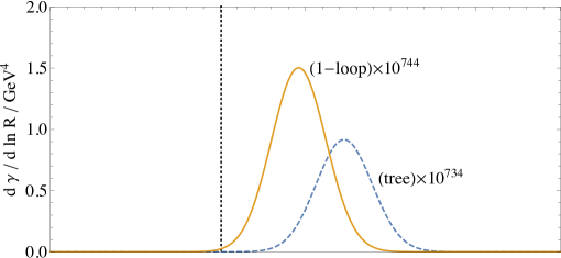
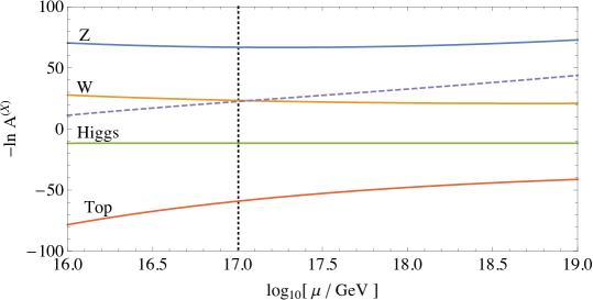
Figure 2: Top: The integrand of the decay rate with the central values of SM parameters. The solid line corresponds to a result at the one-loop level and the dashed one corresponds to that at the tree level. The horizontal axis is common with the bottom figure. We show $\bar{\phi}_{C}=M_{\rm Pl}$ with the vertical dotted line. Bottom: The size of each quantum correction. The dashed line corresponds to $\delta\mathcal{B}^{(1)}_{\rm eff}$.

In fig. 3, we show the decay rate in $m_{h}$ vs. $m_{t}$ plane. In the red region, $\gamma$ becomes larger than $H_{0}^{4}$, which we call unstable region. In the yellow region, the EW vacuum is metastable, meaning that $0<\gamma<H_{0}^{4}$. In the green region, the EW vacuum is absolutely stable because $\lambda$ is always positive. The dashed, solid, and dotted lines correspond to $\alpha_{s}=0.1192,~{}0.1181$, and $0.1170$, respectively. The black dot-dashed contours show $\log_{10}\left[\gamma\times{\rm Gyr~{}Gpc^{3}}\right]=0,-100$, $-300$, and $-1000$ with the central value of $\alpha_{s}$. We also show $68$, $95$, and $99$ % C.L. constraints on the Higgs mass vs. top mass plane assuming that their errors are independently Gaussian distributed. In fig. 3, we terminate the integral at $\bar{\phi}_{C}=M_{\rm Pl}$, but it does not change the figure as far as the cut-off is not so far from the Planck scale. The value of $\bar{\phi}_{C}$ at the maximum of the integrand ranges from $10^{18}$ GeV to $10^{20}$ GeV.

It is well known that, currently, our universe is (almost) dominated by the dark energy. If it is a cosmological constant, then our universe will eventually become de Sitter space with the expansion rate of about $56.3\ {\rm km/sec/Mpc}$ [108]. Then, based on $\gamma_{\rm Pl}$, the phase transition rate within the Hubble volume of such a universe is estimated to be $10^{-580}\ {\rm Gyr}^{-1}$, which may be regarded as a decay rate of the EW vacuum in the SM.

For comparison, we also perform a “tree-level” calculation of the decay rate using eq. (3.17). The results are $\log_{10}\left[\gamma_{\rm Pl}^{\rm(tree)}\times{\rm Gyr~{}Gpc^{3}}\right]=-575$ and $\log_{10}\left[\gamma_{\infty}^{\rm(tree)}\times{\rm Gyr~{}Gpc^{3}}\right]=-570$. Thus, the difference between $\gamma$ and $\gamma^{\rm(tree)}$ turns out to be rather small. This is a consequence of an accidental cancellation among the contributions of several fields. In the bottom panel of fig. 2, we show individual quantum corrections separately, as well as the total one-loop contribution. We can see that the large quantum correction from the top quark is cancelled by those from the gauge bosons. We have also checked that the unstable region on the $m_{h}$ vs. $m_{t}$ plane shifts upward by $\Delta m_{t}\simeq 0.2\ {\rm GeV}$ if we use $\gamma^{\rm(tree)}$.

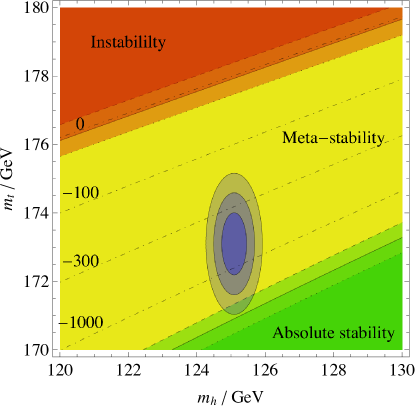
Figure 3: The stability of the EW vacuum in the SM with a cut-off of the integration at $\bar{\phi}_{C}=M_{\rm Pl}$. The red region is unstable, the yellow region is meta-stable, and the green region is absolutely stable. The dashed, solid, and dotted lines correspond to $\alpha_{s}=0.1192$, $0.1181$, and $0.1170$, respectively. The black dot-dashed lines indicate $\log_{10}\left[\gamma\times{\rm Gyr~{}Gpc^{3}}\right]=0$, $-100$, $-300$, and $-1000$ with the central value of $\alpha_{s}$. The blue circles indicate $68$, $95$, and $99$ % C.L. constraints on the Higgs mass vs. top mass plane assuming that their errors are independently Gaussian.

4 Models with Extra Fermions

So far, we assumed that the SM is valid up to the Planck or some higher scale. However, the decay rate of the EW vacuum may be affected if there exist extra particles. In particular, extra fermions coupled to the Higgs boson may destabilize the EW vacuum because the new Yukawa couplings tend to drive $\lambda$ to a negative value through RG effects [32, 33, 34, 35, 36, 37, 38, 39, 40, 41, 42, 43, 46, 48, 49, 50, 51, 52, 54]. Consequently, the decay rate of the EW vacuum becomes larger than that in the SM. Potential candidates of such fermions include vector-like fermions as well as right-handed neutrinos for the seesaw mechanism [109, 110, 111].

In this section, we consider several models with such extra fermions. We perform the RG analysis of the runnings of coupling constants with the effects of the extra fermions. We include two-loop effects of the extra fermions into the $\beta$-functions, which can be calculated using the result in [112, 113, 114, 115]. We also take account of one-loop threshold corrections due to the extra fermions, which are summarized in Appendix G. For the integration over $R$, we follow the procedure in the SM case, as well as the following treatments:

• We terminate the integration if any of the coupling constants (in particular, Yukawa coupling constants of extra particles) exceeds $\sqrt{4\pi}$.

• In order to maintain the classical scale invariance at a good accuracy, we require $1/R>10M_{\rm ex}$, where $M_{\rm ex}$ is the mass scale of the new particles.

4.1 Vector-like fermions

Here, we consider two examples of vector-like fermions, one is colored vector-like fermions and the other is non-colored ones. We consider the case where the extra fermions have a Yukawa coupling with the SM Higgs boson. (We assume that the mixing between the extra fermions and the SM fermions is negligible.)

We first consider colored vector-like fermions, having the same SM gauge quantum numbers as the left-handed quark doublet and the right-handed down quark, as well as their vector-like partners; we add $Q$ $({\bf 3},{\bf 2},\frac{1}{6})$, $\overline{Q}$ $(\bar{\bf 3},{\bf 2},-\frac{1}{6})$, $D$ $({\bf 3},{\bf 1},-\frac{1}{3})$, and $\overline{D}$ $(\bar{\bf 3},{\bf 1},\frac{1}{3})$. (In the parenthesis, we show the quantum numbers of $SU(3)_{C}$, $SU(2)_{L}$, and $U(1)_{Y}$.) The Yukawa terms in the Lagrangian are given by

$$\mathcal{L}_{\rm Yukawa}=\mathcal{L}^{({\rm SM})}_{\rm Yukawa}+Y_{\overline{D}}\Phi^{*}Q\overline{D}+Y_{D}\Phi\overline{Q}D,$$ (4.1)

where $\mathcal{L}_{\rm SM}^{\rm(Yukawa)}$ is the SM part. We also add the following mass terms:

$$\mathcal{L}_{\rm mass}=M_{Q}\overline{Q}Q+M_{D}\overline{D}D.$$ (4.2)

For simplicity, we assume $M_{Q}=M_{D}$. We take the new Yukawa coupling constants and mass parameters real and positive. We also take

$$Y_{D}(\mu=M_{D})=Y_{\overline{D}}(\mu=M_{D})\equiv y_{D}.$$ (4.3)

As we have mentioned before, the scale dependence of the new Yukawa coupling constants is evaluated by using two-loop RG equations and one-loop threshold corrections (see Appendix G).

The calculation of the decay rate is parallel to the SM case, and the decay rate is given in the following form:

$$\gamma=\int d\ln R\frac{1}{R^{4}}\left[\mathcal{A}^{\prime(h)}\mathcal{A}^{(t)}\mathcal{A}^{(A_{\mu},\varphi)}\mathcal{A}^{(Q,\overline{D})}\mathcal{A}^{(\overline{Q},D)}e^{-\mathcal{B}}\right]_{\overline{\rm MS},~{}\mu=1/R},$$ (4.4)

where $\mathcal{A}^{(Q,\overline{D})}$ and $\mathcal{A}^{(\overline{Q},D)}$ are effects of the extra fermions on the prefactor:

$$\left[\ln\mathcal{A}^{(Q,\overline{D})}\right]_{\overline{\rm MS}} =\left.3\left[\ln\mathcal{A}^{(\psi)}\right]_{\overline{\rm MS}}\right|_{y\to Y_{\overline{D}}},$$ (4.5)

$$\left[\ln\mathcal{A}^{(\overline{Q},D)}\right]_{\overline{\rm MS}} =\left.3\left[\ln\mathcal{A}^{(\psi)}\right]_{\overline{\rm MS}}\right|_{y\to Y_{D}}.$$ (4.6)

In fig. 4, we show the contours of the constant decay rate on $M_{D}$ vs. $y_{D}$ plane. Here, we use the central values of the SM parameters. The meanings of the shading colors are the same as in the SM case. The left and the right panels show the results with and without imposing the condition $\bar{\phi}_{C}<M_{\rm Pl}$ in integrating over $R$, respectively. As we can see, the effect of such a cut-off is significant. This is because $\bar{\phi}_{C}$ at the maximum of the integrand, $\bar{\phi}_{C}^{\max}$, can become much larger than the Planck scale in the case with extra fermions; we show $\bar{\phi}_{C}^{\max}$ for the case with vector-like colored fermions in the left panel of fig. 6. (In the upper-left corner of the figure, the value of $\bar{\phi}_{C}^{\max}$ becomes smaller; this is because, in such a region, the Yukawa coupling constants become non-perturbative at a lower RG scale, which gives an upper bound on $\bar{\phi}_{C}$ in the integration over $R$.). To see the cut-off dependence of the decay rate, we show the constraint with terminating the integration at $\bar{\phi}_{C}=0.1M_{\rm Pl}$ in the left panel (dashed line). In addition, when $M_{D}$ and $y_{D}$ are small, we have a region of absolute stability. This is because the addition of colored particles makes the strong coupling constant larger than the SM case. It rapidly drives $y_{t}$ to a small value, which makes $\lambda$ always positive. Requiring that the lifetime of the EW vacuum should be longer than the age of the universe, we obtain $y_{D}\lesssim 0.35-0.5$ for $10^{3}~{}{\rm GeV}\lesssim M_{D}\lesssim 10^{15}~{}{\rm GeV}$.

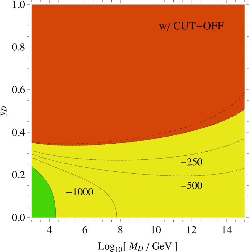
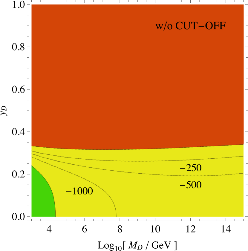
Figure 4: The decay rate of the EW vacuum for vector-like quarks with (left) and without (right) the cut-off at the Planck scale. The red region is unstable, the yellow region is meta-stable, and the green region is absolutely stable. The solid lines show $\log_{10}[\gamma~{}{\rm Gyr}~{}{\rm Gpc}^{3}]=-250,-500$, and $-1000$. The dashed line corresponds to the constraint when we stop the integration at $\bar{\phi}_{C}=0.1M_{\rm Pl}$.

The second example is non-colored extra fermions, having the same SM quantum numbers as leptons. We introduce $L$ $({\bf 1},{\bf 2},-\frac{1}{2})$, $\overline{L}$ $({\bf 1},{\bf 2},\frac{1}{2})$, $E$ $({\bf 1},{\bf 1},-1)$, and $\overline{E}$ $({\bf 1},{\bf 1},1)$, and the Yukawa and mass terms in the Lagrangian are given by

$$\mathcal{L}_{\rm Yukawa} =\mathcal{L}^{({\rm SM})}_{\rm Yukawa}+Y_{\overline{E}}\Phi^{*}L\overline{E}+Y_{E}\Phi\overline{L}E,$$ (4.7)

$$\mathcal{L}_{\rm mass} =M_{L}\overline{L}L+M_{E}\overline{E}E,$$ (4.8)

respectively. For simplicity, we take $M_{L}=M_{E}$ and adopt the following renormalization conditions

$$Y_{E}(\mu=M_{E})=Y_{\overline{E}}(\mu=M_{E})\equiv y_{E}.$$ (4.9)

The decay rate of the EW vacuum is given by

$$\gamma=\int d\ln R\frac{1}{R^{4}}\left[\mathcal{A}^{\prime(h)}\mathcal{A}^{(t)}\mathcal{A}^{(A_{\mu},\varphi)}\mathcal{A}^{(L,\overline{E})}\mathcal{A}^{(\overline{L},E)}e^{-\mathcal{B}}\right]_{\overline{\rm MS},~{}\mu=1/R},$$ (4.10)

where

$$\left[\ln\mathcal{A}^{(L,\overline{E})}\right]_{\overline{\rm MS}} =\left.\left[\ln\mathcal{A}^{(\psi)}\right]_{\overline{\rm MS}}\right|_{y\to Y_{\overline{E}}},$$ (4.11)

$$\left[\ln\mathcal{A}^{(\overline{L},E)}\right]_{\overline{\rm MS}} =\left.\left[\ln\mathcal{A}^{(\psi)}\right]_{\overline{\rm MS}}\right|_{y\to Y_{E}}.$$ (4.12)

In fig. 5, we show the contours of constant decay rate. Since the extra fermions are not colored, we do not have a region of absolute stability. We observe a larger effect of the cut-off at the Planck scale. This is because $\bar{\phi}_{C}^{\max}$ is typically large in a wider parameter space, as indicated in the right panel of fig. 6.

Requiring that the lifetime of the EW vacuum should be longer than the age of the universe, we obtain $y_{E}\lesssim 0.4-0.7$ for $10^{3}~{}{\rm GeV}\lesssim M_{E}\lesssim 10^{15}~{}{\rm GeV}$. The constraint becomes significantly weaker for larger $M_{E}$ owing to the cut-off at the Planck scale.

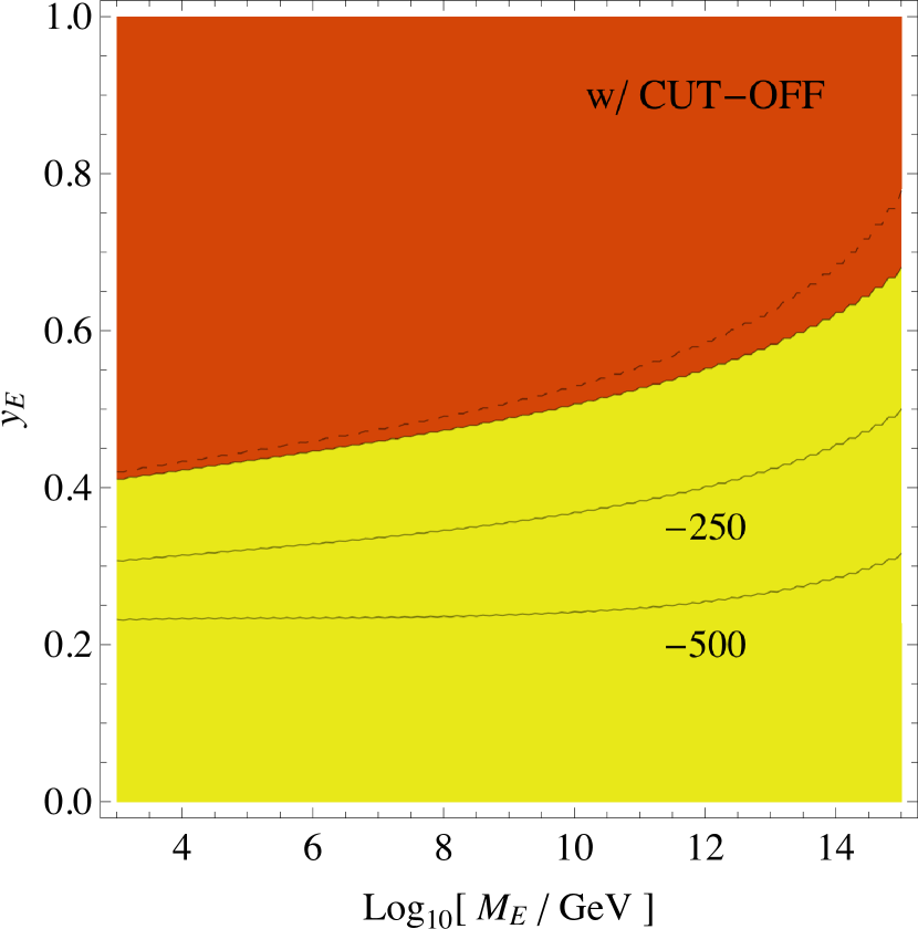
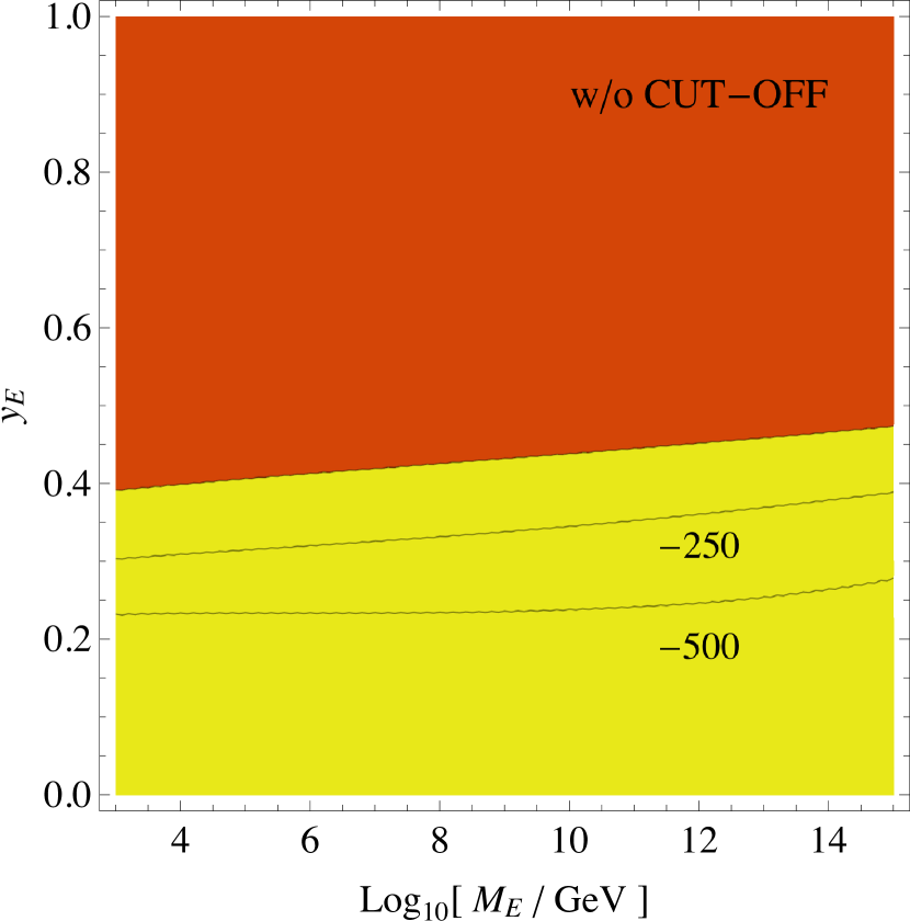
Figure 5: The same figure as fig. 4 but for vector-like leptons.

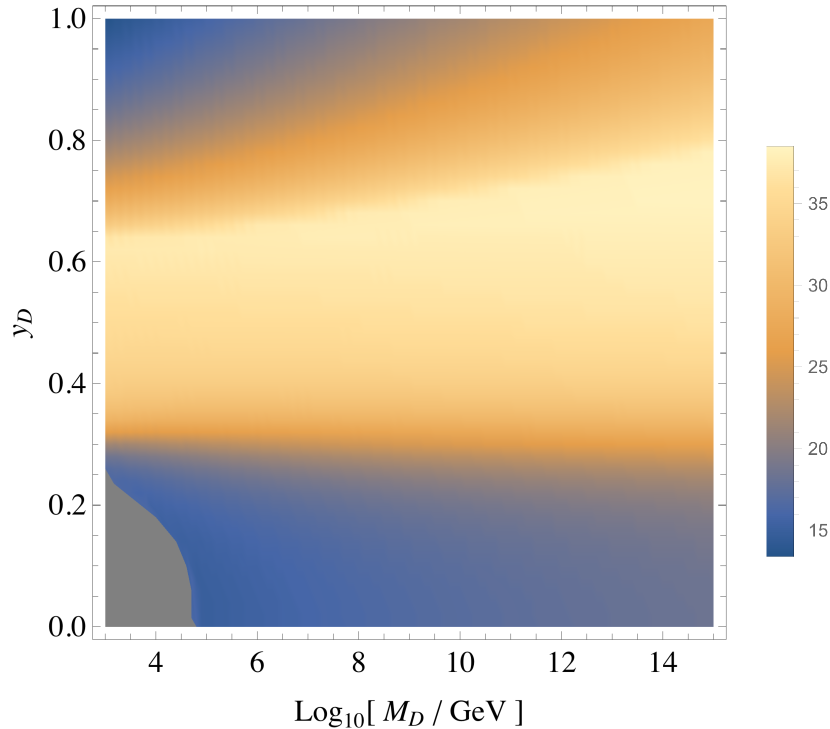
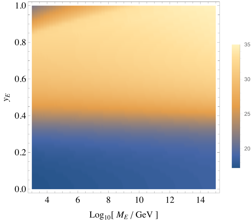
Figure 6: The value of $\bar{\phi}_{C}$ at the maximum of the integrand of $\gamma$, $\bar{\phi}_{C}^{\max}$. The left panel is for vector-like quarks and the right is for vector-like leptons. The numbers in the legends indicate $\log_{10}[\bar{\phi}_{C}^{\max}/{\rm GeV}]$. In the gray region, the EW vacuum is absolutely stable.

4.2 Right-handed neutrino

Next, we consider the case with right-handed neutrinos, which is responsible for the active neutrino masses via the seesaw mechanism [109, 110, 111]. For simplicity, we concentrate on the case where only one mass eigenstate of the right-handed neutrinos, denoted as $N$, strongly couples to the Higgs boson (as well as to the third generation lepton doublet). Then, the Yukawa and mass terms in the Lagrangian are

$$\mathcal{L}_{\rm Yukawa} =\mathcal{L}^{({\rm SM})}_{\rm Yukawa}+Y_{N}\Phi^{*}L\overline{N},$$ (4.13)

$$\mathcal{L}_{\rm mass} =\frac{1}{2}M_{N}\overline{N}N,$$ (4.14)

where, in this subsection, $L$ denotes one of the lepton doublets in the SM. We define

$$Y_{N}(\mu=M_{N})\equiv y_{N}.$$ (4.15)

Assuming that, for simplicity, the neutrino Yukawa matrix is diagonal in the mass-basis of right-handed neutrinos, the following effective operator shows up by integrating out $N$:

$$\Delta\mathcal{L}=\frac{C}{4}(\Phi L)^{2},$$ (4.16)

with

$$C(M_{N})=-2\frac{y_{N}^{2}}{M_{N}}.$$ (4.17)

One of the active neutrino masses is related to the value of $C$ at the EW scale as

$$m_{\nu}=C(m_{t})\frac{v^{2}}{4},$$ (4.18)

with $v\simeq 246\ {\rm GeV}$ being the vacuum expectation value of the Higgs boson. In our numerical calculation, we use the following one-loop RG equation to estimate the neutrino mass [116]:

$$16\pi^{2}\frac{d}{d\ln\mu}C=\left(4\lambda+6y_{t}^{2}-3g_{2}^{2}\right)C.$$ (4.19)

In the SM with right-handed neutrinos, the decay rate of the EW vacuum is evaluated with

$$\gamma=\int d\ln R\frac{1}{R^{4}}\left[\mathcal{A}^{\prime(h)}\mathcal{A}^{(t)}\mathcal{A}^{(A_{\mu},\varphi)}\mathcal{A}^{(L,N)}e^{-\mathcal{B}}\right]_{\overline{\rm MS},~{}\mu=1/R},$$ (4.20)

where

$$\left[\ln\mathcal{A}^{(L,N)}\right]_{\overline{\rm MS}} =\left.\left[\ln\mathcal{A}^{(\psi)}\right]_{\overline{\rm MS}}\right|_{y\to Y_{N}}.$$ (4.21)

In fig. 7, we show the contour plots of the decay rate. Since it does not have any SM charges, the decay rate goes to the SM value when $y_{N}$ goes to zero. The effect of the cut-off at the Planck scale is again large, which is because of a large $\bar{\phi}_{C}^{\max}$ as shown in fig. 8. The purple solid lines show the left-handed neutrino mass. Requiring that the decay rate should be smaller than the age of the universe, we obtain $y_{N}\lesssim 0.65-0.8$ for $10^{12}~{}{\rm GeV}\lesssim M_{N}\lesssim 10^{15}~{}{\rm GeV}$.

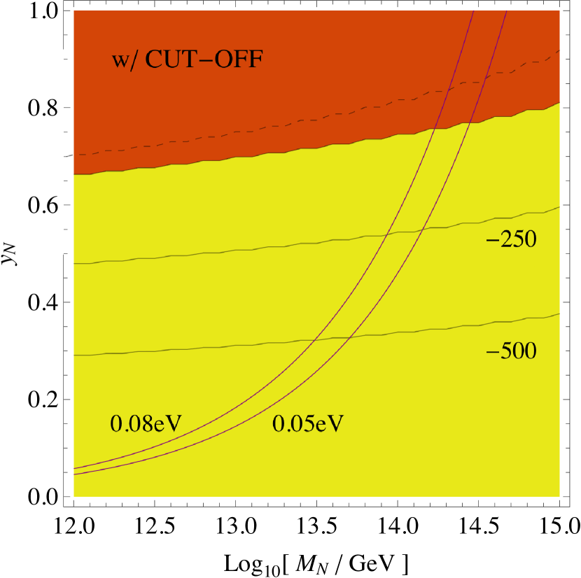
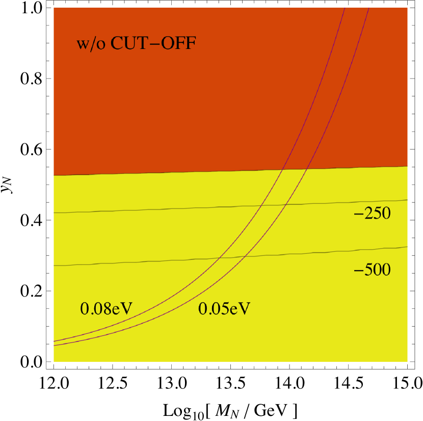
Figure 7: The same figure as fig. 4 but for a right-handed neutrino. We also show lines indicating $m_{\nu}=0.05$ eV and $m_{\nu}=0.08$ eV with purple solid lines.

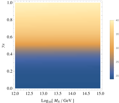
Figure 8: The same figure as fig. 6 but for a right-handed neutrino.

5 Conclusion

In this paper, we have calculated the decay rate of the EW vacuum in the framework of the SM and also in various models with extra fermions. We included the complete one-loop corrections as well as large logarithmic terms in higher loop corrections. We used a recently developed technique to calculate functional determinants in the gauge sector, which not only gives a prescription to perform a gauge invariant calculation of the decay rate but also allows us to calculate the functional determinants analytically. In addition, in calculating the decay rate of the EW vacuum, zero modes show up in association with the dilatational and gauge symmetries. We have properly taken into account their effects, which was not possible in previous calculations. We have given an analytic formula of the decay rate of the EW vacuum, which is also applicable to models that exhibit classical scale invariance at a high energy scale.

The decay rate of the EW vacuum is sensitive to the coupling constants in the SM and their RG behavior. We have used three-loop RG equations for the study of the RG behavior of the SM couplings. The result is used for the precise calculation of the decay rate of the EW vacuum. The decay rate of the EW vacuum is estimated to be

$$\log_{10}\left[\gamma_{\rm Pl}\times{\rm Gyr~{}Gpc^{3}}\right] =-582^{+40~{}+184~{}+144~{}+2}_{-45~{}-329~{}-218~{}-1},$$ (5.1)

where the errors come from the Higgs mass, the top mass, the strong coupling constant, and the renormalization scale, respectively. Here, only the bounce configurations with its amplitude smaller than the Planck scale is taken into account; for the decay rate of the EW vacuum, such a cut-off of the bounce amplitude does not significantly affect the result as far as it is not so far from the Planck scale. Since $H_{0}^{-4}\simeq 10^{3}~{}{\rm Gyr~{}Gpc^{3}}$, the lifetime is long enough compared with the age of the universe.

We have also considered models with extra fermions. Since they typically make the EW vacuum more unstable, the constraints on their masses and couplings are phenomenologically important. We have analyzed the decay rate for the extensions of the SM with (i) vector-like quarks, (ii) vector-like leptons, and (iii) a right-handed neutrino. We have obtained a constraint on the parameter space for each model, requiring that the lifetime be long enough. The results constrain the Yukawa couplings that are larger than about $0.3-0.5$ if we do not consider the cut-off at the Planck scale. The effect of the cut-off was found to be rather large and the constraints on the Yukawa couplings become weaker, at most, by $0.3$ after including the cut-off.

Appendix A Functional Determinant

In this Appendix, we present analytic formulae for various functional determinants. For simplicity, we consider the case with $U(1)$ gauge interaction. The charge of the scalar field that is responsible for the instability, $\Phi$, is set to be $+1$. Application of our results to the case of general gauge groups is straightforward. We are interested in the case where the Lagrangian has (classical) scale invariance; the potential of $\Phi$ is given in eq. (2.2), and the bounce solution is obtained as eq. (2.7).

A.1 Scalar contribution

We first consider a real scalar field, $\sigma$, which couples to $\Phi$ as

$$V=\kappa\sigma^{2}\Phi^{\dagger}\Phi,$$ (A.1)

where $\kappa$ is a positive coupling constant. The contribution to the prefactor is given by

$$\ln\mathcal{A}^{(\sigma)}=-\frac{1}{2}\ln\frac{{\rm Det}[-\partial^{2}+\kappa\bar{\phi}^{2}]}{{\rm Det}[-\partial^{2}]}.$$ (A.2)

First, we expand $\sigma$ into partial waves;

$$\sigma(r,\Omega)=\alpha^{(\sigma)}_{J,m_{A},m_{B}}(r)Y_{J,m_{A},m_{B}}(\Omega).$$ (A.3)

Here and hereafter, $\alpha^{(X)}_{J,m_{A},m_{B}}$ denotes the radial mode function of $X$. For notational simplicity, the summations over $J$, $m_{A}$, and $m_{B}$ are implicit.

Since the fluctuation operator for partial waves does not depend on $m_{A}$ and $m_{B}$, we have $(2J+1)^{2}$ degeneracy for each $J$. Summing up all the contributions,

$$\ln\mathcal{A}^{(\sigma)}=-\frac{1}{2}\sum_{J=0}^{\infty}(2J+1)^{2}\ln\frac{{\rm Det}[-\Delta_{J}+\kappa\bar{\phi}^{2}]}{{\rm Det}[-\Delta_{J}]},$$ (A.4)

where

$$\Delta_{J}=\partial_{r}^{2}+\frac{3}{r}\partial_{r}-\frac{L^{2}}{r^{2}}.$$ (A.5)

Then, using eq. (2.21), we have

$$\frac{{\rm Det}[-\Delta_{J}+\kappa\bar{\phi}^{2}]}{{\rm Det}[-\Delta_{J}]}=\lim_{r\to\infty}\frac{f^{(\sigma)}(r)}{r^{2J}},$$ (A.6)

where the function $f^{(\sigma)}$ satisfies

$$(-\Delta_{J}+\kappa\bar{\phi}^{2})f^{(\sigma)}=0,$$ (A.7)

and $\lim_{r\to 0}f^{(\sigma)}(r)/r^{2J}=1$. The solution of the above differential equation is given by

$$f^{(\sigma)}=r^{2J}\left(1+\frac{|\lambda|}{8}\bar{\phi}_{C}^{2}r^{2}\right)^{1+z_{\kappa}}{}_{2}F_{1}\left(1+z_{\kappa},2(J+1)+z_{\kappa};2(J+1);-\frac{|\lambda|}{8}\bar{\phi}_{C}^{2}r^{2}\right),$$ (A.8)

where ${}_{2}F_{1}(a,b;c;z)$ is the hypergeometric function and

$$z_{\kappa}\equiv-\frac{1}{2}\left(1-\sqrt{1-8\frac{\kappa}{|\lambda|}}\right).$$ (A.9)

Taking the limit of $r\to\infty$, we have

$$\frac{{\rm Det}[-\Delta_{J}+\kappa\bar{\phi}^{2}]}{{\rm Det}[-\Delta_{J}]}=\frac{\Gamma(2J+1)\Gamma(2J+2)}{\Gamma(2J+1-z_{\kappa})\Gamma(2J+2+z_{\kappa})}.$$ (A.10)

A.2 Higgs contribution

Using the bounce solution given in eq. (2.9), the Higgs mode fluctuation is parametrized as

$$\Phi=\frac{1}{\sqrt{2}}\left[\bar{\phi}(r)+\alpha^{(h)}_{J,m_{A},m_{B}}(r)Y_{J,m_{A},m_{B}}(\Omega)\right].$$ (A.11)

Then, the Higgs contribution to the prefactor is given by

$$\ln\mathcal{A}^{(h)} =-\frac{1}{2}\sum_{J=0}^{\infty}(2J+1)^{2}\ln\frac{{\rm Det}[-\Delta_{J}-3|\lambda|\bar{\phi}^{2}]}{{\rm Det}[-\Delta_{J}]}.$$ (A.12)

The functional determinant of the Higgs mode can be obtained with the same procedure as the case of the scalar contribution, taking $\kappa\to-3|\lambda|$:

$$\frac{{\rm Det}[-\Delta_{J}-3|\lambda|\bar{\phi}^{2}]}{{\rm Det}[-\Delta_{J}]}=\frac{2J(2J-1)}{(2J+3)(2J+2)}.$$ (A.13)

As we can see, the above ratio vanishes for $J=0$ and $J=1/2$, which are due to the scale invariance and the translational invariance, respectively.

A.3 Fermion contribution

Let us consider chiral fermions $\psi_{L}$ and $\psi_{R}$ with the following Yukawa term

$$\mathcal{L}^{\rm(Yukawa)}=y\Phi\bar{\psi}_{L}\psi_{R}+{\rm h.c.}$$ (A.14)

The contribution to the prefactor is given by

$$\ln\mathcal{A}^{(\psi)}= \,\ln\frac{{\rm Det}\left[\cancel{\partial}+\frac{y}{\sqrt{2}}\bar{\phi}\right]}{{\rm Det}[\cancel{\partial}]}$$

$$= \,\frac{1}{2}\ln\frac{{\rm Det}\left[\left(\cancel{\partial}+\frac{y}{\sqrt{2}}\bar{\phi}\right)\left(-\cancel{\partial}+\frac{y}{\sqrt{2}}\bar{\phi}\right)\right]}{{\rm Det}[-\cancel{\partial}\cancel{\partial}]}.$$

Taking the basis given in [117], we expand it as

$$\ln\mathcal{A}^{(\psi)} =\sum_{J=0}^{\infty}(2J+1)(2J+2)\ln\frac{{\rm Det}\mathcal{M}^{(\psi)}_{J}}{{\rm Det}\widehat{\mathcal{M}}^{(\psi)}_{J}},$$ (A.16)

where

$$\mathcal{M}^{(\psi)}_{J}=\begin{pmatrix}-\Delta_{J}+\frac{y^{2}}{2}\bar{\phi}^{2}&\frac{y}{\sqrt{2}}\bar{\phi}^{\prime}\\ \frac{y}{\sqrt{2}}\bar{\phi}^{\prime}&-\Delta_{J+1/2}+\frac{y^{2}}{2}\bar{\phi}^{2}\end{pmatrix},$$ (A.17)

with $\bar{\phi}^{\prime}=d\bar{\phi}/dr$, and $\widehat{\mathcal{M}}^{(\psi)}_{J}$ is obtained from $\mathcal{M}^{(\psi)}_{J}$ by replacing $\bar{\phi}\to 0$ and $\bar{\phi}^{\prime}\to 0$.

Using eq. (2.21), we have

$$\frac{{\rm Det}\mathcal{M}^{(\psi)}_{J}}{{\rm Det}\widehat{\mathcal{M}}^{(\psi)}_{J}}=\left(\lim_{r\to\infty}\frac{{\rm Det}[\Psi_{1}~{}\Psi_{2}]}{r^{4J+1}}\right)\left(\lim_{r\to 0}\frac{{\rm Det}[\Psi_{1}~{}\Psi_{2}]}{r^{4J+1}}\right)^{-1},$$ (A.18)

where

$$\mathcal{M}^{(\psi)}_{J}\Psi_{i}(r)=0.$$ (A.19)

Solutions of eq. (A.19) can be expressed by using two functions $\chi^{(\psi)}$ and $\eta^{(\psi)}$ as

$$\Psi_{i}=\begin{pmatrix}\frac{\sqrt{2}}{y\bar{\phi}}\frac{1}{r^{2J+3}}\partial_{r}r^{2J+3}\chi^{(\psi)}_{i}\\ \chi^{(\psi)}_{i}\end{pmatrix}+\begin{pmatrix}-\frac{2}{y^{2}\bar{\phi}^{2}}\frac{1}{r^{2J+3}}\partial_{r}r^{2J+3}\eta^{(\psi)}_{i}\\ 0\end{pmatrix},$$ (A.20)

where $i=1$ and $2$ are for two independent solutions of eq. (A.19), and $\chi^{(\psi)}$ and $\eta^{(\psi)}$ obey

$$\left[-\Delta_{J+1/2}+\frac{\bar{\phi}^{\prime}}{\bar{\phi}}\frac{1}{r^{2J+3}}\partial_{r}r^{2J+3}+\frac{y^{2}}{2}\bar{\phi}^{2}\right]\chi^{(\psi)}_{i} =\frac{\sqrt{2}\bar{\phi}^{\prime}}{y\bar{\phi}^{2}}\frac{1}{r^{2J+3}}\partial_{r}r^{2J+3}\eta^{(\psi)}_{i},$$ (A.21)

$$\left[-\Delta_{J+1/2}+\frac{\bar{\phi}^{\prime}}{\bar{\phi}}\frac{1}{r^{2J+3}}\partial_{r}r^{2J+3}+\frac{y^{2}}{2}\bar{\phi}^{2}\right]\eta^{(\psi)}_{i} =0.$$ (A.22)

For the first solution, we take

$$\chi^{(\psi)}_{1}(r)=f^{(\psi)}(r),~{}\eta^{(\psi)}_{1}(r)=0,$$ (A.23)

where the function $f^{(\psi)}$ satisfies

$$\left[-\Delta_{J+1/2}+\frac{\bar{\phi}^{\prime}}{\bar{\phi}}\frac{1}{r^{2J+3}}\partial_{r}r^{2J+3}+\frac{y^{2}}{2}\bar{\phi}^{2}\right]f^{(\psi)}=0,$$ (A.24)

and

$$\lim_{r\to 0}\frac{f^{(\psi)}(r)}{r^{2J+1}}=1.$$ (A.25)

The analytic formula of $f^{(\psi)}$ is given by

$$f^{(\psi)}(r)=r^{2J+1}\left(1+\frac{|\lambda|}{8}\bar{\phi}_{C}^{2}r^{2}\right)^{-i\frac{y}{\sqrt{|\lambda|}}}{}_{2}F_{1}\left(2J+2-i\frac{y}{\sqrt{|\lambda|}},1-i\frac{y}{\sqrt{|\lambda|}};2J+3;-\frac{|\lambda|}{8}\bar{\phi}_{C}^{2}r^{2}\right),$$ (A.26)

and $f^{(\psi)}$ behaves as

$$\lim_{r\to\infty}\frac{f^{(\psi)}(r)}{r^{2J-1}}=\frac{8}{|\lambda|\bar{\phi}_{C}^{2}}\frac{\Gamma(2J+1)\Gamma(2J+3)}{\Gamma\left(2J+2-i\frac{y}{\sqrt{\lambda}}\right)\Gamma\left(2J+2+i\frac{y}{\sqrt{\lambda}}\right)}.$$ (A.27)

For the second solution, we take

$$\eta^{(\psi)}_{2}(r)=f^{(\psi)}(r).$$ (A.28)

Then, $\chi^{(\psi)}_{2}$ behaves as

$$\lim_{r\to 0}\frac{\chi^{(\psi)}_{2}(r)}{r^{2J+3}} =-\frac{\sqrt{2}\bar{\phi}^{\prime\prime}(0)}{y\bar{\phi}_{C}^{2}}\frac{J+1}{2J+3},$$ (A.29)

$$\lim_{r\to\infty}\frac{\chi^{(\psi)}_{2}(r)}{r^{2J+1}} =\frac{\sqrt{2}}{y\bar{\phi}_{C}}\frac{[\Gamma(2J+2)]^{2}}{\Gamma\left(2J+2-i\frac{y}{\sqrt{\lambda}}\right)\Gamma\left(2J+2+i\frac{y}{\sqrt{\lambda}}\right)}.$$ (A.30)

Using these solutions, we get

$$\lim_{r\to 0}\frac{{\rm Det}[\Psi_{1}~{}\Psi_{2}]}{r^{4J+1}} =\frac{8(J+1)}{y^{2}\bar{\phi}_{C}^{2}},$$ (A.31)

$$\lim_{r\to\infty}\frac{{\rm Det}[\Psi_{1}~{}\Psi_{2}]}{r^{4J+1}} =\frac{8(J+1)}{y^{2}\bar{\phi}^{2}}\left[\frac{[\Gamma(2J+2)]^{2}}{\Gamma\left(2J+2-i\frac{y}{\sqrt{\lambda}}\right)\Gamma\left(2J+2+i\frac{y}{\sqrt{\lambda}}\right)}\right]^{2},$$ (A.32)

and hence

$$\frac{{\rm Det}\mathcal{M}^{(\psi)}_{J}}{{\rm Det}\widehat{\mathcal{M}}^{(\psi)}_{J}}=\left[\frac{[\Gamma(2J+2)]^{2}}{\Gamma\left(2J+2-i\frac{y}{\sqrt{\lambda}}\right)\Gamma\left(2J+2+i\frac{y}{\sqrt{\lambda}}\right)}\right]^{2}.$$ (A.33)

A.4 Gauge contribution

We consider the contributions from gauge bosons, NG bosons, and Faddeev-Popov ghosts. The Lagrangian is given in the following form:

$$\mathcal{L}=\frac{1}{4}F_{\mu\nu}F_{\mu\nu}+\left[\left(\partial_{\mu}-igA_{\mu}\right)\Phi\right]^{\dagger}\left(\partial_{\mu}-igA_{\mu}\right)\Phi+V(\Phi)+\mathcal{L}_{\rm GF}+\mathcal{L}_{\rm FP},$$ (A.34)

where $F_{\mu\nu}$ is the field strength tensor, and

$$\mathcal{L}_{\rm GF} =\frac{1}{2\xi}\mathcal{F}^{2},$$ (A.35)

$$\mathcal{L}_{\rm FP} =\bar{c}(-\partial_{\mu}\partial_{\mu})c,$$ (A.36)

with

$$\mathcal{F}=\partial_{\mu}A_{\mu}.$$ (A.37)

Since Faddeev-Popov ghosts do not directly couple to the Higgs field with our choice of the gauge fixing function, we have

$$\ln\mathcal{A}^{(c,\bar{c})}=0.$$ (A.38)

At the one-loop level, $\ln\mathcal{A}^{(A_{\mu},\varphi)}$ is given by

$$\ln\mathcal{A}^{(A_{\mu},\varphi)} =-\frac{1}{2}\ln\frac{{\rm Det}\mathcal{M}^{(A_{\mu},\varphi)}}{{\rm Det}\widehat{\mathcal{M}}^{(A_{\mu},\varphi)}},$$ (A.39)

where

$$\mathcal{M}^{(A_{\mu},\varphi)}=\begin{pmatrix}-\partial^{2}\delta_{\mu\nu}+\left(1-\frac{1}{\xi}\right)\partial_{\mu}\partial_{\nu}+g^{2}\bar{\phi}^{2}&g(\partial_{\nu}\bar{\phi})-g\bar{\phi}\partial_{\nu}\\ 2g(\partial_{\mu}\bar{\phi})+g\bar{\phi}\partial_{\mu}&-\partial^{2}+V_{\varphi\varphi}\end{pmatrix},$$ (A.40)

with $V_{\varphi\varphi}=d^{2}V/d\varphi^{2}$.

For the partial wave expansions, we use the following basis;

$$A_{\mu}(r,\Omega)= \,\alpha^{(S)}_{J,m_{A},m_{B}}(r)\frac{x_{\mu}}{r}Y_{J,m_{A},m_{B}}(\Omega)+\alpha^{(L)}_{J,m_{A},m_{B}}(r)\frac{r}{L}\partial_{\mu}Y_{J,m_{A},m_{B}}(\Omega)$$

$$\,+\alpha^{(T1)}_{J,m_{A},m_{B}}(r)i\varepsilon_{\mu\nu\rho\sigma}V_{\nu}^{(1)}L_{\rho\sigma}Y_{J,m_{A},m_{B}}(\Omega)$$

$$\,+\alpha^{(T2)}_{J,m_{A},m_{B}}(r)i\varepsilon_{\mu\nu\rho\sigma}V_{\nu}^{(2)}L_{\rho\sigma}Y_{J,m_{A},m_{B}}(\Omega),$$ (A.41)

$$\varphi(r,\Omega)= \,\alpha^{(\varphi)}_{J,m_{A},m_{B}}(r)Y_{J,m_{A},m_{B}}(\Omega),$$ (A.42)

where $V_{\nu}^{(i)}$’s are arbitrary independent vectors and $\varepsilon_{\mu\nu\rho\sigma}$ is a fully anti-symmetric tensor. Then, we have

$$\ln\mathcal{A}^{(A_{\mu},\varphi)} =-\frac{1}{2}\ln\frac{{\rm Det}\mathcal{M}^{(S,\varphi)}_{0}}{{\rm Det}\widehat{\mathcal{M}}^{(S,\varphi)}_{0}}-\frac{1}{2}\sum_{J=1/2}^{\infty}(2J+1)^{2}\left[\ln\frac{{\rm Det}\mathcal{M}^{(S,L,\varphi)}_{J}}{{\rm Det}\widehat{\mathcal{M}}^{(S,L,\varphi)}_{J}}+2\ln\frac{{\rm Det}\mathcal{M}^{(T)}_{J}}{{\rm Det}\widehat{\mathcal{M}}^{(T)}_{J}}\right],$$ (A.43)

where

$$\mathcal{M}^{(S,\varphi)}_{0}= \,\begin{pmatrix}\frac{1}{\xi}\left(-\Delta_{1/2}+\xi g^{2}\bar{\phi}^{2}\right)&g\bar{\phi}^{\prime}-g\bar{\phi}\partial_{r}\\ 2g\bar{\phi}^{\prime}+g\bar{\phi}\frac{1}{r^{3}}\partial_{r}r^{3}&-\Delta_{0}+V_{\varphi\varphi}\end{pmatrix},$$ (A.44)

$$\mathcal{M}^{(S,L,\varphi)}_{J}= \,\begin{pmatrix}-\Delta_{J}+\frac{3}{r^{2}}+g^{2}\bar{\phi}^{2}&-\frac{2L}{r^{2}}&g\bar{\phi}^{\prime}-g\bar{\phi}\partial_{r}\\ -\frac{2L}{r^{2}}&-\Delta_{J}-\frac{1}{r^{2}}+g^{2}\bar{\phi}^{2}&-\frac{L}{r}g\bar{\phi}\\ 2g\bar{\phi}^{\prime}+g\bar{\phi}\frac{1}{r^{3}}\partial_{r}r^{3}&-\frac{L}{r}g\bar{\phi}&-\Delta_{J}+V_{\varphi\varphi}\end{pmatrix}$$

$$\,+\left(1-\frac{1}{\xi}\right)\begin{pmatrix}\Delta_{1/2}&-L\partial_{r}\frac{1}{r}&0\\ \frac{L}{r^{4}}\partial_{r}r^{3}&-\frac{L^{2}}{r^{2}}&0\\ 0&0&0\end{pmatrix},$$ (A.45)

and

$$\mathcal{M}^{(T)}_{J}=-\Delta_{J}+g^{2}\bar{\phi}^{2}.$$ (A.46)

Three independent solutions of $\mathcal{M}^{(S,\varphi)}_{J}\Psi_{i}=0$ (with $i=1-3$) can be constructed from the functions, $\chi_{i}$, $\eta_{i}$, and $\zeta_{i}$, as [28, 29]

$$\Psi_{i}\equiv\begin{pmatrix}\Psi_{i}^{\rm(top)}\\ \Psi_{i}^{\rm(mid)}\\ \Psi_{i}^{\rm(bot)}\end{pmatrix}=\begin{pmatrix}\partial_{r}\chi_{i}\\ \frac{L}{r}\chi_{i}\\ g\bar{\phi}\chi_{i}\end{pmatrix}+\begin{pmatrix}\frac{L}{r}\frac{1}{g^{2}\bar{\phi}^{2}}\eta_{i}\\ \frac{1}{g^{2}\bar{\phi}^{2}}\frac{1}{r^{2}}\partial_{r}r^{2}\eta_{i}\\ 0\end{pmatrix}+\begin{pmatrix}-\frac{2\bar{\phi}^{\prime}}{g^{2}\bar{\phi}^{3}}\zeta_{i}\\ 0\\ \frac{1}{g\bar{\phi}}\zeta_{i}\end{pmatrix},$$ (A.47)

where $\chi_{i}$, $\eta_{i}$, and $\zeta_{i}$ obey

$$\Delta_{J}\chi_{i}=\frac{L}{r}\frac{2\bar{\phi}^{\prime}}{g^{2}\bar{\phi}^{3}}\eta_{i}+\frac{1}{r^{3}}\partial_{r}r^{3}\frac{2\bar{\phi}^{\prime}}{g^{2}\bar{\phi}^{3}}\zeta_{i}-\xi\zeta_{i},$$ (A.48)

$$\left(\Delta_{J}-2\frac{\bar{\phi}^{\prime}}{\bar{\phi}}\frac{1}{r^{2}}\partial_{r}r^{2}-g^{2}\bar{\phi}^{2}\right)\eta_{i}=-2\frac{L}{r}\frac{\bar{\phi}^{\prime}}{\bar{\phi}}\zeta_{i},$$ (A.49)

$$\Delta_{J}\zeta_{i}=0.$$ (A.50)

We also note useful relations:

$$\frac{1}{r^{3}}\partial_{r}r^{3}\Psi^{\rm(top)}_{i} =\frac{L}{r}\Psi_{i}^{\rm(mid)}-\xi\zeta_{i},$$ (A.51)

$$\frac{1}{r}\partial_{r}r\Psi^{\rm(mid)}_{i} =\frac{L}{r}\Psi^{\rm(top)}_{i}+\eta_{i},$$ (A.52)

$$\Psi^{\rm(bot)}_{i} =\frac{rg\bar{\phi}}{L}\Psi^{\rm(mid)}_{i}-\frac{1}{g\bar{\phi}L}\frac{1}{r}\partial_{r}r^{2}\eta_{i}+\frac{1}{g\bar{\phi}}\zeta_{i}.$$ (A.53)

The first solution is obtained by setting $\zeta_{1}=0$ and $\eta_{1}=0$ as

$$\chi_{1}=r^{2J},$$ (A.54)

resulting in

$$\Psi_{1}=\begin{pmatrix}2Jr^{2J-1}\\ Lr^{2J-1}\\ g\bar{\phi}r^{2J}\end{pmatrix}.$$ (A.55)

For the second solution, we set $\zeta_{2}=0$ and

$$\eta_{2}=f^{(\eta)},$$ (A.56)

where the function $f^{(\eta)}$ satisfies

$$\left(\Delta_{J}-2\frac{\bar{\phi}^{\prime}}{\bar{\phi}}\frac{1}{r^{2}}\partial_{r}r^{2}-g^{2}\bar{\phi}^{2}\right)f^{(\eta)}=0,$$ (A.57)

and

$$\lim_{r\to 0}\frac{f^{(\eta)}(r)}{r^{2J}}=1.$$ (A.58)

We can find an analytic formula of $f^{(\eta)}$ as

$$f^{(\eta)}=r^{2J}\left(1+\frac{|\lambda|}{8}\bar{\phi}_{C}^{2}r^{2}\right)^{z_{g}}{}_{2}F_{1}\left(1+z_{g},2(J+1)+z_{g};2(J+1);-\frac{|\lambda|}{8}\bar{\phi}_{C}^{2}r^{2}\right),$$ (A.59)

with

$$z_{g}=-\frac{1}{2}\left(1-\sqrt{1-8\frac{g^{2}}{|\lambda|}}\right).$$ (A.60)

Then, we get

$$\lim_{r\to\infty}\frac{f^{(\eta)}(r)}{r^{2J-2}} =\frac{8}{|\lambda|\bar{\phi}_{C}^{2}}\frac{\Gamma(2J+1)\Gamma(2J+2)}{\Gamma(2J+1-z_{g})\Gamma(2J+2+z_{g})}.$$ (A.61)

Using eqs. (A.51), (A.52), and (A.53), we obtain

$$\lim_{r\to 0}\Psi_{2} =\begin{pmatrix}\frac{Lr^{2J+1}}{8(J+1)}\\ \frac{J+2}{4(J+1)}r^{2J+1}\\ -\frac{2}{g\bar{\phi}_{C}}\frac{J+1}{L}r^{2J}\end{pmatrix},$$ (A.62)

$$\lim_{r\to\infty}\Psi_{2} =\frac{\Gamma(2J+1)\Gamma(2J+2)}{\Gamma(2J+1-z_{g})\Gamma(2J+2+z_{g})}\begin{pmatrix}\frac{4L}{(2J+1)|\lambda|\bar{\phi}^{2}}r^{2J-1}\ln r\\ \frac{8(J+1)}{(2J+1)|\lambda|\bar{\phi}_{C}^{2}}r^{2J-1}\ln r\\ -\frac{2J}{gL\bar{\phi}_{C}}r^{2J}\end{pmatrix}.$$ (A.63)

The last solution can be obtained with

$$\zeta_{3}=r^{2J}.$$ (A.64)

The asymptotic form of $\eta_{3}$ is given by

$$\lim_{r\to 0}\frac{\eta_{3}(r)}{r^{2J+2}}= \,\frac{L|\lambda|\bar{\phi}_{C}^{2}}{16(J+1)},$$ (A.65)

$$\lim_{r\to\infty}\frac{\eta_{3}(r)}{r^{2J}}= \,\frac{L}{2(J+1)}.$$ (A.66)

Using eqs. (A.51), (A.52), and (A.53), we have

$$\lim_{r\to 0}\Psi_{3} =\begin{pmatrix}-\frac{\xi}{4}r^{2J+1}\\ -\frac{J\xi}{2L}r^{2J+1}\\ \frac{1}{g\bar{\phi}_{C}}r^{2J}\end{pmatrix},$$ (A.67)

$$\lim_{r\to\infty}\Psi_{3} =\begin{pmatrix}\frac{J-\xi(J+1)}{4(J+1)}r^{2J+1}\\ \frac{J[(J+2)-\xi(J+1)]}{2L(J+1)}r^{2J+1}\\ \frac{g}{|\lambda|\bar{\phi}_{C}}\frac{(J+2)-\xi(J+1)}{(J+1)^{2}}r^{2J}\end{pmatrix}.$$ (A.68)

We also need three independent solutions around the false vacuum. We take

$$(\hat{\Psi}_{1}~{}\hat{\Psi}_{2}~{}\hat{\Psi}_{3})=\begin{pmatrix}2Jr^{2J-1}&\frac{(J+1)\xi-J}{2L^{2}}r^{2J+1}&0\\ Lr^{2J-1}&\frac{(J+1)\xi-(J+2)}{4L(J+1)}r^{2J+1}&0\\ 0&0&r^{2J}\end{pmatrix}.$$ (A.69)

Then, using eq. (2.21) with combining the above expressions, we obtain the ratio of the functional determinants for $S$, $L$, and NG modes as

$$\frac{{\rm Det}\mathcal{M}^{(S,L,\varphi)}_{J}}{{\rm Det}\widehat{\mathcal{M}}^{(S,L,\varphi)}_{J}}= \,\frac{J}{J+1}\frac{\Gamma(2J+1)\Gamma(2J+2)}{\Gamma(2J+1-z_{g})\Gamma(2J+2+z_{g})}.$$ (A.70)

The functional determinant for $T$ modes can be obtained by using the result for the scalar contribution. With the replacement $\kappa\to g^{2}$ in eq. (A.10):

$$\frac{{\rm Det}\mathcal{M}_{J}^{(T)}}{{\rm Det}\widehat{\mathcal{M}}_{J}^{(T)}}=\frac{\Gamma(2J+1)\Gamma(2J+2)}{\Gamma(2J+1-z_{g})\Gamma(2J+2+z_{g})}.$$ (A.71)

For $J=0$, the solutions of $\mathcal{M}_{0}^{(S,\varphi)}\Psi=0$ can be decomposed as [28, 29]

$$\Psi_{i}\equiv\begin{pmatrix}\Psi_{i}^{\rm(top)}\\ \Psi_{i}^{\rm(bot)}\end{pmatrix}=\begin{pmatrix}\partial_{r}\chi_{i}\\ g\bar{\phi}\chi_{i}\end{pmatrix}+\begin{pmatrix}-\frac{2\bar{\phi}^{\prime}}{g^{2}\bar{\phi}^{3}}\zeta_{i}\\ \frac{1}{g\bar{\phi}}\zeta_{i}\end{pmatrix},$$ (A.72)

with $i=1$ and $2$ for two independent solutions, where the functions $\chi_{i}$ and $\zeta_{i}$ satisfy

$$\Delta_{0}\chi_{i}=\frac{1}{r^{3}}\partial_{r}r^{3}\frac{2\bar{\phi}^{\prime}}{g^{2}\bar{\phi}^{3}}\zeta_{i}-\xi\zeta_{i},$$ (A.73)

$$\Delta_{0}\zeta_{i}=0.$$ (A.74)

Notice that there are useful relations:

$$\frac{1}{r^{3}}\partial_{r}r^{3}\Psi_{i}^{\rm(top)} =-\xi\zeta_{i},$$ (A.75)

$$\partial_{r}\frac{1}{g\bar{\phi}}\Psi_{i}^{\rm(bot)} =\Psi_{i}^{\rm(top)}+\frac{1}{g^{2}\bar{\phi}^{2}}\partial_{r}\zeta_{i}.$$ (A.76)

The first solution is given by

$$\Psi_{1}=\begin{pmatrix}0\\ \frac{\bar{\phi}}{\bar{\phi}_{C}}\end{pmatrix}.$$ (A.77)

The second solution can be obtained with

$$\zeta_{2}=1,$$ (A.78)

giving rise to

$$\Psi_{2}=\begin{pmatrix}-\xi\frac{r}{4}\\ -\xi g\bar{\phi}\frac{r^{2}}{8}\end{pmatrix}.$$ (A.79)

Then, using eq. (2.21), we obrtain

$$\frac{{\rm Det}\mathcal{M}^{(S,\varphi)}_{0}}{{\rm Det}\widehat{\mathcal{M}}^{(S,\varphi)}_{0}}=0.$$ (A.80)

The vanishing of the above ratio is due to the existence of zero mode. The treatment of the zero mode is discussed in Appendix B.

Appendix B Zero Modes

In this Appendix, we discuss the zero modes associated with the dilatation, translation, and global transformation.

B.1 Dilatational zero mode

In $J=0$ mode of the Higgs fluctuation, there exists a dilatational zero mode. The dilatational transformation is parametrized by $\bar{\phi}_{C}$; with $\bar{\phi}_{C}\rightarrow\bar{\phi}_{C}+\delta\bar{\phi}_{C}$, such a change can be absorbed by

$$h\to h+\delta\bar{\phi}_{C}\tilde{{\cal G}}_{D}Y_{0,0,0}+\cdots,$$ (B.1)

where we neglect higher order terms in $\delta\bar{\phi}_{C}$, and

$$\tilde{{\cal G}}_{D}(r)=\sqrt{2\pi^{2}}\frac{d\bar{\phi}}{d\bar{\phi}_{C}}.$$ (B.2)

The second term in the right-hand side of eq. (B.1) is nothing but the change of the amplitude of the dilatational zero mode; one can easily check ${\cal M}^{(h)}_{0}\tilde{{\cal G}}_{D}=0$.

In order to translate the path integral over the dilatational zero mode to the integration over $\bar{\phi}_{C}$, we calculate

$$\frac{{\rm Det}[-\Delta_{0}-3|\lambda|\bar{\phi}^{2}+\nu\rho_{D}(r)]}{{\rm Det}[-\Delta_{0}]},$$ (B.3)

with

$$\rho_{D}(r)=\frac{15}{16\pi}|\lambda|^{2}\bar{\phi}_{C}^{2}\bar{\phi}(r)^{2}.$$ (B.4)

Notice that the condition (2.40) is satisfied with the above choice of $\rho_{D}$, i.e.,

$$\int drr^{3}\tilde{{\cal G}}_{D}^{2}(r)\rho_{D}(r)=2\pi.$$ (B.5)

The ratio of the determinant can be obtained from eq. (A.10) by replacing $\kappa\to-3|\lambda|+\frac{15}{16\pi}|\lambda|^{2}\bar{\phi}_{C}^{2}\nu$. Expanding the result with respect to $\nu$, we get

$$\frac{{\rm Det}[-\Delta_{0}-3|\lambda|\bar{\phi}^{2}+\nu\rho_{D}(r)]}{{\rm Det}[-\Delta_{0}]}=-\nu\frac{|\lambda|}{16\pi}\bar{\phi}_{C}^{2}+\mathcal{O}(\nu^{2}).$$ (B.6)

Thus, we obtain

$$\left|\frac{{\rm Det}[-\Delta_{0}-3|\lambda|\bar{\phi}^{2}]}{{\rm Det}[-\Delta_{0}]}\right|^{-1/2}\to\int d\bar{\phi}_{C}\sqrt{\frac{16\pi}{|\lambda|}}\frac{1}{\bar{\phi}_{C}}=\int d\ln R\sqrt{\frac{16\pi}{|\lambda|}}.$$ (B.7)

Here, we take an absolute value since there is a negative mode [26, 27].

B.2 Translational zero mode

In $J=1/2$ mode of the Higgs fluctuation, translational zero modes exist. The translation is parametrized by the center of the bounce. The shift of the center of the bounce to $a_{\mu}$ can be absorbed by the transformation of the Higgs mode as

$$h\to h+a_{\mu}\tilde{{\cal G}}_{T}Y_{1/2,\mu}+\cdots,$$ (B.8)

where

$$\tilde{{\cal G}}_{T}(r)=-\frac{\pi}{\sqrt{2}}\frac{d\bar{\phi}}{dr},$$ (B.9)

and

$$Y_{1/2,\mu}(\hat{x})=\frac{\sqrt{2}}{\pi}\hat{x}_{\mu},$$ (B.10)

with $\hat{x}_{\mu}=x_{\mu}/|x|$. Notice that $Y_{1/2,\mu}$ is given by a linear combination of $Y_{1/2,m_{A},m_{B}}$ with the same normalization as $Y_{1/2,m_{A},m_{B}}$. Thus, as noted in [27], the path integral over the translational zero modes can be converted to the integration over the spacetime volume.

In order to take care of the translational zero mode, we calculate

$$\frac{{\rm Det}[-\Delta_{1/2}-3|\lambda|\bar{\phi}^{2}+\rho_{T}(r)\nu]}{{\rm Det}[-\Delta_{1/2}]},$$ (B.11)

with

$$\rho_{T}(r)=\frac{3|\lambda|}{4\pi}.$$ (B.12)

One can see that

$$\int drr^{3}\tilde{{\cal G}}_{T}^{2}(r)\rho_{T}(r)=2\pi,$$ (B.13)

which is consistent with eq. (2.40).

Following the argument in Subsection 2.3, we have

$$\left(\frac{{\rm Det}[-\Delta_{1/2}-3|\lambda|\bar{\phi}^{2}]}{{\rm Det}[-\Delta_{1/2}]}\right)^{-2}\to\int d^{4}a\lim_{r\rightarrow\infty}\left(\frac{\check{f}^{(h)}_{1/2}}{r}\right)^{-2},$$ (B.14)

where

$$[-\Delta_{1/2}-3|\lambda|\bar{\phi}^{2}]\check{f}^{(h)}_{1/2}=-\rho_{T}f_{1/2}^{(h)},$$ (B.15)

with

$$f_{1/2}^{(h)}=-\frac{4}{|\lambda|\bar{\phi}_{C}^{3}}\frac{d\bar{\phi}}{dr}.$$ (B.16)

The function $\check{f}^{(h)}_{1/2}$ behaves as

$$\lim_{r\to\infty}\frac{\check{f}^{(h)}_{1/2}}{r}=\frac{1}{4\pi\bar{\phi}_{C}^{2}}.$$ (B.17)

Thus, we obtain

$$\left(\frac{{\rm Det}[-\Delta_{1/2}-3|\lambda|\bar{\phi}^{2}]}{{\rm Det}[-\Delta_{1/2}]}\right)^{-2}\to\left(\frac{32\pi}{|\lambda|}\right)^{2}\left(\frac{|\lambda|}{8}\bar{\phi}_{C}^{2}\right)^{2}\mathcal{V}_{\rm 4D}=\left(\frac{32\pi}{|\lambda|}\right)^{2}\frac{\mathcal{V}_{\rm 4D}}{R^{4}},$$ (B.18)

where $\mathcal{V}_{\rm 4D}$ is the spacetime volume.

B.3 Gauge zero mode

In $J=0$ mode of the gauge field, we have a gauge zero mode. For the case of the $U(1)$ gauge symmetry, the bounce solution is parameterized as eq. (2.7) with the parameter $\theta$. The path integral over the gauge zero mode can be understood as the integration over the variable $\theta$, as we see below.

The effect of the shift $\theta\rightarrow\theta+\delta\theta$ can be absorbed by the transformation of the NG mode as

$$\varphi\to\varphi+\delta\theta\tilde{{\cal G}}_{G}Y_{0,0,0}+\cdots,$$ (B.19)

where

$$\tilde{{\cal G}}_{G}=\sqrt{2\pi^{2}}\bar{\phi}.$$ (B.20)

Using the equation of motion of the bounce solution, the following relation holds:

$$\mathcal{M}^{(S,\varphi)}_{0}\begin{pmatrix}0\\ \tilde{\cal G}_{G}\end{pmatrix}=0.$$ (B.21)

In order to deal with gauge zero mode, we calculate

$$\frac{{\rm Det}\left[\mathcal{M}_{0}^{(S,\varphi)}+\nu\rho_{G}(r)\right]}{{\rm Det}\widehat{\mathcal{M}}_{0}^{(S,\varphi)}},$$ (B.22)

with

$$\rho_{G}(r)=\frac{|\lambda|^{2}}{16\pi}\bar{\phi}_{C}\bar{\phi}.$$ (B.23)

Notice that the following relation holds:

$$\int drr^{3}\tilde{{\cal G}}_{G}^{2}(r)\rho_{G}(r)=2\pi.$$ (B.24)

For the evaluaton of the ratio (B.22) at the leading order in $\nu$, we introduce the function $\check{\Psi}_{1}$ satisfying

$$\mathcal{M}^{(S,\varphi)}_{0}\check{\Psi}_{1}(r)=-\rho_{G}(r)\Psi_{1}(r).$$ (B.25)

with which

$$\left(\frac{{\rm Det}\mathcal{M}^{(S,\varphi)}_{0}}{{\rm Det}\widehat{\mathcal{M}}^{(S,\varphi)}_{0}}\right)^{-1/2}\to\int d\theta\left(\lim_{r\to\infty}\frac{{\rm Det}[\check{\Psi}_{1}(r)~{}\Psi_{2}(r)]}{r}\right)^{-1/2}\left(\lim_{r\to 0}\frac{{\rm Det}[\Psi_{1}(r)~{}\Psi_{2}(r)]}{r}\right)^{1/2}.$$ (B.26)

We can decompose $\check{\Psi}_{1}$ as

$$\check{\Psi}_{1}=\begin{pmatrix}\partial_{r}\check{\chi}_{1}\\ g\bar{\phi}\check{\chi}_{1}\end{pmatrix}+\begin{pmatrix}-\frac{2\bar{\phi}^{\prime}}{g^{2}\bar{\phi}^{3}}\check{\zeta}_{1}\\ \frac{1}{g\bar{\phi}}\check{\zeta}_{1}\end{pmatrix},$$ (B.27)

where $\check{\chi}_{1}$ and $\check{\zeta}_{1}$ satisfies

$$\Delta_{0}\check{\chi}_{1}=\frac{1}{r^{3}}\partial_{r}r^{3}\frac{2\bar{\phi}^{\prime}}{g^{2}\bar{\phi}^{3}}\check{\zeta}_{1}-\xi\check{\zeta}_{1},$$ (B.28)

$$\Delta_{0}\check{\zeta}_{1}=g\rho_{G}\frac{\bar{\phi}^{2}}{\bar{\phi}_{C}}.$$ (B.29)

We can solve $\check{\zeta}_{1}$ as

$$\check{\zeta}_{1}(r)=-\frac{|\lambda|g}{16\pi}\bar{\phi}(r),$$ (B.30)

based on which $\check{\Psi}_{1}$ should behave as

$$\lim_{r\to\infty}\check{\Psi}_{1}=\begin{pmatrix}\frac{\xi g}{4\pi\bar{\phi}_{C}r}\\ \frac{|\lambda|}{16\pi}\end{pmatrix}.$$ (B.31)

Thus, we obtain

$$\left(\frac{{\rm Det}\mathcal{M}^{(S,\varphi)}_{0}}{{\rm Det}\widehat{\mathcal{M}}^{(S,\varphi)}_{0}}\right)^{-1/2}\to\int d\theta\sqrt{\frac{16\pi}{|\lambda|}}.$$ (B.32)

Appendix C Infinite Sum over Angular Momentum

In this Appendix, we perform various infinite sums appearing in the calculation of functional determinants.

We first evaluate the following sum:

$$I_{\sigma}(z)=\sum_{J=0}^{\infty}\frac{(2J+1)^{2}}{(1+\varepsilon_{\sigma})^{2J}}\ln\frac{\Gamma(2J+1)\Gamma(2J+2)}{\Gamma(2J+1-z)\Gamma(2J+2+z)},$$ (C.1)

which can be used for the calculation of the scalar contribution to the prefactor. Notice that $J=0,1/2,1,\cdots$ is half-integer. In addition, here, $z$ is a complex number satisfying

$$-2<\Re(z)<1.$$ (C.2)

For $\varepsilon_{\sigma}>0$, the sum converges thanks to the factor $1/(1+\varepsilon_{\sigma})^{2J}$.

First, we rewrite the log-gamma functions with integrals of digamma functions as

$$I_{\sigma}(z)=\sum_{J=0}^{\infty}\frac{(2J+1)^{2}}{(1+\varepsilon_{\sigma})^{2J}}\int_{\infty}^{2J+1}dx\left[\psi_{\Gamma}(x)-\psi_{\Gamma}(x-z)+\psi_{\Gamma}(x+1)-\psi_{\Gamma}(x+1+z)\right],$$ (C.3)

where $\psi_{\Gamma}(z)$ is the digamma function. Then, we use the following relation:

$$\psi_{\Gamma}(x)-\psi_{\Gamma}(y)=\int_{0}^{1}\frac{u^{y-1}-u^{x-1}}{1-u}du,$$ (C.4)

which is valid for $\Re(x)>0$ and $\Re(y)>0$, and we obtain

$$I_{\sigma}(z)=\sum_{J=0}^{\infty}\frac{(2J+1)^{2}}{(1+\varepsilon_{\sigma})^{2J}}\int_{\infty}^{2J+1}dx\int_{0}^{1}du\frac{u^{x-z-1}(1-u^{z})(1-u^{z+1})}{1-u}.$$ (C.5)

Notice that this is verified only in region (C.2). Then, we interchange the two integrals, and integrate over $x$ first. Consequently, it becomes

$$I_{\sigma}(z)=\sum_{J=0}^{\infty}\frac{(2J+1)^{2}}{(1+\varepsilon_{\sigma})^{2J}}\int_{0}^{1}du\frac{u^{2J}(1-u^{z})(1-u^{1+z})}{u^{z}(1-u)\ln u}.$$ (C.6)

Notice that the integration over $u$ is convergent.

Since we have regularized the sum, the result should be finite. Thus, we can take the sum first:

$$I_{\sigma}(z)=(1+\varepsilon_{\sigma})^{2}\int_{0}^{1}du\frac{(1-u^{z})(1-u^{1+z})(1+u+\varepsilon_{\sigma})}{u^{z}(1-u)(1+\varepsilon_{\sigma}-u)^{3}\ln u}.$$ (C.7)

We can see that new poles appear at $u=1+\varepsilon_{\sigma}$, but the integral is still convergent for positive $\varepsilon_{\sigma}$. Then, using

$$\frac{1-u^{z}}{\ln u}=-z\int_{0}^{1}dtu^{zt},$$ (C.8)

we obtain

$$I_{\sigma}(z)=-z(1+\varepsilon_{\sigma})^{2}\int_{0}^{1}du\int_{0}^{1}dt\frac{(1-u^{1+z})(1+u+\varepsilon_{\sigma})}{u^{z(1-t)}(1-u)(1+\varepsilon_{\sigma}-u)^{3}}.$$ (C.9)

Interchanging the integrals and integrating over $u$, we get

$$I_{\sigma}(z)= \,z\int_{0}^{1}dt\Bigg{[}\frac{(1+\varepsilon_{\sigma})(z-1+tz\varepsilon_{\sigma}-\varepsilon_{\sigma})}{\varepsilon_{\sigma}^{2}}+\frac{(1+\varepsilon_{\sigma})^{2}(2+\varepsilon_{\sigma})[\psi_{\Gamma}(1+tz-z)-\psi_{\Gamma}(1+tz)]}{\varepsilon_{\sigma}^{3}}$$

$$\,+\frac{2+(3+2z-2tz)\varepsilon_{\sigma}+(1+z-tz)^{2}\varepsilon_{\sigma}^{2}}{(1+tz-z)\varepsilon_{\sigma}^{3}}{}_{2}F_{1}\left(1,1+tz-z;2+tz-z;\frac{1}{1+\varepsilon_{\sigma}}\right)$$

$$\,-\frac{(1+\varepsilon_{\sigma})(2+\varepsilon_{\sigma}-2tz\varepsilon_{\sigma}+t^{2}z^{2}\varepsilon_{\sigma}^{2})}{(1+tz)\varepsilon_{\sigma}^{3}}{}_{2}F_{1}\left(1,1+tz;2+tz;\frac{1}{1+\varepsilon_{\sigma}}\right)\Bigg{]},$$ (C.10)

where ${}_{2}F_{1}(a,b;c;z)$ is the hypergeometric function. Since we do not need higher order terms in $\varepsilon_{\sigma}$, we expand $I_{\sigma}$ as

$$I_{\sigma}(z)= \,\int_{0}^{1}dt\Bigg{\{}-\frac{1}{\varepsilon_{\sigma}^{2}}z(z+1)-\frac{1}{2\varepsilon_{\sigma}}z(z+1)(4+z-2tz)$$

$$\,+\frac{\ln\varepsilon_{\sigma}}{6}z^{2}(1+z)(1+2z-6tz+6t^{2}z)$$

$$\,-z+z^{2}\left[-\frac{53}{36}+t+\frac{1}{6}(1-t)H(tz-z)+\frac{1}{6}tH(tz)\right]$$

$$\,+\frac{z^{3}}{12}[-7+14t+6(1-t)^{2}H(tz-z)+6t^{2}H(tz)]$$

$$\,+\frac{z^{4}}{9}[-1+3(1-t)t+3(1-t)^{3}H(tz-z)+3t^{3}H(tz)]+\mathcal{O}(\varepsilon_{\sigma})\Bigg{\}},$$ (C.11)

where $H(z)$ is the harmonic number.

After the final integral, we obtain

$$I_{\sigma}(z)=-\frac{1}{\varepsilon_{\sigma}^{2}}z(z+1)-\frac{2}{\varepsilon_{\sigma}}z(z+1)+\frac{1}{6}z^{2}(z+1)^{2}\ln\varepsilon_{\sigma}+\mathcal{S}_{\sigma}(z)+\mathcal{O}(\epsilon_{\sigma}),$$ (C.12)

where

$$\mathcal{S}_{\sigma}(z)= \,\frac{1}{6}z(1+z)(1+2z)\left[\ln\Gamma(1+z)-\ln\Gamma(1-z)\right]$$

$$\,-\left(z+z^{2}+\frac{1}{6}\right)\left[\psi_{\Gamma}^{(-2)}(1+z)+\psi_{\Gamma}^{(-2)}(1-z)\right]$$

$$\,+(1+2z)\left[\psi_{\Gamma}^{(-3)}(1+z)-\psi_{\Gamma}^{(-3)}(1-z)\right]$$

$$\,-2\left[\psi_{\Gamma}^{(-4)}(1+z)+\psi_{\Gamma}^{(-4)}(1-z)\right]$$

$$\,+\frac{1}{6}\gamma_{E}z^{2}(z+1)^{2}-z-\frac{35}{36}z^{2}-\frac{z^{4}}{18}$$

$$\,+\frac{1}{2}\ln 2\pi+2\ln A_{G}+\frac{\zeta(3)}{2\pi^{2}}.$$ (C.13)

We can repeat a similar calculation for

$$I_{\psi}(z)=\sum_{J=0}^{\infty}\frac{(2J+1)(2J+2)}{(1+\varepsilon_{\psi})^{2J}}\ln\left[\frac{[\Gamma(2J+2)]^{2}}{\Gamma(2J+2+z)\Gamma(2J+2-z)}\right]^{2},$$ (C.14)

which can be used for the calculation of the fermionic contribution to the prefactor. Here, $-2<\Re(z)<2$. The result is

$$I_{\psi}(z)=-\frac{2}{\varepsilon_{\psi}^{2}}z^{2}-\frac{5}{\varepsilon_{\psi}}z^{2}+\frac{1}{3}z^{2}(z^{2}-2)\ln\varepsilon_{\psi}+\mathcal{S}_{\psi}(z)+\mathcal{O}(\epsilon_{\psi}),$$ (C.15)

where

$$\mathcal{S}_{\psi}(z)= \,\frac{2}{3}z(z^{2}-1)\left[\ln\Gamma(1+z)-\ln\Gamma(1-z)\right]$$

$$\,-2\left(z^{2}-\frac{1}{3}\right)\left[\psi_{\Gamma}^{(-2)}(1+z)+\psi_{\Gamma}^{(-2)}(1-z)\right]$$

$$\,+4z[\psi_{\Gamma}^{(-3)}(1+z)-\psi_{\Gamma}^{(-3)}(1-z)]$$

$$\,-4[\psi_{\Gamma}^{(-4)}(1+z)+\psi_{\Gamma}^{(-4)}(1-z)]$$

$$\,+\frac{1}{3}z^{2}(z^{2}-2)\gamma_{E}-\frac{z^{2}}{9}(z^{2}+31)$$

$$\,+4\ln A_{G}+\frac{\zeta(3)}{\pi^{2}}.$$ (C.16)

Next, we consider

$$I_{h}=\sum_{J=1}^{\infty}\frac{(2J+1)^{2}}{(1+\varepsilon_{h})^{2J}}\ln\frac{2J(2J-1)}{(2J+3)(2J+2)},$$ (C.17)

which is for the calculation of the Higgs contribution. Using a similar technique as in the previous cases, we obtain

$$I_{h}=-\sum_{J=1}^{\infty}\frac{(2J+1)^{2}}{(1+\varepsilon_{h})^{2J}}\int_{0}^{3}dx\left[\frac{1}{x+2J}+\frac{1}{x+2J-1}\right].$$ (C.18)

Then, performing the sum first, $I_{h}$ is obtained as

$$I_{h}=-\frac{6}{\varepsilon_{h}^{2}}-\frac{12}{\varepsilon_{h}}+6\ln\varepsilon_{h}+\frac{3}{2}+6\gamma_{E}+12\ln A_{G}+9\ln 2+5\ln 3+\mathcal{O}(\varepsilon_{h}).$$ (C.19)

Finally, for the gauge and NG contributions, let us consider

$$I_{A}=\sum_{J=1/2}^{\infty}\frac{(2J+1)^{2}}{(1+\varepsilon_{A})^{2J}}\ln\frac{2J}{2J+2}.$$ (C.20)

Similary to $I_{h}$, it is expressed as

$$I_{A}=-\sum_{J=1/2}^{\infty}\frac{(2J+1)^{2}}{(1+\varepsilon_{A})^{2J}}\int_{0}^{2}dx\frac{1}{x+2J},$$ (C.21)

which results in

$$I_{A}=-\frac{2}{\varepsilon_{A}^{2}}-\frac{4}{\varepsilon_{A}}+\frac{2}{3}\ln\varepsilon_{A}-\frac{3}{2}+\frac{2}{3}\gamma_{E}+\ln 2+4\ln A_{G}+\mathcal{O}(\epsilon_{A}).$$ (C.22)

Appendix D Renormalization with $\overline{\rm MS}$-scheme

In this Appendix, we relate the regularization based on the angular momentum expansion, which we call “angular momentum regularization,” and the dimensional regularization. In particular, we derive the relation between $\varepsilon_{X}$, which shows up in the angular momentum regularization, and $\bar{\varepsilon}_{\rm D}$, which is for dimensional regularization.

D.1 Scalar field

Let us start with the scalar contribution. For this purpose, let us consider $\left[\ln\mathcal{A}^{(\sigma)}\right]_{{\rm div}}$, defined in (2.57).

First, we calculate $\left[\ln\mathcal{A}^{(\sigma)}\right]_{{\rm div}}$ with angular momentum regularization with using $\varepsilon_{\sigma}$ as a regularization parameter. The expansion of eq. (2.59) is exactly the same as that with respect to $\kappa$. Thus, we get

$$\left[\ln\frac{{\rm Det}[-\Delta_{J}+\kappa\bar{\phi}^{2}]}{{\rm Det}[-\Delta_{J}]}\right]_{\mathcal{O}(\kappa^{2})}=\frac{2\kappa}{|\lambda|}\frac{1}{2J+1}+\left(\frac{2\kappa}{|\lambda|}\right)^{2}\left[\frac{1}{2(2J+1)^{2}}+\frac{1}{2J+1}-\psi^{(1)}(2J+1)\right],$$ (D.1)

where $\psi^{(n)}(z)$ is the polygamma function. Summing over $J$, we get

$$\left[\ln\mathcal{A}^{(\sigma)}\right]_{{\rm div},\varepsilon_{\sigma}} =-\frac{\kappa}{|\lambda|}\left(\frac{1}{\varepsilon_{\sigma}^{2}}+\frac{2}{\varepsilon_{\sigma}}+\frac{\kappa}{3|\lambda|}\ln\varepsilon_{\sigma}\right)-\frac{\kappa}{|\lambda|}\left(1+\frac{\kappa}{18|\lambda|}\right)+\mathcal{O}(\varepsilon_{\sigma}).$$ (D.2)

As is expected, it has the same divergence as $\left[\ln\mathcal{A}^{(\sigma)}\right]_{\varepsilon_{\sigma}}$ does.

Next, we directly calculate $\left[\ln\mathcal{A}^{(\sigma)}\right]_{\rm div}$ by using the dimensional regularization. Using the ordinary Feynman rules, we obtain

$$\left[\ln\mathcal{A}^{(\sigma)}\right]_{{\rm div},\bar{\varepsilon}_{\rm D}}= \,-\frac{1}{2}\Bigg{[}\kappa\int\frac{d^{D}k}{(2\pi)^{D}}\frac{1}{k^{2}}F[\bar{\phi}^{2}](0)$$

$$\,-\frac{\kappa^{2}}{2}\int\frac{d^{D}k}{(2\pi)^{D}}\frac{d^{D}k^{\prime}}{(2\pi)^{D}}\frac{1}{k^{2}}F[\bar{\phi}^{2}](k-k^{\prime})\frac{1}{k^{\prime 2}}F[\bar{\phi}^{2}](k^{\prime}-k)\Bigg{]},$$ (D.3)

where $F[\cdots]$ is the Fourier transform of the argument. With performing the integration, we obtain

$$\left[\ln\mathcal{A}^{(\sigma)}\right]_{{\rm div},\bar{\varepsilon}_{\rm D}}= \,\frac{\kappa^{2}}{3|\lambda|^{2}}\left(\frac{1}{2\bar{\varepsilon}_{\rm D}}+\frac{5}{6}+\gamma_{E}+\ln\frac{\mu R}{2}\right).$$ (D.4)

Comparing eqs. (D.2) and (D.4), we obtain the relation between the two regularizations as

$$\left(\frac{1}{\varepsilon_{\sigma}^{2}}+\frac{2}{\varepsilon_{\sigma}}+\frac{\kappa}{3|\lambda|}\ln\varepsilon_{\sigma}\right)\to-1-\frac{\kappa}{3|\lambda|}\left[\frac{1}{2\bar{\varepsilon}_{\rm D}}+1+\gamma_{E}+\ln\frac{\mu R}{2}\right].$$ (D.5)

D.2 Higgs

For the Higgs case, the relation between $\varepsilon_{h}$ and $\bar{\varepsilon}_{\rm D}$ can be obtained from eq. (D.5) with the replacement of $\kappa\to-3|\lambda|$:

$$\frac{1}{\varepsilon_{h}^{2}}+\frac{2}{\varepsilon_{h}}-\ln\varepsilon_{h}\to\frac{1}{2\bar{\varepsilon}_{\rm D}}+\gamma_{E}+\ln\frac{\mu R}{2}.$$ (D.6)

Notice that the zero modes have nothing to do with the UV divergence.

D.3 Fermion

Next, we derive the relation for the fermionic contribution. As discussed in [24], it is convenient to expand with respect to $y$. The expansion in eq. (2.57) is equivalent to

$$\left[\ln\mathcal{A}^{(\psi)}\right]_{{\rm div},\varepsilon_{\psi}} =\sum_{J=0}^{\infty}\frac{(2J+1)(2J+2)}{(1+\varepsilon_{\psi})^{2J}}$$

$$\hskip 12.91663pt\left\{\left[\ln\frac{{\rm Det}\mathcal{M}^{(\psi)}_{J}}{{\rm Det}\widehat{\mathcal{M}}^{(\psi)}_{J}}\right]_{\mathcal{O}(y^{2})}+\left[\ln\frac{{\rm Det}\mathcal{M}^{(\psi)}_{J,{\rm diag}}}{{\rm Det}\widehat{\mathcal{M}}^{(\psi)}_{J,{\rm diag}}}\right]_{\mathcal{O}(y^{4})}-\left[\ln\frac{{\rm Det}\mathcal{M}^{(\psi)}_{J,{\rm diag}}}{{\rm Det}\widehat{\mathcal{M}}^{(\psi)}_{J,{\rm diag}}}\right]_{\mathcal{O}(y^{2})}\right\},$$ (D.7)

where

$$\mathcal{M}^{(\psi)}_{J,{\rm diag}}=\begin{pmatrix}-\Delta_{J}+\frac{y^{2}}{2}\bar{\phi}^{2}&0\\ 0&-\Delta_{J+1/2}+\frac{y^{2}}{2}\bar{\phi}^{2}\end{pmatrix},$$ (D.8)

and $\widehat{\mathcal{M}}^{(\psi)}_{J}$ is obtained from ${\mathcal{M}}^{(\psi)}_{J}$ by taking $\bar{\phi}\to 0$. From eq. (A.10), we have

$$\frac{{\rm Det}\mathcal{M}^{(\psi)}_{J,{\rm diag}}}{{\rm Det}\widehat{\mathcal{M}}^{(\psi)}_{J,{\rm diag}}}=\frac{\Gamma(2J+1)\Gamma(2J+2)\Gamma(2J+2)\Gamma(2J+3)}{\Gamma(2J+1-\tilde{z}_{y})\Gamma(2J+2+\tilde{z}_{y})\Gamma(2J+2-\tilde{z}_{y})\Gamma(2J+3+\tilde{z}_{y})},$$ (D.9)

where

$$\tilde{z}_{y}=-\frac{1}{2}\left(1-\sqrt{1-4\frac{y^{2}}{|\lambda|}}\right).$$ (D.10)

Then, together with eq. (A.33), we have

$$\left[\ln\mathcal{A}^{(\psi)}\right]_{{\rm div},\varepsilon_{\psi}} =\frac{y^{2}}{|\lambda|}\left(\frac{2}{\varepsilon_{\psi}^{2}}+\frac{5}{\varepsilon_{\psi}}+\frac{1}{3}\frac{y^{2}+2|\lambda|}{|\lambda|}\ln\varepsilon_{\psi}\right)+\frac{31}{9}\frac{y^{2}}{|\lambda|}+\frac{1}{18}\frac{y^{4}}{|\lambda|^{2}}+\mathcal{O}(\varepsilon_{\psi}).$$ (D.11)

We can also calculate $\left[\ln\mathcal{A}^{(\psi)}\right]_{{\rm div}}$ with dimensional regularization:

$$\left[\ln\mathcal{A}^{(\psi)}\right]_{{\rm div},\bar{\varepsilon}_{\rm D}} =-\frac{y^{4}}{3|\lambda|^{2}}\left(\frac{1}{2\bar{\varepsilon}_{\rm D}}+\frac{5}{6}+\gamma_{E}+\ln\frac{\mu R}{2}\right)-\frac{2y^{2}}{3|\lambda|}\left(\frac{1}{2\bar{\varepsilon}_{\rm D}}+\frac{13}{12}+\gamma_{E}+\ln\frac{\mu R}{2}\right).$$ (D.12)

Thus, we obtain

$$\left(\frac{2}{\varepsilon_{\psi}^{2}}+\frac{5}{\varepsilon_{\psi}}+\frac{1}{3}\frac{y^{2}+2|\lambda|}{|\lambda|}\ln\varepsilon_{\psi}\right)$$

$$\hskip 12.91663pt\to-\frac{y^{2}}{3|\lambda|}\left(\frac{1}{2\bar{\varepsilon}_{\rm D}}+1+\gamma_{E}+\ln\frac{\mu R}{2}\right)-\frac{2}{3}\left(\frac{1}{2\bar{\varepsilon}_{\rm D}}+\frac{25}{4}+\gamma_{E}+\ln\frac{\mu R}{2}\right).$$ (D.13)

D.4 Gauge and NG fields

Finally, we consider the gauge and NG contributions. Although we may use eq. (2.57) to subtract the divergence, it is more convenient to use the expression of the prefactor with a different choice of the gauge fixing function from that in eq. (A.37).

Here, we use the result with the following choice of the gauge fixing function:

$$\mathcal{F}_{\rm BG}=\partial_{\mu}A_{\mu}-\xi g\bar{\phi}\varphi,$$ (D.14)

which we call the background gauge. We may perform a calculation of the prefactor $\mathcal{A}$ with this choice of the gauge fixing function. We have checked that, irrespective of the choice of $\xi$, the $J>0$ contribution from the gauge and NG sectors agrees with the one that we have obtained using the gauge fixing function in (A.37). We also comment here that, in the background gauge, the treatment of the gauge zero mode is highly non-trivial. However, such an issue is unimportant for the following discussion because the zero mode does not affect the behavior of the divergence, which we will discuss below.

For simplicity, we take $\xi=1$ in the following. Then, using the same basis as eq. (A.42), we define

$$\ln\mathcal{A}_{\rm BG}^{(A_{\mu},\varphi)} =-\frac{1}{2}\ln\frac{{\rm Det}\mathcal{M}^{(A_{\mu},\varphi)}_{\rm BG}}{{\rm Det}\widehat{\mathcal{M}}^{(A_{\mu},\varphi)}_{\rm BG}},$$ (D.15)

where the fluctuation operator in the background gauge is given by

$$\mathcal{M}^{(A_{\mu},\varphi)}_{\rm BG}=\begin{pmatrix}-\partial^{2}\delta_{\mu\nu}+g^{2}\bar{\phi}^{2}&2g(\partial_{\nu}\bar{\phi})\\ 2g(\partial_{\mu}\bar{\phi})&-\partial^{2}+V_{\varphi\varphi}+g^{2}\bar{\phi}^{2}\end{pmatrix}.$$ (D.16)

With the angular momentum decomposition, we have

$$\ln\mathcal{A}_{\rm BG}^{(A_{\mu},\varphi)} =-\frac{1}{2}\ln\frac{{\rm Det}\mathcal{M}^{(S,\varphi)}_{0,\rm BG}}{{\rm Det}\widehat{\mathcal{M}}^{(S,\varphi)}_{0,\rm BG}}-\frac{1}{2}\sum_{J=1/2}^{\infty}(2J+1)^{2}\left[\ln\frac{{\rm Det}\mathcal{M}^{(S,L,\varphi)}_{J,\rm BG}}{{\rm Det}\widehat{\mathcal{M}}^{(S,L,\varphi)}_{J,\rm BG}}+2\ln\frac{{\rm Det}\mathcal{M}^{(T)}_{J,\rm BG}}{{\rm Det}\widehat{\mathcal{M}}^{(T)}_{J,\rm BG}}\right],$$ (D.17)

where

$$\mathcal{M}^{(S,L,\varphi)}_{J,\rm BG} =\begin{pmatrix}-\Delta_{J}+\frac{3}{r^{2}}+g^{2}\bar{\phi}^{2}&-\frac{2L}{r^{2}}&2g\bar{\phi}^{\prime}\\ -\frac{2L}{r^{2}}&-\Delta_{J}-\frac{1}{r^{2}}+g^{2}\bar{\phi}^{2}&0\\ 2g\bar{\phi}^{\prime}&0&-\Delta_{J}+V_{\varphi\varphi}+g^{2}\bar{\phi}^{2}\end{pmatrix},$$ (D.18)

for the partial waves with $J>0$, and

$$\mathcal{M}^{(S,\varphi)}_{0,\rm BG}=\begin{pmatrix}-\Delta_{1/2}+g^{2}\bar{\phi}^{2}&2g\bar{\phi}^{\prime}\\ 2g\bar{\phi}^{\prime}&-\Delta_{0}+V_{\varphi\varphi}+g^{2}\bar{\phi}^{2}\end{pmatrix},$$ (D.19)

for $J=0$. In addition,

$$\mathcal{M}^{(T)}_{J,\rm BG}=-\Delta_{J}+g^{2}\bar{\phi}^{2},$$ (D.20)

for the $T$ mode. Remenber that the $T$ modes exist only for $J>0$.

In the background gauge, Faddeev-Popov ghosts also couple to the bounce; the fluctuation operator of the ghosts is given by

$$\mathcal{M}^{(c,\bar{c})}_{\rm BG} =-\partial^{2}+g^{2}\bar{\phi}^{2},$$ (D.21)

and, after the angular momentum decomposition, we have

$$\mathcal{M}^{(c,\bar{c})}_{J,{\rm BG}}=-\Delta_{J}+g^{2}\bar{\phi}^{2}.$$ (D.22)

Then, we define

$$\ln\mathcal{A}_{\rm BG}^{(c,\bar{c})}=\sum_{J=0}^{\infty}(2J+1)^{2}\ln\frac{{\rm Det}\mathcal{M}^{(c,\bar{c})}_{J,\rm BG}}{{\rm Det}\widehat{\mathcal{M}}^{(c,\bar{c})}_{J,\rm BG}},$$ (D.23)

where the hatted fluctuation operators are defined through the replacements of $\bar{\phi}\to 0$ and $\bar{\phi}^{\prime}\to 0$.

One feature of the above gauge fixing is that, by a rotation using an orthogonal transformation, ${\mathcal{M}}^{(S,L,\varphi)}_{J,\rm BG}$ becomes

$$B^{t}\mathcal{M}^{(S,L,\varphi)}_{J,\rm BG}B=\begin{pmatrix}-\Delta_{J-1/2}+g^{2}\bar{\phi}^{2}&0&2\sqrt{\frac{J}{2J+1}}g\bar{\phi}^{\prime}\\ 0&-\Delta_{J+1/2}+g^{2}\bar{\phi}^{2}&-2\sqrt{\frac{J+1}{2J+1}}g\bar{\phi}^{\prime}\\ 2\sqrt{\frac{J}{2J+1}}g\bar{\phi}^{\prime}&-2\sqrt{\frac{J+1}{2J+1}}g\bar{\phi}^{\prime}&-\Delta_{J}+m_{a}^{2}+g^{2}\bar{\phi}^{2}\end{pmatrix},$$ (D.24)

with

$$B=\begin{pmatrix}\sqrt{\frac{J}{2J+1}}&-\sqrt{\frac{J+1}{2J+1}}&0\\ \sqrt{\frac{J+1}{2J+1}}&\sqrt{\frac{J}{2J+1}}&0\\ 0&0&1\end{pmatrix}.$$ (D.25)

Notice that, in the new basis, the fluctuation operator around the false vacuum, $\widehat{\mathcal{M}}^{(S,L,\varphi)}_{J,\rm BG}$, becomes diagonal. This makes the calculation of the functional determinant easier.

Following [28], we can show that

$$\ln\frac{{\rm Det}\mathcal{M}^{(S,L,\varphi)}_{J}}{{\rm Det}\widehat{\mathcal{M}}^{(S,L,\varphi)}_{J}}+2\ln\frac{{\rm Det}\mathcal{M}^{(T)}_{J}}{{\rm Det}\widehat{\mathcal{M}}^{(T)}_{J}}=\ln\frac{{\rm Det}\mathcal{M}^{(S,L,\varphi)}_{J,\rm BG}}{{\rm Det}\widehat{\mathcal{M}}^{(S,L,\varphi)}_{J,\rm BG}}+2\ln\frac{{\rm Det}\mathcal{M}^{(T)}_{J,\rm BG}}{{\rm Det}\widehat{\mathcal{M}}^{(T)}_{J,\rm BG}}-2\ln\frac{{\rm Det}\mathcal{M}^{(c,\bar{c})}_{J,\rm BG}}{{\rm Det}\widehat{\mathcal{M}}^{(c,\bar{c})}_{J,\rm BG}}.$$ (D.26)

Thus, a divergent part can be subtracted from $\ln\mathcal{A}^{\prime(A_{\mu},\varphi)}$ as

$$\left[\ln\mathcal{A}^{\prime(A_{\mu},\varphi)}\right]-\left[\ln\mathcal{A}^{(A_{\mu},\varphi)}_{\rm BG}\right]_{{\rm div}}-\left[\ln\mathcal{A}_{\rm BG}^{(c,\bar{c})}\right]_{{\rm div}}=(\rm finite),$$ (D.27)

where $[\cdots]_{{\rm div}}$ is defined accordingly to eq. (2.57). The relation between the angular momentum regularization and dimensional regularization for the gauge and NG contributions can be understood by evaluating $[\ln\mathcal{A}^{(A_{\mu},\varphi)}_{\rm BG}]_{{\rm div}}+[\ln\mathcal{A}_{\rm BG}^{(c,\bar{c})}]_{{\rm div}}$.

Let us evaluate the divergent part with $\varepsilon_{A}$ regularization. Before proceeding, we define the following quantities:

$$K_{J}^{\rm(1)}({C})= \,\left[\ln\frac{{\rm Det}[-\Delta_{J}+{C}\bar{\phi}^{2}]}{{\rm Det}[-\Delta_{J}]}\right]_{\mathcal{O}({C}^{2})},$$ (D.28)

$$K_{J}^{\rm(2)}({C})= \,\left[\ln\frac{{\rm Det}\begin{pmatrix}-\Delta_{J}&{C}\bar{\phi}^{\prime}\\ {C}\bar{\phi}^{\prime}&-\Delta_{J+1/2}\end{pmatrix}}{{\rm Det}\begin{pmatrix}-\Delta_{J}&0\\ 0&-\Delta_{J+1/2}\end{pmatrix}}\right]_{\mathcal{O}({C}^{2})}.$$ (D.29)

Notice that $K_{J}^{\rm(2)}({C})$ can be also expressed as

$$K_{J}^{\rm(2)}({C})= \,\left[\ln\frac{{\rm Det}\begin{pmatrix}-\Delta_{J}+{C}^{2}\bar{\phi}^{2}&{C}\bar{\phi}^{\prime}\\ {C}\bar{\phi}^{\prime}&-\Delta_{J+1/2}+{C}^{2}\bar{\phi}^{2}\end{pmatrix}}{{\rm Det}\begin{pmatrix}-\Delta_{J}&0\\ 0&-\Delta_{J+1/2}\end{pmatrix}}\right]_{\mathcal{O}({C}^{2})}$$

$$\,-\left[\ln\frac{{\rm Det}[-\Delta_{J}+{C}^{2}\bar{\phi}^{2}]}{{\rm Det}[-\Delta_{J}]}\right]_{\mathcal{O}({C}^{2})}-\left[\ln\frac{{\rm Det}[-\Delta_{J+1/2}+{C}^{2}\bar{\phi}^{2}]}{{\rm Det}[-\Delta_{J+1/2}]}\right]_{\mathcal{O}({C}^{2})}.$$ (D.30)

In addition, $K_{J}^{\rm(1)}({C})$ and $K_{J}^{\rm(2)}({C})$ can be analytically calculated as

$$K_{J}^{\rm(1)}({C})=\frac{2{C}}{|\lambda|}\frac{1}{2J+1}+\left(\frac{2{C}}{|\lambda|}\right)^{2}\left[\frac{1}{2(2J+1)^{2}}+\frac{1}{2J+1}-\psi^{(1)}(2J+1)\right],$$ (D.31)

and

$$K_{J}^{\rm(2)}({C}) =\frac{{C}^{2}}{|\lambda|}\left[4\psi_{\Gamma}^{(1)}(2J+2)-\frac{2}{2J+1}-\frac{1}{J+1}\right].$$ (D.32)

Then,

$$\left[\ln\mathcal{A}^{(A_{\mu},\varphi)}_{\rm BG}\right]_{{\rm div},\varepsilon_{A}}+\left[\ln\mathcal{A}_{\rm BG}^{(c,\bar{c})}\right]_{{\rm div},\varepsilon_{A}}= \,-\frac{1}{2}\left[\ln\frac{{\rm Det}\mathcal{M}^{(S,\varphi)}_{0,\rm BG}}{{\rm Det}\widehat{\mathcal{M}}^{(S,\varphi)}_{0,\rm BG}}\right]_{\mathcal{O}(\delta\mathcal{M}^{2})}+\left[\ln\frac{{\rm Det}\mathcal{M}^{(c,\bar{c})}_{0,\rm BG}}{{\rm Det}\widehat{\mathcal{M}}^{(c,\bar{c})}_{0,\rm BG}}\right]_{\mathcal{O}(\delta\mathcal{M}^{2})}$$

$$\,-\frac{1}{2}\sum_{J=1/2}^{\infty}\frac{(2J+1)^{2}}{(1+\varepsilon_{A})^{2J}}\left[\ln\frac{{\rm Det}\mathcal{M}^{(S,L,\varphi)}_{J,\rm BG}}{{\rm Det}\widehat{\mathcal{M}}^{(S,L,\varphi)}_{J,\rm BG}}\right]_{\mathcal{O}(\delta\mathcal{M}^{2})},$$ (D.33)

where

$$\left[\ln\frac{{\rm Det}\mathcal{M}^{(S,\varphi)}_{0,\rm BG}}{{\rm Det}\widehat{\mathcal{M}}^{(S,\varphi)}_{0,\rm BG}}\right]_{\mathcal{O}(\delta\mathcal{M}^{2})} =K_{1/2}^{\rm(1)}(g^{2})+K_{0}^{\rm(1)}(g^{2}-|\lambda|)+K_{0}^{\rm(2)}(2g),$$ (D.34)

$$\left[\ln\frac{{\rm Det}\mathcal{M}^{(S,L,\varphi)}_{J,\rm BG}}{{\rm Det}\widehat{\mathcal{M}}^{(S,L,\varphi)}_{J,\rm BG}}\right]_{\mathcal{O}(\delta\mathcal{M}^{2})} =K_{J+1/2}^{\rm(1)}(g^{2})+K_{J-1/2}^{\rm(1)}(g^{2})+K_{J}^{\rm(1)}(g^{2}-|\lambda|)$$

$$\hskip 12.91663pt+K_{J}^{\rm(2)}\left(-2\sqrt{\frac{J+1}{2J+1}}g\right)+K_{J-1/2}^{\rm(2)}\left(2\sqrt{\frac{J}{2J+1}}g\right),$$ (D.35)

$$\left[\ln\frac{{\rm Det}\mathcal{M}^{(c,\bar{c})}_{0,\rm BG}}{{\rm Det}\widehat{\mathcal{M}}^{(c,\bar{c})}_{0,\rm BG}}\right]_{\mathcal{O}(\delta\mathcal{M}^{2})} =K_{0}^{\rm(1)}(g^{2}).$$ (D.36)

Notice that $V_{\varphi\varphi}=-|\lambda|\bar{\phi}^{2}$, and that the Faddeev-Popov and $T$-mode contributions cancel out for $J>0$. Summing over $J$, we obtain

$$\left[\ln\mathcal{A}^{(A_{\mu},\varphi)}_{\rm BG}\right]_{{\rm div},\varepsilon_{A}}+\left[\ln\mathcal{A}_{\rm BG}^{(c,\bar{c})}\right]_{{\rm div},\varepsilon_{A}}= \,-\left(\frac{3g^{2}}{|\lambda|}-1\right)\left(\frac{1}{\varepsilon_{A}^{2}}+\frac{2}{\varepsilon_{A}}\right)-\left(\frac{1}{3}+\frac{g^{4}}{|\lambda|^{2}}\right)\ln\varepsilon_{A}$$

$$\,+\frac{17}{18}+\frac{g^{2}}{3|\lambda|}+\frac{g^{4}}{6|\lambda|^{2}}(59-6\pi^{2})+\mathcal{O}(\varepsilon_{A}).$$ (D.37)

With the dimensional regularization, it becomes

$$\left[\ln\mathcal{A}^{(A_{\mu},\varphi)}_{\rm BG}\right]_{{\rm div},\bar{\varepsilon}_{\rm D}}+\left[\ln\mathcal{A}_{\rm BG}^{(c,\bar{c})}\right]_{{\rm div},\bar{\varepsilon}_{\rm D}}= \,\left(\frac{1}{3}+\frac{2g^{2}}{|\lambda|}+\frac{g^{4}}{|\lambda|^{2}}\right)\left(\frac{1}{2\bar{\varepsilon}_{\rm D}}+\gamma_{E}+\ln\frac{\mu R}{2}\right)$$

$$\,+\frac{5}{18}+\frac{7g^{2}}{3|\lambda|}+\frac{g^{4}}{2|\lambda|^{2}}.$$ (D.38)

Thus, we obtain

$$\left(\frac{3g^{2}}{|\lambda|}-1\right)\left(\frac{1}{\varepsilon_{A}^{2}}+\frac{2}{\varepsilon_{A}}\right)+\left(\frac{1}{3}+\frac{g^{4}}{|\lambda|^{2}}\right)\ln\varepsilon_{A}$$

$$\hskip 12.91663pt\to-\left(\frac{1}{3}+\frac{2g^{2}}{|\lambda|}+\frac{g^{4}}{|\lambda|^{2}}\right)\left(\frac{1}{2\bar{\varepsilon}_{\rm D}}+1+\gamma_{E}+\ln\frac{\mu R}{2}\right)+1+\frac{g^{4}}{|\lambda|^{2}}\left(\frac{31}{3}-\pi^{2}\right).$$ (D.39)

Appendix E Vacuum decay with global symmetry

For completeness, we discuss the case where the field that is responsible for the decay transforms under a global symmetry, although it is not the case of the SM Higgs field. In such a case, we need to take into account quantum corrections from the associated NG bosons. Similarly to the gauge contributions, the NG fluctuation operator has zero modes in association with the breaking of the global symmetry.

Let us consider a $U(1)$ symmetry, for simplicity. The contribution from the NG boson, $\varphi$, is given by

$$\ln\mathcal{A}^{(\varphi)} =-\frac{1}{2}\frac{{\rm Det}\left[-\partial^{2}-|\lambda|\bar{\phi}^{2}\right]}{{\rm Det}\left[-\partial^{2}\right]}$$

$$=-\frac{1}{2}\sum_{J=0}^{\infty}(2J+1)^{2}\ln\frac{J}{J+1}.$$ (E.1)

As we can see, there is a zero mode for $J=0$. Since it is obtained in the limit of $g\to 0$ in eq. (2.27), $\left[\ln\mathcal{A}^{(\varphi)}\right]_{\rm\overline{MS}}$ is given by eqs. (2.86) and (2.87) with taking $g=z_{g}=0$.

Appendix F Numerical Recipe

In this Appendix, we give fitting formulae of the prefactors at the one-loop level. Contrary to the analytic formulae including various special functions with complex arguments, which may be inconvenient for numerical calculations, the fitting formulae give a simple procedure to perform a numerical calculation of the decay rate with saving computational time. Compared to the analytic expressions, the errors of the fitting formulae are $0.05\%$ or smaller. A C++ package based on our fitting formulae for the study of the ELectroweak VAcuum Stability, ELVAS, can be found at [30].

• Higgs

  $$-\left[\ln\mathcal{A}^{\prime(h)}\right]_{\overline{\rm MS}}=-0.99192944327027+2.5\ln|\lambda|-3\ln\mu R.$$ (F.1)

• Scalar

  Let $x=\kappa/|\lambda|$. For $x<0.7$,

  $$-\left[\ln\mathcal{A}^{(\sigma)}\right]_{\overline{\rm MS}} =-0.239133939224974x^{2}+0.222222222222222x^{3}$$

  $$\hskip 12.91663pt-0.134704602106396x^{4}+0.102278606592866x^{5}$$

  $$\hskip 12.91663pt-0.0839329261179402x^{6}+0.0715956882048009x^{7}$$

  $$\hskip 12.91663pt-0.0625481711576628x^{8}+0.0555697470602515x^{9}$$

  $$\hskip 12.91663pt-0.0500042455037409x^{10}-0.333333333333333x^{2}\ln\mu R.$$ (F.2)

  For $x>0.7$,

  $$-\left[\ln\mathcal{A}^{(\sigma)}\right]_{\overline{\rm MS}} =-0.0261559272783723+0.0000886704923163256/x^{4}$$

  $$\hskip 12.91663pt+0.0000962000962000962/x^{3}+0.000198412698412698/x^{2}$$

  $$\hskip 12.91663pt+0.00105820105820106/x+0.111111111111111x$$

  $$\hskip 12.91663pt-0.181204187497805x^{2}+(-0.0055555555555556$$

  $$\hskip 12.91663pt+0.166666666666667x^{2})\ln x-0.333333333333333x^{2}\ln\mu R.$$ (F.3)

• Fermion

  Let $x=y^{2}/|\lambda|$. For $x<1.3$,

  $$-\left[\ln\mathcal{A}^{(\psi)}\right]_{\overline{\rm MS}} =0.64493454511661x+0.005114971505109x^{2}$$

  $$\hskip 12.91663pt-0.0366953662258276x^{3}+0.00476307962690785x^{4}$$

  $$\hskip 12.91663pt-0.000845451274112082x^{5}+0.000168244913551417x^{6}$$

  $$\hskip 12.91663pt-0.0000353785958610453x^{7}+7.67709260595572\times 10^{-6}x^{8}$$

  $$\hskip 12.91663pt+(0.66666666666667x+0.333333333333333x^{2})\ln\mu R.$$ (F.4)

  For $x>1.3$,

  $$-\left[\ln\mathcal{A}^{(\psi)}\right]_{\overline{\rm MS}} =-0.227732960077634+0.00260942760942761/x^{3}$$

  $$\hskip 12.91663pt+0.00271164021164021/x^{2}+0.00820105820105820/x$$

  $$\hskip 12.91663pt+0.53790187962670x+0.296728717591129x^{2}$$

  $$\hskip 12.91663pt+(-0.06111111111111111-0.3333333333333333x$$

  $$\hskip 12.91663pt-0.1666666666666666x^{2})\ln x$$

  $$\hskip 12.91663pt+(0.66666666666667x+0.333333333333333x^{2})\ln\mu R.$$ (F.5)

• Gauge

  Let $x=g^{2}/|\lambda|$. For $x<1.4$,

  $$-\left[\ln\mathcal{A}^{\prime(A_{\mu},\varphi)}\right]_{\overline{\rm MS}}= -0.96686103284373-1.76813696868318x$$

  $$+0.61593151565841x^{2}+0.145084271024101x^{3}$$

  $$-0.0241469799983579x^{4}+0.00555917805602827x^{5}$$

  $$-0.00145020891759152x^{6}+0.000402580447036276x^{7}$$

  $$-0.000115821925959136x^{8}$$

  $$+0.5\ln|\lambda|+(-0.333333333333333-2x-x^{2})\ln\mu R.$$ (F.6)

  For $x>1.4$,

  $$-\left[\ln\mathcal{A}^{\prime(A_{\mu},\varphi)}\right]_{\overline{\rm MS}}= -27.0091748854198+0.000266011476948977/x^{4}$$

  $$+0.000288600288600289/x^{3}+0.000595238095238095/x^{2}$$

  $$+0.00317460317460317/x+1.56519636465016x$$

  $$-0.07988363024944x^{2}+(-3.54033527491510\times 10^{-6}/x^{5}$$

  $$-0.0000404609745704583/x^{4}-0.00051790047450187/x^{3}$$

  $$-0.0082864075920299/x^{2}-0.265165042944955/x$$

  $$+4.24264068711929)\sqrt{x}\arcsin\left[\frac{s}{\sqrt{s^{2}+79164837199872x^{9}}}\right]$$

  $$+(-6.01666666666667+0.5x^{2})\ln x$$

  $$+1.5\ln[3.14159265358979(-98796.7402597403$$

  $$+136316.571428571x-136594.285714286x^{2}$$

  $$+92160x^{3}+7372800x^{4}+6553600x^{5})]$$

  $$+0.5\ln|\lambda|+(-0.333333333333333-2x-x^{2})\ln\mu R,$$ (F.7)

  where

  $$s=7+80x+1024x^{2}+16384x^{3}+524288x^{4}-8388608x^{5}.$$ (F.8)

Appendix G Threshold Corrections

In this Appendix, we summarize the one-loop threshold corrections for the coupling constants in the models with extra fermions discussed in Section 4. We parameterize the threshold corrections as

$$c^{\rm(below)}=c+\frac{1}{16\pi^{2}}\Delta_{c},$$ (G.1)

where $c{\rm(below)}$ is a coupling constant below the matching scale, while $c$ is that above the scale. For the notational simplicity, we only show the quantity $\Delta_{c}$ for each coupling constant. Notice that $\Delta_{c}$ depends on the extra fermion mass $M_{X}$ ($X=D,E,N$). In our analysis, we take the matching scale to be equal to $M_{X}$.

• Model with vector-like quarks $Q$, $\overline{Q}$, $D$, and $\overline{D}$

$$\Delta_{g_{1}} =-\frac{1}{5}g_{1}^{2}\log\frac{\mu^{2}}{M_{D}^{2}},$$ (G.2)

$$\Delta_{g_{2}} =-g_{2}^{2}\log\frac{\mu^{2}}{M_{D}^{2}},$$ (G.3)

$$\Delta_{g_{3}} =-g_{3}^{2}\log\frac{\mu^{2}}{M_{D}^{2}},$$ (G.4)

$$\Delta_{y_{t}} =-6y_{t}y_{D}^{2}\left[\frac{1}{2}\log\frac{\mu^{2}}{M_{D}^{2}}-\frac{1}{3}\right],$$ (G.5)

$$\Delta_{y_{b}} =-6y_{b}y_{D}^{2}\left[\frac{1}{2}\log\frac{\mu^{2}}{M_{D}^{2}}-\frac{1}{3}\right],$$ (G.6)

$$\Delta_{y_{\tau}} =-6y_{\tau}y_{D}^{2}\left[\frac{1}{2}\log\frac{\mu^{2}}{M_{D}^{2}}-\frac{1}{3}\right],$$ (G.7)

$$\Delta_{\lambda} =-24\lambda y_{D}^{2}\left[\frac{1}{2}\log\frac{\mu^{2}}{M_{D}^{2}}-\frac{1}{3}\right]+12y_{D}^{4}\left[\frac{1}{2}\log\frac{\mu^{2}}{M_{D}^{2}}-\frac{4}{3}\right].$$ (G.8)

• Model with vector-like leptons $L$, $\overline{L}$, $E$, and $\overline{E}$

$$\Delta_{g_{1}} =-\frac{3}{5}g_{1}^{2}\log\frac{\mu^{2}}{M_{E}^{2}},$$ (G.9)

$$\Delta_{g_{2}} =-\frac{1}{3}g_{2}^{2}\log\frac{\mu^{2}}{M_{E}^{2}},$$ (G.10)

$$\Delta_{g_{3}} =0,$$ (G.11)

$$\Delta_{y_{t}} =-2y_{t}y_{E}^{2}\left[\frac{1}{2}\log\frac{\mu^{2}}{M_{E}^{2}}-\frac{1}{3}\right],$$ (G.12)

$$\Delta_{y_{b}} =-2y_{b}y_{E}^{2}\left[\frac{1}{2}\log\frac{\mu^{2}}{M_{E}^{2}}-\frac{1}{3}\right],$$ (G.13)

$$\Delta_{y_{\tau}} =-2y_{\tau}y_{E}^{2}\left[\frac{1}{2}\log\frac{\mu^{2}}{M_{E}^{2}}-\frac{1}{3}\right],$$ (G.14)

$$\Delta_{\lambda} =-8\lambda y_{E}^{2}\left[\frac{1}{2}\log\frac{\mu^{2}}{M_{E}^{2}}-\frac{1}{3}\right]+4y_{E}^{4}\left[\frac{1}{2}\log\frac{\mu^{2}}{M_{E}^{2}}-\frac{4}{3}\right].$$ (G.15)

• Model with right-handed neutrino $N$

$$\Delta_{g_{i}} =0\ (i=1,2,3),$$ (G.16)

$$\Delta_{y_{t}} =-y_{t}y_{N}^{2}\left[\frac{1}{2}\log\frac{\mu^{2}}{M_{N}^{2}}+\frac{1}{4}\right],$$ (G.17)

$$\Delta_{y_{b}} =-y_{b}y_{N}^{2}\left[\frac{1}{2}\log\frac{\mu^{2}}{M_{N}^{2}}+\frac{1}{4}\right],$$ (G.18)

$$\Delta_{y_{\tau}} =y_{\tau}y_{N}^{2}\left[\frac{1}{4}\log\frac{\mu^{2}}{M_{N}^{2}}+\frac{3}{8}\right],$$ (G.19)

$$\Delta_{\lambda} =-4\lambda y_{N}^{2}\left[\frac{1}{2}\log\frac{\mu^{2}}{M_{N}^{2}}+\frac{1}{4}\right]+2y_{N}^{4}\left[\frac{1}{2}\log\frac{\mu^{2}}{M_{N}^{2}}-\frac{1}{2}\right].$$ (G.20)

References

- [1] N. Cabibbo, L. Maiani, G. Parisi and R. Petronzio, Bounds on the Fermions and Higgs Boson Masses in Grand Unified Theories, Nucl. Phys. B158 (1979) 295–305.
- [2] P. Q. Hung, Vacuum Instability and New Constraints on Fermion Masses, Phys. Rev. Lett. 42 (1979) 873.
- [3] M. Lindner, M. Sher and H. W. Zaglauer, Probing Vacuum Stability Bounds at the Fermilab Collider, Phys. Lett. B228 (1989) 139–143.
- [4] C. Ford, D. R. T. Jones, P. W. Stephenson and M. B. Einhorn, The Effective potential and the renormalization group, Nucl. Phys. B395 (1993) 17–34, [hep-lat/9210033].
- [5] J. A. Casas, J. R. Espinosa and M. Quiros, Improved Higgs mass stability bound in the standard model and implications for supersymmetry, Phys. Lett. B342 (1995) 171–179, [hep-ph/9409458].
- [6] J. A. Casas, J. R. Espinosa and M. Quiros, Standard model stability bounds for new physics within LHC reach, Phys. Lett. B382 (1996) 374–382, [hep-ph/9603227].
- [7] M. B. Einhorn and D. R. T. Jones, The Effective potential, the renormalisation group and vacuum stability, JHEP 04 (2007) 051, [hep-ph/0702295].
- [8] J. Ellis, J. R. Espinosa, G. F. Giudice, A. Hoecker and A. Riotto, The Probable Fate of the Standard Model, Phys. Lett. B679 (2009) 369–375, [0906.0954].
- [9] G. Degrassi, S. Di Vita, J. Elias-Miro, J. R. Espinosa, G. F. Giudice, G. Isidori et al., Higgs mass and vacuum stability in the Standard Model at NNLO, JHEP 08 (2012) 098, [1205.6497].
- [10] S. Alekhin, A. Djouadi and S. Moch, The top quark and Higgs boson masses and the stability of the electroweak vacuum, Phys. Lett. B716 (2012) 214–219, [1207.0980].
- [11] F. Bezrukov, M. Yu. Kalmykov, B. A. Kniehl and M. Shaposhnikov, Higgs Boson Mass and New Physics, JHEP 10 (2012) 140, [1205.2893].
- [12] A. Andreassen, W. Frost and M. D. Schwartz, Consistent Use of the Standard Model Effective Potential, Phys. Rev. Lett. 113 (2014) 241801, [1408.0292].
- [13] L. Di Luzio and L. Mihaila, On the gauge dependence of the Standard Model vacuum instability scale, JHEP 06 (2014) 079, [1404.7450].
- [14] A. V. Bednyakov, B. A. Kniehl, A. F. Pikelner and O. L. Veretin, Stability of the Electroweak Vacuum: Gauge Independence and Advanced Precision, Phys. Rev. Lett. 115 (2015) 201802, [1507.08833].
- [15] G. Isidori, G. Ridolfi and A. Strumia, On the metastability of the standard model vacuum, Nucl. Phys. B609 (2001) 387–409, [hep-ph/0104016].
- [16] P. B. Arnold and S. Vokos, Instability of hot electroweak theory: bounds on m(H) and M(t), Phys. Rev. D44 (1991) 3620–3627.
- [17] L. Di Luzio, G. Isidori and G. Ridolfi, Stability of the electroweak ground state in the Standard Model and its extensions, Phys. Lett. B753 (2016) 150–160, [1509.05028].
- [18] J. R. Espinosa and M. Quiros, Improved metastability bounds on the standard model Higgs mass, Phys. Lett. B353 (1995) 257–266, [hep-ph/9504241].
- [19] N. Arkani-Hamed, S. Dubovsky, L. Senatore and G. Villadoro, (No) Eternal Inflation and Precision Higgs Physics, JHEP 03 (2008) 075, [0801.2399].
- [20] J. Elias-Miro, J. R. Espinosa, G. F. Giudice, G. Isidori, A. Riotto and A. Strumia, Higgs mass implications on the stability of the electroweak vacuum, Phys. Lett. B709 (2012) 222–228, [1112.3022].
- [21] A. D. Plascencia and C. Tamarit, Convexity, gauge-dependence and tunneling rates, JHEP 10 (2016) 099, [1510.07613].
- [22] J. R. Espinosa, M. Garny, T. Konstandin and A. Riotto, Gauge-Independent Scales Related to the Standard Model Vacuum Instability, Phys. Rev. D95 (2017) 056004, [1608.06765].
- [23] Z. Lalak, M. Lewicki and P. Olszewski, Gauge fixing and renormalization scale independence of tunneling rate in Abelian Higgs model and in the standard model, Phys. Rev. D94 (2016) 085028, [1605.06713].
- [24] A. Andreassen, W. Frost and M. D. Schwartz, Scale Invariant Instantons and the Complete Lifetime of the Standard Model, 1707.08124.
- [25] S. Chigusa, T. Moroi and Y. Shoji, State-of-the-Art Calculation of the Decay Rate of Electroweak Vacuum in the Standard Model, Phys. Rev. Lett. 119 (2017) 211801, [1707.09301].
- [26] S. R. Coleman, The Fate of the False Vacuum. 1. Semiclassical Theory, Phys. Rev. D15 (1977) 2929–2936.
- [27] C. G. Callan, Jr. and S. R. Coleman, The Fate of the False Vacuum. 2. First Quantum Corrections, Phys. Rev. D16 (1977) 1762–1768.
- [28] M. Endo, T. Moroi, M. M. Nojiri and Y. Shoji, On the Gauge Invariance of the Decay Rate of False Vacuum, Phys. Lett. B771 (2017) 281–287, [1703.09304].
- [29] M. Endo, T. Moroi, M. M. Nojiri and Y. Shoji, False Vacuum Decay in Gauge Theory, JHEP 11 (2017) 074, [1704.03492].
- [30] S. Chigusa, T. Moroi and Y. Shoji, “ELVAS: c++ package for ELectroweak VAcuum Stability.” https://github.com/YShoji-HEP/ELVAS/.
- [31] J. A. Casas, V. Di Clemente, A. Ibarra and M. Quiros, Massive neutrinos and the Higgs mass window, Phys. Rev. D62 (2000) 053005, [hep-ph/9904295].
- [32] I. Gogoladze, N. Okada and Q. Shafi, Higgs Boson Mass Bounds in the Standard Model with Type III and Type I Seesaw, Phys. Lett. B668 (2008) 121–125, [0805.2129].
- [33] B. He, N. Okada and Q. Shafi, 125 GeV Higgs, type III seesaw and gauge-Higgs unification, Phys. Lett. B716 (2012) 197–202, [1205.4038].
- [34] W. Rodejohann and H. Zhang, Impact of massive neutrinos on the Higgs self-coupling and electroweak vacuum stability, JHEP 06 (2012) 022, [1203.3825].
- [35] J. Chakrabortty, M. Das and S. Mohanty, Constraints on TeV scale Majorana neutrino phenomenology from the Vacuum Stability of the Higgs, Mod. Phys. Lett. A28 (2013) 1350032, [1207.2027].
- [36] W. Chao, M. Gonderinger and M. J. Ramsey-Musolf, Higgs Vacuum Stability, Neutrino Mass, and Dark Matter, Phys. Rev. D86 (2012) 113017, [1210.0491].
- [37] I. Masina, Higgs boson and top quark masses as tests of electroweak vacuum stability, Phys. Rev. D87 (2013) 053001, [1209.0393].
- [38] S. Khan, S. Goswami and S. Roy, Vacuum Stability constraints on the minimal singlet TeV Seesaw Model, Phys. Rev. D89 (2014) 073021, [1212.3694].
- [39] P. S. Bhupal Dev, D. K. Ghosh, N. Okada and I. Saha, 125 GeV Higgs Boson and the Type-II Seesaw Model, JHEP 03 (2013) 150, [1301.3453].
- [40] A. Kobakhidze and A. Spencer-Smith, Neutrino Masses and Higgs Vacuum Stability, JHEP 08 (2013) 036, [1305.7283].
- [41] A. Datta, A. Elsayed, S. Khalil and A. Moursy, Higgs vacuum stability in the extended standard model, Phys. Rev. D88 (2013) 053011, [1308.0816].
- [42] J. Chakrabortty, P. Konar and T. Mondal, Constraining a class of extended models from vacuum stability and perturbativity, Phys. Rev. D89 (2014) 056014, [1308.1291].
- [43] M.-L. Xiao and J.-H. Yu, Stabilizing electroweak vacuum in a vectorlike fermion model, Phys. Rev. D90 (2014) 014007, [1404.0681].
- [44] Y. Hamada, H. Kawai and K.-y. Oda, Predictions on mass of Higgs portal scalar dark matter from Higgs inflation and flat potential, JHEP 07 (2014) 026, [1404.6141].
- [45] N. Khan and S. Rakshit, Study of electroweak vacuum metastability with a singlet scalar dark matter, Phys. Rev. D90 (2014) 113008, [1407.6015].
- [46] G. Bambhaniya, S. Khan, P. Konar and T. Mondal, Constraints on a seesaw model leading to quasidegenerate neutrinos and signatures at the LHC, Phys. Rev. D91 (2015) 095007, [1411.6866].
- [47] N. Khan and S. Rakshit, Constraints on inert dark matter from the metastability of the electroweak vacuum, Phys. Rev. D92 (2015) 055006, [1503.03085].
- [48] A. Salvio, A Simple Motivated Completion of the Standard Model below the Planck Scale: Axions and Right-Handed Neutrinos, Phys. Lett. B743 (2015) 428–434, [1501.03781].
- [49] M. Lindner, H. H. Patel and B. Radovcic, Electroweak Absolute, Meta-, and Thermal Stability in Neutrino Mass Models, Phys. Rev. D93 (2016) 073005, [1511.06215].
- [50] L. Delle Rose, C. Marzo and A. Urbano, On the stability of the electroweak vacuum in the presence of low-scale seesaw models, JHEP 12 (2015) 050, [1506.03360].
- [51] N. Haba, H. Ishida, N. Okada and Y. Yamaguchi, Vacuum stability and naturalness in type-II seesaw, Eur. Phys. J. C76 (2016) 333, [1601.05217].
- [52] G. Bambhaniya, P. S. Bhupal Dev, S. Goswami, S. Khan and W. Rodejohann, Naturalness, Vacuum Stability and Leptogenesis in the Minimal Seesaw Model, Phys. Rev. D95 (2017) 095016, [1611.03827].
- [53] N. Khan, Exploring Hyperchargeless Higgs Triplet Model up to the Planck Scale, 1610.03178.
- [54] I. Garg, S. Goswami, V. K. N. and N. Khan, Electroweak vacuum stability in presence of singlet scalar dark matter in TeV scale seesaw models, Phys. Rev. D96 (2017) 055020, [1706.08851].
- [55] A. Kusenko, K.-M. Lee and E. J. Weinberg, Vacuum decay and internal symmetries, Phys. Rev. D55 (1997) 4903–4909, [hep-th/9609100].
- [56] S. R. Coleman, V. Glaser and A. Martin, Action Minima Among Solutions to a Class of Euclidean Scalar Field Equations, Commun. Math. Phys. 58 (1978) 211.
- [57] K. Blum, M. Honda, R. Sato, M. Takimoto and K. Tobioka, O() Invariance of the Multi-Field Bounce, JHEP 05 (2017) 109, [1611.04570].
- [58] S. Fubini, A New Approach to Conformal Invariant Field Theories, Nuovo Cim. A34 (1976) 521.
- [59] L. N. Lipatov, Divergence of the Perturbation Theory Series and the Quasiclassical Theory, Sov. Phys. JETP 45 (1977) 216–223.
- [60] I. M. Gelfand and A. M. Yaglom, Integration in functional spaces and it applications in quantum physics, J. Math. Phys. 1 (1960) 48.
- [61] R. F. Dashen, B. Hasslacher and A. Neveu, Nonperturbative Methods and Extended Hadron Models in Field Theory. 1. Semiclassical Functional Methods, Phys. Rev. D10 (1974) 4114.
- [62] K. Kirsten and A. J. McKane, Functional determinants by contour integration methods, Annals Phys. 308 (2003) 502–527, [math-ph/0305010].
- [63] K. Kirsten and A. J. McKane, Functional determinants for general Sturm-Liouville problems, J. Phys. A37 (2004) 4649–4670, [math-ph/0403050].
- [64] M. Endo, T. Moroi, M. M. Nojiri and Y. Shoji, Renormalization-Scale Uncertainty in the Decay Rate of False Vacuum, JHEP 01 (2016) 031, [1511.04860].
- [65] C. P. Burgess, V. Di Clemente and J. R. Espinosa, Effective operators and vacuum instability as heralds of new physics, JHEP 01 (2002) 041, [hep-ph/0201160].
- [66] V. Branchina and E. Messina, Stability, Higgs Boson Mass and New Physics, Phys. Rev. Lett. 111 (2013) 241801, [1307.5193].
- [67] Z. Lalak, M. Lewicki and P. Olszewski, Higher-order scalar interactions and SM vacuum stability, JHEP 05 (2014) 119, [1402.3826].
- [68] V. Branchina, E. Messina and M. Sher, Lifetime of the electroweak vacuum and sensitivity to Planck scale physics, Phys. Rev. D91 (2015) 013003, [1408.5302].
- [69] V. Branchina, E. Messina and A. Platania, Top mass determination, Higgs inflation, and vacuum stability, JHEP 09 (2014) 182, [1407.4112].
- [70] V. Branchina and E. Messina, Stability and UV completion of the Standard Model, EPL 117 (2017) 61002, [1507.08812].
- [71] V. Branchina, E. Messina and D. Zappala, Impact of Gravity on Vacuum Stability, EPL 116 (2016) 21001, [1601.06963].
- [72] A. Salvio, A. Strumia, N. Tetradis and A. Urbano, On gravitational and thermal corrections to vacuum decay, JHEP 09 (2016) 054, [1608.02555].
- [73] E. Bentivegna, V. Branchina, F. Contino and D. Zappala, Impact of New Physics on the EW vacuum stability in a curved spacetime background, JHEP 12 (2017) 100, [1708.01138].
- [74] Particle Data Group collaboration, C. Patrignani et al., Review of Particle Physics, Chin. Phys. C40 (2016) 100001.
- [75] D. Buttazzo, G. Degrassi, P. P. Giardino, G. F. Giudice, F. Sala, A. Salvio et al., Investigating the near-criticality of the Higgs boson, JHEP 12 (2013) 089, [1307.3536].
- [76] S. G. Gorishnii, A. L. Kataev, S. A. Larin and L. R. Surguladze, Corrected Three Loop QCD Correction to the Correlator of the Quark Scalar Currents and gamma (Tot) (H0-¿Hadrons), Mod. Phys. Lett. A5 (1990) 2703–2712.
- [77] O. V. Tarasov, A. A. Vladimirov and A. Yu. Zharkov, The Gell-Mann-Low Function of QCD in the Three Loop Approximation, Phys. Lett. 93B (1980) 429–432.
- [78] S. G. Gorishnii, A. L. Kataev and S. A. Larin, Next Next-to-leading Perturbative QCD Corrections and Light Quark Masses, Phys. Lett. 135B (1984) 457–462.
- [79] A. Kharchilava, Top mass determination in leptonic final states with , Phys. Lett. B476 (2000) 73–78, [hep-ph/9912320].
- [80] C. S. Hill, J. R. Incandela and J. M. Lamb, A Method for measurement of the top quark mass using the mean decay length of hadrons in events, Phys. Rev. D71 (2005) 054029, [hep-ex/0501043].
- [81] S. Biswas, K. Melnikov and M. Schulze, Next-to-leading order QCD effects and the top quark mass measurements at the LHC, JHEP 08 (2010) 048, [1006.0910].
- [82] K. Agashe, R. Franceschini and D. Kim, Simple ”invariance” of two-body decay kinematics, Phys. Rev. D88 (2013) 057701, [1209.0772].
- [83] S. Alioli, P. Fernandez, J. Fuster, A. Irles, S.-O. Moch, P. Uwer et al., A new observable to measure the top-quark mass at hadron colliders, Eur. Phys. J. C73 (2013) 2438, [1303.6415].
- [84] S. Kawabata, Y. Shimizu, Y. Sumino and H. Yokoya, Weight function method for precise determination of top quark mass at Large Hadron Collider, Phys. Lett. B741 (2015) 232–238, [1405.2395].
- [85] S. Ferrario Ravasio, T. Jezo, P. Nason and C. Oleari, A Theoretical Study of Top-Mass Measurements at the LHC Using NLO+PS Generators of Increasing Accuracy, 1801.03944.
- [86] T. Horiguchi, A. Ishikawa, T. Suehara, K. Fujii, Y. Sumino, Y. Kiyo et al., Study of top quark pair production near threshold at the ILC, 1310.0563.
- [87] J. R. Espinosa, G. F. Giudice and A. Riotto, Cosmological implications of the Higgs mass measurement, JCAP 0805 (2008) 002, [0710.2484].
- [88] O. Lebedev and A. Westphal, Metastable Electroweak Vacuum: Implications for Inflation, Phys. Lett. B719 (2013) 415–418, [1210.6987].
- [89] A. Kobakhidze and A. Spencer-Smith, Electroweak Vacuum (In)Stability in an Inflationary Universe, Phys. Lett. B722 (2013) 130–134, [1301.2846].
- [90] K. Enqvist, T. Meriniemi and S. Nurmi, Higgs Dynamics during Inflation, JCAP 1407 (2014) 025, [1404.3699].
- [91] M. Herranen, T. Markkanen, S. Nurmi and A. Rajantie, Spacetime curvature and the Higgs stability during inflation, Phys. Rev. Lett. 113 (2014) 211102, [1407.3141].
- [92] A. Kobakhidze and A. Spencer-Smith, The Higgs vacuum is unstable, 1404.4709.
- [93] K. Kamada, Inflationary cosmology and the standard model Higgs with a small Hubble induced mass, Phys. Lett. B742 (2015) 126–135, [1409.5078].
- [94] M. Herranen, T. Markkanen, S. Nurmi and A. Rajantie, Spacetime curvature and Higgs stability after inflation, Phys. Rev. Lett. 115 (2015) 241301, [1506.04065].
- [95] A. Hook, J. Kearney, B. Shakya and K. M. Zurek, Probable or Improbable Universe? Correlating Electroweak Vacuum Instability with the Scale of Inflation, JHEP 01 (2015) 061, [1404.5953].
- [96] J. R. Espinosa, G. F. Giudice, E. Morgante, A. Riotto, L. Senatore, A. Strumia et al., The cosmological Higgstory of the vacuum instability, JHEP 09 (2015) 174, [1505.04825].
- [97] Y. Ema, K. Mukaida and K. Nakayama, Fate of Electroweak Vacuum during Preheating, JCAP 1610 (2016) 043, [1602.00483].
- [98] K. Enqvist, M. Karciauskas, O. Lebedev, S. Rusak and M. Zatta, Postinflationary vacuum instability and Higgs-inflaton couplings, JCAP 1611 (2016) 025, [1608.08848].
- [99] J. Kearney, H. Yoo and K. M. Zurek, Is a Higgs Vacuum Instability Fatal for High-Scale Inflation?, Phys. Rev. D91 (2015) 123537, [1503.05193].
- [100] K. Kohri and H. Matsui, Higgs vacuum metastability in primordial inflation, preheating, and reheating, Phys. Rev. D94 (2016) 103509, [1602.02100].
- [101] W. E. East, J. Kearney, B. Shakya, H. Yoo and K. M. Zurek, Spacetime Dynamics of a Higgs Vacuum Instability During Inflation, Phys. Rev. D95 (2017) 023526, [1607.00381].
- [102] Y. Ema, M. Karciauskas, O. Lebedev and M. Zatta, Early Universe Higgs dynamics in the presence of the Higgs-inflaton and non-minimal Higgs-gravity couplings, JCAP 1706 (2017) 054, [1703.04681].
- [103] M. Postma and J. van de Vis, Electroweak stability and non-minimal coupling, JCAP 1705 (2017) 004, [1702.07636].
- [104] A. Joti, A. Katsis, D. Loupas, A. Salvio, A. Strumia, N. Tetradis et al., (Higgs) vacuum decay during inflation, JHEP 07 (2017) 058, [1706.00792].
- [105] M. Fairbairn and R. Hogan, Electroweak Vacuum Stability in light of BICEP2, Phys. Rev. Lett. 112 (2014) 201801, [1403.6786].
- [106] A. Shkerin and S. Sibiryakov, On stability of electroweak vacuum during inflation, Phys. Lett. B746 (2015) 257–260, [1503.02586].
- [107] Y. Ema, K. Mukaida and K. Nakayama, Electroweak Vacuum Metastability and Low-scale Inflation, JCAP 1712 (2017) 030, [1706.08920].
- [108] Planck collaboration, P. A. R. Ade et al., Planck 2015 results. XIII. Cosmological parameters, Astron. Astrophys. 594 (2016) A13, [1502.01589].
- [109] P. Minkowski, at a Rate of One Out of Muon Decays?, Phys. Lett. 67B (1977) 421–428.
- [110] T. Yanagida, HORIZONTAL SYMMETRY AND MASSES OF NEUTRINOS, Conf. Proc. C7902131 (1979) 95–99.
- [111] M. Gell-Mann, P. Ramond and R. Slansky, Complex Spinors and Unified Theories, Conf. Proc. C790927 (1979) 315–321, [1306.4669].
- [112] M. E. Machacek and M. T. Vaughn, Two Loop Renormalization Group Equations in a General Quantum Field Theory. 1. Wave Function Renormalization, Nucl. Phys. B222 (1983) 83–103.
- [113] M. E. Machacek and M. T. Vaughn, Two Loop Renormalization Group Equations in a General Quantum Field Theory. 2. Yukawa Couplings, Nucl. Phys. B236 (1984) 221–232.
- [114] M. E. Machacek and M. T. Vaughn, Two Loop Renormalization Group Equations in a General Quantum Field Theory. 3. Scalar Quartic Couplings, Nucl. Phys. B249 (1985) 70–92.
- [115] M.-x. Luo, H.-w. Wang and Y. Xiao, Two loop renormalization group equations in general gauge field theories, Phys. Rev. D67 (2003) 065019, [hep-ph/0211440].
- [116] P. H. Chankowski and Z. Pluciennik, Renormalization group equations for seesaw neutrino masses, Phys. Lett. B316 (1993) 312–317, [hep-ph/9306333].
- [117] J. Avan and H. J. De Vega, INVERSE SCATTERING TRANSFORM AND INSTANTONS OF FOUR-DIMENSIONAL YUKAWA AND phi**4 THEORIES, Nucl. Phys. B269 (1986) 621–664.