An Iterative Global Structure-Assisted Labeled Network Aligner

Abstract.

Integrating data from heterogeneous sources is often modeled as merging graphs. Given two or more “compatible”, but not-isomorphic graphs, the first step is to identify a graph alignment, where a potentially partial mapping of vertices between two graphs is computed. A significant portion of the literature on this problem only takes the global structure of the input graphs into account. Only more recent ones additionally use vertex and edge attributes to achieve a more accurate alignment. However, these methods are not designed to scale to map large graphs arising in many modern applications. We propose a new iterative graph aligner, gsaNA, that uses the global structure of the graphs to significantly reduce the problem size and align large graphs with a minimal loss of information. Concretely, we show that our proposed technique is highly flexible, can be used to achieve higher recall, and it is orders of magnitudes faster than the current state of the art techniques.

1. Introduction

The past decade witnessed unprecedented growth in the collection of data on human activities, thanks to a confluence of factors including relentless automation, exponentially reduced storage costs, electronic commerce, geo-tagged personal technology devices and social media. This provides an opportunity and a challenge to integrate heterogeneous sources of data and collectively mine it. Many of these datasets are semi-structured or unstructured, and naturally, can be best modeled as graphs. Hence, the problem can be stated as integrating, or merging graphs coming from multiple sources. The focus of this paper is merging two graphs.

Merging two graphs involves identifying each vertex in a graph with a corresponding vertex (i.e., representing the same entity) in the other graph, whenever such corresponding vertices exist. This problem, known as graph alignment, is a well-studied problem that arises in many application areas including computational biology (Uetz et al., 2000; Ito et al., 2001), databases (Melnik et al., 2002), computer vision (Viola and Wells III, 1997), and network security and privacy (Jafar et al., 2011). This is a challenging problem as the underlying sub-graph isomorphism problem known to be NP-Complete (Klau, 2009). Once an alignment is identified, the final graph merging is a linear time operation, hence we focus the subsequent discussion on the alignment problem.

In the context of biological networks, such as protein protein interaction (PPI) networks, graphs are smaller in size and usually, there is a high structural similarity. We will show that the performance of the methods for aligning such networks, both in terms of the solution quality and execution time, needs significant improvement to handle the graphs that are of interest in this work, which are much larger and highly irregular. Some recent studies (Zhang and Tong, 2016) align more complex graphs, where vertices and edges are associated with other metadata, such as types and attributes. The largest number of vertices tested in these studies is only in the order of tens of thousands, as the algorithms are of high time complexity. In addition, many of these studies rely on a sparse similarity matrix (Bayati et al., 2009; Klau, 2009; Zhang and Tong, 2016; Koutra et al., 2013) whose computation requires quadratic (in terms of the number of vertices) run time. Koutra et al. (Koutra et al., 2013) try to overcome this problem by grouping the vertices of the two graphs using their degrees. However, if the graphs are not isomorphic or pseudo-isomorphic, this kind of an approach leads to large errors.

Our primary goal is to develop a scalable algorithm to align two large graphs. The graphs are assumed to be “similar” but not isomorphic, in other words, they have different number of vertices and edges, and adjacency structure of corresponding vertices might be different. Graphs have additional metadata, such as types and attributes, on the vertices and edges.

We propose a novel, fast network alignment algorithm, gsaNA, for the graph alignment problem. We take a divide-and-conquer approach and partition the vertices into buckets. We then compare the vertices of the first graph in a bucket with the vertices of the second graph that are in the same bucket. The novelty of the proposed approach is to use the global structure of the graph to partition the vertices into buckets. The intuition behind gsaNA is that for two vertices $u$ and $v$ to map each other, they should be positioned in a “similar location” in both graphs. To define the notion of “similar location”, we identify some anchor vertices in the graphs. These are reference vertices that are either known to be true mappings or most likely to be. We use each vertex’s distance to a set of predetermined anchors as a feature. We further use these distances to partition the problem space, to reduce the computational complexity of the problem.

The contributions of this paper are as follows:

• We propose a global structure-based vertex positioning technique to partition the vertices into buckets, which reduces the search space of the problem.

• We present an iterative algorithm to solve the graph alignment problem by incrementally mapping vertices of input graphs. At each step of the algorithm, similarity scores between vertices can take the advantage of newly discovered high-quality mappings.

• We propose generic similarity metrics for computing the similarity of the vertices using structural properties and any additional metadata available for vertices and edges.

Our experimental results show that our proposed algorithm, gsaNA, produces about $1.4\times$ better recall than Final (Zhang and Tong, 2016), $5\times$ better recall than IsoRank (Singh et al., 2007), and $2.6\times$ better recall than NetAlign (Bayati et al., 2009), $2.7\times$ better recall than Klau (Klau, 2009), when we don’t consider pathological cases for NetAlign and Klau. gsaNA outperforms these algorithms a couple of orders of magnitudes in the execution time.

2. Graph Alignment and Merge

A graph $G=(V,E,T_{V},T_{E},A_{V},A_{E})$ consists of a set of vertices $V$, a set of edges $E$, two sets for vertex and edge types $T_{V}$, $T_{E}$, and two sets for vertex and edge attributes $A_{V}$, $A_{E}$, where type and attribute sets can be $\varnothing$. An edge $e$ is referred as $e=(u,v)\in E$, where $u,v\in V$. The neighbor list of a vertex $u\in V$ is defined as $N[u]=\{v\in V:(u,v)\in E\}$. When discussing two graphs, we will use subscripts $1$ and $2$ to differentiate them if needed, and ignore those subscript when the intent is clear in the context. For example, $N_{1}[u]$ and $N_{2}[u^{\prime}]$ will represent the neighbor lists of vertices $u$ and $u^{\prime}$ in $G_{1}$ and $G_{2}$, respectively. Given a vertex $x\in V$ or an edge $x\in E$, $a[x]$ represents the set of attributes of $x$, and $t[x]$ represents the type of $x$. In addition, $L_{V}$ and $L_{E}$ represent the list of existing vertex and edge types respectively. We also use $\delta(u,v)$ to denote the breath-first search (BFS) distance between vertices $u$, and $v$. $S$ represents the map of a small number of pre-known anchor vertices between these two graphs.

Given two different graphs $G_{1}$ and $G_{2}$, the similarity score between two vertices $u\in V_{1}$ and $v\in V_{2}$ is denoted by $\sigma:V^{2}\rightarrow\mathbb{R}$. We will discuss different variations and components of $\sigma$ in more detail in Section  3.4. We define $\mu[u]:V_{1}\rightarrow V_{2}$ as an injective mapping, where $\mu[u]=v$ represents mapping of $u\in V_{1}$ to $v\in V_{2}$. If there is no map, also refereed as nil mapping, we use $\mu[u]=\bot$. Table 1 displays the notations used in this paper.

Symbol	Description
$V$	Vertex set
$E$	Edge set
$T_{V}$	Vertex type set
$T_{E}$	Edge type set
$t[x]$	Type of the vertex $x\in V$ or the edge $x\in E$
$A_{V}$	Vertex attribute set
$A_{E}$	Edge attribute set
$a[x]$	Attribute of the vertex $x\in V$ or the edge $x\in E$
$L_{V}$	List of vertex types
$L_{E}$	List of edge types
$N_{i}[u]$	Neighbor list of vertex $u$ in graph $G_{i}$
$\delta(u,v)$	Distance between $u,v\in V$
$\sigma(u,v)$	Similarity score for $u\in V_{1}$ and $v\in V_{2}$
$\mu[u]$	Mapping of $u\in V_{1}$ in $V_{2}$
$S=S_{1}\cup S_{2}$	Anchor (seed) set where $S_{2}=\{v:\mu[u]=v,v\in S_{1}\}$

Table 1. Notations used in this paper.

Definition 2.1 (Graph Alignment Problem).

Given two graphs $G_{1}=(V_{1},E_{1},\dots)$ and $G_{2}=(V_{2},E_{2},\dots)$, the graph alignment problem is to find an injective mapping that maximizes:

(1) $$\sum_{\forall u,\mu[v]\neq\bot}\sigma(u,\mu[u]).$$

As we will discuss in Section 3.4, $\sigma$ can also recursively depend on $\mu[v]$, hence optimization problem in hand is more complex than the standard maximum weighted graph matching (West, 2001).

Given two graphs $G_{1}$ and $G_{2}$ (see Figure  1 for a toy example), there may be some vertices which are different and should not mapped. For instance, consider the problem of merging two social networks, such as Facebook and Twitter, although they have different purposes and different structures, an important portion of their users have an account in both networks, while the others do not.

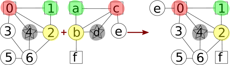
Figure 1. A toy example showing graph merge problem.

3. Iterative Global Structure Assisted Network Alignment

Figure 2 presents an overview of the proposed gsaNA algorithm. As illustrated in the figure, gsaNA is composed of three phases that are executed iteratively until a stable solution is found. Below we give a high-level overview of each of these phases, then in the following subsections, we discuss them in detail.

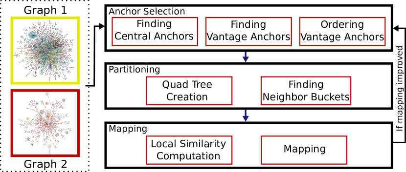
Figure 2. Overview of the gsaNA algorithm.

Anchor Selection:

Anchors are a small subset of vertices whose mappings are known. These anchors can be given by the user or they can be computed by gsaNA at the beginning. Our goal here is to identify a smaller subset of anchors, that we call vantage anchors, that can be used as reference points in the rest of the algorithm. This is done in three steps. First, for a given set of input anchors, gsaNA computes the central anchors in both graphs. Second, the remaining anchors are assigned to the closest central anchor. This helps us to classify anchor vertices. If two anchors are close to the same central anchor, then they cannot be good candidates to distinguish the vertices. gsaNA chooses vantage anchors from these assigned anchors. Finally, gsaNA pairs each vantage anchor with the most “distant ones”, orders and places them onto a unit circle to be used in the next phase. Figure 3 illustrates this process.

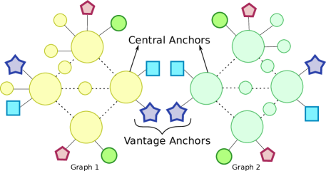
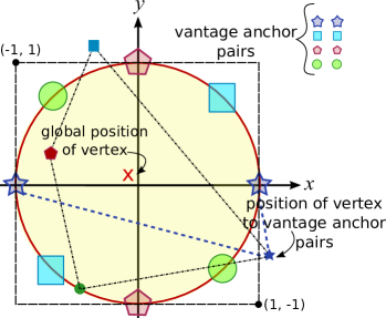
Figure 3. (a) Vantage anchor selection, (b) positioning of vantage anchors to unit circle, and vertex position computation.

Partitioning:

In this phase, vertices are partitioned into buckets on a $2D$ plane using their distances to the vantage anchors pairs. The intuition is that for a vertex $u$ to be mapped to a vertex $v$ in the other graph, their distances to the selected vantage anchor pairs should be similar. Hence, in this step, first, each vertex’s distances to vantage anchors are computed. Then, for each pair of vantage point position of the vertex on this $2D$ plane is computed. These positions define a polygon for each vertex. Finally, a single location is calculated by computing the centroid of this polygon. These final locations are used to partition the vertices into buckets. Due to the skewed and irregular structure of the graphs we expect the distribution of the positions will be skewed on this $2D$ plane. Therefore gsaNA partitions the plane with quad-trees (Finkel and Bentley, 1974).

Mapping:

The last phase of the algorithm is to compute pairwise similarity among the vertices of the two graphs that fell into the same bucket. Then compute a potentially partial mapping. The process is repeated for all non-empty buckets.

Iterations

The recall of gsaNA depends on the quality of the selected vantage anchors pairs. After computing a mapping, we have more information available for the alignment. By leveraging this information, we can recompute the vantage anchors, partition the vertices and map them. This way, we can choose better vantage anchors and decrease the number of false hits. We iteratively do these steps until the mapping is stable, i.e., it does not change more than a small fraction (we used 2% in our experiments). As initial anchors, we pick the highest scored mappings, and we double the number of anchors we use in each iteration, but we put an upper bound on that (1,000), and go back to initial anchors if we exceed that. Alg.  1 presents high-level pseudo-code of gsaNA.

$\mu\leftarrow\mu_{a}$, $\mu_{p}\leftarrow\varnothing$

$a\leftarrow|S_{1}|$

  $\triangleright$ Initialize $a$ as the size of the anchors set

$k\leftarrow 3$

  $\triangleright$ Initialize $k$ number of top similar vertices per vertex

$n\leftarrow 20$

  $\triangleright$ Initialize maximum number of iterations

$\epsilon\leftarrow 1.02$

  $\triangleright$ Minimum changes for next iteration

while $(n>0)$ and $(|\mu|\;/\;|\mu_{p}|>\epsilon)$  do

       $\mu_{p}\leftarrow\mu$

        $\triangleright$ Store current mapping in $\mu_{p}$

      

       $\triangleright$ Computation of shortest paths from seed anchors

       for each $u\in S_{1}$ do

            

             $\triangleright$ For each “new” seed anchor perform a BFS

             if  $\delta(u,.)$ is not computed before  then

                   $\delta(u,.)\leftarrow BFS(G_{1},u)$, $\delta(\mu[u],.)\leftarrow BFS(G_{2},\mu[u])$

                  

            

      

      $S_{C}\leftarrow$ findCentralAnchors$(G_{1},S_{1},\delta,1)$

       $S_{V}\leftarrow$ findVantageAnchors$(S_{1}\setminus S_{C},S_{C},\delta)$

       $O_{V}\leftarrow$pairAndOrder$(S_{V},\delta)$

      

      $Q\leftarrow$ QTree$((-1,1),(1,-1))$

       $T\leftarrow$ insertVertices$(V_{1}\cup V_{2},O_{V},Q,\delta)$

      

      $P\leftarrow$ topSimilars$(T,k,\sigma)$

       $\mu\leftarrow$ map$(P,\mu,\sigma)$

      

      

       $\triangleright$ Append highest similar vertices as new new anchors

      

      if $a>1000$ then

             $S_{1}=\{u:\mu_{a}[u]=v\}$

             $a\leftarrow|S_{1}|$

            

      

      for $i=1$ to $a$ do

             $S_{1}\cup\{u\}$, where $u\leftarrow\operatorname*{argmax}_{u\in V_{1}\setminus S_{1}}{\sigma(u,v)}$

            

      $a\leftarrow 2\times a$

       $n\leftarrow n-1$

      

return $\mu$

Algorithm 1 gsaNA($G_{1},G_{2},S_{1}$)

3.1. Anchor Selection

The size of the anchor set plays important role in gsaNA. We cannot request a complete mapping, but we need a few good anchors to start with. If an anchor set is not given by the user, we set $|S|=4\times\log(\max(|V_{1}|,|V_{2}|))$, and bootstrap the algorithm by finding $2\times|S|$ highest degree vertices in both graphs, and then by computing an initial mapping based on the similarity scores among them (see Section 3.4).

Given a centrality metric, we define set of central anchors $S_{C}$ as the $l=\log(|S|)$ vertices within the anchor set $S$ which have the highest centrality measures, and not “too close to each other”. Among many centrality measures (Freeman, 1978), we use the degree centrality. Alg. 2 presents the pseudo-code for this step.

 $\triangleright$ $\delta$ is a distance function, $t$ is distance threshold

 $\triangleright$ First find non-close anchors

$S^{\prime}\leftarrow\varnothing$

for each $u\in S$ do

       if $\forall v\in S^{\prime},\delta(u,v)>t$ then

             $S^{\prime}\leftarrow\{u\}$

            

      

$l\leftarrow\log(|S|)$

  $\triangleright$ Size limit of central anchors

 $\triangleright$ Get $l$ anchors with the highest degree

$C\leftarrow\varnothing$

for $i=1$ to $l$ do

       $C\leftarrow\{u\}$, where $u\leftarrow\operatorname*{argmax}_{u\in S^{\prime}\setminus C}|N[u]|$

      

return $C$

Algorithm 2 findCentralAnchors($G,S,\delta(\cdot,\cdot),t$)

gsaNA uses the central anchors to classify the rest of the anchors, where a subset of them is selected as vantage anchors. gsaNA uses the vantage anchors as the main reference points to partition the vertices of the graphs. Pseudo-code for finding vantage anchors is presented in Alg. 3. To identify them, for each non-central anchor, we first find the closest central anchor and assign non-central anchor to it. Then in order to evenly distribute vantage anchors over the graph, we limit the number of vantage anchors per central anchor, with the minimum number of assigned anchors to any central anchor. After, for each central anchor, among the assigned non-central anchors, we select the anchors that are farthest to it. Here, when needed, we break the ties by picking the anchor that is farthest than all other central anchors (this is not displayed in the algorithm).

$\forall c\in C,S_{V}^{\prime}[c]\leftarrow\varnothing$

  $\triangleright$ Initialize vantage anchor list

for each $u\in S^{\prime}$ do

       $S_{V}^{\prime}[c]\leftarrow\{u\}$, where $c\leftarrow\operatorname*{argmin}_{c\in C}\delta(u,c)$

      

$a\leftarrow\min_{c\in C}|S_{V}^{\prime}[c]|$

  $\triangleright$ limit num. of vantage anchors

$S_{V}\leftarrow\varnothing$

for each $c\in C$ do

       for $i=1$ to $a$ do

             $S_{V}\leftarrow\{u\}$, where $u\leftarrow\operatorname*{argmax}_{u\in S_{V}^{\prime}[c]}\delta(u,c)$

            

      

return $S_{V}$

Algorithm 3 findVantageAnchors($S^{\prime},C,\delta$)

Once anchors are assigned to the central anchors, we call Alg. 4 to pair the assigned anchors using the distance function $\delta$ and order them. Each vantage anchor is paired with the farthest vantage anchor. Then, one of the pairs is selected as the first pair. The rest of the pairs are ordered based on the distance of their first vertex to previous pair’s first vertex.

$cnt\leftarrow 0$

  $\triangleright$ Initialize counter for ordered pairs

for each $u\in S_{V}$ do

      

      $v\leftarrow\operatorname*{argmax}_{v\neq u\in S_{V}}\delta(u,v)$

       $O_{V}[cnt]\leftarrow[u,v]$

       $cnt\leftarrow cnt+1$

       $S_{V}\leftarrow S_{V}\setminus\{u,v\}$

       if $|S_{V}|\leq 1$ then

             break

            

      

for $i=2$ to $cnt$ do

       $j\leftarrow\operatorname*{argmin}_{i\leq j\leq cnt}\delta(O_{V}[i-1][1],O_{V}[j][1])$

       swap($O_{V}[i],O_{V}[j])$

return $O_{V}$

Algorithm 4 pairAndOrder($S_{V},\delta$)

3.2. Partitioning

The ordering of the vantage anchors are used to place them on a unit circle. The first pair is assumed to be “placed” at (1, 0) and (-1, 0), then second pair is placed on the unit circle with rotating $\pi/(|S|/2)$ in counter-clockwise (see Figure 3). Then, we compute the “position” of a vertex by placing the vertex as the corner of a right-angle triangle that is composed of the vertex and the vantage anchor pairs. So its distance to vantage anchors is scaled with the distance between vantage points and a point is computed using simple trigonometric functions. We repeat this process for every vantage anchor pairs. We then compute a final global position for the vertex as the centroid of the polygon defined by these locations as corners. The algorithm for this computation is displayed in Alg. 5. To partition vertices of the two input graphs, we simply compute a global position of each vertex using this algorithm, and then insert them into a quadtree. If a bucket exceeds pre-defined size limit, $B$, then that bucket is split into four. This continues until all of the vertices are inserted.

$\theta_{i}\leftarrow\theta\leftarrow\pi/|O_{V}|$

$poly\leftarrow\varnothing$

for $p\in O_{V}$ do

      

       $\triangleright$ distances between anchors and $u$

       $a\leftarrow\delta(u,p[0])$,   $b\leftarrow\delta(u,p[1])$,   $c\leftarrow\delta(p[0],p[1])$

      

       $\triangleright$ compute angle between $p[0]$ and $u$

       $\alpha\leftarrow arccos(a^{2}+c^{2}-b^{2})/(2\times ac)$

      

       $\triangleright$ compute $x$ and $y$ coordinates of $u$

       $x\leftarrow p[0].x-a\times cos(\alpha)$,    $y\leftarrow a\times sin(\alpha)$

      

      $poly.insert(Rotate((x,y),\theta_{i}))$

        $\triangleright$ rotate and insert into $l$

       $\theta_{i}\leftarrow rot+\theta$

      

return $Centroid(poly)$

Algorithm 5 getVertexPosition($u,O_{V},\delta$)

3.3. Mapping

Mapping is the third phase of our iterative algorithm, and the goal is to compute a mapping between vertices of the two graphs. As we have stated in Sec. 2, mapping step can be modeled as a maximum weighted bipartite graph matching (West, 2001) problem. However, since our overall algorithm is an iterative one, we will be sensitive and only finalize mappings that are most likely be the true mappings in each iteration, hoping that in further iterations, with more mapping information becomes available, similarity scores will reflect those and we can make better mappings. Our mapping algorithm (Alg. 6) starts with computing similarity scores for each vertex $v\in V_{2}$ in a non-empty bucket $B$ of the quadtree with vertex $u\in V_{1}$ that is either in the same bucket, or in one of the “neighboring” buckets. We check neighbor buckets to make sure that vertices are close to the border of the buckets are handled appropriately. After we identified top $k$ similar vertices (stored in $P[v]$), we compute a mapping, potentially a partial one, using Alg. 7. For each vertex, $u\in V_{2}$, we get $v\in V_{1}$ such that $v$ has the highest similarity score among the other candidates for $u$. Then we check the previously assigned mapping of $v$. If it had no mapping or previous mapping similarity score was less than what we have now, we mark $v$ as mapped to $u$. We repeat this procedure until there is no change in mapping. In short, our greedy mapping algorithm only considers the top $k$ best mappings, and only accept mapping both vertices agrees that their best “suitor” is each other.

 $\triangleright$ For each vertex keep a priority list with top $k$ elements.

$P[v]\leftarrow\varnothing$, for $\forall v\in V_{2}$

for each non-empty $B\in Q$ do

       for each $v\in B\wedge v\in V_{2}$ do

             for each $u\in Neig(B)\wedge u\in V_{1}$ do

                   $P[v].insert(u)$

                    $\triangleright$ Only keeps top $k$

                  

            

      

return $P$

Algorithm 6 topSimilars($Q,k,\sigma$)

$\mu_{p}\leftarrow\varnothing$

while $\mu_{p}\neq\mu$ do

       $\mu_{p}\leftarrow\mu$

       for each $u\in V_{2}$ where $P[u]\neq\varnothing$ do

             $v\leftarrow P[u].pop()$

              $\triangleright$ Pop the current best for $u$

             if $\mu[v]=\bot$ or $\sigma(v,u)>\sigma(v,\mu[v])$ then

                   $\mu[v]=u$

                  

            

      

return $\mu$

Algorithm 7 map($P,\mu,\sigma$)

3.4. Similarity Metrics

Our similarity score is composed of multiple components, some only depend on graph structure, some depends also on the additional metadata (types and attributes). Given two graphs $G_{1}$ and $G_{2}$ the similarity of two vertices, $u\in V_{1}$ and $v\in V_{2}$, our composite score is a simple average of six components as follows:

(2) $$\sigma(u,v)=\frac{\tau}{6}\times(\alpha+\Delta+\tau_{V}+\tau_{E}+C_{V}+C_{E})$$

where Table 2 lists the description of each component in this equation. Using these metrics we try to cover different graph characteristics which may help to increase final recall. Graph structure scores will be always available, and we include additional components when they are available. For example, when there is no additional metadata is available, our similarity score will reduce to average of two structural components:

(3) $$\sigma(u,v)=\frac{1}{2}\times(\alpha+\Delta).$$

Table 2. Components of the similarity function.

Symbol		Description
$\tau$	:	Type similarity
$\alpha$	:	Anchor similarity
$\Delta$	:	Relative degree distance (Koutra et al., 2013)
$\tau_{V}$	:	$\#Same/\#Total$ types of adjacent vertices
$\tau_{E}$	:	$\#Same/\#Total$ types of adjacent edges
$C_{V}$	:	Vertex attribute similarity
$C_{E}$	:	Edge attribute similarity

In a typed graph, types of the vertices are very important; for instance, one would not want to map a human in a graph with a shop in another graph. For this reason, we define type similarity, $\tau$, as a boolean metric (1 or 0), and it checks if the types of the vertices are the same or not.

Anchor similarity, $\alpha(u,v)$, is defined as the ratio of the number of common anchors among the neighbors of $u$ and $v$ to the total number of anchors in them. Formally, it is defined as:

(4) $$\alpha(u,v)=\frac{|\{w:w\in N_{1}[u]\wedge\mu[w]\in N_{2}[v]\wedge w\in S_{1}\}|}{|\{w:w\in N_{1}[u]\cup N_{2}[v]\wedge w\in S\}|}$$

We borrow the relative degree distance from (Koutra et al., 2013):

(5) $$\Delta(u,v)=\Big{(}1+\frac{2\times||N_{1}[u]|-|N_{2}[v]||}{||N_{1}[u]|+|N_{2}[v]||}\Big{)}^{-1}$$

The next two components takes type distributions of the neighboring vertices and edges into account. Let us define $tc[u,l]$ as the number of neighbors of $u$ of the type $l$, i.e., $tc[u,l]=|\{u^{\prime}:u^{\prime}\in N_{i}[u]\}\wedge t[u^{\prime}]=l\}|$. Then we define neighborhood vertex type similarity, $\tau_{V}(u,v)$, follows:

(6) $$\tau_{V}(u,v)=\frac{\sum\limits_{l\in L_{V}}\min(tc[u,l],tc[v,l])}{\sum\limits_{l\in L_{V}}\max(tc[u,l],tc[v,l])}$$

Neighborhood edge type similarity, $\tau_{E}$, is also defined in a similar way; we omit the equation for simplicity.

When the vertices and/or edges have attributes, we take those into account with attribute similarity metrics. Formally we define vertex attribute similarity, $C_{V}$, like a weighted, generalized Jaccard similarity, such that:

(7) $$C_{V}(u,v)=\frac{\sum_{c\in a[u]\cap a[v]}\min{w(c)}}{\sum_{c\in a[u]\cup a[v]}\max{w(c)}}$$

where $w(c)$ represents the weight of a non-numeric attribute.

When edge attributes are are non-numeric, we also define edge attribute similarity, $C_{E}$, very similar to Eq. 7. When attributes are numeric, we define $C_{E}$ as follows:

$$C_{E}(u,v)=\frac{\sum_{u^{\prime}\in N_{1}[u]}\sum_{v^{\prime}\in N_{2}[v]}close((u,u^{\prime}),(v,v^{\prime}))}{|N_{1}[u]|\times|N_{2}[v]|}$$

where $close(e,e^{\prime})$ is a boolean function, and it is 1 when value $|val(e)-val(e)|<\varepsilon$ for all numeric attributes, and 0 otherwise. Here, $val(e)$ denotes the value of edge attribute, and $\varepsilon$ is pre-determined threshold.

4. Related Work

Solution methods proposed in the literature for graph alignment can be roughly classified into four basic categories (Conte et al., 2004; Elmsallati et al., 2016): spectral methods (Singh et al., 2007; Liao et al., 2009; Patro and Kingsford, 2012; Neyshabur et al., 2013), graph structure similarity methods (Kuchaiev et al., 2010; Milenkovic et al., 2010; Memišević and Pržulj, 2012; Malod-Dognin and Pržulj, 2015; Aladağ and Erten, 2013), tree search or tabu search methods (Chindelevitch et al., 2013; Saraph and Milenković, 2014; Liu et al., 2007; Kpodjedo et al., 2014), and integer linear programming (ILP) methods (Klau, 2009; El-Kebir et al., 2011; Bayati et al., 2009). All of these works have scalability issues. Our algorithms leverage global graph structure and reduces the problem space and augment that with semantic information to alleviate most of the scalability issues.

As an example of spectral methods, IsoRank (Singh et al., 2007)—one of the earliest global alignment work in computational biology—suggests an eigenvalue problem that approximates the objective of finding the maximum common subgraph. After finding the vertex similarity matrix, IsoRank finds the alignment by solving the maximum weighted bipartite matching. IsoRank finds a 1/2-approximate matching using a greedy method, which aligns pair of vertices in the order of highest estimated similarity. IsoRank was extended to multiple networks in (Liao et al., 2009), where pairwise similarity matrices are computed and an iterative spectral clustering is used to output set of vertices, one from each network, that aligns with each other. It is noted that it cannot handle more than five networks.

In (Klau, 2009), named as Klau in our experiments, the problem of finding the mapping with the maximum score is posed as an integer quadratic program. It is solved by an integer linear programming (ILP) formulation via a sequence of max-weight matching problems. Authors use Lagrangian relaxation to solve this problem approximately in a more reasonable time. However, the ILP based solutions will not scale to larger problem sizes.

NetAlign (Bayati et al., 2009) formulates the network alignment problem as an integer quadratic programming problem to maximize the number of “squares”. A near-optimal solution is obtained by finding the maximum a posteriori assignment using belief propagation heuristic and message-passing algorithms which yield near optimal results in practice. Another message passing network alignment algorithm on top of belief propagation is proposed by Bradde et al. (Bradde et al., 2010). In (Koutra et al., 2013) Koutra et al. propose to align two bipartite graphs with a fast projected gradient descent algorithm which exploits the structural properties of the graphs.

In a more recent work, Zhang et al. propose Final (Zhang and Tong, 2016) to solve attributed network alignment problem. Final extends the concept of IsoRank  (Singh et al., 2007), and make it capable to benefit from attribute information of the vertices and edges to solve this problem. In addition to graph’s vertex, edge and attribute sets Final adds an optional input called prior knowledge matrix (H) in which each entry gives likelihood to align two vertices. Final is one of the most recent works which solves attributed graph alignment problem and outperforms (Singh et al., 2007; Klau, 2009; Bayati et al., 2009; Koutra et al., 2013).

Table 3. Properties of the datasets. $\langle|N[x]|\rangle$ represents average vertex degree, and $|\mu|$ represent the size of ground truth mapping.

Data Set	$\boldsymbol{|V|}$	$\boldsymbol{|E|}$	$\boldsymbol{\langle|N[x]|\rangle}$	$\boldsymbol{\max(|N[x]|)}$	$\boldsymbol{|N[x]|<3}$		$\boldsymbol{|\mu|}$	$\boldsymbol{|L_{V}|}$	$\boldsymbol{|L_{E}|}$	$\boldsymbol{|S_{1}|}$	$\boldsymbol{A_{V}}$	$\boldsymbol{A_{E}}$
Douban-Online	3,906	16,328	4.18	124	1,467	(38%)	1,118	538	2	48	✗	✗
Douban-Offline	1,118	3,022	2.71	38	638	(57%)
Facebook-1	4,038	88,234	21.86	696	173	(4%)	4,011	5	1	48	✗	✗
Facebook-2	4,438	79,411	17.89	615	196	(4%)
Lastfm	15,436	32,638	2.11	1,952	13,961	(91%)	452	3	3	56	✓	✗
Flickr	12,974	32,298	2.49	1,736	10,383	(81%)
Myspace	10,733	21,767	2.03	326	10,120	(94%)	267	3	3	54	✓	✗
Flickr	6,714	14,666	2.18	1,278	5,836	(87%)
DBLP-17 (0)	59,006	665,800	11.28	2,322	3,098	(5%)	27,029	1	1	68	✓	✓
DBLP-14 (0)	43,936	368,983	8.40	1,782	3,248	(7%)
DBLP-17 (1)	118,012	1,287,928	10.91	2,322	7,086	(6%)	60,902	1	1	68	✓	✓
DBLP-14 (1)	87,873	705,725	8.03	1,782	7,230	(8%)
DBLP-17 (2)	236,025	2,232,274	9.46	2,322	17,364	(7%)	130,786	1	1	72	✓	✓
DBLP-14 (2)	175,746	1,322,910	7.43	1,782	17,688	(10%)
DBLP-17 (3)	491,719	4,089,071	8.31	2,322	51,035	(10%)	294,531	1	1	75	✓	✓
DBLP-14 (3)	366,137	2,542,331	6.94	1,782	46,853	(13%)
DBLP-17 (4)	983,438	6,685,519	6.80	2,322	148,408	(15%)	649,500	1	1	79	✓	✓
DBLP-14 (4)	732,275	4,268,145	5.83	1,782	128,641	(18%)
DBLP-17	1,966,877	9,059,634	4.61	2,322	616,386	(31%)
DBLP-14	1,464,539	5,906,792	4.03	1,782	491,206	(34%)	1,440,379	1	1	83	✓	✓
DBLP-15	1,620,196	6,828,586	4.22	2,168	528,949	(33%)	1,601,443	1	1	83	✓	✓
DBLP-16	1,783,746	7,841,210	4.40	2,149	571,703	(32%)	1,772,129	1	1	83	✓	✓

5. Experimental Evaluation

In this section, we first present several experiments in order to identify the performance trade-offs of the parameters of gsaNA.

We then compare the performance of proposed gsaNA algorithm gsaNA against four state-of-the-art mapping algorithms: IsoRank (Singh et al., 2007), Klau (Klau, 2009), NetAlign (Bayati et al., 2009), and Final (Zhang and Tong, 2016), each briefly described in the previous section. We also present performance of these algorithms and gsaNA when there are errors in the graph structure or in the attributes. In our experiments we used Matlab implementations of these algorithms  (Zhang and Tong, 2017; Netalign, 2017).

Experiments were carried out on machine that has 2 16-core Intel Xeon E5-2683 2.10GHz processors, 512GB of memory, 1TB disk space, running Ubuntu GNU/Linux with kernel 4.8.0. gsaNA is implemented in C++ and complied with GCC 5.4.

5.1. Dataset

We use real-world graphs obtained from (Zhang and Tong, 2017; of Trier, 2017; Demaine and Hajiaghayi, 2017). We also generated different size of DBLP (of Trier, 2017) graphs. The properties of graphs are listed in Table 3 and we briefly describe them below.

Douban Online-Offline (Zhang and Tong, 2017): These two graphs are extracted subnetworks of the original dataset (Zhong et al., 2012). The original dataset contains $50k$ users and $5M$ edges. Both networks are constructed using users’ co-occurrences in social gatherings. In (Zhang and Tong, 2016) people are treated as, (i)  ’contacts’ of each other if the cardinality of their common event participations is between ten and twenty times, (ii)  ’friends’ if the cardinality of their common event participation is greater than 20. The constructed offline and online network has 1,118 and 3,906 vertices respectively. The location of a user is used as the vertex attribute, and ’contacts’/’friends’ as the edge attribute. In (Zhang and Tong, 2016) degree similarity is used to construct prior preference matrix $H$.

Flickr-Lastfm (Zhang and Tong, 2017): These two graphs are extracted subnetworks of the original versions (Zhang et al., 2015). The original versions contain $216K$, $136K$ users and $9M$, $1.7M$ edges respectively. (Zhang et al., 2015; Zhang and Tong, 2016) construct an alignment scenario for original dataset by subtracting a small subnetwork for their ground-truth. The two subnetworks have 12,974 nodes and 15,436 nodes, respectively. In extracted subnetworks, the gender of a user (male, female, unknown) considered as the vertex attribute. (Zhang et al., 2015; Zhang and Tong, 2016) sort nodes by their PageRank scores to label vertices as “opinion leaders”, “middle class”, and “ordinary users”. Edges are attributed by the level of people they connect to (e.g., leader with leader). The user name similarity is used to construct prior preference matrix $H$.

Flickr-Myspace (Zhang and Tong, 2017): These two graphs are extracted subnetworks of the original dataset (Zhang et al., 2015). Original datasets contains $216K$, $854K$ users and $9M$, $6.5M$ edges respectively. (Zhang et al., 2015; Zhang and Tong, 2016) construct an alignment scenario for original dataset by subtracting a small subnetwork for their ground-truth. The two subnetworks have 6,714 nodes and 10,733 nodes, respectively. The vertex and edge attributes computed using the same process described for Flickr-Lastfm.

Facebook-Facebook: We use Snap’s (Leskovec and Krevl, 2017) facebook-ego graph. First, we randomly permute this graph and remove 20% of the edges. Then, we add 10% new vertices and randomly add 10% edges to create the second network.

DBLP (2014-2017): We downloaded consecutive years of DBLP graphs from 2014 (Demaine and Hajiaghayi, 2017) to 2017 (of Trier, 2017). The ground-truth between these two graphs is created using authors’ key element. Vertices are authors and two authors have an edge if they have co-authored information. For each publication, DBLP records a cross-ref like ‘conf/iccS/2010’. We use this cross-ref information to create vertex attributes by splitting a cross-ref by ‘/’ and unionizing initial character of each word as the vertex attribute. Edge attribute between two vertices is the mean of the publication years of co-authored papers between two authors. The other DBLP graphs listed in Table 3, the ones with suffixes (0) through (4), are smaller subgraphs of the original DBLP graph, centered around highest degree vertex.

5.2. gsaNA: Structure Assisted Partitioning

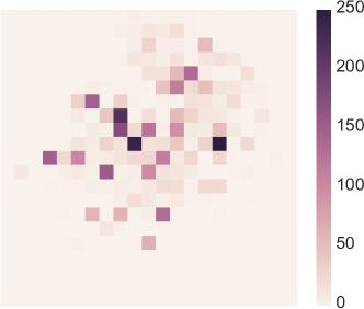
(a) Facebook

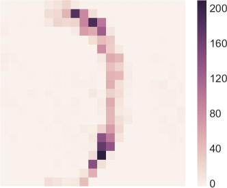
(b) Douban

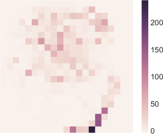
(c) Flickr-lastfm

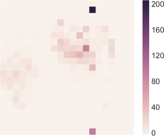
(d) Flickr-Myspace

Figure 4. Density Heat Maps

Figure 4 shows the density heat maps of four real-world datasets after the vertices are positioned onto $2D$ using the techniques presented in Section 3.2. Each of the sub-figures presents a square from $(-1,1)$ to $(1,-1)$. Vertices’ coordinates are found using Alg. 5. We have partitioned this space as a uniform grid with bucket sizes of $0.1\times 0.1$, then counted the number of vertices in each bucket. Darker color represents higher number of vertices in that bucket.

The first thing we observe from Figure 4 is that our partitioning algorithm is working, that is, it enables us to partition the vertices into different buckets by mapping them into a $2D$ and then partitioning that plane with space partitioning techniques. As expected, uniform density, in other words, load-balance partitioning of buckets, is almost always impossible because of the skewness of the real-world graphs. Therefore instead of using a grid-like partitioning, we use quadtree  (Finkel and Bentley, 1974) based partitioning.

5.3. gsaNA: Scope of Bucket Comparison

In Table 4 we compare the performance of gsaNA under two settings: first, during mapping gsaNA only considers vertices in the same bucket; second gsaNA looks neighbors of each bucket for possible mappings. In order to quantify this, we define Hit Count as the ratio of the number of $\mu[v]=u$ mappings considered (i.e., gsaNA computed a similarity score between $u$ and $v$, it may or may not map them) to the number of such true mappings.

For the settings, we measure the recall, hit count and gain for alignment of DBLP(2014-2016) vs DBLP(2017) graphs. We define gain as the ratio of the pair of vertices which we do not compute a similarity score to the total pair of vertices.

	DBLP Graphs
	$14$ vs $17$	$15$ vs $17$	$16$ vs $17$
	Without Neighbors
Recall	31%	32%	41%
Hit Count	40%	55%	63%
Gain	$\approx 99.97$ %	$\approx 99.98$%	$\approx 99.98$%
	With Neighbors
Recall	47%	58%	66%
Hit Count	88%	92%	95%
Gain	$\approx 99.85$ %	$\approx 99.85$%	$\approx 99.86$%

Table 4. Scope of bucket comparisons.

We have following observations, first, the quality of mapping, i.e. recall, improves with the decrease in the year differences between two graphs. This is an expected result, for example, 2016 graph is more similar to 2017 graph than 2014 graph. Second, the hit count rate decreases almost half when gsaNA only considers vertices within the same bucket. A similar, though not as much, decrease is also observed in recall. Third, hit count is sufficiently high for the second case. Forth, the gain is very high in both cases, i.e., gsaNA approximately compares only $1/5000$ of possible vertex pairs in the first case, and only $1/1000$ in the second case. Based on these results, we set the default of gsaNA to consider neighbors of each bucket for possible mappings.

5.4. gsaNA: Effects of Bucket Size

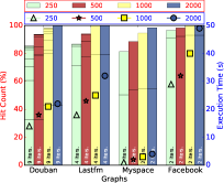
(a) Hit Count: $1^{st}$ set of Graphs

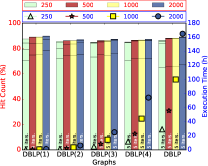
(b) Hit Count: $2^{nd}$ set of Graphs

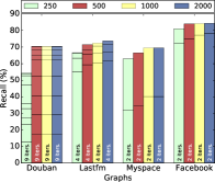
(c) Recall: $1^{st}$ set of Graphs

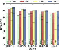
(d) Recall: $2^{nd}$ set of Graphs

Figure 5. Figures 5(a) and 5(b) plot the Hit Count (left axis) and Execution Time (right axis), and Figures 5(c) and 5(d) plot the Recall, as a function of different graph and bucket sizes. Each bar represents a different bucket size. Number of iterations of gsaNA for each instance is printed at the bottom of each bar, and hit count or recall at each iteration is depicted as stacked results.

In this section, we study the effects of bucket size on the recall and execution time. Figures 5(a) and 5(b) plot the Hit Count and execution time of gsaNA as a function of bucket and graph size. We observe from Figures 5(a) and 5(b) that run time increase is sub-linear in the size of buckets within each dataset. Quad-tree style partitioning is one of the key factors that determine the number of comparisons which affects the run time. When we double the bucket size the number of buckets and average number of vertices per bucket does not double. This explains the sub-linear trend with respect to the bucket sizes. We observe from Figure 5(b) that number of edges affects runtime because it affects the complexity of our similarity function. For instance, running time increases in average about $5\times$ between DBLP(0) and DBLP(1) graphs and $2.3\times$ between DBLP(4) DBLP, while the number of edges increase in average about $1.9\times$ and $1.4\times$ respectively. We also observe from Figures 5(a) and 5(b) that Hit Count slightly increases with increasing bucket sizes.

Briefly, recall is the ratio of the correct mapping found by gsaNA to the number of ground truth mapping. Figures 5(c) and  5(d) show the trend in recall as a function of different bucket sizes for different graphs. From the figures, we observe that increasing the bucket size increases the recall, but there is a diminishing return as expected. Recall increases about $8\%$ on the average with increasing bucket sizes from $250$ to $2000$ and only $4\%$ when bucket sizes from $500$ to $2000$. Based on these results we picked bucket size $500$ as our default for further experiments.

5.5. Comparison against state-of-the-art

Here, we compare our proposed algorithm, gsaNA, with four state-of-the-art mapping algorithms: IsoRank (Singh et al., 2007), Klau (Klau, 2009), NetAlign (Bayati et al., 2009), and Final (Zhang and Tong, 2016).

In the experiments presented in Section 5.5.1 to 5.5.4 (Figures 6(a)-7(b) respectively) we also take additional metadata information, such as vertex and edge attributes, types, etc., whenever it exist. NetAlign (Bayati et al., 2005) and Klau (Klau, 2009) require an additional bipartite graph, representing the similarity scores between two input graphs’ vertices. Final (Zhang and Tong, 2016)’s goal is to leverage the additional metadata information and improve IsoRank (Singh et al., 2007). Therefore, in these experiments Final’s (Zhang and Tong, 2016) prior preference matrix H is used for Douban, Flickr-Lastfm and Flickr-Myspace graphs for all other algorithms. We have used $H$ as gsaNA’s $C_{V}$ for Flickr-Lastfm and Flickr-Myspace graphs, since they reflected vertex attribute similarity, and vertex attributes were not provided separately. In Facebook, each vertex considered as possible mapping between top similar (computed as $\sigma=\tau\times\Delta$, see Section 3.4) $s$ vertices, where $s$ is randomly selected number in the range of $[5,15]$.

In DBLP(0), first a similarity matrix is generated using $C_{V}$ and then all elements smaller than 0.9 set as 0. Both for Facebook and DBLP(0) after deciding possible mappings we have also added ground truth for not to miss any information. In order to be fair, and help to improve IsoRank’s result, we also set its similarity matrix’s elements corresponding to 0 elements in H as 0 as well.

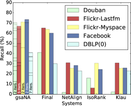
(a) Anchors are not known

(b) Anchors are known

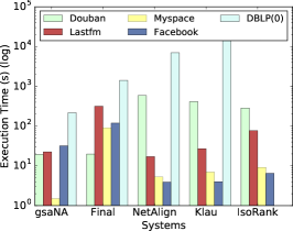
(c) Execution Time

Figure 6. Figures 6(a) to 6(b) plot the Recall of the systems under conveyed scenarios. Figure 6(c) plots the Execution Time. In each plot (left axis) represents Recall or Execution Time . Each bar represents a different graph.

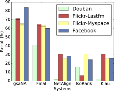
(a) Structural Noise

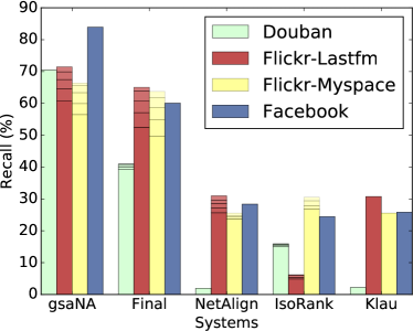
(b) Attributed Noise

Figure 7. Recall under noise. In each plot (left axis) represents Recall or Execution Time . Each bar represents a different graph.

5.5.1. Anchors are not known

Figure 6(a) plots the results where we assume anchors are not given to gsaNA by the user, and gsaNA computes anchors as described in Sec. 3.1. As seen in the figure, gsaNA outperforms all of the algorithms in terms of recall. On the average, gsaNA produces about $1.3\times$ better recall than Final, $9\times$ better recall than NetAlign, $5\times$ better recall than IsoRank and $8\times$ better recall than Klau. However, NetAlign and Klau performs really poor on Douban dataset, therefore if we omit this dataset gsaNA produces $2.3\times$ and $2.4\times$ better results than NetAlign and Klau, respectively.

5.5.2. Anchors are known

Figure 6(b) presents the results where the anchor set is given by the user. We set these anchors’ similarity score as 1.0 in all the other algorithms we compare too. We observe that gsaNA’s recall increases in Facebook and DBLP(0) graphs because wrong initial anchor mapping are corrected. However, Flickr-Myspace graphs’ recall slightly decreases gsaNA produces about $1.4\times$ better recall than Final, $9\times$ better recall than NetAlign, $5\times$ better recall than IsoRank and $\approx 8\times$ better recall than Klau. Same as previous experiment if we omit Douban dataset gsaNA produces $2.6\times$ and $2.7\times$ better results than NetAlign and Klau, respectively.

5.5.3. Execution Time

Figure 6(c) displays the execution time results, in log-scale, of the algorithms we compare. In this figure, the pre-processing time of computing similarity bipartite graph for NetAlign and Klau and $H$ matrix for Final is not included (we have directly used the $H$ matrix provided with Final implementation). We would like to note that, computation of those similarity scores requires a significant time. Another point we need to remind, gsaNA is written in C++ while the other algorithms are implemented in Matlab. Hence, it may not be appropriate to compare individual absolute results, but still these results should be good to provide some insights to trends of the execution time.

For small graphs, all algorithms are “fast enough” to use in practice. However, for DBLP(0), which the smallest of our DBLP graphs, as you can see other algorithms becomes orders of magnitudes slower. gsaNA can solve our largest DBLP graph, 32 times larger than DBLP(0), almost with same time they take for DBLP(0).

5.5.4. Effect of Errors

In Figure 7(a) we present results when there is structural error in the input graphs. We randomly remove 5%, 10%, 15% and 20% of the edges from both graphs, then for each case we re-run the systems. Since we observed only small amount of change in the results, and recall of mapping decreased with increasing error rate, in all experiments, we simply plotted them as a stacked bar results, that is there are 4 horizontal lines in each bar depicting 5%, 10%, 15% and 20% error, from top to bottom. We expect, at some point, gsaNA will be effected from structural error because eventually shortest paths are going to change, and hence partitioning. However, as seen in the figure, removing edges up to 20% did not significantly change the partitioning because the results doesn’t significantly changed, i.e. still gsaNA has good hit count ratio.

In Figure 7(b) we present results when there are errors in attributes. Since we had used $H$ matrices provided by Final as our attribute similarity, basically we randomly changed 5%, 10%, 15% and 20% of the non-zero elements of $H$. And for each case we re-run all the algorithms, except Klau (Klau, 2009), since the errors in attributes do not affect it. As expected other systems’ recalls, including that of gsaNA, decrease when we increase the noise. We also observe that interestingly while removing edges randomly doesn’t affect IsoRank, adding noise to its similarity matrix changes its final recall. This experiment, as expected showed that largest changes in the recall were in gsaNA and Final, especially in Flickr-Lastfm and Flickr-Myspace data sets, since those are the algorithms that incorporates the attribute similarity.

6. Conclusion

We have developed an iterative graph alignment framework called gsaNA, which leverages the global structure-based vertex positioning technique to reduce the problem size, and produces high quality alignments that outperforms the state-of-the-art. As the graph sizes increases, the runtime performance of the proposed algorithm becomes more pronounced, and becomes order of magnitudes faster than the existing algorithms, without a significant decrease in the performance. As a future work, our goal is parallelize gsaNA to take advantage of multi-node and/or multi-core architectures. Many parts of the algorithm, like initial distance computations from multiple anchors, and pairwise similarity computation, which are the most two time consuming part of the gsaNA, can be easily parallelized. We also would like to explore techniques to extend gsaNA to solve multi graph alignment problem.

References

- (1)
- Aladağ and Erten (2013) Ahmet E Aladağ and Cesim Erten. 2013. SPINAL: scalable protein interaction network alignment. Bioinformatics 29, 7 (2013), 917–924.
- Bayati et al. (2009) Mohsen Bayati, Margot Gerritsen, David F Gleich, Amin Saberi, and Ying Wang. 2009. Algorithms for large, sparse network alignment problems. In IEEE International Conference on Data Mining (ICDM). 705–710.
- Bayati et al. (2005) Mohsen Bayati, Devavrat Shah, and Mayank Sharma. 2005. Maximum weight matching via max-product belief propagation. In International Symposium on Information Theory (ISIT). 1763–1767.
- Bradde et al. (2010) Serena Bradde, Alfredo Braunstein, Hamed Mahmoudi, Francesca Tria, Martin Weigt, and Riccardo Zecchina. 2010. Aligning graphs and finding substructures by a cavity approach. EPL (Europhysics Letters) 89, 3 (2010), 37009.
- Chindelevitch et al. (2013) Leonid Chindelevitch, Cheng-Yu Ma, Chung-Shou Liao, and Bonnie Berger. 2013. Optimizing a global alignment of protein interaction networks. Bioinformatics (2013), btt486.
- Conte et al. (2004) Donatello Conte, Pasquale Foggia, Carlo Sansone, and Mario Vento. 2004. Thirty years of graph matching in pattern recognition. International journal of pattern recognition and artificial intelligence 18, 03 (2004), 265–298.
- Demaine and Hajiaghayi (2017) Erik Demaine and MohammadTaghi Hajiaghayi. 2017. BigDND: Big Dynamic Network Data. http://projects.csail.mit.edu/dnd/. (2017).
- El-Kebir et al. (2011) Mohammed El-Kebir, Jaap Heringa, and Gunnar W Klau. 2011. Lagrangian relaxation applied to sparse global network alignment. In IAPR International Conference on Pattern Recognition in Bioinformatics. Springer, 225–236.
- Elmsallati et al. (2016) Ahed Elmsallati, Connor Clark, and Jugal Kalita. 2016. Global Alignment of Protein-Protein Interaction Networks: A Survey. IEEE Transactions on Computational Biology and Bioinformatics 13, 4 (2016), 689–705.
- Finkel and Bentley (1974) Raphael A Finkel and Jon Louis Bentley. 1974. Quad trees a data structure for retrieval on composite keys. Acta informatica 4, 1 (1974), 1–9.
- Freeman (1978) Linton C. Freeman. 1978. Centrality in social networks conceptual clarification. Social Networks 1, 3 (1978), 215 – 239.
- Ito et al. (2001) Takashi Ito, Tomoko Chiba, Ritsuko Ozawa, Mikio Yoshida, Masahira Hattori, and Yoshiyuki Sakaki. 2001. A comprehensive two-hybrid analysis to explore the yeast protein interactome. Proceedings of the National Academy of Sciences 98, 8 (2001), 4569–4574.
- Jafar et al. (2011) Syed A Jafar et al. 2011. Interference alignment A new look at signal dimensions in a communication network. Foundations and Trends® in Communications and Information Theory 7, 1 (2011), 1–134.
- Klau (2009) Gunnar W. Klau. 2009. A new graph-based method for pairwise global network alignment. BMC Bioinformatics 10, 1 (2009), S59.
- Koutra et al. (2013) Danai Koutra, Hanghang Tong, and David Lubensky. 2013. Big-align: Fast bipartite graph alignment. In IEEE International Conference on Data Mining (ICDM). 389–398.
- Kpodjedo et al. (2014) Segla Kpodjedo, Philippe Galinier, and Giulio Antoniol. 2014. Using local similarity measures to efficiently address approximate graph matching. Discrete Applied Mathematics 164 (2014), 161–177.
- Kuchaiev et al. (2010) Oleksii Kuchaiev, Tijana Milenković, Vesna Memišević, Wayne Hayes, and Nataša Pržulj. 2010. Topological network alignment uncovers biological function and phylogeny. Journal of the Royal Society Interface 7, 50 (2010), 1341–1354.
- Leskovec and Krevl (2017) Jure Leskovec and Andrej Krevl. 2017. SNAP Datasets: Stanford Large Network Dataset Collection. http://snap.stanford.edu/data. (2017).
- Liao et al. (2009) Chung-Shou Liao, Kanghao Lu, Michael Baym, Rohit Singh, and Bonnie Berger. 2009. IsoRankN: spectral methods for global alignment of multiple protein networks. Bioinformatics 25, 12 (2009), i253–i258.
- Liu et al. (2007) Dasheng Liu, Kay Chen Tan, Chi Keong Goh, and Weng Khuen Ho. 2007. A multiobjective memetic algorithm based on particle swarm optimization. IEEE Transactions on Systems, Man, and Cybernetics, Part B 37 (2007), 42–50.
- Malod-Dognin and Pržulj (2015) Noël Malod-Dognin and Nataša Pržulj. 2015. L-GRAAL: Lagrangian graphlet-based network aligner. Bioinformatics (2015), btv130.
- Melnik et al. (2002) Sergey Melnik, Hector Garcia-Molina, and Erhard Rahm. 2002. Similarity flooding: A versatile graph matching algorithm and its application to schema matching. In IEEE International Conference on Data Engineering (ICDE). 117–128.
- Memišević and Pržulj (2012) Vesna Memišević and Nataša Pržulj. 2012. C-GRAAL: C ommon-neighbors-based global GRA ph AL ignment of biological networks. Integrative Biology 4, 7 (2012), 734–743.
- Milenkovic et al. (2010) Tijana Milenkovic, Weng Leong Ng, Wayne Hayes, and Natasa Przulj. 2010. Optimal network alignment with graphlet degree vectors. Cancer informatics 9 (2010), 121.
- Netalign (2017) Netalign 2017. netalign : Network Alignment codes. https://www.cs.purdue.edu/homes/dgleich/codes/netalign/. (2017).
- Neyshabur et al. (2013) Behnam Neyshabur, Ahmadreza Khadem, Somaye Hashemifar, and Seyed Shahriar Arab. 2013. NETAL: a new graph-based method for global alignment of protein–protein interaction networks. Bioinformatics 29, 13 (2013), 1654–1662.
- of Trier (2017) University of Trier. 2017. DBLP: Computer Science Bibliography. http://dblp.dagstuhl.de/xml/release/. (2017).
- Patro and Kingsford (2012) Rob Patro and Carl Kingsford. 2012. Global network alignment using multiscale spectral signatures. Bioinformatics 28, 23 (2012), 3105–3114.
- Saraph and Milenković (2014) Vikram Saraph and Tijana Milenković. 2014. MAGNA: maximizing accuracy in global network alignment. Bioinformatics 30, 20 (2014), 2931–2940.
- Singh et al. (2007) Rohit Singh, Jinbo Xu, and Bonnie Berger. 2007. Pairwise global alignment of protein interaction networks by matching neighborhood topology. In Annual International Conference on Research in Computational Molecular Biology. 16–31.
- Uetz et al. (2000) Peter Uetz, Loic Giot, Gerard Cagney, Traci A. Mansfield, et al. 2000. A comprehensive analysis of protein–protein interactions in Saccharomyces cerevisiae. Nature 403, 6770 (2000), 623–627.
- Viola and Wells III (1997) Paul Viola and William M Wells III. 1997. Alignment by maximization of mutual information. International journal of computer vision 24, 2 (1997), 137–154.
- West (2001) Douglas B. West. 2001. Introduction to graph theory. Pearson.
- Zhang and Tong (2016) Si Zhang and Hanghang Tong. 2016. FINAL: Fast Attributed Network Alignment. In ACM International Conference on Knowledge Discovery and Data mining. 1345–1354.
- Zhang and Tong (2017) Si Zhang and Hanghang Tong. 2017. FINAL: Fast Attributed Network Alignment. https://github.com/maffia92/FINAL-network-alignment-KDD16. (2017).
- Zhang et al. (2015) Yutao Zhang, Jie Tang, Zhilin Yang, Jian Pei, and Philip S. Yu. 2015. COSNET: Connecting Heterogeneous Social Networks with Local and Global Consistency. In ACM International Conference on Knowledge Discovery and Data mining. 1485–1494.
- Zhong et al. (2012) Erheng Zhong, Wei Fan, Junwei Wang, Lei Xiao, and Yong Li. 2012. ComSoc: Adaptive Transfer of User Behaviors over Composite Social Network. In ACM International Conference on Knowledge Discovery and Data mining. 696–704.