Model Structural Inference using LDOs \authorheadA.M. DeGennaro, N.M. Urban, B.T. Nadiga, & T. Haut \corrauthor[1]Anthony M. DeGennaro \corremailadegennaro@bnl.gov \corraddressComputational Science Initiative, Brookhaven National Laboratory, Upton, NY, 11973
mm/dd/yyyy
Model Structural Inference using Local Dynamic Operators
Abstract
This paper focuses on the problem of quantifying the effects of model-structure uncertainty in the context of time-evolving dynamical systems. This is motivated by multi-model uncertainty in computer physics simulations: developers often make different modeling choices in numerical approximations and process simplifications, leading to different numerical codes that ostensibly represent the same underlying dynamics. We consider model-structure inference as a two-step methodology: the first step is to perform system identification on numerical codes for which it is possible to observe the full state; the second step is structural uncertainty quantification (UQ), in which the goal is to search candidate models “close” to the numerical code surrogates for those that best match a quantity-of-interest (QOI) from some empirical dataset. Specifically, we: (1) define a discrete, local representation of the structure of a partial differential equation, which we refer to as the “local dynamical operator” (LDO); (2) identify model structure non-intrusively from numerical code output; (3) non-intrusively construct a reduced order model (ROM) of the numerical model through POD-DEIM-Galerkin projection; (4) perturb the ROM dynamics to approximate the behavior of alternate model structures; and (5) apply Bayesian inference and energy conservation laws to calibrate a LDO to a given QOI. We demonstrate these techniques using the two-dimensional rotating shallow water (RSW) equations as an example system.
keywords:
Structural Uncertainty Quantification, Model Form Uncertainty Quantification, Low-Dimensional Modeling, Local Dynamic Operator, Equation Learning, Model Inference1 Introduction
For predictive modeling of a complex dynamical system to be successful, it is critical to be able to comprehensively account for the full range of uncertainties that influence the system. Such uncertainties are found in initial conditions, boundary and/or operating conditions, governing parameters, computational approaches, and model-form. The last of these stems from an imperfect or incomplete description of the full range of dynamics and/or physics that underlies the complex behavior exhibited by the system of interest.
While model-form uncertainty is an active area of research, it is at present less studied than other forms of uncertainty. A main approach to quantifying it has relied on multi-model ensembles or ensembles of opportunity wherein models from different modeling groups are analysed statistically in an a posteriori fashion [1, 2, 3]. However, this approach typically does not give representation to all plausible structural differences: there are many hypothetical model structures, representing reasonable physical/empirical assumptions that in principle could be implemented and studied, but have not been. A multi-model ensemble approach therefore generally cannot quantify the full range of possible structural uncertainties in a dynamical system, since it studies only a discrete subset of model structures.
In contrast, parametric uncertainty is a well-studied canonical problem, with correspondingly well-developed techniques for quantification. Motivated by this observation, one might wonder if it is possible to effectively re-cast certain problems in structural uncertainty as equivalent problems in parametric uncertainty, for which a broad and powerful set of tools exist. This is a main component of the approach we propose in this paper: we seek to encapsulate plausible differences in model structure in some parametric approximation of the governing dynamics. In this scheme, different models are represented by different locations in some parameter space.
In order to specify the nature of this structure-parameterization, we begin by making the crucial assumption that the field dynamics may be well approximated by a functional relationship which is local and spatio-temporally invariant. By local, we mean that the field evolution in time at a particular point in space is governed only by the field values in a nearby neighborhood; by spatio-temporal invariance, we mean that the mapping that describes this evolution is the same for all points in space at all times.
Given these assumptions, the discretized dynamics can be described by what we will refer to as a local dynamic operator (LDO), which is simply a functional relationship between spatially-local field values that approximates the discretized governing field dynamics at a spatial point. For example, if the governing equations are hyperbolic, then the LDO is a function that takes field values in a spatially-local neighborhood of a center point and outputs the field value at that center point, one time step forward in time. Note that there is an attractive consequence of our assumptions of locality and spatio-temporal invariance with respect to system identification: if we wish to infer a LDO from numerical/experimental data, access to the full global state vector is not strictly required. We may simply collect data from a subset of spatial points (together with the appropriate surrounding local neighborhoods). This is a notable advantage relative to a system identification technique that would require the full global state vector (e.g., POD).
As all of the dynamics are encoded in the LDO, any structural uncertainties are as well. Furthermore, if we can design the LDO to be a weighted sum of different elementary functions of the local field values, then the relevant structural uncertainties manifest themselves as uncertainties in the values of the weights, which are simply parameters. This is a sketch of the process by which we convert structural uncertainties to parametric ones.
Having formalized a means to parameterize model structure, all of the machinery of parametric uncertainty quantification (UQ) is available to study the structural uncertainty in model dynamics, which we propose doing in the following two-step process. First, we show how we may learn model structure (i.e., LDO parameters) non-intrusively using statistical function approximation techniques (e.g., least-squares regression). Second, we show how Monte Carlo sampling may be used to perturb the LDO parameters, giving us a systematic, probabilistic means for performing model structural UQ.
Without any other constraints, the number of LDO parameters can be prohibitively large for the second step of our process: Monte Carlo sampling in a high-dimensional parameter space is a challenge. We explore two methods for alleviating this. First, we explicitly assume that the user has partial prior knowledge about the physics involved, and we use this knowledge to constrain the LDO parameter space and reduce its dimensionality. In doing this, we are making our mehod a “greybox”, and as such, our approach is not aimed at users who desire a purely data-driven, completely physics-agnostic approach. Instead, we are targeting those users who have a combination of both some prior knowledge and some data, and we are proposing a framework to effectively join the two. The second avenue that we investigate for reducing computational expense involves building reduced-order models (ROMs) of the LDO-parameterized dynamics, using POD-DEIM-Galerkin projection.
The envisioned practical application for these ideas is quantification/learning of subgrid physics. The motivation here is that several numerical models exist that each close the subgrid physics for a particular physics problem (e.g., climate simulations), but each of these individual models have been developed using different physical assumptions and/or empirical data and so produce different long-time integrated behaviors. However, if we are able to approximate the input-output behavior of these different models using a dictionary of local state features, then we can learn that area of the LDO feature space that contains those models and search in some local neighborhood of that for candidate models that best reproduce a quantity-of-interest (QOI) taken from some dataset that we regard as the “truth”. This can be thought of as a two-step process of system identification followed by structural UQ: the first step is to learn feature space representations of the dynamics of several numerical models (system identification); the second step is to search perturbed candidate models “near” these numerical models for those that best match empirical data QOIs (structural UQ).
This paper builds on prior work in non-intrusive system identification and also extends those ideas to the setting of structural UQ as well. We briefly review some of the popular existing techniques for comparison here. Proper Orthogonal Decomposition (POD) and POD-Galerkin projection [4, 5, 6, 7] is perhaps the most widely used intrusive model reduction technique; its goal is to construct a set of basis vectors for the state from data, and then to project the governing equations onto that empirical basis in a Galerkin fashion. Our approach, in contrast, uses local functions of the state rather than the global state, and attempts to learn equations for the dynamics, as opposed to just global spatial correlations; also, we need not know the underlying dynamical equations, as is required for POD-Galerkin projection.
Dynamic Mode Decomposition [8, 9, 10, 11, 12, 13, 14] is another popular model inference technique; it approximates the Koopman operator for a dynamical system using data, which can be used to propagate global functions of the state. This, again, is an approach that uses the global state vector and does not assume spatial locality of the dynamics as we do; also, DMD is not an equation learning technique.
Brunton, Proctor, Kutz and collaborators recently introduced another set of non-intrusive techniques aimed at learning governing dynamics equations, called constrained sparse Galerkin regression (CSGR) and sparse identification of nonlinear dynamics (SINDy) [15, 16, 17]. The first step of our methodology (i.e., system identification) is essentially equivalent to their approach: their method learns governing equations from data in some lifted feature space consisting of functions of the state, and physical constraints may be enforced as well. However, the final goal of our methodology is our second step of structural UQ, in which we explore and quantitatively evaluate a large space of novel model structures with respect to some empirical QOI, and each of these candidate models are perturbed from some “base” model. System identification is just the first step we use to identify that base model (as well as the model structural space itself) and to inform our prior distribution about that model for the structural UQ step.
Peherstorfer [18, 19] considered the problem of inferring approximate dynamics equations non-intrusively from data by regressing quadratic polynomial combinations of the global state vector against model output. This is, again, a technique that uses the global state vector, and focuses only on quadratic polynomial functions of that state. Our technique uses more general functions of the local state for approximating the dynamics.
Quade [20] demonstrated how a surrogate set of equations for a dynamical system may be learned using machine learning techniques from a dictionary of elemental state functions. In contrast to our work, they considered dynamical systems with a small number of state variables, and therefore did not consider spatio-temporal field equations – and the concept of spatial locality of the dynamics – that form the focus of our paper.
Recently, Sirignano [21] applied machine learning techniques to train a neural network to satisfy a known differential operator with known initial/boundary conditions, by batch-feeding randomly sampled data to the network and updating it with stochastic gradient descent. Their goal, therefore, was to train an emulator that could correctly predict solutions to a given set of governing dynamics, not to learn those governing dynamics themselves (which is one of our goals). Also, their approach did not make use of the concept of spatial locality, or physical constraints.
Another model-inference technique that is closely related to ours is the “blackbox stencil interpolation method” (BSIM) introduced by Chen [22]. This method attempts model inference by regressing model output at a spatial location against the field values on the stencil at that location. BSIM focuses on approximating the discretized dynamics with neural network function regression, and building ROMs for the resulting models. We seek to extend these ideas in a number of ways. First, we introduce specific assumptions about the form of the discretized field dynamics by parameterizing it in terms of a dictionary of functions of the local state variables. This is in contrast to a more general machine learning approach in which one need not assume anything about the functional form of the dynamics. Introducing this parameterization will allow us to assume a basic structure to the LDO, which makes trivial the possibility of further constraining this structure with physical constraints (e.g., energy conservation laws). This serves as a means by which the dimensionality of the LDO parameter space may be reduced by only considering those LDOs that respect certain physics. Most importantly, BSIM is purely a system identification technique, and as such, we reiterate that our contribution is a two-step process of system identification used in service of structural UQ.
This paper is organized as follows. In the first section, we begin with basic definitions of a LDO and related concepts, and then restrict ourselves to studying only LDOs that have a certain structure. Next, we cover several strategies for inferring a LDO, given different assumptions about the simulation output that we are able to observe. As the space of LDO parameters can be prohibitively large for inference, we then introduce physical constraints and show how they may be used to reduce the dimensionality of the allowable LDO parameter space. In order to further reduce the computational burden associated with LDO inference, we next propose to use a reduced-order model (ROM) as a surrogate for the LDO in inference problems. Finally, we conclude with several numerical examples, using the rotating shallow water (RSW) equations as the base dynamics. We conclude, based on these examples, that LDO inference using observable simulation output is possible, and can be accelerated with some success by using a ROM for the LDO.
2 Local Dynamic Operators
We begin the discussion by making precise our definitions of a Local Dynamic Operator (LDO). This is the means by which we will capture model-form uncertainties in a parametric setting. We define the LDO as a discrete approximation, in some local feature space, to some relevant continuum governing dynamics. As a general exposition, consider the field equations:
| (1) |
where is the state (i.e., there are state variables defined at a given point in space and time), is the continuous-time evolution operator, denotes space, and denotes time. For clarity, we remark that denotes the field equations for the state at a given point in space/time, as opposed to the governing equations for the full dynamical system. We assume that there exists a discrete, spatially-local evolution operator that approximates the governing equations:
| (2) |
Here, denotes a discretization of , and is general notation for an operator that produces the field values in a neighborhood local to a particular point in space/time. For example, in a structured-grid setting, this definition of could effectively produce the field values on the stencil for a particular point in space/time, i.e.
| (3) |
where there are stencil points and state variables, and denotes the value of the state variable at the stencil point. It should be clear that in Eq. 2 is an operator that acts on a neighborhood of points (i.e., the stencil ) local to a specific point. We assume going forward that . Please also note that for the sake of notational coherence, both and will be treated as row vectors in what follows (i.e., ).
Beyond spatial locality, we wish to make further assumptions on the structure of that will make it tractable to investigate parametric perturbations. First, let us assume that may be written as a linear combination of basis functions:
| (4) |
Here, is a basis function with associated coefficient . Next, we will incorporate a priori knowledge of the types of nonlinearities present in Navier-Stokes to guide our selection of features, since the examples we consider in this paper are drawn from fluid dynamics. Thus, in this work, we consider two specific choices for the basis functions in Eq. 4. One choice is to assume that may be written as a linear combination of all polynomial combinations of the local field values up to second order, which we may express as:
| (5) | ||||
Here, is the matrix of coefficients, is the vector of basis functions, with , for any index , and is some element of . Again, this assumption on the structure of is chosen to reflect the structure apparent in many convection-diffusion fluid equations (e.g., the quadratic nonlinearities in Navier-Stokes).
Of course, Eq. 5 is not the unique way in which quadratic nonlinearities may be represented. Another (related) choice is some subset of the basis given above that corresponds to discrete approximations of select differential operators. One such example would be:
| (6) | ||||
Here, is the spatial dimension and are numerical approximations to the gradient and Laplacian using the stencil elements:
| (7) |
As before, for any index . Note that denotes the center stencil point for state element above. This choice of basis is again motivated by the structure apparent in the quadratic nonlinearities of Navier-Stokes, but we have additionally limited ourselves to only those terms that approximate certain differential operators.
Whatever the choice of basis, we refer to the parameters present in the matrix as the LDO coefficients. We denote the vector space of all possible LDO coefficients (equivalently, all coefficient entries possible in the matrices ) as – a space of dimension . In all that remains, we will make one of the two previous assumptions on the structure of : we will assume it can be written as in Eq. 5 or as in Eq. 6.
3 LDO Coefficient Inference
We now turn our attention to the task of inferring the numerical values of the LDO coefficients in Eq. 5. The intent of this is blackbox inference, wherein one does not know either the governing dynamics (Eq. 1) or the numerical discretization of those dynamics implemented in some complex code, but nonetheless does have access to input-output data from such a numerical code, and wishes to learn a LDO that approximates those dynamics. The LDO coefficients may be estimated numerically from data through regression, or inferred indirectly through a set of observables. Which of these techniques is used depends on exactly what information one has about the dynamics. If one has the ability to generate and observe snapshots of the full state , then numerical regression of the LDO is possible. However, if knowledge of neither nor is possible, then the LDO coefficients may be inferred indirectly using a set of observable functions of the state (e.g., via Markov-Chain Monte Carlo (MCMC) methods [23, 24]).
3.1 Data Regression
If one one has access to high-quality snapshots of the entire state from numerical simulations, then it is possible to directly infer the LDO coefficients by simply aggregating training data from different spatial/temporal points, and then performing some sort of regression. Assume we collect data snapshots from simulations at different spatial/temporal locations, and possibly from different initial conditions. Then, we arrange this data in matrix form:
| (8) |
where the matrix columns of represent the relevant basis evaluated at each of the data snapshots, and is the (fixed) timestep between data snapshots. In Eq. 8, we have approximated with a first-order accurate, forward difference scheme. Regressing this data (e.g., least-squares, LASSO) yields an approximation to the matrix of LDO coefficients .
3.2 Bayesian Inference
If we do not know the PDE describing the system dynamics, and also do not have the ability to observe the entire state, we may still estimate the LDO through inference based on observable quantities of interest (QOIs), which are arbitrary functions of the state (e.g., a spatio-temporally integrated metric, coarse state data, etc.). This may be accomplished using a number of methods; in this work, we focus on the use of the Metropolis algorithm.
We begin by assuming some prior distribution over LDO coefficient space , expressing our initial belief about the relative likelihoods of all possible LDO coefficient combinations. Bayes’ law allows us to revise our statistical belief about the LDO parameters based on measurement of a QOI :
| (9) |
MCMC sampling can be used to sample this Bayesian posterior distribution (e.g., via the Metropolis algorithm).
4 Energy Conservation Constraints
One of the goals of the LDO parameterizations we introduced in §[2] is to provide a basis that is both robust enough to capture a qualitatively “broad” range of possible field evolution dynamics and simultaneously explicit enough that it becomes possible to constrain the LDO to obey certain physical laws. One reason we may wish to introduce physical constraints is that we do not wish to consider field evolution laws that are, in some sense, non-physical. Another is that introducing additional constraints is yet another LDO dimension-reduction that could prove helpful, especially if we wish to infer the LDO coefficients in a Bayesian setting. Thus, we limit our attention to only those LDOs that satisfy a statement of energy conservation. As we will show, this process results in a subspace consisting of those LDOs that satisfy energy conservation. Thus, the goal henceforth is to start with a statement of energy conservation and find the subspace of LDO coefficients that satisfy that constraint. Structural UQ of the LDO for the new system could then take place in this constrained space .
The motivating assumption here is that the user has prior information regarding some – but not all – of the physics involved. Intuitively, the user does not know an exact description of the physics, but does know that that description – whatever it may be – must be conformable with some predetermined law. This prior knowledge could come from first-principles arguments about the problem, e.g. by invoking simplifying assumptions that are apparent from the operating conditions or boundary conditions of the problem. Regardless, this step will necessarily always be a domain-specific process, and it is therefore not possible to offer a general calculus for deriving this knowledge. Importantly, it should be noted that this partial enforcement of the physics does not imply that some aspects of the physics are more important than others: it simply implies that the user knows those selected aspects better than others. The goal of the structural UQ step of our algorithm is to learn those residual closures that are not in the span of the user’s prior knowledge.
The numerical examples to come in this paper use the rotating shallow water equations, and so we demonstrate incorporation of energy conservation laws using those obeyed by the rapidly rotating shallow water equations [25, 26]. Note, however, that the techniques demonstrated here could apply to any differential conservation statement.
The model rapidly rotating shallow water equations specify the evolution of state variables and may be written thus:
| (10) | ||||
where are the components of velocity, is the water height, is the unit vector normal to the plane, and , are model parameters. It may be shown that this system of equations obeys the following differential energy conservation law [25, 26]:
| (11) |
where kinetic and potential energies are defined as:
| (12) | |||
In order to discuss energy constraints for a LDO, we obviously must first define our LDO basis functions. Let us define them as in Eq. 5. We are interested in finding the subspace of LDO coefficient combinations that satisfy Eq. 11, which we will denote as . We choose to use a five-point stencil (), and the number of state variables is , so the dimensionality of the unconstrained LDO perturbation space is .
One particular solution belonging to is obviously given by the rotating shallow water equations themselves, as displayed in Eq. 10. Let us denote the LDO corresponding to a discretization of the shallow water equations as . Other LDOs that conserve energy may be found by examining the null space of the operator given by the partial time derivative in Eq. 11, which we will denote as . That is, given LDO coefficients that solve the equation:
| (13) |
the linear combination will conserve energy.
Expanding Eq. 13 gives:
| (14) | ||||
where the subscripts of denote the columns of the respective state variable. Eq. 14 gives an algebraic set of constraints that must be satisfied by the LDO parameters . Examining the structure of these constraints in concert with the basis given by (in Eq. 5) reveals that the solutions to Eq. 14 belong to the 18-dimensional vector space given by:
| (15) |
where and are simply the elements of of order 1.
Eq. 15 represents the subspace of perturbations to the rotating shallow water dynamics (Eq. 10) that conserve energy. The reduced coefficient space is 18-dimensional and may be parameterized by the coordinates . Note that demanding energy conservation in the dynamics has reduced the allowable dimensionality of the LDO from (the dimensionality of ) to 18 (the dimensionality of ).
A few comments are in order. First, we note the physical significance of the 18 vectors. The first two vectors represent scenarios in which a perturbation is made to potential energy that is equally and oppositely balanced by a perturbation to kinetic energy, resulting in a net zero addition to total energy. Meanwhile, the 16 vectors associated with all involve a stencil element multiplied by , and hence represent rotational terms (with zero perturbation to potential energy). We have only defined kinetic energy as translational kinetic energy and hence rotational terms do not affect that quantity, which explains why they appear in Eq. 15.
Second, from a numerical perspective, many of the 16 rotational perturbations – while theoretically permissible – may not make sense. For example, consider the perturbation (where is at the right stencil point). Numerically, there are few reasons why a discretized PDE would perturb the right stencil value completely independently of the other stencil values. This motivates the possibility of introducing additional numerical constraints. For example, we may argue that we are only interested in that subset of the 16 rotational terms that are associated with discretized spatial operators, such as and . This would further reduce the dimensionality of allowable LDO coefficients. This reduction could be achieved, for example, by switching to a less expansive basis, such as Eq. 6.
5 Reduced-Order Modeling of the LDO
In this section, we turn our attention to the process of constructing a reduced-order model (ROM) for a LDO. The practical setting we envision for this is one in which we are attempting to infer a LDO that matches some QOI from some empirical dataset for which direct regression is not possible, because we cannot observe the full state. We envision that we have, however, been able to analyze one (or several) numerical model(s) into the LDO feature space using the constrained regression techniques above; now, we wish to search in a neighborhood of feature space close to those numerical models for a new LDO that produces the best match as judged by some quantity of interest from the empirical dataset.
Because this is to be done in a Bayesian setting in which candidate LDOs are forward integrated, we have a clear motivation to investigate whether a ROM could reduce the computational runtime of testing a LDO. If a ROM – identified for a particular set of LDO coefficients and a particular set of initial conditions – provides reasonably correct output over a relevant range of LDO coefficient perturbations, then we may use that single ROM in place of the full LDO corresponding to a different set of LDO coefficients, and perform LDO coefficient inference on the output from the single ROM.
We should point out that the ROM we use here – POD-DEIM-Galerkin projection – does not respect any conservation laws, even if the LDO that generated it does. This is less than optimal, given that we have explicitly introduced conservation statements into the problem. However, two remarks are in order. First, the hope is that the ROM will be accurate enough over the window of time during which the user collects data that the discrepancies between the candidate QOI and the true QOI will be dominated by differences in the structure of the physics, which is what we are ultimately attempting to correct. We will see some support for this hypothesis in the numerical examples to follow. Second, there is recent research in model reduction that can ensure that a ROM inherit the same conservation properties that were defined on the original model [27, 28, 29, 30, 31, 32, 33]. These structure-preserving ROMs could be used in place of the POD-DEIM-Galerkin approach. We leave this as an improvement to be explored in future research.
We assume that we can write the relevant system dynamics for the discretized system as follows:
| (16) |
where is the full discrete state and is a LDO (applied at all spatial points).
One approach for building a ROM for a LDO follows the traditional notions of POD-Galerkin projection [5, 4, 22]. If we have collected some data from simulations corresponding to a particular LDO whose coefficients we have already identified, then we may reduce the state dimension by computing a set of orthogonal basis vectors from the data snapshots and projecting the state onto these modes:
| (17) |
and similarly, we may project the system dynamics onto these modes:
| (18) |
where , , is a matrix whose columns are the POD modes, and are the expansion coefficients.
While this process reduces the state dimension, we must still evaluate the expensive LDO at all spatial points at each timestep, so computationally we have not gained anything in going from Eq. 16 to Eq. 18. One strategy for overcoming this is to form an approximating function for based on an evaluation of it on a sparse set points. The Discrete Empirical Interpolation Method (DEIM) provides one way of achieving this [34, 35]. Specifically, we can approximate the LDO as follows:
| (19) |
Here, the LDO is only evaluated at spatial points, which are selected by a greedy algorithm. is the matrix of POD modes computed for the LDO , which can be found by applying the LDO to the simulation data. is an index matrix which corresponds to selected columns of the identity matrix, and it is constructed such that the product , where are indices for the DEIM spatial points.
Altogether, the LDO ROM may be written:
| (20) |
where the ROM matrix may be precomputed, and .
Importantly, it should be noted that this ROM is identified for a particular LDO, using data obtained with a particular set of initial conditions. If either of these things is altered, one should expect the accuracy of the ROM to degrade. However, the ROM may still produce output that is accurate enough for the purposes of inferring perturbations to the LDO from which it was derived.
6 Numerical Examples: LDO Inference
In this section, we present a number of numerical examples demonstrating LDO inference and structural UQ. Specifically, we use the example of the rotating shallow water equations and the conservation of energy law (Eq. 11) that they obey. The reason we choose to use the rotating shallow water equations is because they are relatively accessible to implement while still preserving key ingredients of oceanic flows, such as quasi-two-dimensionality, geostrophic and hydrostatic balance, and topographic effects.
Our goal is to illustrate the twofold objectives of system identification and structural UQ. Regarding the former, we wish to demonstrate how LDO coefficients may be inferred via regression in an appropriate feature space when the full-state is known. This is intended to represent the practical setting in which we wish to analyze a numerical model into the LDO basis. Regarding the latter objective, we wish to demonstrate how the constrained LDO coefficient space may be searched in an area close to the numerical model coefficients for candidate LDO coefficients that produce good matches with some QOI from some empirical dataset.
The LDO coefficient subspace in which we will work takes the form:
| (21) |
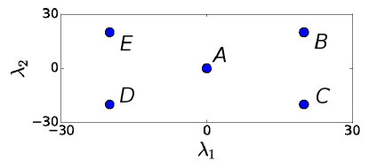
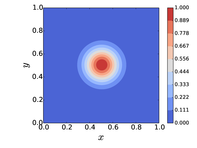
where denotes the LDO for the rotating shallow water dynamics (using and ) and represent perturbations in . In this section, the rotating shallow water equations represent the numerical model that we will learn via full-state regression, and represents the LDO corresponding to the dynamics that underlie our empirical dataset. The initial conditions used are displayed in Fig. 1.
We note that the 2-dimensional perturbation subspace (Eq. 21) we are using (referred to hence as ) is itself a subspace of the more general 18-dimensional energy-conserving subspace derived in §[4]: we are neglecting the 16 perturbation vectors associated with pure rotation and are only considering those which involve equal and opposite perturbations to kinetic and potential energies. We have chosen to further constrain the allowable LDO coefficient space in this way so as not to obfuscate the intended purpose of these examples. Our goal in these examples is simply to demonstrate LDO inference given different observables (e.g., full or partial state observables, coarse state observables) and different approaches to generating those observables (e.g., full LDO calculation or ROM approximation of the LDO). In principle, consideration of the full 18-dimensional space would change nothing about our inference methods; it would simply require more computational time and would be less easy to visualize.
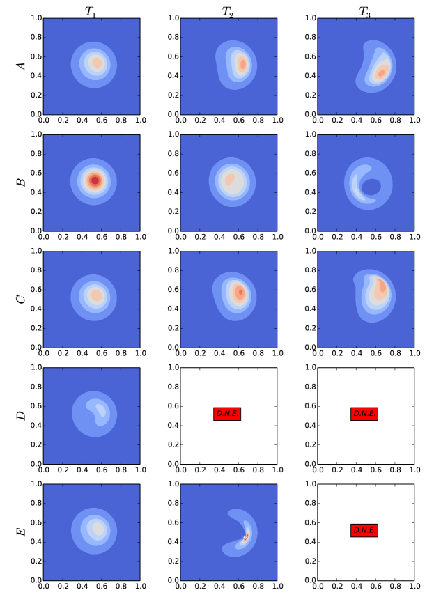
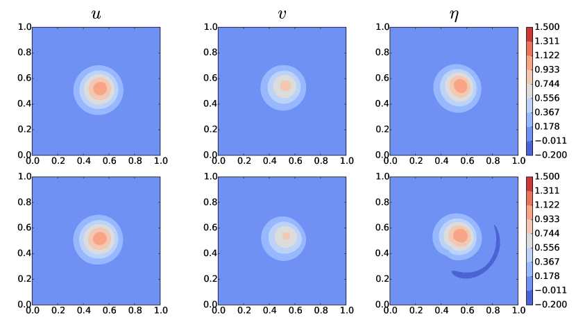
To illustrate the different dynamics possible in the subspace , we display snapshots of the state variable for the perturbed dynamics compared to those of the RSW equations in Fig. 2. As can be seen, the perturbed dynamics can look quite different relative to the base RSW dynamics after some time has passed. Also apparent from this is that the dynamics could potentially “blow-up” in finite-time, depending on the choice of LDO coefficient perturbations. We can get some insight into this by examination of the energy conservation statement Eq. 11, which reveals that there are terms present that are not perfect divergences and hence can act as sources/sinks for energy. The LDO perturbations we are allowing are chosen simply to be consistent with that differential energy law, which is obeyed by the RSW equations. Since that differential law does not guarantee that the total energy (i.e., integrated over space) will remain constant in time, we have no guarantee that the dynamics consistent with that law should exist for all time.

What follows are several demonstrations in which we attempt to infer the dynamics given different observables and different models for generating observables. Our first example is a simple demonstration of how the LDO may be regressed from data if one has access to the full state. After this, the remaining examples involve inferring the perturbed dynamics under the assumption of imperfect knowledge of the state and/or dynamics. In particular, we will investigate whether “coarse” (to be defined) state output is sufficient for inference purposes, and whether a POD-DEIM ROM identified for the RSW LDO can be used as a fast model for LDO inference.
6.1 Full-State Data Regression
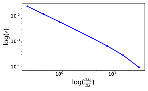
Our first example is a simple confirmation that a LDO may be regressed from data, as described in §[3.1]. Here, we use data generated from the RSW equations, with no perturbation to the dynamics. We generate data from the RSW equations using a structured Cartesian grid of 100100 spatial points. We use explicit timestepping with a time step . We perform a simple timestep convergence study in Fig. 3, in order to confirm that this value is within the asymptotic region of convergence. In this plot, corresponds to the time step value we have chosen to use. We forward integrate the RSW equations for a prescribed period of time for different values of the time step , and we calculate the L2-norm of the solution error between a solution obtained with that and the same solution calculated with high temporal resolution (corresponding to in the figure). Indeed, we observe that the L2-norm of the solution error decreases linearly on a log-log scale with a slope of approximately -1, which indicates algebraic solver convergence [36].
We begin by using least-squares regression with all quadratic combinations of the stencil elements as the basis . In all experiments, our stencil consists of the traditional 5-point stencil. For regression, we solve the normal equations:
| (22) |
As described previously, , , and . We use column-pivoted QR factorization to solve the problem in a well-conditioned way. Note that, in practice, we would begin by constraining the LDO parameter space with the prior physics knowledge that we introduced in §[4]. Indeed, we will solve the regression problem for this constrained case as well. However, first considering the unconstrained problem is a valuable pedagogical bridge that addresses several important issues in LDO regression that arise when there are many predictor variables.
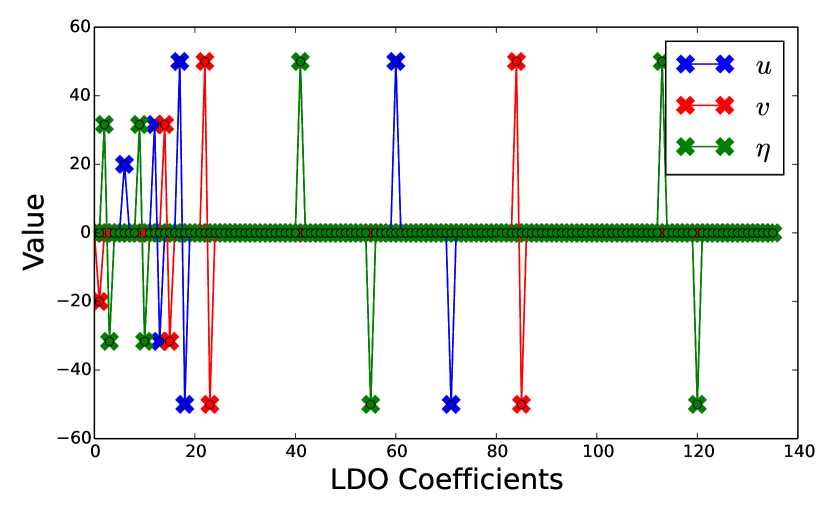
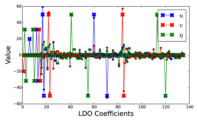
The main difficulty encountered when solving the unconstrained regression problem is that many of the predictors (i.e., the basis elements) are highly-correlated with one another (“multicollinearity”). This unfortunately makes the regression fairly non-robust. If the data are generated using Euler time-stepping, then the LDO should be able to exactly fit the data and in this special case, the results are fairly good (see Fig. 4(a)).
However, the results are much poorer if a different numerical scheme is used for time-stepping (e.g., Runge-Kutta). This is partially because the LDO can no longer fit the data exactly. For example, Runge-Kutta has the effect of both extending the stencil and enlarging the polynomial order of the LDO, which means that no LDO consisting of quadratic polynomial combinations of a five-point stencil will be able to exactly fit the data. This slight error is enough to greatly magnify the effects of the multicollinearity amongst the predictors, resulting in a relatively poorer datafit (see Fig. 4(b)). It should further be noted that in the example displayed in Fig. 4, five experiments with different initial conditions have been used in an attempt to factor out the “richness” of the dataset as a contributor to multicollinearity (indeed, if the dataset were to consist of only a single experiment, the predictors would be more highly correlated and the LDO coefficient fit would be even worse).
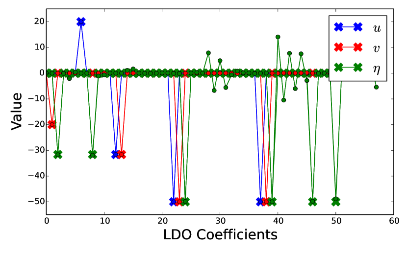
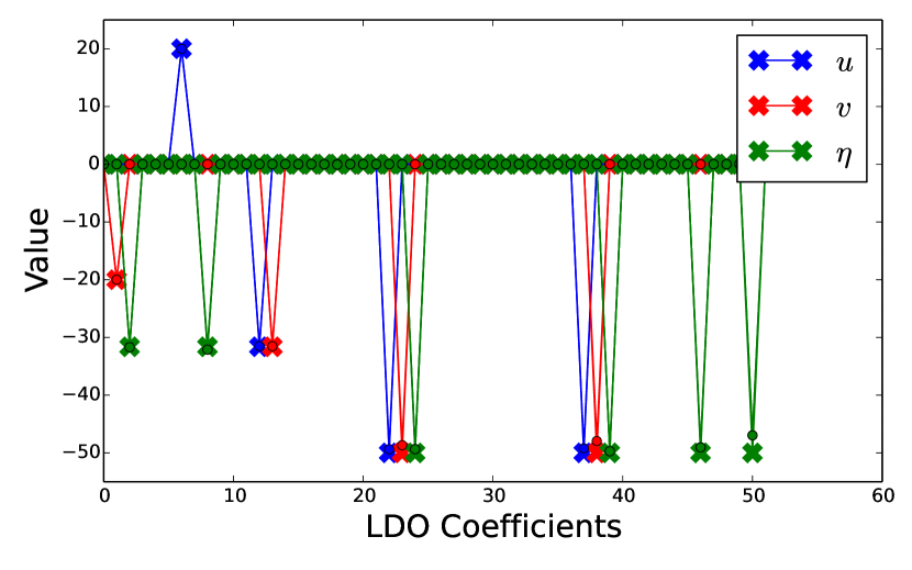
If we hypothesize that the main hurdle to achieving a robust numerical regression in our case is multicollinearity, then there are several “standard” strategies we may exploit to alleviate this issue. First, we can switch to using a basis consisting of only some differential operators (see Eq. 6); this illustrates another important reason for using such a basis in addition to LDO basis dimension reduction. Second, we can use the LASSO method instead of least-squares fitting. This method promotes a sparse solution to the LDO inference problem, which is justified on the hypothesis that the solution will be sparse. Note that, in practice, one would generally need to use a technique such as cross-validation to arrive at an acceptable weight parameter for LASSO. Fig. 5 shows an example of how using the differential operator basis – along with LASSO regression – can greatly improve the accuracy of the inferred LDO coefficients.
Ultimately, however, we are interested in solving the constrained regression problem, since that solution will inform the prior we use in the subsequent structural UQ step. The setup for this problem is a slight variation on what we have already done. As before, we solve the normal equations as in Eq. 22; however, the matrices we use are now as follows:
| (23) |
Here, the submatrices represent the components of the constrained basis vectors displayed in Eq. 21, and (the subscripts denote the respective state components). For a given snapshot of data, is calculated simply by applying the LDO corresponding to the RSW equations to that snapshot. Formulating the regression problem in this way, we calculate a numerical result of , which is very close to the true values of .
6.2 Single State Observable
We now turn our attention to the more difficult task of inferring the perturbed LDO given only imperfect knowledge of the state. This problem is meant to illustrate structural UQ – it is a scenario in which we only have access to incomplete information from an empirical dataset, and we wish to find a LDO that matches that QOI. The full-state inference of the RSW LDO in the previous section represents the numerical code model that we have learned, and now our goal is to search in an area of the energy-constrained subspace close to that numerical model for a LDO that produces a good match with the empirical QOI. Thus, the link between the previous step (regression) and this one (structural UQ) comes via the prior distribution we impose over the constrained LDO parameter space. Specifically, we choose a prior distribution that is centered at the mean values of that we inferred last section. Intuitively, our prior should weight points closer to that mean value more highly, and so we use a Gaussian distribution with a standard deviation of .
The incomplete QOI that we consider in this case will be the state variable , and nothing else. We assume that we are able to observe snapshots of this state variable at any point in time from the black-box dynamics of interest, and we wish to infer the LDO from this.
We elect to use the Metropolis MCMC algorithm to perform inference of the parameters . With access to the fully-resolved variable , we define our observable for the Metropolis algorithm as the RMS error of :
| (24) |
where is calculated from some LDO under consideration. We approximate the integral in Eq. 24 using 5,000 snapshots in time, collected using a time step , where denotes the grid point spacing (we use a 100100 grid of uniformly distributed points).
We define the Bayesian likelihood function as a normal distribution function of :
| (25) |
Of course, the parameter is a free-parameter that must be chosen; we set .
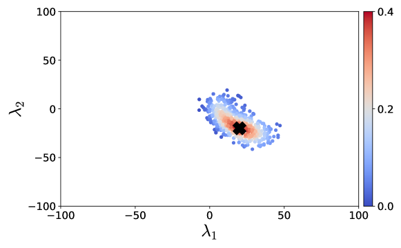
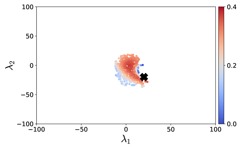
The posterior, estimated using 1,000 samples, is displayed in Fig. 6. We can clearly see that the MCMC samples converge strongly to a cluster which is exactly centered about the true values of .

6.3 Coarse-Data Observable
The previous examples illustrate how constrained inference may proceed in situations where access to one or more fully-resolved states is assumed. This is useful for demonstration purposes of the MCMC algorithm; however, the more realistic scenario for constrained inference occurs when we only have access to some observable function of the state which is of lower informational value. We show here an example of LDO inference in the energy-constrained subspace using state observations that are coarse in space and time. This emulates a situation in which only sparse observations of low spatial quality are available for structural UQ purposes.
In this example, we define “coarse” data by interpreting it as a kernel approximation to the actual state; for example,
| (26) |
is an approximation to the state . Different choices of the kernel are possible. For simplicity, we use the following discontinuous kernel:
| (27) |
where is a hypercube in space-time. This choice of kernel corresponds to a local space-time average in some . Thus, we can then coarsen the data by dividing space-time into several non-overlapping boxes, and then computing the local average within each of these boxes via Eq. 26. If we take this locally-averaged data to be our observable, we may define an error metric just as in Eq. 24, except with and replaced by their coarsened versions. One way to express the level of coarsening is with the ratio of the fine-to-coarse grid size. In this example, we use a spatial coarsening ratio of 25 (i.e., 25 fine grid points are contained in each coarse grid box), and a temporal coarsening ratio of 25 (i.e., 25 snapshots in time are averaged together in the coarsening operation). Example snapshots using this process are shown in Fig. 7.
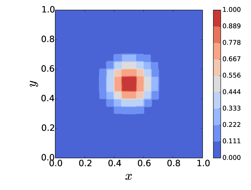
As in the previous example, we perform our inference in the energy-constrained subspace , and we are attempting to infer the parameters . The MCMC posterior (calculated with 1,000 samples, and in Eq. 25) using the coarse-data observable is shown in Fig. 8. The MCMC samples converge as before to a cluster in parameter space, which is roughly centered about the true values.
6.4 Coarse-Data Observable, Computed with a ROM
In this example, we investigate whether LDO coefficient inference can be successfully done using a ROM identified for the base LDO in place of the actual LDO corresponding to a given perturbation. The methodology for calculating a LDO ROM is sketched in §[5]. Again, the motivation for this is computational expense: doing Bayesian inference in LDO space could be expensive, even with energy constraints, simply because it involves calculating discrete-time dynamics by forward-integrating candidate LDOs.
As before, our base LDO (and the ROM identified for it) corresponds to the RSW equations (which corresponds to ). We use the same energy-preserving perturbation to the base LDO as in the previous example, and perform our inference in the corresponding 2-dimensional space . We take our observable to be the state variable , coarsened with the operator as defined in Eq. 26. We use the error metric in Eq. 24 (albeit with the coarsened versions of ).
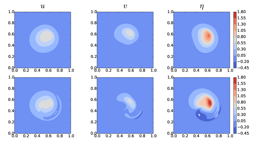
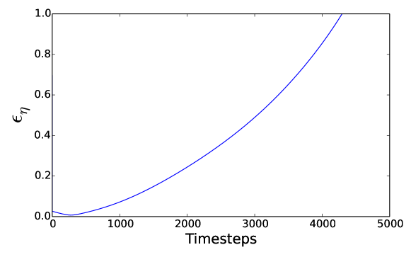
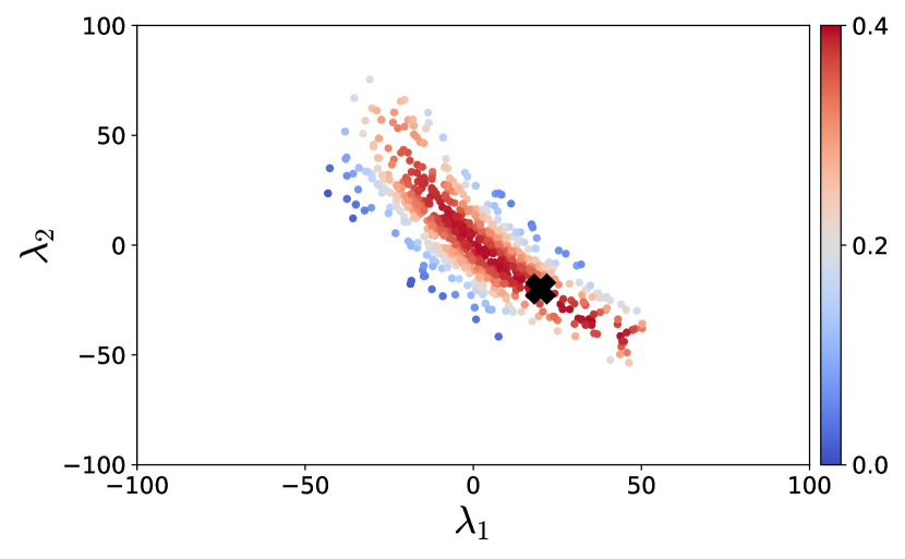
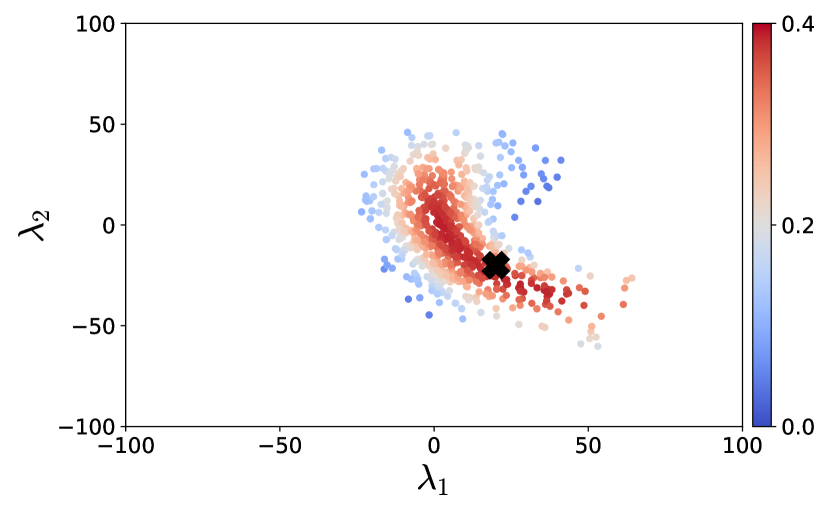
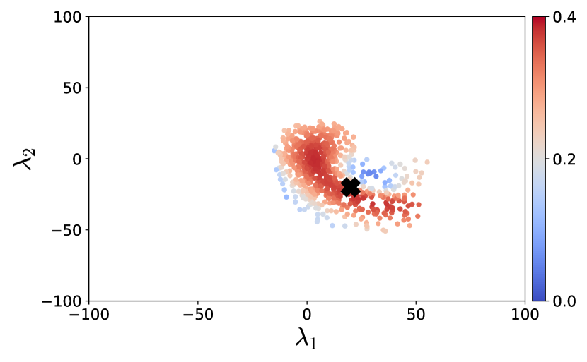
To begin, we might wonder about collecting increasing numbers of snapshots from candidate LDO simulations in the MCMC algorithm, and how this affects the accuracy and precision of the calculated posterior. Usually, we would expect this relationship to be monotonic: more data is always better. However, because we are using a ROM whose accuracy is limited by the original base data used to derive it (i.e., snapshots from the RSW LDO), this is not necessarily the case. That is, there is a temporal trade-off between aggregating more information and the degrading accuracy of the ROM. Since all simulations begin with the same initial conditions as those used to derive the RSW ROM (shown in Fig. 1), the ROM is most accurate for a given perturbed LDO at early times, when the spatial characteristics of the state variables are close to those of the RSW equations and hence largely spanned by the POD bases used to describe them in the ROM (see Fig. 9(a)). However, as time progresses, the spatial patterns of the solutions quickly diverge from those exhibited by the RSW equations as the differences in structural governing dynamics become increasingly apparent. While this information is useful in discriminating amongst different LDOs, it is only useful if the ROM can reproduce it. As would be expected, the accuracy of the ROM does degrade as the spatial patterns exhibited by a given LDO diverge from those used by the ROM to describe them (see Fig. 9(a), 9(b) and 10).
Thus, we are led to conclude that the best compromise available to us is a middle ground in which we collect just enough observable data from the ROM in the MCMC algorithm such that the relevant structural differences begin to manifest themselves, but not so much that the growing inaccuracies of the ROM incorrectly skew our inference results. Fig. 11 provides some empirical evidence of this. We see that if we limit ourselves to a relatively low number of snapshots (Fig. 11(a)) for inference purposes, then the highest likelihood samples in our posterior lie along a broad swath in parameter space. On the other hand, using a relatively high number of snapshots (Fig. 11(d)) collapses the ridge, but the posterior now completely misses the true parameters. A number of snapshots between these two extremes (Fig. 11(b) or 11(c)) produces a reasonable compromise between accuracy and precision.
We should also briefly discuss a procedure for determining the temporal threshold at which we stop collecting data due to the decreasing fidelity of the ROM. The most straightforward way to do this is to simply choose some random samples in LDO parameter space, do a forward simulation of the corresponding full LDO without a ROM, and then redo those calculations using the ROM. One could then compare the ROM-calculated solutions against the full LDO simulations and get an estimate of the length of time over which the ROM is able to provide reasonably faithful predictions. Certainly, this approach does add some computational overhead, and depending on the computational expense of the full LDO system, the user might be limited in terms of how many full candidate LDO simulations they can afford to do. Notwithstanding, this is a simple and accurate way of estimating the ROM’s fidelity over the relevant parameter space. We would recommend doing this in practice.
Additionally, we should add that there are statistical tools for explicitly integrating terms that attempt to account for model error into computer simulations (see, for example, [37, 38]). If we wanted to go a step further with the ROM-error accounting/correction, then it is possible that these tools could be useful. One could potentially introduce a discrepancy term that would account for the ROM error. Of course, we would have to have some prior knowledge about the ROM error in order to do this accurately, which we might obtain by the process outlined above.
Although we have lost some of the statistical precision in the posterior by using a ROM for the LDO, we have gained a significant advantage in terms of computational runtime. One way to assess this is the number of floating point operations required to calculate a LDO versus a POD-DEIM ROM. For the former, one must first compute the terms in the basis matrix at each spatial point, which is a total of operations (where denotes the number of grid points). Next, one must compute the matrix product , which requires operations, giving operations. In our examples, , , , , so flops are required (for each timestep). By comparison, the ROM first involves computing the POD state approximate at the DEIM points and at all of the points in their respective stencils (a total of at most points), which involves operations (where is the number of state POD modes). Next, the LDO must be evaluated on those DEIM points, which amounts to calculating the basis elements and then computing on each of those points, which involves operations. Finally, the matrix product must be computed, which involves operations. Altogether, the total number of operations for each timestep is . In our examples, we use and , giving a total of operations. This is around 100 times fewer flops and represents a significant computational alleviation. Empirically, we find that the ROM-based simulation is approximately 25 times faster than the full LDO simulation, which is reasonably close to our asymptotic operation-count analysis.
6.5 Other Issues: Multiple Time Scales, State Space Location of Data
In this section, we briefly address some questions related to the effect of the underlying dynamics – and the numerical code that implements those dynamics – on the accuracy of the inferred LDO. Specifically, we consider how LDO accuracy is affected by dynamics with fast/slow time scales, and how it is affected by the location of the data in state space. This is motivated by a dynamical systems perspective: there could be regions of state space in which some terms in the governing dynamics are relatively small in magnitude (e.g., close to a fixed point where linear dynamics dominate), which might present a problem to the regression method that attempts to infer them. The practical concern this presents is that in order to accurately learn those terms, it may be necessary to sample the dynamics at many timescales and many locations in state space – which could be expensive – in order to infer a reasonable LDO.
We also note that in these examples, we use a set of features that does not correspond exactly to the operators used in the discretization of the numerical solver. This is important in the sense that we would like for our feature set to be both agnostic to and independent of the discretization used in the actual numerical solver – if this were not the case, then we would always have to use a feature set that included an exact replication of all the algorithms implemented in the numerical code, which is neither desirable (nor feasible, often) from the standpoint of system identification.
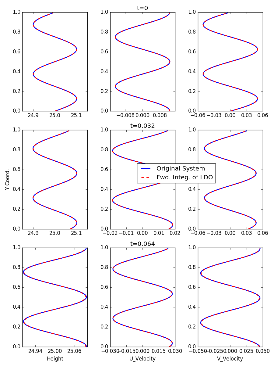
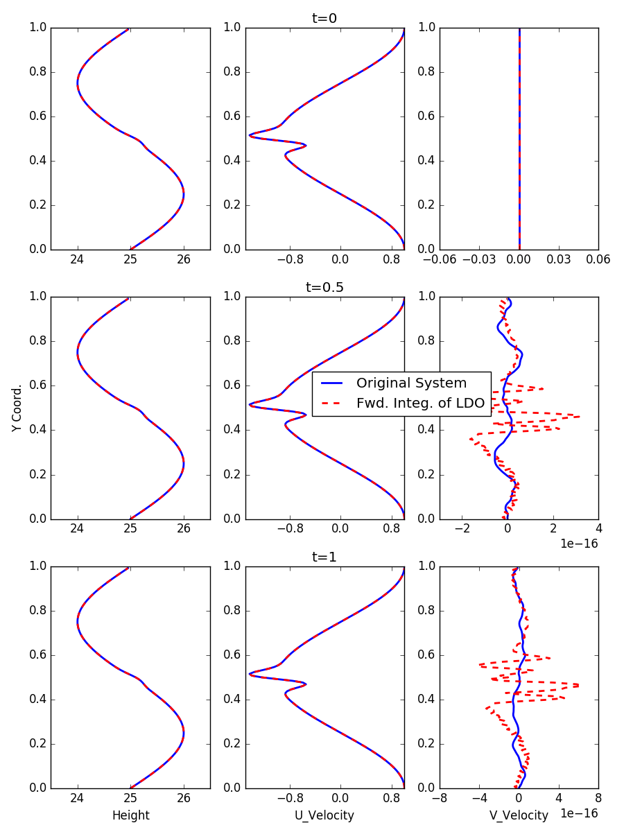
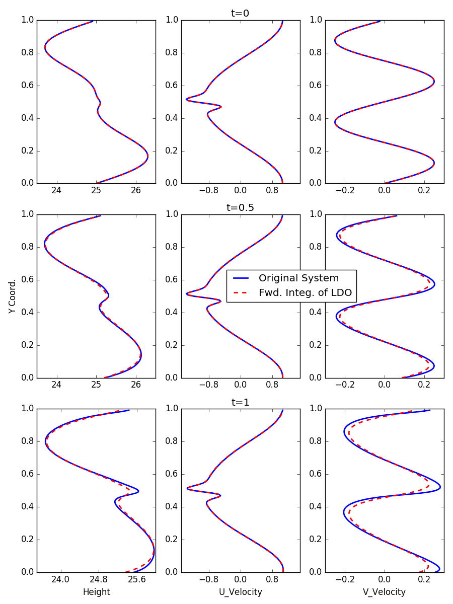
A nice property of the RSW equations is that they allow for the two fundamental classes of fluid motion found in oceanic dynamics: slow vortical motions and fast (inertia-gravity) wave motions. Thus, they provide a nice testbed for us to investigate the effects of multiple time scales and the location of the data in state space on LDO accuracy. To do that, we assess the accuracy of the inferred LDO in three separate cases. In the first case, the data used for the LDO inference is a trajectory along the fast mode of the linearized system. In the second case, the data used is drawn from a trajectory along the slow linear mode, while the third case is a more general trajectory that includes both fast and slow components.
Fig. 12 shows a comparison of the evolution of the state of the system as obtained by the forward-integration of the inferred LDO against the evolution in the original system for a fast mode initial condition. We note that the LDO inference used data from the original solver only up to a time of 0.03 so that the snapshots shown at times 0.032 and 0.064 are both extrapolations from the point of view of LDO inference. The comparison is seen to be good. Thus, we see that in order to learn the fast linear dynamics, we need not worry about collecting data for long periods of time or in multiple regimes of state space.
As mentioned earlier, we would also like to confirm in these examples that the LDO inference procedure does not demand that the features used be exact replicas of those operators implemented in the numerical solver. Thus, the data used for the LDO inference come from a pseudo-spectral solver, while the actual features themselves are consistent with the formulation of §[2]. In light of the results in Fig. 12, we see that for the fast mode dynamics, it is indeed possible to infer a reasonable LDO using features that are independent from the operators implemented in the numerical solver.
We now consider the evolution of a slow-mode initial condition. Fig. 13 shows a similar comparison as in the fast-mode initial condition case previously discussed. In this case, the LDO inference used data from the original solver only up to a time of 0.01 so that the snapshots shown at times 0.5 and 1.0 are both (long-term) extrapolations from the point of view of LDO inference. Again, the comparison is seen to be good, indicating that – as in the previous case – it is not necessary to exhaustively sample wide swaths of state space for long time periods, or to use a set of features that correspond exactly to the operators used in the numerical solver.
Finally, we consider the evolution of an initial condition that represents a combination of both fast and slow mode components, as occurs in the oceans and the atmosphere. In this example, the u-component of velocity and the height fields contain both the slow vortical components and the fast wave components whereas the v-component of velocity contains only the fast wave component. This case represents a qualitatively important difference from the previous two, since our initial condition no longer lies along an eigenvector of the linearized system, and so nonlinear terms may be more pronounced for this case. Fig. 14 displays a comparison of the evolution of the state of the system as obtained by the forward-integration of the inferred LDO against the evolution in the original system. In this example, data up to a time of 0.75 was used in inferring the LDO, thus making the snapshots at a time of 1.00 LDO-extrapolations. In contrast to the previous cases, the LDO evolution here is seen to be only approximately correct.
One possible explanation for these discrepancies is that there is some error in the inferred nonlinear terms of the LDO, which was effectively irrelevant in the previous two cases where linear dynamics dominated. This could be the case, for example, if the features we have used can only at best provide a cruder approximation of the dynamics relative to the more accurate psuedo-spectral solver implementation. Another possibility is that the flow evolution is highly sensitive to location in state space, and so even slight differences between the two systems compound quickly in time. This could be the case if, for example, the underlying flow dynamics were chaotic in this regime of state space. While the former explanation is an artifact of the inference procedure, the latter is a fundamental property of the dynamics, and it is not immediately clear which of the two (or both) accounts for the observed discrepancies. Regardless, in order to not detract from the main narrative of the article, we postpone a discussion of such issues and attendant modifications to the LDO inference procedures to a future article.
7 Conclusions
The intended purpose of this paper was to (1) define a mathematical representation of a model structure that can be manipulated easily and independently of the original numerical source code, (2) infer this structure non-intrusively using simulation output, (3) efficiently approximate the impact of perturbations to a model structure on the model dynamics, using ROM techniques, and (4) sample the space of structural uncertainties consistent with data/physical constraints, and propagate these to uncertainties in predictions (Bayesian calibration).
The testbed problem on which we demonstrated these objectives was the 2D rotating shallow water equations. We successfully inferred LDO approximations to the RSW continuum dynamics using two different sets of features defined on the stencil field values (i.e., quadratic polynomials and differential operator approximations). We then saw how it helped to introduce some assumptions about allowable LDO structures, using energy conservation laws and sparsity-promoting regression. We constructed a ROM for the purpose of efficient Bayesian calibration, using non-intrusive system identification (POD-DEIM-Galerkin projection). We found that the predictive accuracy POD-DEIM-Galerkin model decreases monotonically with time; this was expected, since in the Bayesian calibration we are changing the dynamics from which the ROM was derived. However, we also found some evidence that the ROM can be sufficiently accurate for an initial period of time such that we can “rule out” large areas of LDO parameter space before it degrades too much. Using this ROM, we were able to efficiently generate and search many hypothetical model structures in LDO parameter space and infer those which were consistent with a coarse observable quantity of interest.
The envisioned practical setting for these ideas is quantification/learning of subgrid physics. Our intent is to build a dictionary of local features that is capable of representing a suite of subgrid models, learn several such numerical closure models in that basis, and then search around that area of feature space for a LDO that reproduces a QOI from some dataset that we regard as the “truth”.
As we have demonstrated the basics on a toy problem (i.e., the shallow water equations), the next step is to apply these ideas to more complex numerical codes. We are currently attempting to do this with MPAS-Ocean [39], which is an unstructured code for ocean dynamics that has several horizontal/vertical mixing parameterizations and closures implemented. We hope to learn these closure models in a local feature space, and then use the results to guide an inference of the subgrid physics for an emprical dataset. This broad topic will be the subject of future follow-up studies on our part.
8 Acknowledgments
Los Alamos Report LA-UR-18-21957. Funded by the Department of Energy at Los Alamos National Laboratory under contract DE-AC52-06NA25396.
References
- [1] Solomon, S., Qin, D., Manning, M., Averyt, K., and Marquis, M., Climate change 2007-the physical science basis: Working group I contribution to the fourth assessment report of the IPCC, Vol. 4, Cambridge university press, 2007.
- [2] Tebaldi, C., Smith, R.L., Nychka, D., and Mearns, L.O., Quantifying uncertainty in projections of regional climate change: A bayesian approach to the analysis of multimodel ensembles, Journal of Climate, 18(10):1524–1540, 2005.
- [3] Krishnamurti, T.N., Kishtawal, C., Zhang, Z., LaRow, T., Bachiochi, D., Williford, E., Gadgil, S., and Surendran, S., Multimodel ensemble forecasts for weather and seasonal climate, Journal of Climate, 13(23):4196–4216, 2000.
- [4] Lumley, J.L., The structure of inhomogeneous turbulent flows, In: Yaglom, A.M. and Tartarski, V.R. (Eds.), Atmospheric Turbulence and Radio Wave Propagation, pp. 166–178, 1967.
- [5] Holmes, P., Lumley, J.L., Berkooz, G., and Rowley, C.W., Turbulence, coherent structures, dynamical systems and symmetry, Cambridge University Press, 2nd edition, 2012.
- [6] Sirovich, L., Turbulence and the dynamics of coherent structures, Quarterly of Applied Mathematics, XLV(3):561–582, 1987.
- [7] Berkooz, G., Holmes, P., and Lumley, J.L., The proper orthogonal decomposition in the analysis of turbulent flows, Ann. Rev. Fluid Mech., 25:539–575, 1993.
- [8] Rowley, C.W., Mezic, I., Bagheri, S., Schlatter, P., and Henningson, D., Spectral analysis of nonlinear flows, Journal of Fluid Mechanics, 641:115–127, 2009.
- [9] Schmid, P., Dynamic mode decomposition of numerical and experimental data, In Bull. Amer. Phys. Soc., 61st APS meeting, American Physical Society, p. 208, 2008.
- [10] J. H. Tu and C. W. Rowley and D. M. Luchtenburg and S. L. Brunton and J. N. Kutz, On dynamic mode decomposition: theory and applications, Journal of Computational Dynamics, 1(2):391–421, 2014.
- [11] Williams, M.O., Kevrekidis, I.G., and Rowley, C.W., A data–driven approximation of the koopman operator: Extending dynamic mode decomposition, Journal of Nonlinear Science, 25(6):1307–1346, 2015.
- [12] Williams, M.O., Rowley, C.W., and Kevrekidis, I.G., A kernel-based method for data-driven koopman spectral analysis, Journal of Computational Dynamics, 2(2):247–265, 2015.
- [13] Hemati, M.S., Williams, M.O., and Rowley, C.W., Dynamic mode decomposition for large and streaming datasets, Physics of Fluids, 26, 2014.
- [14] Proctor, J.L., Brunton, S.L., and Kutz, J.N., Dynamic mode decomposition with control, SIAM Journal on Applied Dynamical Systems, 15(1):142–161, 2016.
- [15] Loiseau, J.C. and Brunton, S.L., Constrained sparse galerkin regression, Journal of Fluid Mechanics, 838:42–67, 2018.
- [16] Brunton, S.L., Proctor, J.L., and Kutz, J.N., Discovering governing equations from data by sparse identification of nonlinear dynamical systems, Proceedings of the National Academy of Sciences, p. 201517384, 2016.
- [17] Rudy, S.H., Brunton, S.L., Proctor, J.L., and Kutz, J.N., Data-driven discovery of partial differential equations, Science Advances, 3(4), 2017.
- [18] Peherstorfer, B. and Willcox, K., Data-driven operator inference for nonintrusive projection-based model reduction, Computer Methods in Applied Mechanics and Engineering, 306:196–215, 2016.
- [19] Peherstorfer, B. and Willcox, K., Dynamic data-driven reduced-order models, Computer Methods in Applied Mechanics and Engineering, 291(0):21–41, 2015.
- [20] Quade, M., Abel, M., Shafi, K., and Niven, R., Prediction of dynamical systems by symbolic regression, Physical Review E, 94(1), 2016.
- [21] Sirignano, J. and Spiliopoulos, K. DGM: a deep learning algorithm for solving partial differential equations. arXiv:1708.07469, 2017.
- [22] Chen, H., Blackbox stencil interpolation method for model reduction, PhD thesis, Massachusetts Institute of Technology, 2012.
- [23] Metropolis, N., Rosenbluth, A.W., Rosenbluth, M.N., and Teller, A.H., Equations of state calculations by fast computing machines, Journal of Chemical Physics, 21(6):1087–1092, 1953.
- [24] Hastings, W.K., Monte carlo sampling methods using markov chains and their applications, Biometrika, 57(1):97–109, 1970.
- [25] Majda, A.J. and Embid, P., Averaging over fast gravity waves for geophysical flows with unbalanced initial data, Theoretical and Computational Fluid Dynamics, 11:155–169, 1998.
- [26] Majda, A.J., Introduction to PDEs and waves for the atmosphere and ocean, American Mathematical Society, 2003.
- [27] An, S.S., Kim, T., and James, D.L., Optimizing cubature for efficient integration of subspace deformations, ACM transactions on graphics (TOG), 27(5):165, 2008.
- [28] Carlberg, K., Choi, Y., and Sargsyan, S., Conservative model reduction for finite-volume models, Journal of Computational Physics, 371:280–314, 2018.
- [29] Carlberg, K., Tuminaro, R., and Boggs, P., Preserving lagrangian structure in nonlinear model reduction with application to structural dynamics, SIAM Journal on Scientific Computing, 37(2):B153–B184, 2015.
- [30] Farhat, C., Avery, P., Chapman, T., and Cortial, J., Dimensional reduction of nonlinear finite element dynamic models with finite rotations and energy-based mesh sampling and weighting for computational efficiency, International Journal for Numerical Methods in Engineering, 98(9):625–662, 2014.
- [31] Farhat, C., Chapman, T., and Avery, P., Structure-preserving, stability, and accuracy properties of the energy-conserving sampling and weighting method for the hyper reduction of nonlinear finite element dynamic models, International Journal for Numerical Methods in Engineering, 102(5):1077–1110, 2015.
- [32] Karasözen, B. and Uzunca, M., Energy preserving model order reduction of the nonlinear schrödinger equation, Advances in Computational Mathematics, pp. 1–28, 2017.
- [33] Lall, S., Krysl, P., and Marsden, J.E., Structure-preserving model reduction for mechanical systems, Physica D: Nonlinear Phenomena, 184(1-4):304–318, 2003.
- [34] Barrault, M., Maday, Y., Nguyen, N.C., and Patera, A.T., An ‘empirical interpolation’ method: application to efficient reduced-basis discretization of partial differential equations, Comptes Rendus Mathematique, 339(9):667–672, 2004.
- [35] Chaturantabut, S. and Sorensen, D.C., Nonlinear model reduction via discrete empirical interpolation, SIAM Journal of Scientific Computing, 32(5):2737–2764, 2010.
- [36] Wang, Z., High-order methods for the euler and navier–stokes equations on unstructured grids, Progress in Aerospace Sciences, 43(1-3):1–41, 2007.
- [37] Kennedy, M.C., O’Hagan, A., and Higgins, N. Bayesian analysis of computer code outputs. In Quantitative methods for current environmental issues, pp. 227–243. Springer, 2002.
- [38] Brynjarsdóttir, J. and O’Hagan, A., Learning about physical parameters: The importance of model discrepancy, Inverse Problems, 30(11):114007, 2014.
- [39] Ringler, T., Petersen, M., Higdon, R.L., Jacobsen, D., Jones, P.W., and Maltrud, M., A multi-resolution approach to global ocean modeling, Ocean Modelling, 69:211 – 232, 2013.