Contour Parametrization via Anisotropic Mean Curvature Flows
Abstract.
We present a new implementation of anisotropic mean curvature flow for contour recognition. Our procedure couples the mean curvature flow of planar closed smooth curves, with an external field from a potential of point-wise charges. This coupling constrains the motion when the curve matches a picture placed as background. We include a stability criteria for our numerical approximation.
Introduction
Many applied and theoretical problems have been studied through the analysis of manifold deformations [5, 6, 10]. The description of these deformations by an evolution equation imposed via a geometric quantity are referred to as geometric flows. Applications include, for example, the growth of crystals, the modeling of fluids, and digital image recognition. Since their conception there has been continued interest in the development of numerical approximations to these flows [21].
The difficulty in analyzing these flows numerically depends on the geometric quantity in evolution (e.g. curvature, metric tensor, the manifold itself). In particular, the mean curvature flow (MCF) deforms a hypersurface in the normal direction with a speed proportional to its mean curvature . This flow has an associated quasilinear parabolic equation in terms of an immersion of the hypersurface into the ambient manifold:
| (1) |
The numerical methods employed to solve this equation are classified as Eulerian or Lagrangian methods, depending on the discrete representation of the surface or curve in evolution. In Eulerian methods the evolution is tracked by values at fixed positions on a gridded ambient. Conversely, in Lagrangian methods, the object in evolution is tracked explicitly through the position of its points. In consequence, Lagrangian methods have two advantages: they require smaller data storage than Eulerian methods, and the solution is computed explicitly; although generally their error estimates are difficult to estimate precisely. Eulerian methods are now a powerful and frequently used technique for mean curvature flow applications since the development of the Level Set Method [21, 24]. To our knowledge, there are very few examples of Lagrangian methods that approach this problem [25, 13], our work adds to this list.
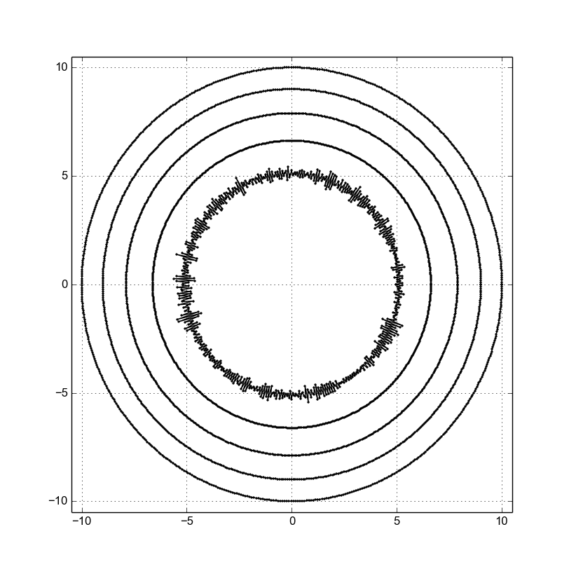
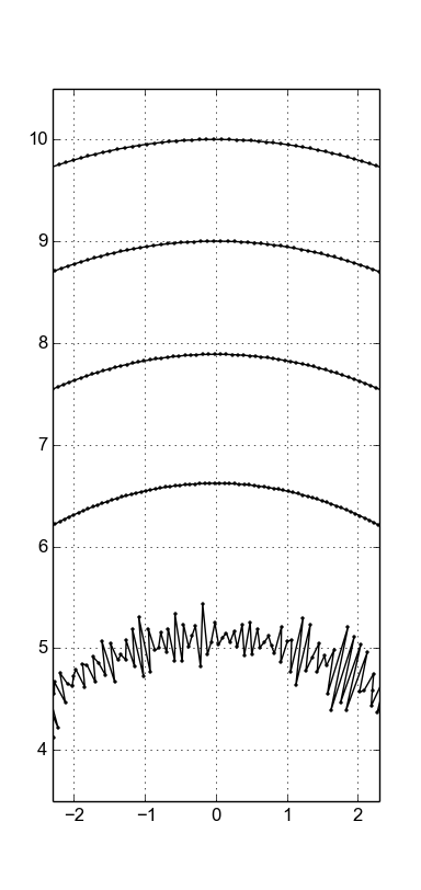
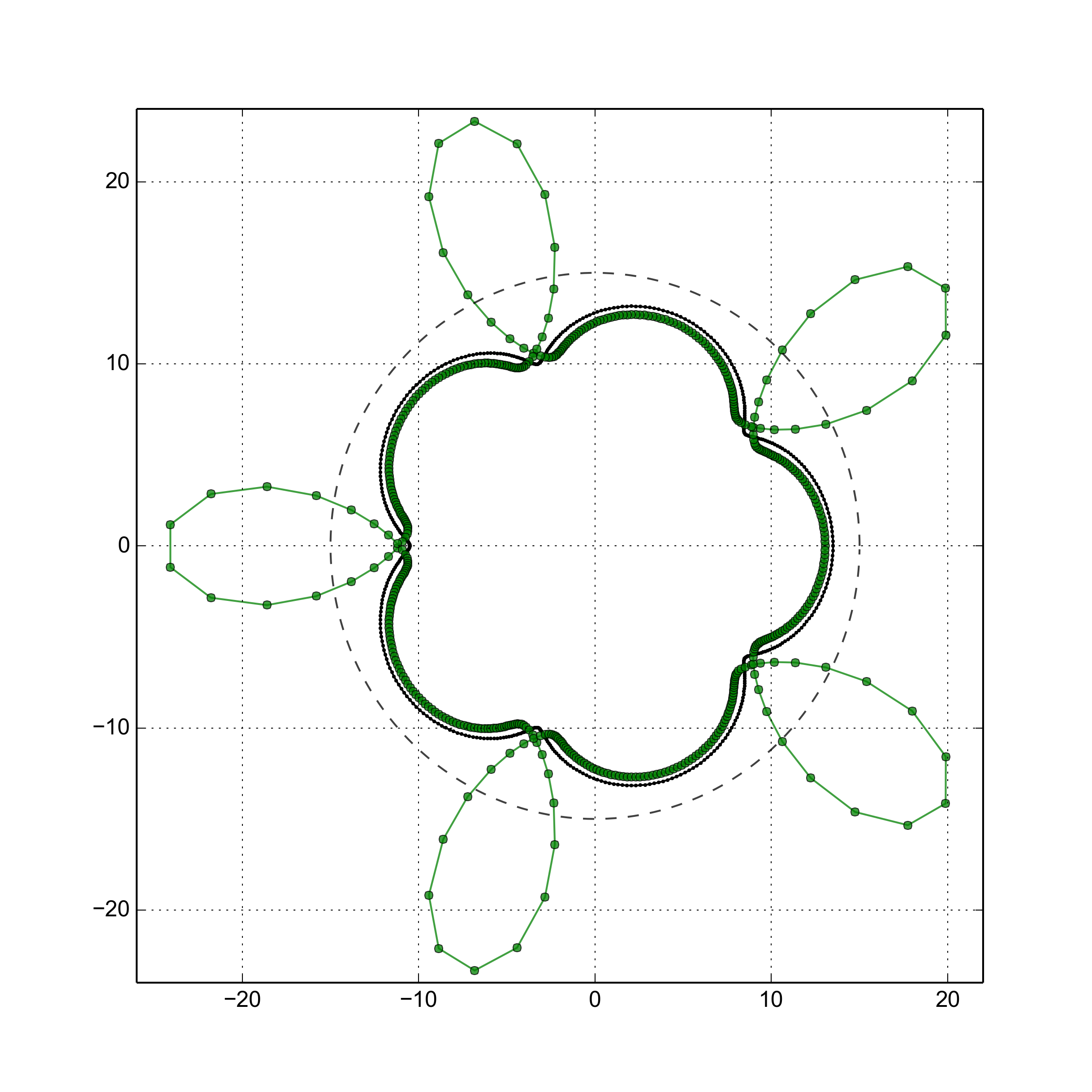
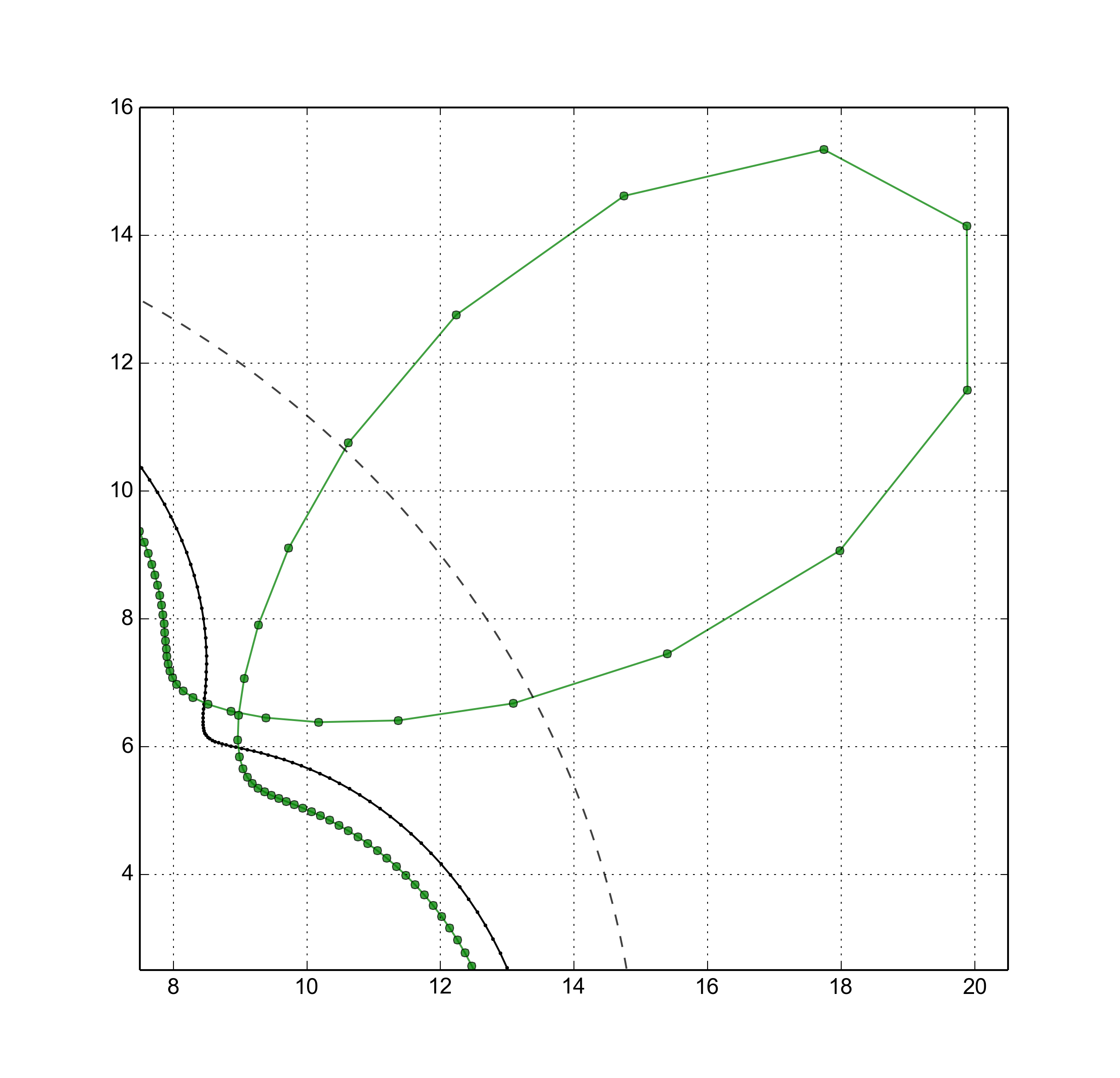
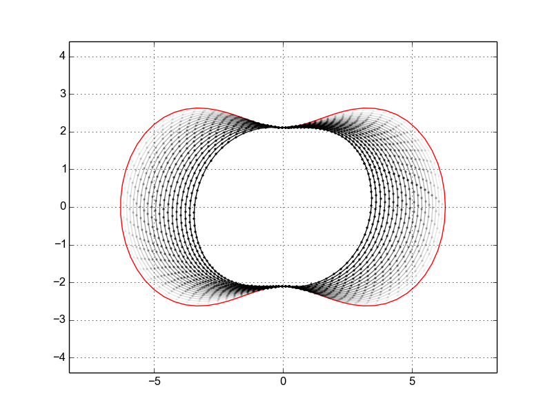
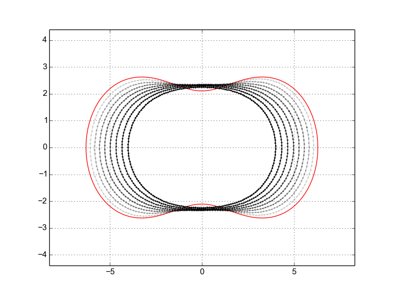
The disadvantage of Lagrangian methods are discussed in many works. Two problems arise commonly when straightforward discretization of equation ( 1) is performed: (i) a numerical instability as shown in Figure 1 and (ii) loop formation which contradicts the comparison principle (see [7, 18]), as shown in Figure 2 for a cycloid (solid line) and its first iteration result (polygonal curve) compared with a circumference (dashed curve).
Here we present a Lagrangian method for contour parametrization. To accomplish this application, we assume that a planar closed and differentiable curve is drawn on a 2D digital image. Then, we evolve the curve by mean curvature flow, but constraining the motion of the curve by the objects in the image. If only one object is initially inside the curve, as the curve shrinks, it will match parts of the boundary of the object. The main problem using MCF to recognize images is to couple the restriction and the flow, because it implies that the curve is not evolving uniformly. That is, not all points in the curve will move, even when the curvature at those points is different from zero. This kind of flow is called anisotropic. To avoid certain numerical difficulties, our scheme considers a curve motion along tangential and normal directions, as in [13]. The results of [13] correspond to an unconstrained flow, so the stability and convergence results found there can not be compared with ours. Since the numerical procedure is based on certain MCF properties, we provide the necessary technical details about existence and uniqueness of solutions for MCF in Theorems 4 and 9.
Kimura developed a Lagrangian method which numerically reproduces the mean curvature flow for curves, based on a redistribution of points by reparametrization by arc length [13]. That method represents an initial simply closed smooth curve by an ordered set of points. The position of each point is updated to represent the curve after a time . This method assumes a tubular neighborhood in which, for a small time interval , the whole evolution is inside, and therefore may be parameterized as
In this tubular neighborhood the map , given by
is invertible. A correction term is then added to Euler’s formula (see [13]). Figures (3- 5) show numerical examples with Kimura’s method, the evolution in time is represented by the z axis.
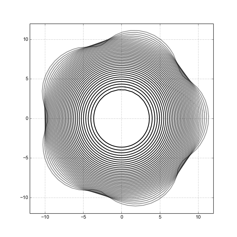
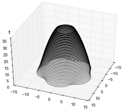
(a) (b)
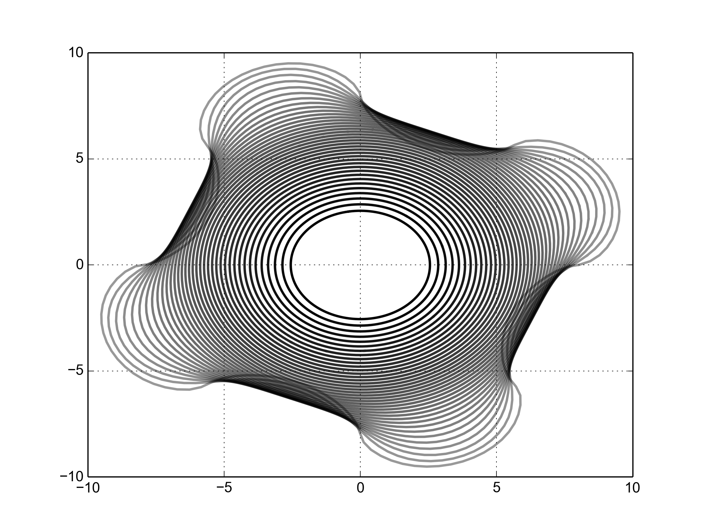
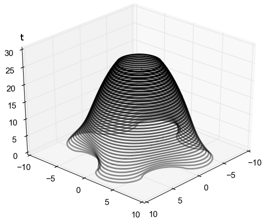
(a) (b)
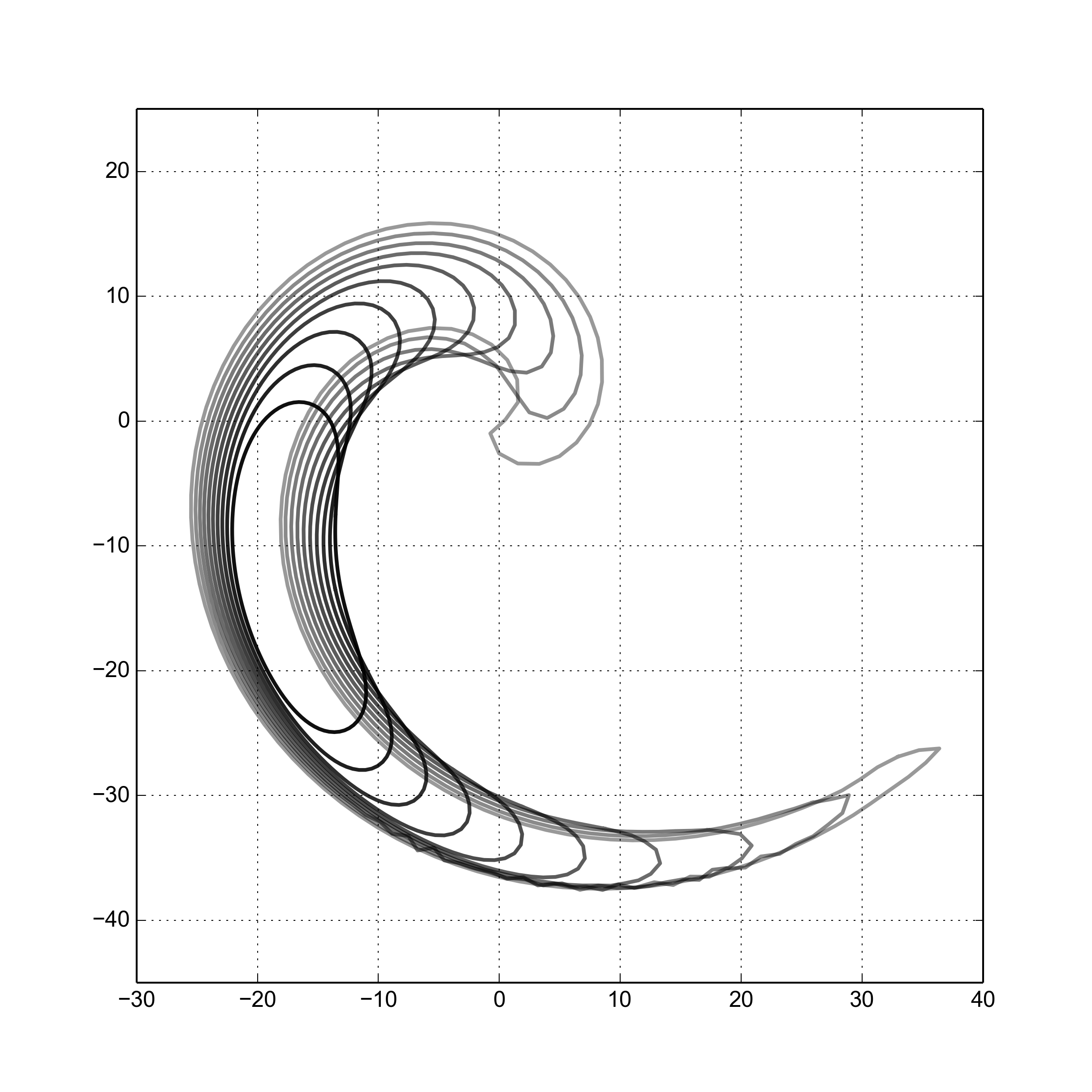
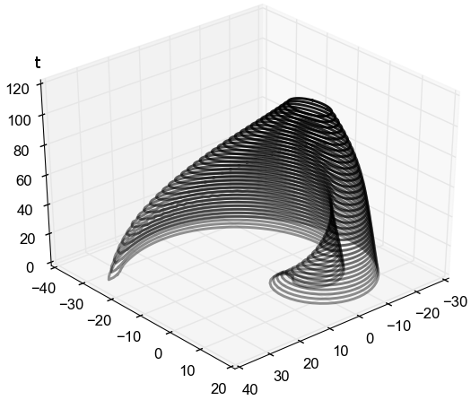
(a) (b)
Our main theoretical result is the postulation of an anisotropic MCF, for which short time existence of solutions is shown in Theorem (10). Furthermore, we detail a numerical scheme to approximate solutions and apply it to the task of contour parametrization.
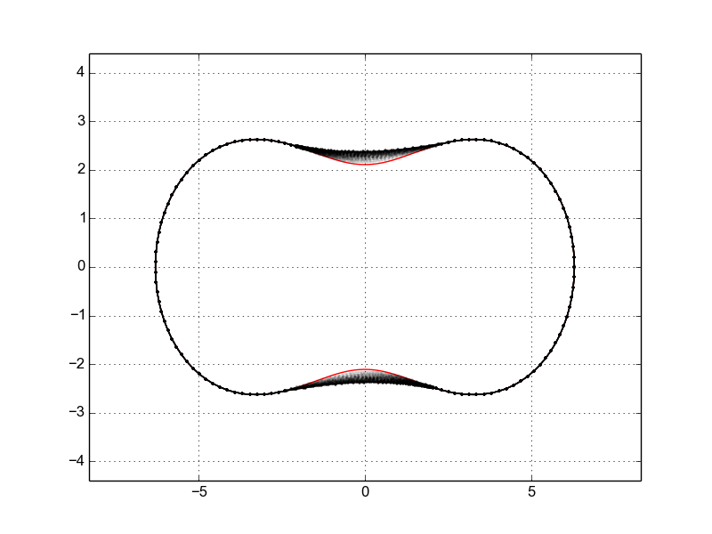
Many varieties of an anisotropic MCF can be proposed, Figure (7) compares the MCF with two versions of anisotropic MCF. Our evolution scheme is an adaptation for contour recognition of Kimura’s planar curve evolution. We approach the stability of our scheme through von Neumann’s analysis. In our analysis, the parameters in error propagators (see Equation (38)) are time dependent. Then, the stability condition cannot be determined for all time but only for the next time step. We establish our main stability criterion in Proposition 13.
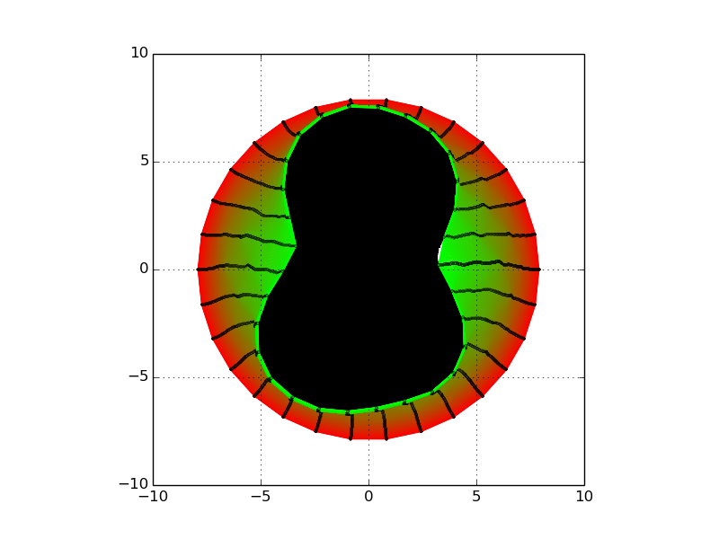
In contrast to previous approaches, our method is a Lagrangian scheme whose main features are: (I) Estimation of curvature bounds are not required. (II) It is formulated as a Poisson problem with a boundary condition given implicitly. This condition links Poisson’s problem with the MCF. Our proposed Poisson problem couples MCF and the field due to a point charge distribution. (III) Finding a solution requires to solve a linear system. (IV) When it is implemented to a contour parametrization problem, only the pixel value at each point constraints the motion. (V) These constraints are handled through the source function and the boundary condition in Poisson’s equation. Our numerical experiments reveal that this Poisson formulation can match some non-convex shapes perfectly. In general, matching non-convex shapes successfully depends on the charge distribution. Our scheme takes the numerical approximation for curvature and an equidistant distribution of points from [13], and through our proposed Poisson formulation we can handle these constraints. In Figure 6, we present a contour matching with an initial circumference as the evolving curve. The color gradient advances with time from red to green. A high contrast between red and green represents a fast matching, and a smooth color gradient indicates regions which require more iterations to reach the shape boundary in black.
Outline
This work is presented as follows: §1 the proof of existence and uniqueness of solutions for MCF and some of its properties, included for completeness sake; §2 the presentation of our conditioned or anisotropic MCF and formulas for its solutions; §3 the numerical implementation of our anisotropic flow; §4 the implementation of the anisotropic MCF for contour parametrization; §5 details the stability properties of our numerical scheme, and §6 contains our conclusions and suggestions for future directions.
1. Short-time Existence and Uniqueness of Solutions
The main result of this section proves existence and uniqueness of solutions to an isotropic version of MCF. The proof includes new technical details, in particular bounds on the displacement of the immersed curve (equation (4) in Lemma 3), which are essential for the computations in the associated numerical problem in section 3.
This proof requires to rewrite equation (1) in terms of a reparametrization of the evolving manifold. Recall the following two theorems.
Theorem 1.
(Xi-Ping Zhu [30]) The mean curvature flow equation for a hypersurface with metric tensor is equivalent to
| (2) |
For the reader’s convenience we include a proof here.
Proof.
Let be the second fundamental form of a manifold and the induced connection by the ambient manifold connection . In local coordinates the right side of mean curvature flow equation expands to
We focus on the individual components and develop further:
∎
Theorem 2.
(Mantegazza [18]) Let be a compact submanifold of with induced metric and be an immersion which satisfies at every point in and every time in
| (3) |
here is in . Then, there exist a family of diffeomorphisms such that satisfies equation (1). Conversely, given an immersion and a reparametrization such that is a mean curvature flow, then there is a field in such that satisfies equation (3).
In the following, we restrict the study to plane curves, compare with [10] and [18]. Set a regular smooth closed plane curve with unitary tangent vector , normal vector and curvature .
The proof of short-time existence and uniqueness of solutions for the MCF is divided in three steps. We include these details here because they will be relevant to our main result in the analysis of solutions to anisotropic MCF in Theorem (10) below.
- Step 1
Reparametrize the deformations and rewrite the evolution in terms of a scalar quasilinear parabolic problem.
- Step 2
Prove existence and uniqueness of solutions for the linearized problem.
- Step 3
Extend Step 2 to the quasilinear case using the inverse function theorem for Banach Spaces [28, Sec. 4.13].
Step 1
First, we reparametrize the deformation of the curve in the normal direction for a small time interval.
Lemma 3.
Let be small enough such that for in the evolution by mean curvature of is within a tubular neighborhood. If the deformations are parameterized by
| (4) |
Then, the evolution equation for is given by
| (5) |
Step 2
Denote by the set of functions over whose derivatives are also in . Let an be functions in , consider the inner product
and denote by the set of functions over whose spatial derivatives and time derivatives are also in . We now state the linearized problem:
Theorem 4.
Let be a function over , , and be a linear parabolic operator. The problem
has a solution.
Before proceeding to the proof of theorem 4, we will need the following:
Lemma 5.
(Garding’s inequality [29]) Let an integer, suppose that the application of a linear differential operator over a -times differentiable function over is given by
Let be in and , be positive constants. Suppose that the coefficients are bounded and satisfy
| (9) |
Then, if is in , there are constants and such that
Lemma 6.
(Modified Lax-Milgram theorem [27]) Let be a Hilbert space, a dense subspace and a bilinear form in such that
-
(1)
Let , and some
-
(2)
For every and some
Then for every bounded linear operator in and in , there exists in such that .
Let in , we recall the following definitions from [10]:
Here and are the Hilbert spaces resulting from the completion of the space of functions with compact support using the norms above, in that order.
Let be the space of functions over such that for small and large values of , and let be the completion of with the norm associated to the following inner product
Let
endowed with
From the theory of parabolic linear partial differential equations theory we invoke [8, p. 351-352].
Definition 7.
Let and be a function over which vanishes at . We say that in is a weak solution of the linearized problem (LP) if
| (10) |
The following lemma will be useful to construct a bounded bilinear operator, and then we will be able to apply Lemma 6.
Lemma 8.
We can now begin the proof of theorem 4
Proof of Theorem 4.
First we will prove the existence of a weak solution.
Let be a bilinear form given by
| (12) |
here is a constant, , , and are the coefficients of the linearized problem (LP). Let be a linear operator over given by
| (13) |
We will prove that satisfies the hypotheses of lemma 6:
- •
-
•
To verify that condition (2) also holds observe that:
Integrate by parts to obtain:
Let be an upper bound for . Using lemma 5 there exists constants and such that:
The last inequality follows from having properly chosen .
From the above arguments we obtain that for all there exists such that . Since Equation (11) can be obtained from (12) and (13), is therefore a weak solution. ∎
We proved the existence of weak solutions. However, the regularity of weak solutions for linear parabolic problems depends on the regularity of the data and . Since the existence of solutions for linear parabolic problems is an auxiliary result in our work, we only refer to [8, Sec. 7.1.3] for the regularity extension.
The uniqueness of weak solutions for linear parabolic operators is also stated in [8] by considering the difference of two weak solutions . Since satisfies the problem with , from lemma 5 and substituting into (10, we obtain
| (14) |
Substituting the last inequality into the derivative of , one obtains
Since is non negative, . Thus implies . A similar procedure can be used to prove the uniqueness of solutions for quasilinear parabolic problems. The main hypothesis is an estimate similar to (14), in particular for MCF see [4].
Step 3
We now proceed to extend the linearized solution of normal deformation (Theorem 4) to the non linear problem
Theorem 9.
Given a quasilinear parabolic problem
in . Then, there exist such that this problem has a solution.
Proof.
Define the map by
Notice that a function such that is a solution for the quasilinear problem. To this end, let be the linearization of around , by Theorem 4 the problem
| (15) |
has a solution. Let and be a sequence converging to as tends to from above. Suppose that is a solution of (15), and let and be the coefficients of . Additionally, consider the linearization of around , let and be its linearized coefficients. From (15) we have
here . Notice that as tends to from above, implies as .
We can take small enough such that be in a neighborhood of for all in . Solving each linear problem, we end with a sequence such that . Consider by continuity. Invoking the Inverse Function Theorem for Banach spaces [28, Sec. 4.13], is a local diffeomorphism. Therefore, the map is locally invertible. ∎
2. Anisotropic MCF Proposition
This section is focused on Lagrangian methods. These methods track the evolving curve by explicitly computing the update of coordinates for each point in the curve.
A curve evolving by MCF will stop its evolution on some point, if the curvature at that point equals zero. If we need to evolve the curve further even though , we need to modify the Equation 1 using another curvature dependent normal flow. The equation that will describe this new flow is the following:
here the speed is assumed to depend on the curvature.
Consider the system:
Let be a given distribution, and be an initial smooth simple closed curve. We are interested in the evolution of by
Notice that in (P1) we have a normal field which drives the evolution, and in (P2), a Poisson equation which defines a field in terms of its potential with Dirichlet’s boundary condition. To link these problems with the MCF, we impose that if equals zero, then the MCF is recovered i.e. . Next, we need to prove the existence and uniqueness of solutions for (P1) and (P2) before we introduce our numerical solution.
The following theorem is our main theoretical result in this paper:
Theorem 10.
Let be the initial curve, denote by its interior. Let and be a point in such that for all points in a tubular neighborhood of . Let be a function, be the Dirac’s delta distribution, and be an initial smooth simple closed curve. Then, the system (P1)-(P2) has a unique solution.
Proof.
The problem (P2) is a Poisson equation with a Dirichlet boundary condition. Therefore, the existence and uniqueness of its solution is well known when is a function with compact support (see, for example, [8]).
The problem (P1) represents a curve being deformed in the normal direction with speed . Therefore, we can consider a tubular neighborhood about , and verify the existence and uniqueness of solutions of (P1) for small time. Similarly to Lemma 3, let be the unitary normal at time , we reparametrize the deformations inside the -tubular neighborhood by:
Taking the time derivative of the last equation, and recalling (P1), we obtain
As is a unitary vector, we can state the partial equation for :
| (16) |
The dot product in equation (16) is already computed in Lemma (3), and is the solution of the Poisson problem (P2). Then, invoking the general solution for Poisson’s problem and the dot product in Lemma (3), we rewrite equation (16):
| (17) |
The integrands in previous equation are Green’s function and the Poisson kernel, whose existence is known [14, Sec. 8.2]. Comparing 17 and 5, we notice that the second derivative of does not appear explicitly. Consequently, some assumptions are required in order to link (P1) and (P2) with the mean curvature flow: We claim that
| (18) |
holds, we will carry out the demonstration at the end of this proof. Substituting Equations (8) and (18) into (17), we obtain
The term involving carries the evolution by mean curvature (compare with lemma 3). The additional term depends on the distribution function , and does not include second order derivatives of . Thus, the parabolicity is not affected. The integral in this term equals
Recall the following properties of Green’s function [8]:
-
•
equals zero at the boundary .
-
•
Green’s function satisfies -.
-
•
In general, Green’s function takes the form . Here, is the fundamental solution of Laplace’s equation, is known as the corrector function and satisfies
-
•
For a 2-D problem,
Then, the derivatives of exist because is outside the tubular neighborhood, and it is linearizable in this neighborhood. Consequently, equation (10) can be linearized as a parabolic partial differential equation. The solution for the linearized problem exists by Theorem (4), and it can be extended to a solution of (10) by Theorem (9).
Finally, we state the proof of Equation (18), requiring that if :
When in (P2), we want to recover the MCF. Then, from problem (P1) and in (P2), we can state the Laplace’s problem with Neumann’s boundary condition
Recalling problem (P2), let be a point in the boundary . By Green’s function relation to the Laplacian as recalled above, we write
The last equality follows form Green’s identity. Substituting problem (P3) yields:
Since is null on the boundary, the second term cancels. Taking the normal derivative
Using von Neumann’s boundary condition in (P3), one obtains (18).
The uniqueness of solutions for Poisson problems determines the uniqueness of solutions for P2 and P3. Given and two solutions of P1, consider . Since both solutions satisfy the initial data, then and . This implies that is stationary and and . ∎
Remark. A curve evolution by (P1-P2) subject to Equation (18) when states a coupled system defined by problems (P1, P2 and P3).
The next section deals with the numerical solution for our curve evolution. To achieve the computations, we use the integral representation for problem (P2) and (P3). Recalling the theory of harmonic functions and Poisson type problems [8], every solution of a Dirichlet problem
has a unique solution, and it must moreover satisfy Poisson’s Representation Formula:
Lemma 11.
Let be in and let
be the fundamental solution of Laplace’s equation and be a solution of Poisson’s equation, then the following formula holds:
| (20) |
See [8] for a proof.
In the next section, we will use a similar formula for in . These results will be crucial for our numerical approximation.
Proposition 12.
Let be in , and be a solution of Poisson’s equation, then the following holds:
| (21) |
Proof.
Notice that in Equation (20) becomes singular when tends to the boundary . Consider a neighborhood over and then take the limit . For the integrals on the right hand side over in Equation (20) we use Green’s second identity:
Then,
| (22) | ||||
For the first integral over in the last equation, the following limit holds:
For the second integral over :
As tends to , the last expression equals in the limit. Finally, we rewrite equation (22):
∎
3. Numerical anisotropic MCF
In this section we develop the procedure for the numerical solution of the system (P1-P2-P3).
Suppose that a curve evolves by an equation of the form
| (23) |
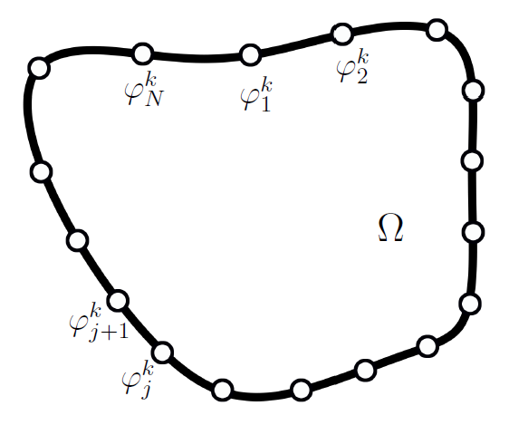
This flow may be discretely approximated as follows: Let be the step in time and be a positive constant such that represents the elapsed time. The evolving curve is represented by a set of points , here . For an illustrative diagram see Figure 8. The tangent vectors at can be approximated using a high order finite difference formula, for example
| (24) | |||||
Using Equation (24) and the assumption that for all points the quantity can be approximated by a constant when fixing , in [13] a set of formulas is presented, and they also approximate the tangent vectors and curvature :
| (25) |
Equation (23) does not have a tangential term, but an approximation for tangential vectors is needed when we reparametrize the evolution in a tubular neighborhood. By Theorem (2), we know that any reparametrization will give rise to a tangential term in the evolution equation. Then, the formula for provides the direction of this tangent field, we only need to know the coefficients of this field at each . Notice that is a first order approximation for tangential speed. Then, rescaling formula to get , it represents a numerical arc-length parametrization. In [13], the reparametrization is such that is constant for every and fixed , and the are given by
| (26) | |||||
When in Equation (23), that is isotropic mean curvature flow, an approximation for the term along the normal direction was given in [13]. Here we are concerned with finding a numerical solution to the system (P1-P2), and we seek an approximation of the form
| (27) |
Equation (26) can be used to compute the tangential component of Equation (27) for the problem (P1-P2). The normal component requires in addition the use of Proposition (12). Substituting the data of problem (P2) into equation (21), we obtain
| (28) |
The last two terms in the right side of 28 depend on the values of on the boundary . According to Theorem 10, we define implicitly through (P3). Then, in addition to (28), we need to consider Poisson’s representation formula for (P3):
| (29) |
Discretizing (28) and (29) we find two systems of linear equations. Notice that, in this case, we can solve (29) independently because there is no dependence.
In order to solve equations (28) and (29) numerically, we need to approximate the integrands on certain points. To approximate at each , we use (25) from Kimura’s numerical scheme. In general, from discrete values at and , we can determine the values for points in between by linear interpolation. This procedure is required to compute , and the normal vector for points along each arc . In contrast, Laplace’s fundamental solution and its derivatives can be substituted explicitly.
One can split the integrals in (28) and 29 into integrals over the arcs . If each arc is reparametrized by an interpolating function, all the integrals can be reduced to a linear system of equations, which can be solved numerically. Then, the procedure for (28) and (29) is to solve (29) for , and use these values to interpolate at the integrands in (28).
4. Implementation of our numerical anisotropic MCF to Contour Parametrization
For a contour parametrization problem, let be a closed planar and smooth curve drawn on a picture. In addition, suppose that the curve is enclosing a unique object in the image. We perform a curve evolution that moves the curve towards the boundary of the object. We now apply the numerical procedure in the last section to perform this evolution. First, we will describe the procedure and some assumptions we will need, and finally we will state the algorithm.
To achieve all the numerical computations we need to define a suitable function for problem (P2). As we pointed out previously, encodes the normal field which allows the curve to evolve further when . In analogy with many physical problems, suppose a point is inside , and let be the Dirac delta function. Then, let be the distribution in (P2) and in equation (28), the integral is easily computed and curve will shrink toward . At each time we need to recompute the coefficients and . Thus, there is no restriction in choosing a non fixed , as long as it remains inside the curve because the problem (P2) requires a defined in the area enclosed by . Although a non fixed may match the curve and the object faster, a stability result in such a context would be more complicated to state. The stability of our scheme will be analyzed in the next section.
As the curve evolves by equation (27), at each we can pick a pixel value. Suppose, for illustration purposes, that the picture on which the curve is evolving is in high contrast. That is, the pixels which belong to the object have a very different value from those belonging to the background. Then, we can distinguish if a point reaches the object by its pixel value.
Recalling (10), the the curve evolves by a combination of the contributions of and a standard MCF. When a point meets the object, we need to constrain its motion vanishing and its curvature . For our examples we considered black pixel objects in a white background. Let be the pixel value function, we can make and vanish through:
| (30) |
Division by 255 in the previous system of equations normalizes the Pix function, because the color intensities are usually represented by values in . Additionally, we can consider other pixel value functions depending on the number of color channels (RGB or CMYK).
To include these constraints, we summarize the previous ideas as follows:
-
I
Let , be positive, consider a set of points representing a closed planar smooth curve, a high contrast picture with a single object enclosed by the set of points, and an initial set of required to define according to (30).
-
II
Check if the set of points are in the enclosed area of . If it is not, finish procedure (or optionally, compute/ask for a new set ).
- III
-
IV
Compute the normal coefficients solving a linear system:
-
IV.a
Discretize equation (28) to obtain linear equations with unknown variables and . These equations cannot be modified because they represent (P1) and (P2). Our task is to determine the normal velocities .
- IV.b
-
IV.a
-
V
Compute the new positions substituting and into (27).
-
VI
Check how many points have reached the object using its pixel value, if most of them have reached the object (according to the set threshold), then stop.
-
VII
Return to II.
The stopping point in VI will depend on a pre-assigned threshold. We used values above 90%—explained below—for our experiments. Alternatively, one could to fix a maximum number of iterations to be carried out. This is a feature of our approach that can not be avoided, as otherwise the process will continue indefinitely.
The previous steps are distilled into the following algorithm. It has a fixed maximum possible value of of contour reached, as an example.
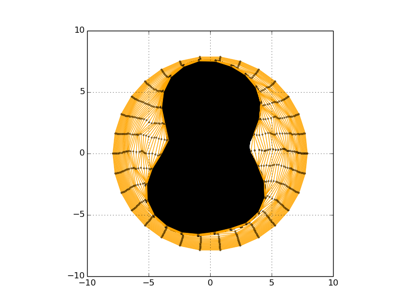
We present some examples obtained with this procedure in Figure 9 with their detailed parameters in Table 1. To estimate the accuracy in the contour detection, we compare the black pixels area and the area inside the last curve in evolution. The source code for these examples is available at https://github.com/V3du4rd0/AMCF.
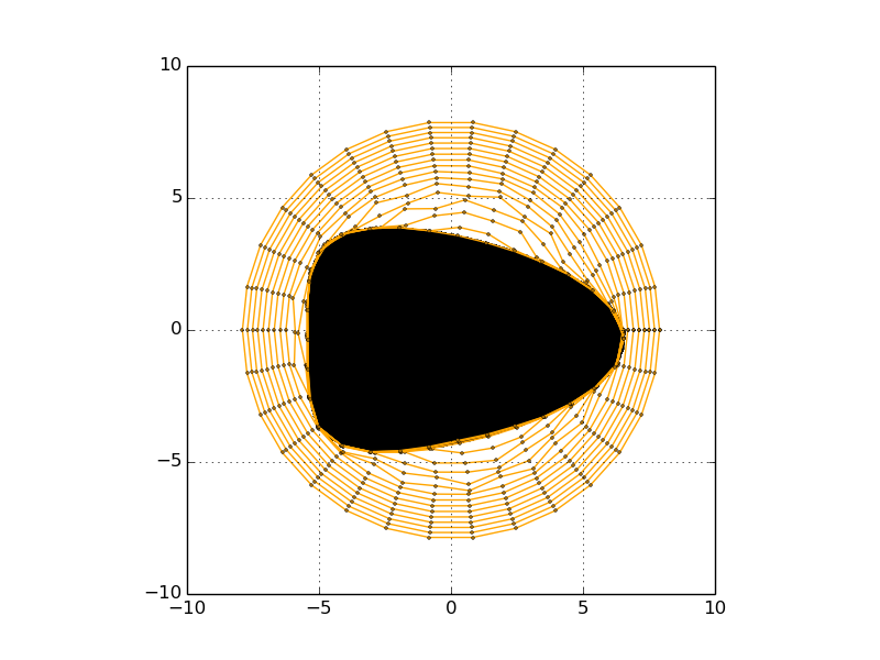
(a) (b)
| N | it. | Acc.() | |||||
|---|---|---|---|---|---|---|---|
| Fig. 9 a | 30 | 1.11 | 0.15 | 26140 | 97 | ||
| plotted each 1000 it. | |||||||
| 100 of points matched | |||||||
| Fig. 9 b | 30 | 1.11 | 0.15 | 30820 | 98 | ||
| plotted each 2000 it. | |||||||
| 100 of points matched |
Execution times
We used a small number of points to represent the evolving curve. Nevertheless, our numerical examples demand a considerable number of iterations. These iterations increase the computation time in a single processor computer. In order to reduce the execution time, we parallelized step 11, 12 and 13 in Algorithm 1. This will reduce execution times if a long number of points are needed. All the numerical experiments were performed using double precision float point arithmetic. We used Nvidia’s Jetson computer model TK1, with 2GB RAM memory, ARM A15 processor and Nvidia’s Tegra K1 graphic card with 192 CUDA cores.
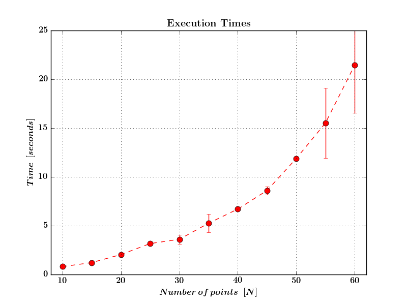
To provide a picture of how fast our process can be performed, we implement the Algorithm (1) varying the number of points and setting the time step , we plot the time versus the number of points. This (execution time) plot is presented in Figure (10). Here, the dots represent the mean time computed by taking ten samples, and the bars are the deviation of these values. The plot was obtained from a circumference as initial curve, enclosing a black circle picture with the same center. The Algorithm (1) was initialized with only one also localized in the center of the curve. The evolution was stopped when at least of the points had reached the object. These results were achieved in parallel to speed up the process.
5. Conditioning and Stability of our Numerical scheme
In this section we state our main results on the numerical analysis of the evolution scheme.
Let be the resulting matrix associated to the linear system when Equations (28) and (29) are discretized.
In order to understand the effect of the source , observe that equations (28) and (29) depend on through . As Laplace’s fundamental solution is a logarithmic function, when approaches the boundary, larger values of and its derivatives will appear for the curve points near . Consequently, these values may increase some entries in the matrix in the linear system. Therefore, the matrix norm may change drastically when is lower than one because
The condition number of a matrix with the norm is thereby affected:
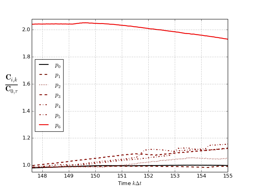
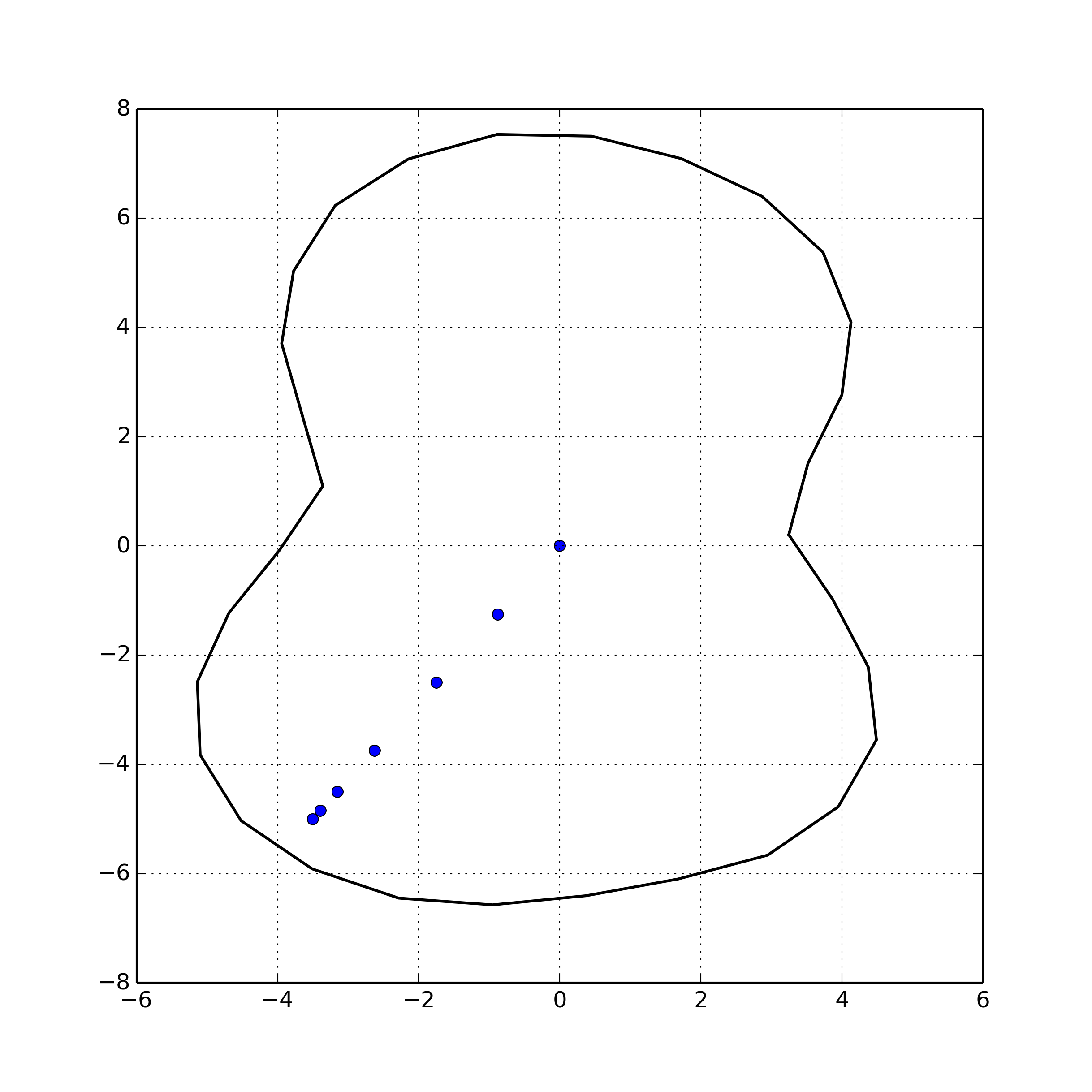
Let be a set of source coordinates. Denote by the condition number of at time when . We now repeat example a in Figure 9 for different charge positions , from to . In Figure (11) we present how the condition number increases as approaches the curve, the condition number when is at is used as reference (). Notice in Figure 11 that the highest values of are obtained for , which corresponds to the point () which is closest to boundary.
(a) (b)
Remark. In order to maximize the distance between and the curve in a convex contour parameterization problem, a suitable choice of at time is the centroid coordinates of the set . Further investigating other possible choices of placement for the charge in the general case, or increasing the number of charges, constitutes an interesting avenue for future research, and lies outside the scope of our work here.
We now focus on the stability of the updating scheme
| (31) |
Let be the curve at time represented by a set of points , its length is approximated by . We will rewrite the tangential and normal vectors in (31) and thus obtain a expression only in terms of the set . Recall the definitions of and :
| (32) | |||||
Therefore
| (33) |
To determine the numerical error propagation in (31), let be an exact solution of system (P1), (P2) and (P3), then all points must satisfy (31). If another initial representation of the same curve evolves, the final positions in both sets may represent different curves, because the approximation errors in each set propagate differently. The core in the following analysis is to compare the error amplification when the relative distances change, and this is crucial for the stability as the evolving curves shrink along the flow.
Let be the exact solution, and let be another discrete representation of the same evolving curve with uniformly distributed points. Suppose that both sets have one point in common. The difference between these sets is the number of points, this condition prevents us to compare the coordinates point-wise, except for the common point and when the same time has elapsed.
As is an exact solution of the system (P1), (P2) and (P3), then it must satisfy (31). At the time , the coordinates for the common point will differ by a small error
| (34) |
denoting by , we point out that except for . We will get an equation for in terms on the error in the additional parameters:
and so on for and in . Notice that, even when , and therefore , the previous parameters depend non linearly on other points. Thus, the coefficients which drive the evolution ( and ) are different for and .
Since both sets of points are uniformly distributed at time , then . We can now rewrite Equation 31:
Remark. We cancel the tangential terms because the points are uniformly distributed at time , but in further iterations, for example , this is not possible in general. Consequently, this analysis determines whether choosing a different number of points is appropriate to reduce the error amplification only for the next time step. If we do not assume this uniform tangential distribution, the resulting equation will be complicated to analyze, even when (31) is linearized, because it would then depend on the projection of along the segments for all .
Recall that is an exact solution, so the last equation implies:
| (35) |
To obtain an explicit expression for (35), we need the following computations:
Assuming that the difference between and is small, we linearize . Then,
To simplify a future computation, we write the vectors in terms of and :
here
Additionally, we write in terms of and :
Later on, we will bound these constants. Let and be the identity matrix, define
we can now rewrite Equation 35
| (36) | |||||
As the curve is closed, we can assume that is periodic of period over the curve. Von Neumann’s theory implements Fourier analysis to determine whether the error remains bounded as time elapses. The discrete representation of the curve requires us to consider the discrete Fourier transformation of in the spatial coordinate and with periodic conditions. From Fourier analysis, can be written using the inverse Fourier transformation as
Thus
| (37) |
After substituting into (36) we find
| (38) |
Here
Equation (38) defines a formula from which we deduce in terms of . However, this formula is not recursive because the matrix entries depend on time through and . Let be given by
Then, using von Neumann’s analysis we can only determine how much does the error is being amplified at the next time step. To proceed with this analysis, we need for to remain bounded in the consecutive step. Therefore, we will compute the eigenvalues and of . Letting and be the associated eigenvectors, then can be written in terms of and . Consequently, we will guarantee that does not grow by finding the constraints on , such that the eigenvalues are bounded absolutely by one.
Let , and let , be the eigenvalues of . Then, the eigenvalue moduli are
| (39) |
| (40) |
From now, we will only consider the amplification of the worse possible error. This error amplification can be obtained by considering the maximum of and replacing the values of sine and cosine above by 1 or -1, in that order.
As the points lie equidistantly, and do not overlap we find:
In addition,
We consider the following bounds using and
Assuming that the size of errors is almost the same for . Then, the norm of the eigenvalues in (39) and (40) can be bounded by
| (41) |
Remark. The number of points that represents the curve determines the integral discretization, because we split the integral over into integrals over the arcs . However, all these integrals are computed by an approximation formula, and therefore this error propagates to , we called this error . Some well-known accurate formulas can be used to bound this integration error, in all numerical experiments we used the 3-points Gaussian Quadrature Formula. The accuracy of these formulas increase with the number of interpolated points. To proceed with the analysis, we will disregard in (41).
Proposition 13.
Let and be two discrete representations of the same curve evolving by P1, P2 and P3. Then the representation with the least number of points will produce lower error amplification.
Proof.
Using Equation 41, and dealing with according to the last remark:
We are using Kimura’s uniform tangential redistribution scheme, so we are constrained to set . Therefore,
Noticing that this norm will be minimized if , we conclude the proof. ∎
Remark. Proposition 13 only assumes two different representations of the same curve. Nevertheless, the use of the bound found in (41) assumes that and do not differ overly because we linearized the inverse of relative distances to get the bounds. Additionally, we suppose that both representations are suitable in the sense that the sum over the polygonal distances approximates the curve length, because the numerical integration depends on this hypothesis in order to handle .
6. Conclusions
We presented a novel anisotropic mean curvature geometric flow together with an implementation of it through a numerical scheme, applied to contour recognition tasks. Our proposal has the following features: (1) The curve evolution is given by an explicit scheme. Consequently, the required resolution for the contour recognition can used to choose the size of the stored data array. (2) The stability of our scheme can only be checked at each iteration using the explicit values of , and , according to Proposition 13. (3) We provided specific criteria to improve the conditioning and to verify the stability of this method at each time step.
Moreover, the implementation was optimized to run in parallel, and the code has been made publicly available.
Future improvements for this method may include increasing of the number of point charges that drive the curve evolution, and inferring optimal distributions and values for the potentials. Due to the unavailability of implementations—for example accesible in code repositories—of previous methods, we defer comprehensive comparisons with other schemes of numerical mean curvature flows [24, 25, 1].
References
- [1] Martin Balazovjech and Karol Mikula. A higher order scheme for a tangentially stabilized plane curve shortening flow with a driving force. SIAM Journal on Scientific Computing, 33(5):2277–2294, 2011.
- [2] Kenneth A. Brakke. The Motion of a Surface by Its Mean Curvature. (MN-20). Princeton University Press, 1978.
- [3] Martin Burger, Yanina Landa, Nicolay M. Tanushev, and Richard Tsai. Algorithmic Foundation of Robotics VIII: Selected Contributions of the Eight International Workshop on the Algorithmic Foundations of Robotics. Springer Berlin Heidelberg, Berlin, Heidelberg, 2010.
- [4] Bing-Long Chen. Uniqueness and pseudolocality theorems of the mean curvature flow. Communications in Analysis and Geometry, 15(3):435–490, 2007.
- [5] David L. Chopp and James A. Sethian. Flow under curvature: singularity formation, minimal surfaces, and geodesics. Experiment. Math., 2(4):235–255, 1993.
- [6] B. Chow, S.C. Chu, D. Glickenstein, C. Guenther, J. Isenberg, T. Ivey, D. Knopf, P. Lu, F. Luo, and L. Ni. The Ricci Flow: Techniques and Applications:. Mathematical Surveys and Monographs. American Mathematical Society, 2015.
- [7] K. Ecker. Regularity Theory for Mean Curvature Flow. Progress in Nonlinear Differential Equations and Their Applications. Birkhäuser Boston, 2012.
- [8] L.C. Evans. Partial Differential Equations. Graduate studies in mathematics. American Mathematical Society, 2010.
- [9] G.B. Folland. Introduction to Partial Differential Equations. Princeton University Press, 1995.
- [10] Huisken Gerhard and Polden Alexander. Calculus of Variations and Geometric Evolution Problems: Lectures given at the 2nd Session of the Centro Internazionale Matematico Estivo (C.I.M.E.) held in Cetraro, Italy, June 15–22, 1996. Springer Berlin Heidelberg, Berlin, Heidelberg, 1999.
- [11] P. Hájek and M. Johanis. Smooth analysis in Banach spaces. De Gruyter Series in Nonlinear Analysis and Applications. De Gruyter, 2014.
- [12] Michael Kass, Andrew Witkin, and Demetri Terzopoulos. Snakes: Active contour models. International Journal of Computer Vision, 1(4):321–331, 1988.
- [13] Masato Kimura. Numerical analysis of moving boundary problems using the boundary tracking method. Japan Journal of Industrial and Applied Mathematics, 14(3):373–398.
- [14] S.G. Krantz. Geometric Function Theory: Explorations in Complex Analysis. Cornerstones. Birkhäuser Boston, 2007.
- [15] R.J. LeVeque. Finite Difference Methods for Ordinary and Partial Differential Equations: Steady-State and Time-Dependent Problems. Society for Industrial and Applied Mathematics, 2007.
- [16] Leevan Ling, Y. C. Hon, and M. Yamamoto. Inverse source identification for poisson equation. Inverse Problems in Science and Engineering, 13(4):433–447, 2005.
- [17] R. Malladi and J.A. Sethian. Image processing: Flows under min/max curvature and mean curvature. Graphical Models and Image Processing, 58(2):127 – 141, 1996.
- [18] C. Mantegazza. Lecture Notes on Mean Curvature Flow. Progress in Mathematics. Springer Basel, 2011.
- [19] W. W. Mullins. Two-dimensional motion of idealized grain boundaries. Journal of Applied Physics, 27(8):900–904, 1956.
- [20] Takashi Ohe and Kohzaburo Ohnaka. Boundary element approach for an inverse source problem of the poisson equation with a one-point-mass like source. Applied Mathematical Modelling, 18(4):216 – 223, 1994.
- [21] S. Osher and R. Fedkiw. Level Set Methods and Dynamic Implicit Surfaces. Applied Mathematical Sciences. Springer, 2003.
- [22] R.H. Pletcher, J.C. Tannehill, and D. Anderson. Computational Fluid Mechanics and Heat Transfer, Third Edition. Series in Computational and Physical Processes in Mechanics and Thermal Sciences. CRC Press, 2016.
- [23] S.A. Sauter and C. Schwab. Boundary Element Methods. Springer Series in Computational Mathematics. Springer Berlin Heidelberg, 2010.
- [24] J.A. Sethian. Level Set Methods and Fast Marching Methods: Evolving Interfaces in Computational Geometry, Fluid Mechanics, Computer Vision, and Materials Science. Cambridge Monographs on Applied and Computational Mathematics. Cambridge University Press, 1999.
- [25] Daniel Ševčovič and Shigetoshi Yazaki. Evolution of plane curves with a curvature adjusted tangential velocity. Japan Journal of Industrial and Applied Mathematics, 28(3):413, 2011.
- [26] E. Pedersen T. Colding, W. Minicozzi. Mean curvature flow. Bull. Amer. Math. Soc., 52:297 – 333, 2015.
- [27] Z. Wu, J. Yin, and C. Wang. Elliptic & Parabolic Equations. World Scientific, 2006.
- [28] E. Zeidler. Nonlinear Functional Analysis and Its Applications: Fixed point theorems. Nonlinear Functional Analysis and Its Applications. Springer-Verlag, 1985.
- [29] E. Zeidler and L.F. Boron. Nonlinear Functional Analysis and Its Applications: II/ A: Linear Monotone Operators. Monotone operators / transl. by the author and by Leo F. Boron. Springer New York, 1989.
- [30] X.P. Zhu. Lectures on Mean Curvature Flows. AMS/IP studies in advanced mathematics. American Mathematical Soc.