Current fluctuations in quantum absorption refrigerators

Abstract

Absorption refrigerators transfer thermal energy from a cold bath to a hot bath without input power by utilizing heat from an additional “work” reservoir. Particularly interesting is a three-level design for a quantum absorption refrigerator, which can be optimized to reach the maximal (Carnot) cooling efficiency. Previous studies of three-level chillers focused on the behavior of the averaged cooling current. Here, we go beyond that and study the full counting statistics of heat exchange in a three-level chiller model. We explain how to obtain the complete cumulant generating function of the refrigerator in steady state, then derive a partial cumulant generating function, which yields closed-form expressions for both the averaged cooling current and its noise. Our analytical results and simulations are beneficial for the design of nanoscale engines and cooling systems far from equilibrium, with their performance optimized according to different criteria, efficiency, power, fluctuations and dissipation.

I Introduction

Autonomous absorption refrigerators transfer thermal energy from a cold ($c$) bath to a hot ($h$) bath by utilizing heat from an ultra-hot heat bath, termed as a work ($w$) reservoir. Absorption refrigerators were realized in the 19th century AR19 , and their analysis was central to the development of the theory of finite-time irreversible thermodynamics. Theoretical studies of quantum, nanoscale analogues of absorption refrigerators aim to establish the theory of macroscopic thermodynamics from quantum principles review1 ; kos13 ; reviewARPC14 ; Goold ; kos18 . Recent experiments demonstrated classical nanoscale engines, e.g. a single atom heat engine singleatom and a nanomechanical heat engine utilizing squeezed thermal reservoirs squeezeE . More recently, a quantum absorption refrigerator was realized using three trapped ions QARE .

An illustrious design of an autonomous quantum absorption refrigerator (QAR) consists of a three-level system as the working fluid and three independent thermal reservoirs reviewARPC14 ; joseSR . Each transition between a pair of levels is coupled to one of the three heat baths, $c$, $h$ and $w$, where $T_{w}>T_{h}>T_{c}$. For a schematic representation, see Fig. 1. In the steady state limit, the work bath provides energy to the system promoting the extraction of energy from the cold bath, to be dumped into the hot reservoir. The opposite heating process, from the hot bath to the cold one, can be controlled and played down by manipulating the frequencies of the system.

The three-level QAR and its variants were discussed in details in several recent studies, see e.g. Refs. reviewARPC14 ; joseSR ; Levy12 ; Linden11 ; plenio ; PopescuPRL ; Popescu12 ; Alonso14 ; jose15 ; AlonsoNJP . It is designed to perform optimally under the weak coupling approximation, when each bath individually couples to a different transition within the system. Quantum coherences are expected to negatively impact the cooling performance of multilevel QARs by introducing internal dissipation and leakage processes jose15 . Off-resonant effects and bath-cooperative interactions may contribute to energy exchange once the system strongly interacts with the thermal baths. Such nonlinear effects are difficult to control and can lead to a rather poor performance. In a recent study we had analyzed a qubit QAR by making the system to strongly interact with three shaped reservoirs Anqi . Carnot efficiency was then achieved in a singular design—with the baths engineered to consist only specific frequency components. The three-level QAR and similar continuous (non-reciprocating) machines can be realized in different physical systems including coupled atoms and ions, multi-site electronic junctions and photovoltaic cells, as described e.g. in Refs. plenio ; NitzanE1 ; KilgourD .

Figure 1: A three-level quantum absorption refrigerator. It includes a quantum system (working fluid) with each transition coupled to an independent thermal bath, hot ($h$), cold ($c$) and work ($w$).

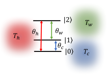
Beyond the analysis of the averaged cooling current, a full counting statistics (FCS) formalism provides the fundamental description of an out-of-equilibrium quantum system esposito-review ; hanggi-review ; bijay-wang-review . Such an approach hands over the cumulant generating function (CGF) for heat exchange, fully characterizing energy transport in steady state. The goal of the present paper is to employ a full counting statistics formalism and study the cooling performance of a three-level QAR.

The paper includes three central contributions: (i) We describe the calculation of the FCS of heat exchange in the three-level QAR. (ii) We introduce a practical method for reaching closed-form expressions for the first two cumulants (cooling current and its noise) through the derivation of a partial CGF. The method is general and can be readily applied to other multilevel models beyond the weak coupling approximation. (iii) We simulate the behavior of the cooling current, its noise and the accuracy-dissipation trade off. Altogether, these measures are important for the optimization of heat machines vanden16 ; TUR1 ; TUR2 ; TUR3a ; TUR3b ; Geissler .

The work is organized as follows. We introduce our model in Sec. II. In Sec. III we present the FCS approach and derive expressions for the cooling current and its noise. We illustrate our results with numerical simulations in Sec. IV and summarize in Sec. V.

II Model

The paradigmatic three-level QAR is described by the Hamiltonian $\hat{H}=\hat{H}_{s}+\hat{H}_{b}+\hat{H}_{sb}$ with a three-level system $\hat{H}_{s}=\sum_{0,1,2}E_{j}|j\rangle\langle j|$ and three reservoirs $\hat{H}_{b}=\hat{H}_{c}+\hat{H}_{w}+\hat{H}_{h}$. The baths include collections of independent harmonic oscillators, $\hat{H}_{\nu}=\sum_{k}\omega_{\nu,k}a_{\nu,k}^{\dagger}a_{\nu,k}$, with $a_{\nu,k}^{\dagger}$ ($a_{\nu,k}$) the creation (annihilation) operator of mode $k$ with frequency $\omega_{\nu,k}$ in the $\nu=h,c,w$ bath. Each thermal bath is coupled to a specific transition within the system,

$$\hat{H}_{sb} = \hat{B}_{c}\left(|0\rangle\langle 1|+|1\rangle\langle 0|\right)+\hat{B}_{w}\left(|1\rangle\langle 2|+|2\rangle\langle 1|\right)$$ (1)

$$+ \hat{B}_{h}\left(|0\rangle\langle 2|+|2\rangle\langle 0|\right).$$

The bath operators are $\hat{B}_{\nu}=\sum_{k}g_{\nu,k}\left(a_{\nu,k}^{\dagger}+a_{\nu,k}\right)$, but the analysis can be readily generalized beyond that. In what follows we use the notation $\theta_{c}\equiv E_{1}-E_{0}$, $\theta_{w}\equiv E_{2}-E_{1}$ and $\theta_{h}\equiv\theta_{c}+\theta_{w}$.

The dynamics of the reduced density matrix can be organized as a Markovian quantum master equation for the levels’ populations under the following assumptions Breuer : (i) weak system-bath coupling, (ii) Markovian reservoirs, and (iii) decoupled coherences-population dynamics (secular approximation). This standard scheme results in the following kinetic-like equations

$$\dot{p}_{0} = -\left(k_{0\to 1}+k_{0\to 2}\right)p_{0}(t)+k_{1\to 0}p_{1}(t)+k_{2\to 0}p_{2}(t),$$

$$\dot{p}_{1} = -\left(k_{1\to 0}+k_{1\to 2}\right)p_{1}(t)+k_{0\to 1}p_{0}(t)+k_{2\to 1}p_{2}(t),$$

$$\dot{p}_{2} = -\left(k_{2\to 0}+k_{2\to 1}\right)p_{2}(t)+k_{0\to 2}p_{0}(t)+k_{1\to 2}p_{1}(t),$$

with rate constants

$$k_{0\to 1} = \Gamma_{c}(\theta_{c})n_{c}(\theta_{c}),\,\,\,k_{0\to 2}=\Gamma_{h}(\theta_{h})n_{h}(\theta_{h}),$$

$$k_{1\to 2} = \Gamma_{w}(\theta_{w})n_{w}(\theta_{w}).$$ (3)

The detailed balance relation dictates the rate constants of reversed processes, e.g., $k_{1\to 0}=\Gamma_{c}(\theta_{c})\left[n_{c}(\theta_{c})+1\right]$. The system-bath coupling constants (hybridization) are $\Gamma_{\nu}(\theta_{\nu})=2\pi\sum_{k}|g_{\nu,k}|^{2}\delta(\omega_{\nu,k}-\theta_{\nu})$, and we used an ohmic function to model them, $\Gamma_{\nu}(\theta_{\nu})=\theta_{\nu}$. The Bose-Einstein occupation factors are $n_{\nu}(\theta_{\nu})=[e^{\beta_{\nu}\theta_{\nu}}-1]^{-1}$, given in terms of the inverse temperature $\beta_{\nu}=1/(k_{B}T_{\nu})$. In the weak-coupling approximation employed here only resonance processes are allowed. For brevity, we omit below the reference to frequency in $\Gamma_{\nu}(\theta_{\nu})$ and $n_{\nu}(\theta_{\nu})$.

Our equations of motion can be written in terms of the dissipators $L_{\nu}$ as $|\dot{p}\rangle=(L_{c}+L_{h}+L_{w})|p(t)\rangle$, with $|p\rangle$ a vector of population and $\sum_{j}p_{j}(t)=1$. This equation can be solved in the long time limit, yielding the steady state population, $p_{j}^{ss}$. The rate of change of the system’s energy is given by $d\langle\hat{H}_{s}\rangle/dt$. From here, we can immediately write down a closed-form expression for the averaged energy current at the $\nu$ contact, namely $\langle J_{\nu}\rangle=\sum_{j}(L_{\nu}|p^{ss}\rangle)_{j}E_{j}$. This procedure was employed in previous studies, see e.g. reviewARPC14 ; joseSR . In the next section we generalize this description by using a full counting statistics analysis, and explicitly calculate the first two cumulants.

III Full Counting Statistics

III.1 The complete CGF

The cumulant generating function of the model described in Sec. II can be derived by following a rigorous procedure esposito-review ; hava . Here, for simplicity, we employ a classical, intuitive derivation of the FCS; it complies with the rigorous method under the weak-coupling, Markovian and secular approximations hava . We begin by defining $\mathcal{P}_{t}(j,n\theta_{c},m\theta_{w})$ as the probability that by the time (long time) $t$, a total energy $n\theta_{c}$ has been absorbed by the system from the cold bath, $m\theta_{w}$ energy has been transferred from the work bath to the system, and the system populates the state $j=0,1,2$. Since the dynamics is Markovian and energy is conserved, we do not count energy at the third bath. Note that $n,m$ are integers since under the weak coupling (resonant transmission) approximation, heat is transferred into and out of the system in discrete quanta $\theta_{c,w,h}$. We can readily write down an equation of motion for $\mathcal{P}_{t}(j,n\theta_{c},m\theta_{w})$ esposito-review ; Renjie ; yelenaPRB ; yelenaCGF ,

$$\dot{\mathcal{P}}_{t}(0,n\theta_{c},m\theta_{w}) = -\mathcal{P}_{t}(0,n\theta_{c},m\theta_{w})(k_{0\rightarrow 1}+k_{0\rightarrow 2})+\mathcal{P}_{t}(1,(n+1)\theta_{c},m\theta_{w})k_{1\rightarrow 0}+\mathcal{P}_{t}(2,n\theta_{c},m\theta_{w})k_{2\rightarrow 0},$$

$$\dot{\mathcal{P}}_{t}(1,n\theta_{c},m\theta_{w}) = -\mathcal{P}_{t}(1,n\theta_{c},m\theta_{w})(k_{1\rightarrow 0}+k_{1\rightarrow 2})+\mathcal{P}_{t}(0,(n-1)\theta_{c})k_{0\rightarrow 1}+\mathcal{P}_{t}(2,n\theta_{c},(m+1)\theta_{w})k_{2\rightarrow 1},$$

$$\dot{\mathcal{P}}_{t}(2,n\theta_{c},m\theta_{w}) = -\mathcal{P}_{t}(2,n\theta_{c},m\theta_{w})(k_{2\rightarrow 0}+k_{2\rightarrow 1})+\mathcal{P}_{t}(1,n\theta_{c},(m-1)\theta_{w})k_{1\rightarrow 2}+\mathcal{P}_{t}(0,n\theta_{c},m\theta_{w})k_{0\rightarrow 2}.$$ (4)

Figure 2: Real (Re) and imaginary (Im) parts of the cumulant generating function $G(\chi_{c},\chi_{w}=0)$. (a) Complete CGF computed from a numerical solution of the eigenvalue problem, Eqs. (6)-(14). (b) Deviation of the first order CGF $G^{(1)}(\chi)$ of Eq. (17) from the complete CGF. (c) Deviation of the second order CGF $G^{(2)}(\chi)$ of Eq. (24) from the complete CGF. We used $\beta_{c}=1$, $\beta_{w}=0.2$, $\beta_{h}=0.7$, $\theta_{h}=6$, and we varied $\theta_{c}$ up to $\theta_{h}$.

We Fourier-transform these equations by introducing the the so-called counting fields $\chi=(\chi_{c},\chi_{w})$, and obtain the characteristic function

$$\ket{Z(\chi,t)}\equiv$$

$$\begin{pmatrix}\sum_{n,m=-\infty}^{\infty}\mathcal{P}_{t}(0,n\theta_{c},m\theta_{w})e^{in\theta_{c}\chi_{c}}e^{im\theta_{w}\chi_{w}}\ \\ \sum_{n,m=-\infty}^{\infty}\mathcal{P}_{t}(1,n\theta_{c},m\theta_{w})e^{in\theta_{c}\chi_{c}}e^{im\theta_{w}\chi_{w}}\ \\ \sum_{n,m=-\infty}^{\infty}\mathcal{P}_{t}(2,n\theta_{c},m\theta_{w})e^{in\theta_{c}\chi_{c}}e^{im\theta_{w}\chi_{w}}\ \end{pmatrix}$$

(5)

It satisfies a first order differential equation,

$$\frac{d|Z(\chi,t)\rangle}{dt}=\hat{W}(\chi)|Z(\chi,t)\rangle$$ (6)

with the rate matrix

$$\hat{W}=\begin{pmatrix}-k_{0\rightarrow 1}-k_{0\rightarrow 2}&k_{1\rightarrow 0}e^{-i\chi_{c}\theta_{c}}&k_{2\rightarrow 0}\\ k_{0\rightarrow 1}e^{i\chi_{c}\theta_{c}}&-k_{1\rightarrow 0}-k_{1\rightarrow 2}&k_{2\to 1}e^{-i\chi_{w}\theta_{w}}\\ k_{0\rightarrow 2}&k_{1\rightarrow 2}e^{i\chi_{w}\theta_{w}}&-k_{2\rightarrow 1}-k_{2\to 0}\\ \end{pmatrix}$$

(7)

The characteristic polynomial of $\hat{W}$ is written schematically as

$$\lambda^{3}-a_{1}\lambda^{2}+a_{2}\lambda-a_{3}(\chi)=0,$$ (8)

with the eigenvalues $\lambda_{1,2,3}$ sorted from the smallest in magnitude to largest by their real part. The coefficients of the polynomial are given by

$$a_{1} = w_{0,0}+w_{1,1}+w_{2,2},$$

$$a_{2}(\chi) = w_{0,0}w_{1,1}+w_{0,0}w_{2,2}+w_{1,1}w_{2,2}$$

$$- w_{0,1}(\chi_{c})w_{1,0}(\chi_{c})-w_{0,2}w_{2,0}-w_{1,2}(\chi_{w})w_{2,1}(\chi_{w}),$$

$$a_{3}(\chi) = w_{0,0}w_{1,1}w_{2,2}-w_{0,0}w_{1,2}(\chi_{w})w_{2,1}(\chi_{w})$$ (9)

$$- w_{0,1}(\chi_{c})w_{1,0}(\chi_{c})w_{2,2}+w_{0,1}(\chi_{c})w_{1,2}(\chi_{w})w_{2,0}$$

$$+ w_{0,2}w_{2,1}(\chi_{w})w_{1,0}(\chi_{c})-w_{0,2}w_{2,0}w_{1,1}.$$

Here, $w_{m,n}$ are the matrix elements of $\hat{W}(\chi)$ in Eq. (7), with the rows and columns counted by 0,1,2. It is important to note that the counting field dependence disappears within the products $w_{0,1}(\chi_{c})w_{1,0}(\chi_{c})$ and $w_{1,2}(\chi_{w})w_{2,1}(\chi_{w})$. As a result, $a_{2}$ in fact does not depend on the counting fields. Explicitly, in terms of the transition rate constants we find that

$$a_{1} = -\Gamma_{c}\left(2n_{c}+1\right)-\Gamma_{h}\left(2n_{h}+1\right)-\Gamma_{w}\left(2n_{w}+1\right),$$

$$a_{2} = \left(\Gamma_{c}n_{c}+\Gamma_{h}n_{h}\right)\left[\Gamma_{c}(n_{c}+1)+\Gamma_{w}n_{w}\right]$$

$$+ \left[\Gamma_{c}n_{c}+\Gamma_{h}n_{h}\right]\left[\Gamma_{w}(n_{w}+1)+\Gamma_{h}(n_{h}+1)\right]$$

$$+ \left[\Gamma_{c}(n_{c}+1)+\Gamma_{w}n_{w}\right]\left[\Gamma_{w}(n_{w}+1)+\Gamma_{h}(n_{h}+1)\right]$$

$$- \Gamma_{c}^{2}(n_{c}+1)n_{c}-\Gamma_{h}^{2}(n_{h}+1)n_{h}-\Gamma_{w}^{2}(n_{w}+1)n_{w}.$$

The coefficient $a_{3}$ has two contributions that depend on $\chi$, while the rest of the expression is lumped into the constant $C$,

$$a_{3}(\chi) = w_{0,1}(\chi_{c})w_{1,2}(\chi_{w})w_{2,0}+w_{0,2}w_{2,1}(\chi_{w})w_{1,0}(\chi_{c})+C$$ (11)

$$= \Gamma_{c}\Gamma_{w}\Gamma_{h}(n_{c}+1)e^{-i\theta_{c}\chi_{c}}(n_{w}+1)e^{-i\theta_{w}\chi_{w}}n_{h}$$

$$+ \Gamma_{c}\Gamma_{w}\Gamma_{h}(n_{h}+1)n_{w}n_{c}e^{i\theta_{c}\chi_{c}}e^{i\theta_{w}\chi_{w}}+C.$$

It is useful to note that $a_{2}>0$ and that $a_{3}(\chi=0)=0$.

The cumulant generating function $G(\chi)$ is formally defined as

$$G(\chi)=\lim_{t\to\infty}\ \frac{1}{t}\ln\sum_{j}\sum_{n,m}\mathcal{P}_{t}(j,n\theta_{c},m\theta_{w})e^{in\theta_{c}\chi_{c}}e^{im\theta_{w}\chi_{w}}.$$

In terms of the characteristic function it is given by

$$G(\chi)=\lim_{t\to\infty}\ \frac{1}{t}\ln\langle I|Z(\chi,t)\rangle,$$ (13)

with $\langle I|=\langle 111|$ a unit left vector. To obtain the CGF we diagonalize $\hat{W}(\chi)$ and extract the eigenvalue that dictates the long-time dynamics—this is the eigenvalue with the smallest magnitude for its real part,

$$G(\chi)=\lambda_{1}(\chi).$$ (14)

We refer to this solution as the “complete CGF”. For 3$\times 3$ or larger matrices the diagonalization of $\hat{W}$ is performed numerically, possibly suffering from accuracy and stability issues. It is easy to verify that $a_{3}$ satisfies the exchange fluctuation symmetry

$$a_{3}(\chi_{c},\chi_{w})=a_{3}(i(\beta_{h}-\beta_{c})-\chi_{c},i(\beta_{h}-\beta_{w})-\chi_{w}),$$

(15)

which is a microscopic verification of the second law of thermodynamics esposito-review . The CGF provides e.g. the currents ($\nu=c,w$) and the noise terms as

$$\langle J_{\nu}\rangle = \frac{\partial G}{\partial(i\chi_{\nu})}\Big{|}_{\chi=0},$$

$$\langle S_{\nu}\rangle = \frac{\partial^{2}G}{\partial(i\chi_{\nu})^{2}}\Big{|}_{\chi=0}.$$ (16)

While we can reach these coefficients numerically, we are interested here in closed-form expressions. Nevertheless, acquiring analytically the roots of a cubic (or higher order) characteristic function is obviously not a trivial task. To bypass this challenge, next we illustrate that by truncating the characteristic equation (8) we reach partial CGFs, which are simple to solve and yield analytical expressions for the current and its noise.

In fact, this idea was introduced earlier on for the calculation of the diffusion coefficient in Ref. Koza . A recent application of this principle in the context of chemical kinetics was discussed in Ref. Udo-Fano . Nevertheless, here we emphasize that partial CGFs are thermodynamically consistent (maintaining the fluctuation relation), show that a partial $n$th-order CGFs can approximate cumulants beyond that order, and derive analytical expressions for the current and its noise for the canonical three-level QAR model.

III.2 First order CGF

To obtain the first cumulant, namely energy currents, it is sufficient to keep only the linear term in $\lambda$ within the polynomial (8). This linear order CGF satisfies the symmetry relation (15), and it is given by

$$G^{(1)}(\chi_{c},\chi_{w})=\frac{a_{3}(\chi_{c},\chi_{w})}{a_{2}}.$$ (17)

The heat current from the cold bath towards the system immediately follows by taking a derivative with respect to $(i\chi_{c})$ and using Eq. (11),

$$\langle J_{c}\rangle=-\frac{\theta_{c}\Gamma_{c}\Gamma_{w}\Gamma_{h}\left[(n_{c}+1)(n_{w}+1)n_{h}-(n_{h}+1)n_{w}n_{c}\right]}{a_{2}}.$$

(18)

We proceed and derive a cooling condition, $\langle J_{c}\rangle\geq 0$,

$$e^{-\beta_{c}\theta_{c}}e^{-\beta_{w}\theta_{w}}-e^{-\beta_{h}\theta_{h}}\geq 0,$$ (19)

which translates to

$$\frac{\theta_{c}}{\theta_{h}}\leq\frac{\beta_{h}-\beta_{w}}{\beta_{c}-\beta_{w}}.$$ (20)

We can similarly organize an expression for $\langle J_{w}\rangle$: Back to Eq. (17), we take the first derivative with respect to $(i\chi_{w})$. It is obvious that $\langle J_{w}\rangle$ is given by (18)—with $\theta_{w}$ replacing $\theta_{c}$. As a result, the coefficient of performance (sometimes termed cooling efficiency) reduces to

$$\eta\equiv\langle J_{c}\rangle/\langle J_{w}\rangle=\theta_{c}/\theta_{w}.$$ (21)

While these results were received before reviewARPC14 ; Levy12 ; joseSR , in our approach we accomplish them rather instantly. It is important to note that since we truncate the characteristic function to linear order in $\lambda$, our results are accurate for the heat current, but the current noise is incomplete.

Reorganizing the cooling condition (20) we get

$$\theta_{c}/\theta_{w}\leq(\beta_{h}-\beta_{w})/(\beta_{c}-\beta_{h}),$$ (22)

which translates to $\eta\leq\eta_{c}$, with the Carnot COP identified as $\eta_{c}=\frac{\beta_{h}-\beta_{w}}{\beta_{c}-\beta_{h}}$. This bound was derived in Ref. bijayS based on a full counting statistics approach. This maximal COP is achieved when the cooling current (18) diminishes. The heat currents $\langle J_{h,w}\rangle$ nullify at that point as well, with zero entropy production rate. Beyond that, the three-level QAR described in this work is an endoreversible heat machine: finite heat transfer rates between the working fluid and the reservoirs reduce the efficiency below the Carnot bound.

Figure 3: (a)-(d) Cooling current and noise of the three-level QAR as a function of $\theta_{c}=\theta_{h}-\theta_{w}$. We fix $\beta_{c}=1$, $\beta_{w}=0.1$, $\theta_{h}=6$, and tune $\beta_{h}$ from high (panel a) to low (panel (d)) temperature. The boundary of the cooling window is marked by a circle.

Figure 4: (a)-(d) Thermodynamic uncertainty relation (full) along with its bound of 2 (dotted), $k_{B}\equiv 1$. In the bottom panels we display the coefficient of performance $\theta_{c}/\theta_{w}$ (dashed) and its maximal Carnot value (dotted), $\eta_{C}=(\beta_{h}-\beta_{w})/(\beta_{c}-\beta_{h})$. Parameters are the same as in Fig. 3. The boundary of the cooling window is marked by a circle.

III.3 Second order CGF

To derive a closed-form expression for the second cumulant, the current noise, we need to retain the quadratic term in the polynomial equation (8),

$$\lambda^{2}-\frac{a_{2}}{a_{1}}\lambda+\frac{a_{3}(\chi)}{a_{1}}=0.$$ (23)

The resulting-partial CGF is given by the root with the smallest-magnitude real part,

$$G^{(2)}(\chi)=\frac{a_{2}-\sqrt{a_{2}^{2}-4a_{3}(\chi)a_{1}}}{2a_{1}}.$$ (24)

This partial CGF preserves the fluctuation symmetry. By taking the first and second derivatives with respect to $\chi_{c}$, we derive expressions for the cooling current and its noise,

$$\langle J_{c}\rangle = \frac{1}{a_{2}}\frac{\partial a_{3}}{\partial(i\chi_{c})}\Big{|}_{\chi=0},$$

$$\langle S_{c}\rangle = \frac{1}{a_{2}}\left[\frac{\partial^{2}a_{3}}{\partial(i\chi_{c})^{2}}+\frac{2a_{1}}{a_{2}^{2}}\left(\frac{\partial a_{3}}{\partial(i\chi_{c})}\right)^{2}\right]\Bigg{|}_{\chi=0},$$ (25)

where

$$\frac{\partial a_{3}}{\partial(i\chi_{c})}\Big{|}_{\chi=0} = -\theta_{c}\Gamma_{c}\Gamma_{h}\Gamma_{w}$$

$$\times \left[(n_{c}+1)(n_{w}+1)n_{h}-(n_{h}+1)n_{w}n_{c}\right],$$

and

$$\frac{\partial^{2}a_{3}}{\partial(i\chi_{c})^{2}}\Big{|}_{\chi=0} = \theta_{c}^{2}\Gamma_{c}\Gamma_{h}\Gamma_{w}$$

$$\times \left[(n_{c}+1)(n_{w}+1)n_{h}+(n_{h}+1)n_{w}n_{c}\right].$$

The cooling current agrees with Eq. (18). It nullifies at (i) thermal equilibrium or (ii) at the maximum (Carnot) cooling efficiency. We can similarly calculate the current noise at the other contacts.

Eqs. (24)-(25) constitute the main results of this work. By truncating the characteristic polynomial to second order in $\lambda$ we retain all linear and quadratic terms in $\chi$ within (23). This equation can be readily solved, to hand over closed-form expressions for the current and its noise—for multilevel systems. This simple principle can be employed in more intriguing cases, e.g., when quantum coherences between states persist in the steady state limit KilgourD . It is also worth pointing out that while a fully numerical solution of the eigenvalue problem may become unstable in certain parameters, the calculation of the first two cumulants as suggested here is simple, robust—and exact.

Besides current and its noise, we calculate the total entropy production rate in the system

$$\sigma=\sum_{\nu=c,h,w}-\frac{\langle J_{\nu}\rangle}{T_{\nu}}.$$ (28)

An intriguing “thermodynamic uncertainty relation” (TUR) was recently discovered for Markov processes in steady state. It relates the averaged energy current, its fluctuations, and the entropy production rate in the nonequilibrium process $\sigma$ TUR1 ; TUR2 ; TUR3a ; TUR3b ,

$$\frac{\langle S_{\nu}\rangle}{\langle J_{\nu}\rangle^{2}}\frac{\sigma}{k_{B}}\geq 2.$$ (29)

Close to equilibrium this relation collapses to the Green-Kubo equality of linear response theory. The bound points to a crucial trade-off between precision and dissipation: A precise process with a little noise requires high thermodynamic-entropic cost. Since our approach relies on a thermodynamically-consistent Markov process, the TUR is satisfied in this case. Nevertheless, it is interesting to estimate this trade-off relation for the three-level QAR.

Figure 5: Contour map of (a) cooling current and (b) noise of the three-level QAR as a function of $\theta_{c}$ and $\beta_{h}$. We fix $\beta_{c}=1$, $\beta_{w}=0.1$, $\theta_{h}=6$.

Figure 6: Current, noise and the Fano factor $F\equiv\frac{\langle S_{c}\rangle}{\theta_{c}\langle J_{c}\rangle}$ in the quantum, classical and mixed regimes of operation. (a) Low-$T$ regime. Temperatures are random numbers sampled within the interval [0, 0.1], while enforcing $T_{w}>T_{c}=T_{h}$. (b) High-$T$ regime. Temperatures are random numbers within the range [1, 6], while enforcing $T_{w}>T_{c}=T_{h}$. (c) Mixed-$T$ regime. We generate random numbers between [0, 0.1] for $T_{c}=T_{h}$, and random numbers in the range [1, 6] for $T_{w}$. Other parameters are $\theta_{h}=1$. Each panel displays $10^{6}$ random configurations.

IV Simulations

What quantities characterize the performance of QARs? Observables explored so far in the literature concern the first cumulant of the CGF, which corresponds to the averaged current. Specifically, designs for QARs were analyzed and optimized with respect to the cooling window, the averaged cooling current, and the cooling coefficient of performance, which refers to the ratio of the extracted cooling current to the input heat current from the work reservoir reviewARPC14 ; joseSR .

Beyond the averaged currents, our formalism allows us to explore the behavior of fluctuations in the operation of QARs, in the steady-state limit. The study of fluctuations in nonequilibrium systems has proven to be exceptionally fruitful in different disciplines such as quantum transport fluct-revButt and biophysics fluct-revUdo , since fluctuations can reveal intrinsic information on the underlying dynamics. For example, fluctuations can assist in identifying the architecture of a Markovian reaction network Fano-bio ; Udo-Fano , including revealing the nature of the network (unicycle or multicycle) and the number of intermediate states within the cycle. Fluctuations may also expose the impact of many body interactions and quantum phenomena, such as quantum coherences and correlations on transport behavior. Moreover, as discussed above, the thermodynamics uncertainty relation allows to evaluate the trade-off between precision (little noise) and cost (entropy production).

In our simulations below we use an ohmic function to model the coupling terms, $\Gamma_{\nu}(\theta_{\nu})=\gamma_{\nu}\theta_{\nu}$. For simplicity, we select identical coupling constants and set them all to unity, $\gamma_{\nu}=1$. We work in units of $\hbar\equiv 1$ and $k_{B}\equiv 1$.

IV.1 Partial Cumulant Generating Functions

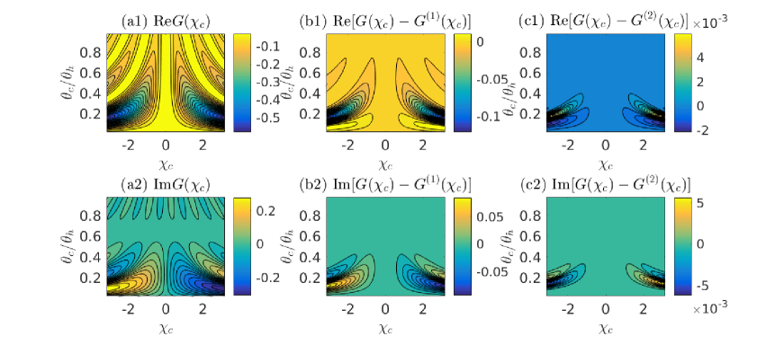
We begin our discussion by inspecting the CGF of the three-level QAR. We recall that the first-order partial CGF provides an exact result for the first cumulant (mean current), while the second-order CGF administers exact results for the first two cumulants. It is interesting to test whether these partial CGFs can further hand over reasonable estimates for higher order cumulants. In panel (a) of Fig. 2 we plot the complete CGF, $G(\chi_{c})$, obtained numerically by solving the eigenvalue problem. To present our results, we set $\chi_{w}=0$ and vary $\chi_{c}$ between $\pm\pi$. We separately display the real part of the CGF, which is even in $\chi_{c}$, and the imaginary part, which is odd in $\chi_{c}$.

We found (not shown) that the first- and second-order partial CGFs essentially look the same as the complete CGF to the naked eye. Therefore, to expose errors associated with partial CGFs we display the deviation of partial CGFs from the complete function, see panels (b) and (c). As expected, around $\chi_{c}=0$, or more precisely, when $\chi_{c}/(2\pi)\ll 1$, the partial CGFs match the exact CGF. Beyond that, deviations of the order of 20% are exhibited for $G^{(1)}(\chi_{c})$ when $\chi_{c}$ is large. The second order function $G^{(2)}(\chi_{c})$ is quite accurate even for large $\chi_{c}$, and the error stays below 0.5% throughout.

Overall, we conclude that the second-order partial CGF not only provides an exact solution for the first two cumulants, but it further prepares an excellent approximation to higher order cumulants (skewness and beyond). It should be noted that the cooling window for the presented parameters satisfies $\theta_{c}/\theta_{h}\leq 0.625$. Interestingly, the deviation of the partial CGF from the exact one, as displayed in panels (b)-(c), is most significant inside the cooling window around $\theta_{c}/\theta_{h}=0.2$.

IV.2 Performance Measures

The performance of the QAR can be optimized with respect to different observables: current, cooling efficiency, noise. As well, the thermodynamic uncertainty relation (29) connects current fluctuations with the thermodynamic cost (dissipation).

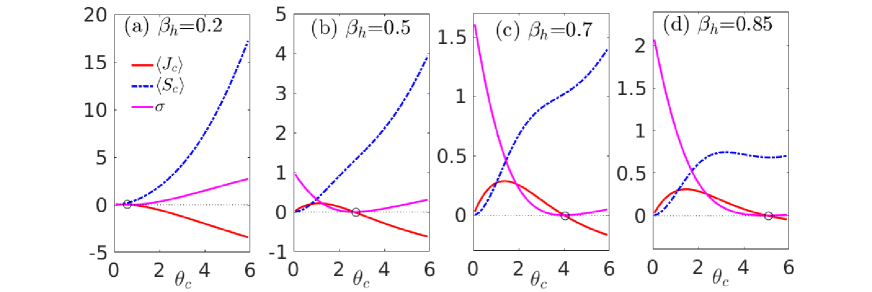
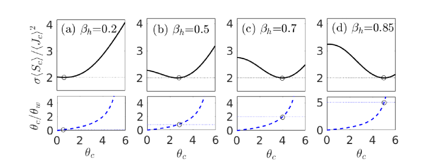
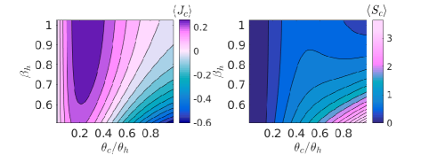
In Figs. 3-4 we exemplify the behavior of these quantities, displayed as a function of $\theta_{c}$, while tuning the temperature of the hot bath from high, $T_{w}>T_{h}\gg T_{c}$, to low, $T_{w}\gg T_{h}>T_{c}$. The system acts as a chiller when $\langle J_{c}\rangle>0$, which is the case for small enough $\theta_{c}$. It crosses into a no-cooling region outside the window of Eq. (20). In Figs. 3-4 we present results inside and outside the cooling regime so as to provide a complete picture over the behavior of current and noise in the QAR.

We circle the reversible point at which $\langle J_{\nu}\rangle=0$, the entropy production vanishes, the Carnot COP is achieved (dotted line in Fig. 4), and the TUR approaches the bound, which is nothing but the Green-Kubo relation. Away from the reversible point the entropy production rate is finite, the noise may be increased or reduced, yet overall the TUR is satisfied, as expected for a Markov process. In Fig. 4, the dashed line depicts the cooling COP, $\eta=\theta_{c}/\theta_{w}$. When $\theta_{c}/\theta_{w}$ exceeds $\eta_{c}$, the system ceases to cool, see Fig. 3. Specifically, when $\beta_{h}\to\beta_{w}$ (panel (a) of Figs. 3-4) the system operates as a chiller only at very small values for $\theta_{c}$. In this regime $\langle S_{c}\rangle$ grows monotonically. As we reduce $T_{h}$ towards $T_{c}$, panels (b)-(d) display a nontrivial behavior for the current noise: upon approaching the maximal efficiency, when the cooling current diminishes to zero, the noise may be reduced as well, see panel (d). Altogether, Figs. 3-4 present key quantities that should be considered for the optimization of cooling devices: the cooling current, its noise, dissipation, and the coefficient of performance.

The non-monotonic behavior of the current and its noise are further exemplified in Fig. 5, where we scan over $\theta_{c}$ and $\beta_{h}$. We verified numerically that these two cumulants, which were obtained from Eq. (25), exactly match the solution of the complete CGF, where we receive the cumulants by performing numerical derivatives.

IV.3 Limits and Bounds

So far, we examined the behavior of the cooling current and its noise in particular cases. Moving beyond examples, we would like to understand the behavior of the current and its noise in typical operational limits. Some of the questions that we ask are: What is the maximal cooling current, or the minimal noise that may be observed in the three-level QAR? Are there bounds on the noise or the Fano factor, defined here as a dimensionless parameter, $F\equiv\frac{\langle S_{c}\rangle}{\theta_{c}\langle J_{c}\rangle}$? Can the current and its noise expose the quantumness of the device? As we demonstrate next, indeed the first two cumulants reflect on the quantumness of the network—presented in this model through the quantum statistics of the reservoirs.

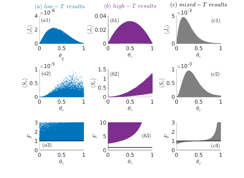
The expressions for the current and noise are quite cumbersome, and it is difficult to analytically resolve limits and bounds for performance. Let us instead numerically construct many different QAR configurations. All setups take the same total gap $\theta_{h}$, but they differ in the frequency $\theta_{c}$ and the temperatures $T_{\nu}$ while satisfying (for simplicity) $T_{c}=T_{h}<T_{w}$. The current, noise and the Fano factor of this ensemble of machines are presented in Fig. 6. Every point corresponds to a particular setup with its own combination of temperatures and frequency $\theta_{c}$, while extracting energy from the $c$ bath. Note that for simplicity we set $\theta_{h}=1$. The parameters are sampled from a uniform distribution. In panel (a), $T_{\nu}\ll\theta_{h}$; in panel (b), the reservoirs’ temperatures are high, $T_{\nu}>\theta_{h}$; in panel (c) we study the mixed scenario with $T_{w}>\theta_{h}>T_{c}$, $T_{c}=T_{h}$.

Fig. 6 shows rich characteristics; the current and noise display distinctive features in the three regimes of high-$T$, low-$T$, and mixed-$T$: (i) The current is maximized at different values for $\theta_{c}$, and it is bounded by different functional forms. (ii) Similarly, the noise behaves differently in the three cases. (iii) $F\geq 1$ in the quantum limit, $F>1$ in the classical case, but $F$ may receive values below unity in the mixed case.

It is intriguing to try and resolve the distinctive functional forms analytically. Specifically, it is evident from panel (b1) that in the classical high-$T$ regime, $\langle J_{c}\rangle\leq C\theta_{c}(\theta_{h}-\theta_{c})$, with $C$ as a constant. Studying the cooling current (18) at high temperatures by making the substitution $n_{\alpha}(\theta_{\alpha})\to T_{\alpha}/\theta_{\alpha}$, we get

$$\langle J_{c}\rangle=T_{c}\theta_{c}\frac{(T_{w}-T_{c}-\theta_{c})(\theta_{h}-\theta_{c})}{3T_{c}(2T_{w}+T_{c}+\theta_{w})+\theta_{c}(2T_{c}+T_{w}+\theta_{h}+\theta_{w})+\theta_{h}(2T_{c}+T_{w})}.$$ (30)

This relation allows us to upper bound the current,

$$\langle J_{c}\rangle<\theta_{c}(\theta_{h}-\theta_{c})\frac{(T_{w}-T_{c}-\theta_{c})}{6T_{w}}.$$ (31)

Furthermore, if $(T_{w}-T_{c})>\theta_{c}$, the function $\langle J_{c}\rangle\propto\theta_{c}(\theta_{h}-\theta_{c})$ bounds the current, in agreement with numerical simulations. This function takes a maximal value when $\theta_{c}=\theta_{h}/2$ as we clearly observe in panel (b1). The noise in panel (b2) is lower- and upper-bounded, $A\leq\frac{\langle S_{c}\rangle}{\theta_{c}^{2}}\leq B$. Based on numerical simulations we found that $A\propto T_{c}$, while $B$ corresponds to the highest temperature, $B\propto T_{w}$.

At low temperatures our numerical simulations demonstrate that the maximal current is achieved at $\theta_{c}\approx\theta_{h}/3$, while in the mixed case it is arrived at $\theta_{c}\approx 0.15\theta_{h}$. The noise $\langle S_{c}\rangle$ further displays distinctive features in the three different regimes. Altogether, Fig. 6 exposes that the ensembles of classical, quantum and mixed chillers follow different operation bounds.

The three-level QAR examined in this work does not rely on internal quantum features. The setup is referred to as “quantum” given the discreteness of the working fluid (three level system), and the quantum statistics employed for the reservoirs (Bose-Einstein distribution). Moving forward, we envisage that the survival of steady-state coherences in more complex models KilgourD may be exhibited within their noise characteristics.

V Summary

We described a full counting statistics formalism for the calculation of the cooling current and its noise in a QAR model weakly coupled to three thermal reservoirs. Achieving a closed-form analytical expression for the CGF is generally a formidable (or impossible) task for multilevel machines. However, the first two cumulants can be correctly derived by truncating the characteristic polynomial and working with a quadratic equation. While we assumed the dynamics to follow a Markovian, weak-coupling, secular quantum master equation, the procedure outlined here could be used within more sophisticated frameworks such as the nonequilibrium polaron-transformed Redfield equation Cao1 ; Cao2 . With the recent manifestations of a single-atom heat engine singleatom and a three-ion QAR QARE , measurements of current fluctuations in nanoscale machines are conceivable.

Partial CGFs could be analogously constructed to treat charge transport problems in electronic conductors and photovoltaics devices Antti1 ; Belzig ; Novotny ; Cao14 ; bijay ; Hava17 , and to examine performance bounds in biochemical reaction networks TUR1 ; Udo ; Wolde . Our work here was focused on the zero-frequency current noise. Partial CGF could be similarly used to obtain the full spectrum of the noise in multi-level systems junjie . Future work will be dedicated to the investigation of noise and efficiency bounds in multilevel refrigerators where quantum coherences play a role KilgourD , and to the study of performance bounds under strong system-bath coupling effects.