Converting non-relativistic dark matter to radiation

Abstract

Dark matter in the cosmological concordance model is parameterised by a single number, describing the covariantly conserved energy density of a non-relativistic fluid. Here we test this assumption in a model-independent and conservative way by considering the possibility that, at any point during the cosmological evolution, dark matter may be converted into a non-interacting form of radiation. This scenario encompasses, but is more general than, the cases where dark matter decays or annihilates into these states. We show that observations of the cosmic microwave background allow to strongly constrain this scenario for any conversion time after big bang nucleosynthesis. We discuss in detail, both from a Bayesian and frequentist point of view, in which sense adding large-scale structure observations may even provide a certain preference for a conversion of dark matter to radiation at late times. Finally we apply our general results to a specific particle physics realisation of such a scenario, featuring late kinetic decoupling and Sommerfeld-enhanced dark matter annihilation. We identify a small part of parameter space that both mitigates the tension between cosmic microwave and large-scale structure data and allows for velocity-dependent dark matter self-interactions strong enough to address the small-scale problems of structure formation.

I Introduction

There is overwhelming evidence for the existence of dark matter (DM) in our Universe from various astrophysical and cosmological observations. While many of its particle physics properties are completely unknown, the amount of DM at the time of recombination has been precisely determined through observations of the Cosmic Microwave Background (CMB) Ade et al. (2016a). The corresponding DM relic abundance is typically assumed to have been set early on, at temperatures comparable to the DM mass in the most commonly considered scenario of thermally produced DM particles Lee and Weinberg (1977); Gondolo and Gelmini (1991), such that the comoving DM density is constant throughout the subsequent cosmological evolution.

In this work we analyse how cosmological observations constrain deviations from the simple picture of a comovingly constant DM density. An interesting example for a possible underlying mechanism is if all or a part of the DM is unstable. If the decay products are Standard Model (SM) states such as electrons or photons, a scenario of this type will be strongly constrained by a variety of cosmological and astrophysical probes (see e.g. Cirelli et al. (2012); Ibarra et al. (2013); Poulin et al. (2017)). It is however an interesting possibility that the decay products are new massless or very light states in the dark sector, such that effectively a fraction of DM is converted into relativistic ‘dark’ radiation (DR) Zentner and Walker (2002); Ichiki et al. (2004); Lattanzi and Valle (2007); Peter (2010); Wang and Zentner (2010); Bjaelde et al. (2012); Allahverdi et al. (2015); Audren et al. (2014); Poulin et al. (2016). Such a conversion has received some interest lately as it has been argued to alleviate a possible tension between measurements of the CMB and large scale structure (LSS) observables Enqvist et al. (2015); Berezhiani et al. (2015); Blackadder and Koushiappas (2016); Pourtsidou and Tram (2016); Poulin et al. (2016); Chudaykin et al. (2016); Hamaguchi et al. (2017).

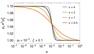
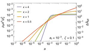
Figure 1: Left panel. Evolution of comoving DM density for the step-like transition described by Eq. (1), for a transition redshift of $a_{t}=10^{-3}$, a conversion factor of $1+\zeta=1.1$ and, as indicated, four values of the parameter $\kappa$ characterising the steepness of the transition. For comparison, we also show the case of decaying DM (dotted line), assuming that a fraction $\zeta/(1+\zeta)$ of the initial DM abundance decays with a rate $\Gamma=0.15H_{\rm eq}$. Right panel. Resulting evolution of the comoving DR density as given in Eq. (5). This assumes that there is no additional (e.g. constant) source of DR and, for the translation to $\Delta\tilde{N}_{\rm eff}$ as defined in Eq. (6), we have here chosen $\rho_{\chi}^{0}$ to agree with the value of $\Omega_{\chi}^{0}h^{2}=0.1198$ measured by Planck.

A second example in which the comoving dark matter density can change is if the DM annihilation rate becomes relevant at late times, which may happen if the annihilations experience a sufficiently strong Sommerfeld enhancement Dent et al. (2010); Zavala et al. (2010); Feng et al. (2010); van den Aarssen et al. (2012a); Armendariz-Picon and Neelakanta (2012); Binder et al. (2018). Yet another case where DM may be converted into DR is given by merging primordial black holes emitting gravitational waves Nakamura et al. (1997); Raidal et al. (2017), a scenario currently receiving a lot of interest due to the observations by advanced LIGO Abbott et al. (2016). We note that also ordinary astrophysical processes can convert matter into radiation, but only at rates below the sensitivity of (near) future observation Camarena and Marra (2016).

In this work we employ data from the CMB as well as LSS observables to constrain the possibility of DM being converted into DR in a model-independent way. Clearly the amount of DM which is allowed to be converted into DR will depend on the time of this conversion, given that the relative contributions of matter and radiation to the overall energy density change as the Universe evolves. Also the rate of this conversion is expected to have an impact on the constraints. We will concentrate on conversion times well after the end of primordial nucleosynthesis, as sufficiently early transitions can always be mapped onto a cosmology with a constant additional radiation component, $\Delta N_{\text{eff}}>0$.

This article is structured as follows: In the next section we will discuss how we implement the DM-DR transition. In Sec. III we will discuss the effects on the CMB as well as the resulting constraints, while Sec. IV is devoted to the discussion of low redshift observables. In Sec. V we will map our general constraints to the case of Sommerfeld enhanced annihilation, before we conclude in Sec. VI.

II Converting dark matter to dark radiation

As motivated in the introduction, our aim is to quantify in rather general terms i) how much DM can be converted to DR, as well as how this depends on the ii) time and iii) rate of this conversion. Phenomenologically we are thus interested in a step-like transition in the comoving DM density as shown in the left panel of Fig. 1 where, at least for the moment, we choose to remain completely agnostic about the underlying mechanism that causes such a transition. Nevertheless, we emphasise that the parametrisation is sufficiently general to capture a range of interesting scenarios, such as the case of a decaying DM sub-component (indicated by a black dotted line in Fig. 1) and Sommerfeld-enhanced DM annihilations. The latter case will be the subject of Sec. V, where we will discuss in detail how to map the underlying particle physics parameters onto the effective parametrisation discussed in this section.

II.1 Evolution of background densities

In the following, we will adopt a simple parametric form for the DM density $\rho_{\chi}(a)$ as shown in Fig. 1, namely

$$\rho_{\chi}(a) =\frac{\rho^{0}_{\chi}}{a^{3}}\left[1+\zeta\frac{1-a^{\kappa}}{1+(a/a_{t})^{\kappa}}\right]\,.$$ (1)

Here $a$ denotes the scale factor of the Friedman-Robertson-Walker (FRW) metric, $\rho^{0}_{\chi}\equiv\rho_{\chi}(1)$ the DM density today, and the three parameters $(\zeta,a_{t},\kappa)$ directly relate to the points i) – iii) raised above. Specifically, the comoving DM density decreases in total by a factor of $1+\zeta$, the transition is centred at $a=a_{t}$, and the parameter $\kappa$ determines how fast the transition occurs.

This parametrisation enables us in particular to understand which properties of DM-DR conversion are constrained observationally. For example, we will see below that for a conversion after recombination constraints are largely independent on when and how quickly the transition occurs, but mostly depend only on the total amount of DM converted to DR. A similar observation was previously made for the case of a sub-dominant component of DM decaying into DR Poulin et al. (2016), and our findings generalise this result. Conversely, for a very early transition, we find constraints to depend only on the total amount of DR produced, which can be described by the effective number of neutrino species $N_{\text{eff}}$. For transitions around matter-equality, on the other hand, the constraints can no longer be understood in terms of these simple limiting behaviours, and depend in a more complicated way on when and how quickly the conversion takes place.

As already stressed, the phenomenological parametrisation suggested above allows to capture a significant range of cosmologically interesting scenarios. For example, we find that the case of a decaying DM sub-component can be accurately described by setting $\kappa=2$ and choosing $a_{t}$ such that the Hubble expansion rate at the transition is comparable to the decay rate. Sommerfeld-enhanced annihilations, on the other hand, can be accurately matched by setting $\kappa=1$ (see Sec. V).

By assumption, we demand that this transition occurs because DM is being converted to radiation. The rates of change of the comoving DM and DR densities must thus be of equal size, and opposite in sign:

$$\frac{1}{a^{3}}\frac{\mathrm{d}}{\mathrm{d}t}\left(a^{3}\rho_{\chi}\right)=-\frac{1}{a^{4}}\frac{\mathrm{d}}{\mathrm{d}t}\left(a^{4}\rho_{\phi}\right)\,.$$ (2)

Alternatively, we can write this statement in terms of coupled Boltzmann equations for the two fluid components:

$$\frac{\mathrm{d}\rho_{\chi}}{\mathrm{d}t}+3H\rho_{\chi} \equiv -\mathcal{Q}$$ (3)

$$\frac{\mathrm{d}\rho_{\phi}}{\mathrm{d}t}+4H\rho_{\phi} = \mathcal{Q}\,,$$ (4)

where $H=\dot{a}/a$ is the Hubble rate and $\mathcal{Q}>0$ describes the (momentum-integrated) collision term. In this formulation, being agnostic about the underlying mechanism of the DM to DR transition simply means, as indicated, that we start from Eq. (1) and view Eq. (3) as a definition for $\mathcal{Q}$ – rather than determining $\rho_{\chi}$ from a given collision term.

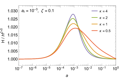
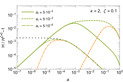
Figure 2: Left panel. Evolution of Hubble rate for the same scenarios as shown in Fig. 1, compared to the $\Lambda$CDM Hubble rate $H^{\zeta=0}$ (which in our scenarios is obtained for $\zeta=0$), Right panel. Impact of changing $a_{t}$ on the Hubble rate, for $\kappa=2$. Orange (thinner) lines indicate the impact of the produced DR alone. For the $a_{t}=5\cdot 10^{-6}$ case we show, for comparison, also how the Hubble rate is affected by a constant DR contribution, characterised by a constant $\Delta N_{\rm eff}$ (black dotted line).

We can now obtain the DR energy density by integrating Eq. (2), with the boundary condition $\rho_{\phi}(a\to 0)=0$. This leads to

$$\rho_{\phi}(a) =\zeta\frac{\rho_{\chi}^{0}}{a^{3}}\frac{\left(1+a_{t}^{\kappa}\right)}{\left(a^{\kappa}+a_{t}^{\kappa}\right)}$$ (5)

$$\times\left(\left(a^{\kappa}+a_{t}^{\kappa}\right)\,_{2}F_{1}\left[1,\frac{1}{\kappa};1+\frac{1}{\kappa};-\left(\frac{a}{a_{t}}\right)^{\kappa}\right]-a_{t}^{\kappa}\right)\,,$$

where ${}_{2}F_{1}$ denotes the ordinary Hypergeometric functions. Let us stress that the above solution for the DR energy density $\rho_{\phi}(a)$ does not explicitly depend on the form of $H$, which is one of the advantages of our parametrisation for $\rho_{\chi}(a)$. This implies that also the transition from radiation to matter domination is fully and consistently covered in this approach (at least at the level of the evolution of background densities). In the right panel of Fig. 1, we show how the DR density evolves, according to Eq. (5), for the $\rho_{\chi}(a)$ scenarios plotted in the left panel. To facilitate comparison with the literature, we also indicate the amount of DR in terms of an effective number of additional neutrino species, by defining

$$\Delta\tilde{N}_{\text{eff}}(a)\equiv\frac{\rho_{\phi}(a)}{\rho_{1\nu}(a)}=\frac{8}{7}\left(\frac{11}{4}\right)^{4/3}\frac{\rho_{\phi}(a)}{\rho_{\gamma}(a)}\;,$$ (6)

where the last equality is only valid for sufficiently late times (after $e^{\pm}$ annihilation). For $\rho_{\phi}\propto a^{-4}$, this reduces to the standard definition of the effective number of additional neutrino species, $\Delta\tilde{N}_{\text{eff}}\to\Delta{N}_{\text{eff}}$, typically used to describe a (comovingly) constant contribution of DR. In the scenarios that we describe here, the comoving DR density is not constant (but saturates for $a\gg a_{t}$ if $\kappa>1$).

We note that the large range of transition histories that we consider here essentially also includes the case of decaying DM, which much of the literature has focused on so far. To illustrate this, we include in the same figure the case of a 2-component DM model, where one component is stable and the other decays (dotted lines). To make the comparison more straight-forward for the purpose of this figure, we have adjusted the decaying component to make up a fraction $\zeta/(1+\zeta)$ of the initial DM density and tuned the decay rate $\Gamma$ such that the total DM density intersects with the other curves at $a=a_{t}$.

Let us conclude the discussion of how the DM and DR densities evolve in our transition scenarios by showing in Fig. 2 the induced effect on the expansion rate of the Universe. For the purpose of this figure, we compute the Hubble rate $H^{2}=8\pi G\rho/3$ by fixing the density parameters for the various components to the mean $\Lambda$CDM values resulting from the Planck TTTEEE+lowP analysis Ade et al. (2016a), taking $\Omega_{\chi}^{0}h^{2}=0.1198$ to correspond to the DM density today, and compare it to the Hubble rate in the $\Lambda$CDM case that is obtained for $\zeta\to 0$. During radiation domination, as seen in the left panel, the Hubble rate starts to be visibly affected as soon as the additional comoving DM density compared to its value today, $\zeta\rho_{\chi}^{0}$, contributes sufficiently to the total energy density; for the small values of $\zeta$ shown here, this happens not much earlier than the transition at $a=a_{t}$. The largest deviation of the Hubble rate occurs at $a\sim a_{t}$ during matter domination, or somewhat earlier during radiation domination (right panel). As indicated by the thin orange lines, furthermore, the DR density always starts to change the Hubble rate only at later times; as expected, its relative impact (compared to that of DM), is largest if the transition takes place during radiation domination (and then, for $\kappa=2$ and $\kappa=4$, mimics the impact of a constant $\Delta N_{\rm eff}$ after equality, cf. the black dotted line).

II.2 Perturbations

In order to study the impact of our modified cosmological scenario on CMB and LSS observables, we must not only account for the modified evolution of the background densities, but also include the effect of perturbations. In synchronous gauge Ma and Bertschinger (1995), the perturbed line element of the FRW metric is given by

$$\mathrm{d}s^{2} =g_{\mu\nu}\mathrm{d}x^{\mu}\mathrm{d}x^{\nu}=a^{2}\left[-\mathrm{d}\tau^{2}+(\delta_{ij}+h_{ij})\mathrm{d}x^{i}\mathrm{d}x^{j}\right]\,,$$ (7)

where $\tau$ is the conformal time and $h_{ij}$ are the metric perturbations (we will denote its trace as $h\equiv h_{ii}$).

The above form of the line element leaves a residual gauge freedom, which we remove by working in comoving synchronous gauge (as also used, e.g., in CAMB Lewis et al. (2000); Howlett et al. (2012)). In this gauge, the DM fluid remains at rest and its four-velocity is thus given by $u^{\chi}_{\,\mu}=a\,(1,\mathbf{0})$ just as in the unperturbed case. The full DM and DR energy momentum tensors are then of the form

$$T^{\chi}_{\mu\nu} =\rho_{\chi}u^{\chi}_{\mu}u^{\chi}_{\nu}\,,$$ (8)

$$T^{\phi}_{\mu\nu} =\frac{4}{3}\rho_{\phi}u^{\phi}_{\mu}u^{\phi}_{\nu}+\frac{\rho_{\phi}}{3}g_{\mu\nu}+\Pi_{\mu\nu}^{\phi}\,,$$ (9)

where $u^{\phi}_{\,\mu}=a\,(1,\mathbf{v^{\phi}})$ denotes the DR four-velocity, and $\rho_{\chi}$ and $\rho_{\phi}$ now refer to the full (perturbed) energy densities. $\Pi_{\mu\nu}^{\phi}$ describes the anisotropic stress of the DR component, i.e. perturbations away from the perfect fluid form (as, e.g., caused by free-streaming).

As before, we demand that any decrease in DM is fully compensated by an increase in DR. Covariant conservation of energy thus implies $\nabla^{\nu}\left(T^{\chi}_{\mu\nu}+T^{\phi}_{\mu\nu}\right)=0$, which we can formally split and rewrite as

$$\nabla^{\nu}T^{\chi}_{\mu\nu}=-\nabla^{\nu}T^{\phi}_{\mu\nu}\equiv-\mathcal{Q}u^{\chi}_{\mu}\,,$$ (10)

where $\nabla^{\mu}$ denotes the covariant derivative with respect to the full (perturbed) metric $g_{\mu\nu}$ given in Eq. (7). To leading order, as expected, this simply reproduces Eqs. (2–4). Demanding the DM density to evolve as in Eq. (1) thus provides the same definition of $\mathcal{Q}\propto\zeta$ at leading order.

At next order in the perturbed quantities, the DM part of Eq. (10) becomes

$$\delta^{\prime}_{\chi}+\frac{1}{2}h^{\prime}=\frac{a}{\rho_{\chi}}\left(\mathcal{Q}\delta_{\chi}-\delta\mathcal{Q}\right)\,.$$ (11)

Here, the prime ^′ denotes a derivative with respect to conformal time and $\delta_{\chi}=\delta\rho_{\chi}/\rho_{\chi}$ is the usual dimensionless perturbation in the DM density. The perturbation $\delta\mathcal{Q}$ to $\mathcal{Q}$ would, in analogy to the leading order result, be defined by an extension of our ansatz in Eq. (1) to include perturbations. The minimal option for such an extension, in some sense, is that the perturbations only affect the volume expansion (and hence not the comoving DM density). In other words, one would have to replace only the leading factor in Eq. (1),

$$\rho_{\chi}=\frac{\rho^{0}_{\chi}}{(a+ah/6)^{3}}\left[1+\zeta\frac{1-a^{\kappa}}{1+(a/a_{t})^{\kappa}}\right]\,.$$ (12)

Such an ansatz for the DM density implies $\delta^{\prime}_{\chi}=-\frac{1}{2}h^{\prime}$, as can easily be verified, and is hence equivalent to setting

$$\delta\mathcal{Q}\equiv\mathcal{Q}\delta_{\chi}\,.$$ (13)

While we will adopt this choice in the following, for simplicity, we stress that it is model-dependent and a full discussion is beyond the scope of this work. We will, however, get explicitly back to this issue in Section V when we try to motivate $\mathcal{Q}$ from the collision term in the Boltzmann equation for a specific scenario (rather than by directly postulating the evolution of the DM density). In general, it is worth noting that any deviation from Eq. (13) must be proportional to $\mathcal{Q}$ which, as we will see, is strongly constrained already from the evolution of the background densities (unless $a_{t}$ is very small – in which case the scale of the horizon, and hence of any perturbation that can be affected, is much smaller than what can be probed by the CMB). For the case of decaying DM, furthermore, Eq. (13) is exactly satisfied Poulin et al. (2016).

To first order in the perturbed quantities related to DR, on the other hand, Eq. (10) takes the form

$$\delta^{\prime}_{\phi}+\frac{2}{3}h^{\prime}+\frac{4}{3}\theta_{\phi} =-\frac{a}{\rho_{\phi}}\left(\mathcal{Q}\delta_{\phi}-\delta\mathcal{Q}\right)\,,$$ (14)

$$\theta^{\prime}_{\phi}+\frac{1}{4}\nabla^{2}\delta_{\phi}+\frac{1}{2\rho_{\phi}}\nabla^{4}\Pi^{\phi} =-\frac{a}{\rho_{\phi}}\mathcal{Q}\theta_{\phi}\,.$$ (15)

Here, $\nabla^{2}$ is the Laplacian operator, $\delta_{\phi}\equiv\delta\rho_{\phi}/\rho_{\phi}$ is defined in analogy to the DM case, and $\theta_{\phi}\equiv\partial_{i}v_{\phi}^{i}$ is the scalar part of the DR velocity. In the second equation, we have as usual only considered the scalar part of $\nabla^{\nu}T^{\phi}_{i\nu}$, by taking its divergence, because the vector part of the perturbations only have decaying modes. This is the reason why only the scalar part of the anisotropic stress enters, defined as $\Pi_{ij}^{\phi,\text{scalar}}\equiv\left(\partial_{i}\partial_{j}-\frac{1}{3}\delta_{ij}\nabla^{2}\right)\Pi^{\phi}$. We implement this part as for an additional neutrino species, where $\Pi^{\phi}$ arises due to the effect of free-streaming Weinberg (2004).

Let us point out that for $\mathcal{Q}=0$ Eqs. (14,15) simply describe the standard way of including non-interacting relativistic degrees of freedom, e.g. in the form of (sterile) neutrinos, and for the choice of $\delta\mathcal{Q}$ made in Eq. (13) we recover exactly the case of decaying dark matter (assuming an appropriate choice of $\mathcal{Q}$, cf. Fig. 1). We re-iterate that we expect a small effect from including perturbations because $\mathcal{Q}$ (and hence $\delta Q$) is already strongly constrained from the evolution of the background densities.

III Generic effects on the cosmic microwave background

III.1 Changes in the temperature anisotropy spectrum

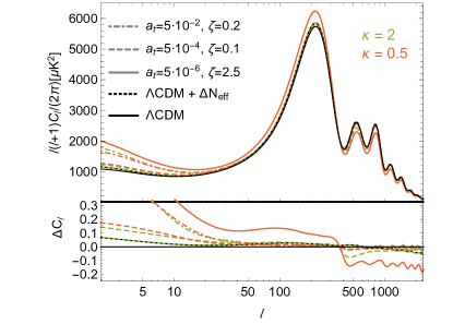
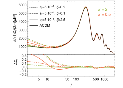
Figure 3: Lensed TT spectra for transition rates of $\kappa=2$ (green) and $\kappa=1/2$ (orange) for three different transition times $a_{t}=5\cdot 10^{-6}$, $5\cdot 10^{-4}$, $5\cdot 10^{-2}$ for fixed $\Lambda$CDM parameters (left) and for the respective best-fit points (right). For comparison we show the $\Lambda$CDM spectrum (solid black line) as well as $\Lambda$CDM $+\Delta N_{\text{eff}}$ (dashed black line) for comparison with the early transition case. In the bottom panels we show the fractional difference between the different scenarios and the $\Lambda$CDM case. See text for the remaining parameter values of the models used to obtain these spectra.

The spectrum of the CMB is sensitive to the amount of matter and radiation from time-scales starting at around recombination until late times (e.g. through lensing effects). In addition, even earlier epochs may be constrained if they leave an imprint at later times such as an extra DR component. Let us start the discussion of CMB constraints by an evaluation of the possible imprints of the scenario described in Sec. II on the CMB spectrum.

The $\Lambda$CDM model is described by only six parameters, which may be chosen as i) the amount of baryons $\Omega_{b}h^{2}$ and ii) dark matter $\Omega_{\chi}h^{2}$, the iii) approximate angular size of the sound horizon $\theta_{\text{MC}}$, the iv) re-ionisation optical depth $\tau$, the v) amplitude of scalar perturbations $\ln(10^{10}A_{s})$ and the vi) scalar spectral index $n_{s}$. Given that the $\Lambda$CDM cosmology provides an excellent fit to the CMB data, any deviations should be very tightly constrained.

To calculate CMB as well as LSS observables, we use a modified version of the publicly available Boltzmann code CAMB Lewis et al. (2000); Howlett et al. (2012). In particular we have implemented the non-standard time evolution of energy densities of DM and DR according to Eqs. (1) and (5) to investigate and constrain the imprints of our scenario on the CMB. As described in Section II.2, furthermore, we treat DR as an extra neutrino species.

As discussed in the last section, the qualitative features of the DM to DR conversion depend on the time $a_{t}$ as well as the rate $\kappa$ of the conversion. To capture the relevant effects for the different regimes, we consider three different transition times $a_{t}=5\cdot 10^{-6},5\cdot 10^{-4}$ and $5\cdot 10^{-2}$ as well as two different conversion rates $\kappa=2$ and ${1}/{2}$. The transition times are chosen such that we cover radiation domination as well as matter domination before and after recombination, while the choices of $\kappa$ describe, respectively, a fast and a slow conversion scenario.

To illustrate the effect on the CMB spectrum we fix five of the six $\Lambda$CDM parameters to their Planck 2015 TTTEEE +low-P Ade et al. (2016a) mean values, i.e., $\Omega_{b}h^{2}=0.02225$, $100\theta_{\text{MC}}=1.04077$ , $\tau=0.0790$, $\ln(10^{10}A_{s})=3.094$ and $n_{s}=0.9645$. The DM density is naturally evolving within our scenario and we fix $\Omega_{\chi}h^{2}$ such that for any $\kappa$, $\zeta$ and $a_{t}$ we have $\Omega_{\chi}h^{2}=\Omega_{\chi}h^{2}|_{\Lambda\text{CDM}}$ at $z_{\text{rec}}\equiv 1100$, i.e. we require the same amount of DM as inferred for the $\Lambda$CDM model around recombination. This choice essentially ensures that the first peak of the CMB spectrum resembles that of the $\Lambda$CDM model and therefore agrees well with observations. We show the TT spectra of our scenario as well as the fractional difference from the usual $\Lambda$CDM paradigm, with parameters fixed in the way just described, in the left panel of Fig. 3. In the right panel of Fig. 3, for comparison, we show the spectra for the same values of our model parameters ($\kappa$, $a_{t}$, $\zeta$), but with the $\Lambda$CDM parameters fixed to the respective best-fit values in these scenarios.

Let us begin our discussion with a couple of simple observations: For a rather quick transition $(\kappa=2$) which happens rather early $(a_{t}=5\cdot 10^{-6})$, the transition will be complete before the onset of matter domination and thus the only significant change compared to the $\Lambda$CDM case is due to a remaining extra component of DR from the conversion. Given that the conversion takes place during radiation domination where the DM energy density is sub-leading, rather large values of $\zeta$ are consistent with data (for the chosen value of $\zeta=2.5$ we obtain $\Delta\tilde{N}_{\text{eff}}(1)\simeq 0.42$). Once the conversion is complete the comoving energy density of DR will remain constant. We thus expect this model to have a spectrum which is very similar to the $\Lambda$CDM case with a constant additional $\Delta N_{\text{eff}}=0.42$. We illustrate this case with a dashed black line in the plot. As expected the spectrum is almost identical, and only very small differences are visible for high values of $\ell$, which are most sensitive to early times. We have confirmed that for even earlier transition times the two cases are indistinguishable. For a very slow transition $(\kappa=0.5)$ on the other hand, a significant part of the matter density will be converted to radiation much later, implying that a larger fraction of the initial matter density will end up in radiation such that the effect on the CMB will be significantly larger, which can also clearly be seen in Fig. 3. We therefore expect this case to be much more strongly constrained. For very late transitions, $(a_{t}=5\cdot 10^{-2})$, the cosmic history is the same as for the $\Lambda$CDM case until recombination. We accordingly observe that the spectrum resembles the $\Lambda$CDM case for high multipoles as expected.

A more detailed understanding of the different effects on the power spectra requires knowledge about the evolution of the different energy densities $\Omega_{i}$. Given that we fix the value of $\Omega_{\chi}h^{2}=\Omega_{\chi}h^{2}|_{\Lambda\text{CDM}}$ at $z=z_{\text{rec}}$ (for the left panel in Fig. 3) while having at the same time a somewhat increased value of $h$ due to the extra radiation component, $\Omega_{\chi}$ will be correspondingly smaller. Requiring the Universe to remain flat, $\sum\Omega_{i}=1$, the energy density within some other components needs to be increased to compensate the decrease in $\Omega_{\chi}$. The way in which the different components change depends on which parameters we keep fixed in the analysis. For instance fixing $\theta_{\text{MC}}$ as we have done in the left panel of Fig. 3 will lead to an enhancement in $\Omega_{\Lambda}$, because the enhancement of the Hubble rate prior to recombination decreases the size of the sound horizon at the surface of last scattering $r_{s}$, which implies a simultaneous decrease of the angular distance to the last scattering surface $D_{A}$ in order to keep $\theta_{\text{MC}}$ fixed. The required decrease in $D_{A}$ in turn is achieved by increasing the vacuum energy $\Omega_{\Lambda}$. Overall this will lead to an enhanced Late time Integrated Sachs Wolfe (LISW) effect, that is (relatively speaking) more power on very large scales (small values of $\ell$).

As these types of effects strongly depend on what we keep fixed, we will refrain from describing the changes of the temperature anisotropies compared to the $\Lambda$CDM case in more detail. To construct the bounds on the model parameters in the next section, all $\Lambda$CDM parameters will be varied, allowing for a partial compensation of the effects of the matter to radiation transition. This partial compensation can already be anticipated by comparing the left and right panels of Fig. 3.

III.2 CMB constraints

In this section, we will constrain our model with CMB observations. The concrete data set that we use for this purpose, with likelihoods as implemented in the publicly available Markov Chain Monte-Carlo (MCMC) code CosmoMC Lewis and Bridle (2002); Lewis (2013), we will denote as follows:

• CMB: Planck TTTEEE + lowTEB Aghanim et al. (2016)

At this stage, in particular, we do not add information from the Planck lensing power spectrum reconstruction Ade et al. (2016b) because this effectively adds a measurement implicitly related to the matter power spectrum (which we will discuss in more detail in the next section).

In order to explore the parameter space of our model, we modify CosmoMC to communicate our additional model parameters to the modified CAMB version described above. We run chains using the fast/slow sampling method Neal (2005); Lewis (2013), as recommended for a large parameter space. We assume the chains to be converged if the Gelman-Rubin criterion ($R$) Gelman and Rubin (1992) satisfies $R-1<0.01$. Along with a large number of Planck nuisance parameters, we scan over the six $\Lambda$CDM parameters with flat priors as follows:

$$\Omega_{b}h^{2}\in(0.01,0.1),~{} \Omega_{\chi}^{0}h^{2}\in(0.01,0.5)$$

$$100\theta_{\rm MC}\in(0.8,2),~{} \tau\in(0.01,0.2)$$

$$\ln(10^{10}A_{s})\in(2,4),~{} ~{}n_{s}\in(0.8,1.2)\,.$$ (16)

Let us first have a look at very early transitions. In this case, as discussed above, CMB constraints on our model should be equivalent to those for a model with constant $\Delta N_{\text{eff}}$ (at least for large values of $\kappa$, since for $\kappa\leq 1$ the comoving DR energy density does not saturate, cf. Fig. 1). To check this expectation, we fix $a_{t}=10^{-7}$ and scan over the six $\Lambda$CDM parameters and $\zeta\geq 0$ (with a flat prior). For comparison with the constant $\Delta N_{\text{eff}}$ case, we use the default CosmoMC/CAMB implementation with $N_{\rm eff}$ as a free parameter in addition to the $\Lambda$CDM parameters. For this scan we have set the (flat) prior for $N_{\rm eff}$ to be greater than 3.046, in order to be comparable to the prior choice for our model parameter $\zeta$.

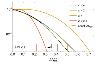
Figure 4: Marginalised 1D posterior pdfs for $\Delta\tilde{N}_{\text{eff}}(a_{\text{rec}})$, normalised such that the maximum value is 1, using the CMB dataset only. The solid lines are for $\kappa=0.5,1,2,4$ with fixed $a_{t}=10^{-7}$. Note that for $\kappa=2,4$, but not for smaller values of $\kappa$, we have $\Delta\tilde{N}_{\text{eff}}(a_{\text{rec}})=\Delta\tilde{N}_{\text{eff}}^{\rm today}$, cf. Fig. 1. For comparison, we also include the standard case of a constant $\Delta N_{\text{eff}}\geq 0$ (dashed black line). The vertical lines indicate the corresponding 95% C.L. limits. For a constant $\Delta N_{\text{eff}}$, our limit is in good agreement with the Planck limit of $0.35$ Ade et al. (2016a) (obtained with a flat prior on $\Delta N_{\rm eff}$ that, unlike in our case, also allows $\Delta N_{\rm eff}<0$).

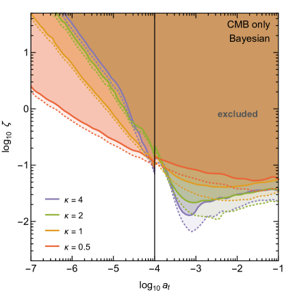
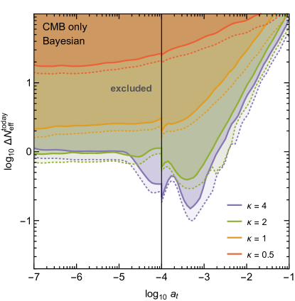
Figure 5: 95% C.L. (dotted lines) and 99% C.L. (solid lines) Bayesian limits from CMB only; the coloured region above each line is excluded. Left panel. Constraints on the amount of converted DM, cf. Eq. (1). Right panel. Constraints on the amount of DR today, expressed in terms of $\Delta\tilde{N}_{\rm eff}$ as given in Eq. (6). For both cases, we adopted a flat prior on $\Delta N_{\rm eff}^{\rm today}$ for $a_{t}<10^{-4}$, and a flat prior on $\zeta$ for $a_{t}>10^{-4}$.

In Fig. 4, we show the marginalised 1D posterior probability density functions (pdfs) for $\Delta\tilde{N}_{\rm eff}(a_{\text{rec}})$ that result from the CMB likelihood, for $\kappa=0.5,1,2,4$. For $\kappa=2,4$, the posteriors are indeed similar to the case of a constant $\Delta N_{\text{eff}}$ (shown as a black dashed line). The discrepancy at larger values of $\Delta\tilde{N}_{\rm eff}(a_{\text{rec}})$ can be traced back to how the Helium abundance $Y_{\rm He}$ enters in the CMB code. Concretely, $Y_{\rm He}$ is a derived parameter that depends not only on the baryon density but also on the DR density at the time of big bang nucleosynthesis (BBN), because a non-zero value of the latter affects the Hubble expansion rate during that time Peebles (1966); Hou et al. (2013). In our case, unlike for a constant $\Delta N_{\text{eff}}$, there is no DR present during BBN because we always assume that the DM to DR transition occurs only much later. We checked explicitly that we get exact agreement between our $\kappa=2,4$ limits and constant $\Delta N_{\text{eff}}$, up to 99 % C.L., if we use a numerical value of $Y_{\rm He}$ as calculated from $\Delta\tilde{N}_{\rm eff}({\text{BBN}})=\Delta\tilde{N}_{\rm eff}({\text{today}})$. Lastly, let us mention that these limits also agree to a good approximation with the Planck limits on a constant $N_{\rm eff}$ Ade et al. (2016a) – though such a comparison should be taken with a grain of salt given that those limits are based on a slightly different prior choice (allowing for $\Delta N_{\rm eff}<0$) than what we have adopted here.

We now turn to the CMB constraints when scanning freely over our model parameters. For this, we choose a flat prior on $\log a_{t}$, constraining the scan to $-7\leq\log_{10}a_{t}\leq-1$ in order to focus on the case where BBN constraints are negligible (lower bound) and to ensure that we can neglect the effect of structure formation and still treat the perturbations at the linear level (upper bound). We note that the upper bound here is somewhat optimistic in this respect, so results presented for $a_{t}\gtrsim 10^{-2}$ should be interpreted with care (what actually matters is of course not the value of $a_{t}$, but whether the transition is largely completed while perturbations still are at the linear level, cf. Fig. 1). For $\zeta$ we choose a more complicated prior to optimise the sampling efficiency of the Metropolis-Hastings algorithm implemented in CosmoMC. Concretely, in anticipation of our results, we choose a prior for $\zeta$ that corresponds to a flat prior on $\Delta N_{\rm eff}^{\rm today}$ for $a_{t}<10^{-4}$ and a prior that is flat in $\zeta$ itself for $a_{t}>10^{-4}$. Since for fixed $a_{t}$ and fixed cosmological parameters $\Delta N_{\rm eff}^{\rm today}$ is directly proportional to $\zeta$, the two regions are expected to smoothly connect to each other at $a_{t}=10^{-4}$.

We show our results in Fig. 5, as a function of $a_{t}$, both expressed in terms of limits on $\log_{10}\zeta$ (left panel) and in terms of limits on $\log_{10}\Delta\tilde{N}_{\rm eff}$ today (right panel). For the sake of our later discussion, let us stress that these are Bayesian limits constructed in the standard way, i.e. curves of constant 2D (marginalised) posterior probabilities chosen such that the integral over the enclosed area (which includes the point of maximum pdf) results in 0.95 and 0.99, respectively. For very small values of $a_{t}$, as discussed above, we expect that the CMB cannot distinguish between our model and the case of a constant $\Delta N_{\rm eff}$. This implies that the bound on $\zeta$, as a function of $a_{t}$, must simply be inversely proportional to the total amount of DR that is created prior to recombination. For a fast transition ($\kappa=2$ and $\kappa=4$) the latter is roughly proportional to the ratio of the amount of converted DM to the total amount of radiation, which in turn is proportional to $\zeta\,a_{t}$. This explains the approximate $\zeta\propto a_{t}^{-1}$ slope visible in the figure.

Closer inspection reveals that the simple requirement of a fixed total amount of DR just before recombination indeed gives a qualitatively very good description of the limits for $a_{t}\lesssim 10^{-3}$. We note that the limits in this range can also be reproduced, within reasonable accuracy, just by using the fact that the CMB peak positions are tightly constrained observationally. For large values of $a_{t}$, on the other hand, the constraints are less and less affected by the additional radiation component and rather driven by the reduced CDM component – which explains why the maximally allowed value of $\zeta$ becomes almost independent of $a_{t}$ at very late times. Physically, it is a combination of various mechanisms that sets the constraints in this case, with the ISW effect becoming more and more relevant with increasing $a_{t}$. While we refrain from attempting a detailed discussion here, we therefore expect that simple prescriptions for estimating these constraints are likely to fail. For example, demanding the peak positions not to change (which gave a very good estimate of the full results for $a_{t}\lesssim 10^{-3}$) would result in constraints that are too strong and feature a qualitatively wrong dependence on $a_{t}$.

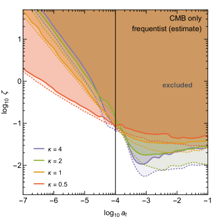
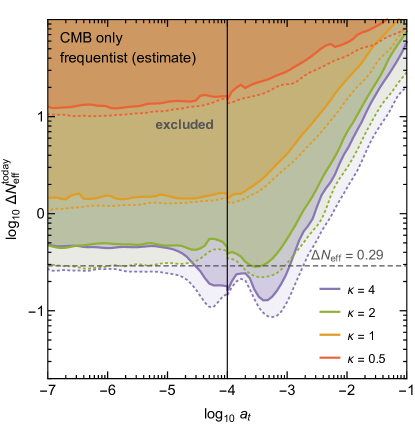
Figure 6: 95% C.L. (dotted lines) and 99% C.L. (solid lines) approximate frequentist constraints from CMB only; the coloured region above each line is excluded. Left panel. Constraints on the amount of converted DM. Right panel. Constraints on the amount of DR today, expressed in terms of $\Delta\tilde{N}_{\rm eff}$. For comparison we indicate the frequentist 95% C.L. bound on $\Delta\tilde{N}_{\rm eff}$ obtained from a scan with flat prior on $\Delta N_{\text{eff}}$ and $a_{t}=10^{-7}$ (derived from the 1D posterior shown in Fig. 4).

The discussion in the preceding paragraph has focussed on a qualitative understanding of the constraints on $\zeta$ shown in the left panel of Fig. 5. With the additional input from Fig. 1, it is straightforward to achieve a similar understanding concerning the qualitative shape of the constraints on $\Delta N_{\rm eff}$ as presented in the right panel of Fig. 5. In particular, the fact that these constraints are flat for small values of $a_{t}$ should not come as a surprise given that in this limits our model is expected to be indistinguishable from the case of a constant $\Delta N_{\rm eff}$. Quantitatively, however, the situation is less clear at first sight. In particular we infer from the right panel of Fig. 5 that for $\kappa=2,4$ and small $a_{t}$ values of $\Delta N_{\text{eff}}^{\text{today}}\gtrsim 0.7-0.8$ are excluded at 95% C.L. The reason for the difference between this value and the bound $\Delta N_{\text{eff}}^{\text{today}}\lesssim 0.4$ inferred from Fig. 4 is that here we consider the posterior pdf as a function of $\log_{10}\Delta N_{\text{eff}}^{\text{today}}$ rather than $\Delta N_{\text{eff}}^{\text{today}}$, which disfavours small values of $\log_{10}\Delta N_{\text{eff}}^{\text{today}}$ and hence introduces an overall bias towards larger values.

The prior dependence of the bounds shown in Fig. 5 makes it difficult to interpret them in a model-independent way. After all, $a_{t}$ and $\zeta$ are only effective parameters introduced to describe the evolution of the DM density, and the appropriate priors may depend sensitively on how this effect is realised in a more fundamental theory. A way to avoid this ambiguity is to consider frequentist rather than Bayesian exclusion limits. This is possible in a rather straight-forward manner thanks to the following two observations: First, since we consider flat priors on $\log_{10}a_{t}$ and $\zeta$ (or equivalently $\Delta N_{\text{eff}}^{\text{today}}$ for small $a_{t}$), the marginalised posterior as a function of these two parameters is directly proportional to the marginalised likelihood. Second, since all parameters apart from $a_{t}$ and $\zeta$ (or $\Delta N_{\text{eff}}^{\text{today}}$) are very well constrained by the CMB, the marginalised likelihood is expected to be similar to the profile likelihood (where for each value of $a_{t}$ and $\zeta$, or $\Delta N_{\text{eff}}^{\text{today}}$, all other parameters have been fixed to their best-fit value) Hamann (2012). We can therefore use the posterior probability to construct approximate profile likelihood ratios.

To construct frequentist upper bounds on the amount of DM that can be converted into DR, we determine the values of $a_{t}$ and $\zeta$ that give the best fit to the data, i.e. that maximise the posterior probability. For the data sets that we study in this section there is at most a very mild preference for non-zero $\zeta$, so that we typically find $\zeta_{\text{best}}\approx 0$. We then consider the test statistic

$$t=-2\,\Delta\log\mathcal{L}\approx-2\log\left[\frac{p(\zeta,a_{t})}{p(\zeta_{\text{best}},a_{t,\text{best}})}\right]\;,$$ (17)

where $p$ denotes the posterior probability. We expect that for random fluctuations in the data, $t$ will approximately follow a $\chi^{2}$ distribution with two degrees of freedom. We thus can exclude parameter points with $t>5.99$ ($t>9.21$) at 95% (99%) C.L.

We show the resulting estimate of frequentist exclusion limits on $\zeta$ in the left panel of Fig. 6. By construction, the frequentist exclusion limits follow lines of constant posterior probability and therefore have the same shape as the Bayesian exclusion limits shown in Fig. 5. In other words, the difference between the frequentist and the Bayesian exclusion limits is the confidence level associated to a specific posterior probability, i.e. frequentist exclusion limits correspond to Bayesian exclusion limits at a different confidence level. More specifically, we find the frequentist exclusion limits to be somewhat stronger.

The advantage of using frequentist exclusion limits is illustrated in the right panel of Fig. 6, which shows the bounds on $\Delta N_{\rm eff}$ calculated from the frequentist exclusion limits on $\zeta$ for $\kappa=2$ and $\kappa=4$. The only cosmological parameter required to perform this translation is $\Omega_{\chi}h^{2}$. Ideally, $\Delta N_{\rm eff}$ should be calculated using the respective best-fit value of $\Omega^{0}_{\chi}h^{2}$ for each value of $a_{t}$ and $\zeta$. However, given the precision of CMB constraints on this combination of DM density and expansion rate during recombination, it is sufficient to simply require $\Omega_{\chi}h^{2}=\Omega_{\chi}h^{2}|_{\Lambda\text{CDM}}$ at $z_{\text{rec}}\equiv 1100$.

In contrast to the bounds on $\Delta N_{\rm eff}$ shown in the right panel of Fig. 5, the bounds derived from the frequentist exclusion limits on $\zeta$ do not depend on the choice of priors for $\zeta$ and $a_{t}$. As a result, the bounds on $\Delta N_{\rm eff}$ obtained for small $a_{t}$ are much closer to the frequentist bounds derived from the 1D posterior shown in Fig. 4 (based on $a_{t}=10^{-7}$ and a flat prior on $\Delta N_{\text{eff}}$), which gives $\Delta N_{\text{eff}}<0.29$ for both $\kappa=2$ and $\kappa=4$ (indicated by the black dashed line). We will therefore from now on focus on frequentist exclusion limits. The corresponding Bayesian exclusion limits can be found in Appendix A.

IV Generic imprints on low-redshift observables

Let us now turn to the implications of converting DM to DR for low-redshift observables. We will focus here on the two most important late-time effects, namely a modified expansion rate and a change of the linear matter power spectrum $P(k)$. The former is something we briefly discussed already in Section II.1, cf. Fig. 2. Such a late-time enhancement of the Hubble rate may in principle help to reconcile a known discrepancy between low- and high-redshift observables Ade et al. (2014a); Raveri (2016); Bernal et al. (2016); Riess et al. (2016). In terms of possible physics realisations, such an option has so far mostly been discussed in terms of a constant DR (or sub-dominant hot DM) contribution Hou et al. (2013); Mehta et al. (2012); Wyman et al. (2014); Hamann and Hasenkamp (2013); Battye and Moss (2014); Costanzi et al. (2014) or decaying DM scenarios Enqvist et al. (2015); Berezhiani et al. (2015); Blackadder and Koushiappas (2016); Poulin et al. (2016); Chudaykin et al. (2016); Hamaguchi et al. (2017). By making the connection to our more general conversion scenario from DM to DR, we will revisit this question in a broader context.

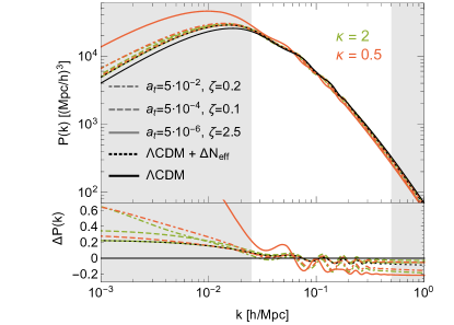
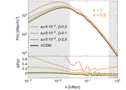
Figure 7: Linear matter power spectrum for the same set of benchmark models that we considered in Fig. 3. The range of wavenumbers that is not shaded gives the dominant contribution to $\sigma_{8}$. Left panel. $\Lambda$CDM parameters fixed to best-fit values from CMB only (as in left panel of Fig. 3). Right panel. $\Lambda$CDM parameters fixed to best-fit values from CMB+Lensing+HST+PC. Here the difference plot is still normalised to the $\Lambda$CDM power spectrum shown in the left panel.

Before doing so, however, let us briefly discuss the expected imprint on $P(k)$. To this end, we show in the left panel of Fig. 7 how the linear matter power spectrum changes, with respect to the $\Lambda$CDM case, for the same set of benchmark models (and $\Lambda$CDM parameters) that we considered in the left panel of Fig. 3. Note that the full non-linear power spectrum would be needed to make a meaningful comparison to data for large values of the wave-number $k$. For the present study we will therefore mostly limit ourselves to discussing the parameter combination $\sigma_{8}\Omega_{m}^{0.3}$, for which direct measurements exist Ade et al. (2014b) and to which mainly intermediate values of $k$ contribute, which are largely unaffected by non-linear dynamics. Specifically, $\sigma_{8}$ can be expressed as

$$\sigma_{8}^{2}=\frac{1}{2\pi^{2}}\int_{0}^{\infty}\text{d}k\,k^{2}P(k)\,W^{2}\left(kR_{8}\right)\,,$$ (18)

where $W(x)=3j_{1}(x)/x$ is the Fourier transform of the top-hat window function, $j_{1}$ is the first spherical Bessel function and $R_{8}\equiv 8\,h^{-1}\mathrm{Mpc}$. Requiring the integration range to contribute 99% to the value of $\sigma_{8}$, we find $0.025h\,\text{Mpc}^{-1}\lesssim k\lesssim 0.5h\,\text{Mpc}^{-1}$, which we indicate by the non-shaded region in Fig 7.

We first observe that on large scales, the spectrum is enhanced for our models. This is due to a larger value of $\Omega_{\Lambda}$, which enhances and shifts the spectrum towards larger scales Lesgourgues and Pastor (2006); Poulin et al. (2016). Secondly, for the range relevant for $\sigma_{8}$, we observe the spectrum to be suppressed. This is partially explained by a pure free streaming effect of the additional DR component (see the dotted line indicating the case of a constant $\Delta N_{\rm eff}$), and partially by the fact that perturbations evolve slightly different in our model than in $\Lambda$CDM, see Section II.2).

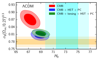
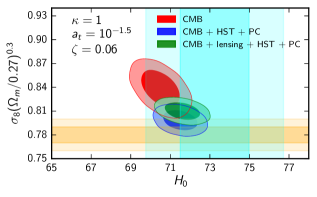
Figure 8: Best fit regions for $\Lambda$CDM (left panel) and our model with $\kappa=1$, $\zeta=0.06$ and $a_{t}=10^{-1.5}$ (right panel). The orange and cyan bands indicate the direct measurements of $\sigma_{8}(\Omega_{m}/0.27)^{0.3}=0.78\pm 0.01$ Ade et al. (2014b) and $H_{0}=73.24\pm 1.74$ Riess et al. (2016) respectively.

So far, we have included only CMB data in our discussion. In this section we extend our analysis to post-CMB cosmology by including the following data sets:

• CMB + Lensing: Same as CMB, with Planck lensing power spectrum reconstruction Ade et al. (2016b), using likelihoods as implemented in CosmoMC

• HST: Direct measurements of the Hubble rate $H_{0}=73.24\pm 1.74$ km/sec/Mpc by the Hubble space telescope Riess et al. (2016)

• PC: Measurement of the power spectrum normalisation, $\sigma_{8}(\Omega_{m}/0.27)^{0.30}=0.782\pm 0.010$, from the Planck Clusters Ade et al. (2014b).

In the right panel of Fig 7, we show how the matter power spectrum changes when using best-fit values of $\Lambda$CDM parameters from a simultaneous fit to all these datasets rather than CMB alone. On scales relevant for $\sigma_{8}$, this mostly has the effect of slightly increasing the power with respect to what is shown in the left panel of the same figure. This is due to the fact that for fitting the CMB spectrum of the model to the data, a smaller DM density of our model needs to be compensated by a larger $A_{s}$. Overall we thus typically expect a slightly larger value of $\sigma_{8}$ in our scenario, as compared to the $\Lambda$CDM case. While this seemingly further increases the discrepancy between CMB and low-redshift observables, we will see that the simultaneous decrease in $\Omega_{m}$ overcompensates this effect, allowing for a slight alleviation of the observed tension.

In Fig. 8, we provide a first illustration of the tension in low- and high-redshift observables mentioned above. The left panel, in particular, contrasts the $\Lambda$CDM best-fit region in the $H_{0}$ versus $\sigma_{8}(\Omega_{m}/0.27)^{0.30}$ plane obtained from CMB data only (red contours) with the direct measurements of these quantities by HST (cyan band) and PC (orange band). The blue contours show the preferred region in this plane when combining all these datasets. (the green contours result when also adding the Planck lensing power spectrum reconstruction Ade et al. (2016b)). The incompatibility between the different data sets is clearly visible and is in particular reflected in the fact that the red and blue ellipses do not overlap.

The right panel of Fig. 8 demonstrates how our conversion scenario may help to mitigate this discrepancy. For this purpose we show how the best-fit regions shift for specific values of our model parameters ($\kappa=1$, $a_{t}=10^{-1.5}$, $\zeta=0.06$). We note that such an efficient DM conversion would appear firmly excluded by the CMB limits shown in Fig. 5, but we will discuss below how adding large-scale structure data strongly relaxes those constraints (and, depending on the choice of priors, even prefers such large values of $\zeta$, see Appendix A. For this model point, we find that the red ellipse, corresponding to the parameter region preferred by the CMB alone, moves downward and to the right, such that it overlaps with the blue ellipse obtained from combining all data sets at 95% C.L.

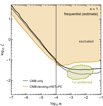
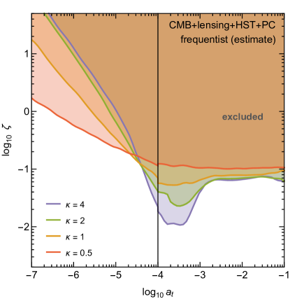
Figure 9: Left panel: Approximate frequentist constraints for our conversion scenario with $\kappa=1$, resulting from CMB+Lensing+HST+PC compared to the constraints obtained from CMB only (identical to the corresponding line in Fig. 5). The regions above the solid lines are excluded at 99% C.L. For CMB only we also show the 95% C.L. exclusion limit (dotted), while for CMB+Lensing+HST+PC we find a $\sim 2\sigma$ ‘signal’ preference and show the preferred parameter region at 68% C.L. (dashed). Right panel: Frequentist exclusion limits at 99% C.L. on the amount of converted DM from CMB+Lensing+HST+PC for different choices of $\kappa$.

We can qualitatively understand this effect by recalling that $\Omega_{\chi}h^{2}$ is tightly constrained at recombination. The decreasing DM component of our model at later times thus implies that we have to simultaneously increase the Hubble rate in order to remain compatible with CMB data. At the same time, the total matter density $\Omega_{m}=\Omega_{\chi}+\Omega_{b}$ also decreases, which shifts $\sigma_{8}(\Omega_{m}/0.27)^{0.30}$ downwards, even though $\sigma_{8}$ increases slightly with respect to the $\Lambda$CDM case (see Fig. 7). Including Lensing (green contours) slightly enhances the tension with the $\sigma_{8}$ measurement again, but does not change the picture qualitatively. We finally checked that adding Baryon Acoustic Oscillations measurements from the galaxy surveys in Refs. Beutler et al. (2011); Ross et al. (2015); Gil-Marín et al. (2016) would not affect the left panel of Fig. 8, but shift the blue contour in the right panel slightly to the left (to the point where the 1$\sigma$ contour does not quite overlap any more with the 1$\sigma$ band of the $H_{0}$ measurement).

Since our model of DM conversion clearly has the potential to reduce the tension between CMB and LSS data, we can expect that the inclusion of the latter will also significantly modify the constraints discussed in Sec. III. In the left panel of Fig. 9 we demonstrate this for the case of $\kappa=1$. The most prominent change compared to the bounds obtained from CMB data only is that constraints for large $a_{t}$ are substantially weaker. This is a direct consequence of the fact that in this region (and for $\zeta\sim 10^{-2}$) our model actually gives a better fit to data than $\Lambda$CDM (mostly by increasing the Hubble rate, as already indicated in Fig. 8). At the same time, the limits for small values of $a_{t}$ strengthen because CMB and LSS independently constrain a constant $\Delta N_{\rm eff}$. In the right panel of Fig. 9 we show the limits from CMB + Lensing + HST + PC for different choices of $\kappa$. In each case we observe a substantial weakening of the constraints for large $a_{t}$ compared to the limits obtained from CMB data only (see Figs. 5 and 6).

At this stage the obvious question arises whether our model of DM conversion only reduces the tension between CMB and LSS data, or whether one may even claim positive evidence for this model based on LSS data. From the frequentist perspective the preference is at the $\sim 2\sigma$ level and hence not very significant. We indicate in the right panel of Fig. 9 the parameter region preferred by the combination of CMB and LSS data at 68% C.L. From a Bayesian perspective, as discussed in more detail in Appendix A, the signal preference depends strongly on the adopted prior.

V Sommerfeld-enhanced dark matter annihilation

In this section we discuss DM with Sommerfeld enhancement as an interesting scenario in which a fraction of DM is converted into DR over a well-defined period of time. The basic idea is that DM particles interact with each other via a mediator particle with mass small compared to the DM mass, $m_{\text{med}}\ll m_{\chi}$. The exchange of light mediators then generates a potential that modifies the wave function of DM particles, leading to an enhancement of the DM self-annihilation cross section $(\sigma v)_{0}$ at small velocities Iengo (2009); Cassel (2010):

$$\sigma v=S(v)(\sigma v)_{0}\;.$$ (19)

As long as the Sommerfeld factor is small, $S(v)\approx 1$, the annihilation rate of a given DM particle decreases rapidly with decreasing redshift as the number density of DM particles decreases: $\Gamma_{\text{ann}}=\sigma v\,\rho_{\chi}/m_{\chi}\propto a^{-3}$. Since the Hubble rate decreases more slowly (proportional to $a^{-2}$ or $a^{-3/2}$ during radiation domination and matter domination, respectively), DM annihilations become less and less important in the late Universe.

This situation can be reversed in the presence of a large Sommerfeld enhancement. As we will discuss in more detail below, in certain regions of parameter space one finds $S(v)\propto v^{-2}$ for small velocities. As long as DM particles are in local thermal equilibrium, their velocity is $v\propto T_{\chi}^{1/2}\propto a^{-1/2}$. After the DM particles have kinetically decoupled from the heat bath, however, their momenta simply redshift as $v\propto a^{-1}$, such that $\Gamma_{\text{ann}}\propto a^{-1}$. In this case, the annihilation rate decreases more slowly than the Hubble rate and DM annihilations become increasingly important. This leads to a second period of DM annihilation after the classical chemical freeze-out Feng et al. (2010); van den Aarssen et al. (2012a). As a result, the comoving DM density may change appreciably at late times. For even smaller velocities, the Sommerfeld factor saturates and the DM annihilation rate reverts to its usual scaling proportional to $a^{-3}$, so that the comoving DM density again becomes constant.

V.1 Model set-up

To be more specific, we consider the case of a Dirac fermion DM particle $\chi$ coupled to a vector mediator $V^{\mu}$:

$$\mathcal{L}\supset g_{\chi}\,\bar{\chi}\gamma^{\mu}\chi V_{\mu}\;.$$ (20)

The dominant DM annihilation channel in this set-up is the s-wave process $\chi\bar{\chi}\to VV$, for which one finds, in the limit of vanishing relative velocity and mediator mass, $(\sigma v)_{0}=\pi\alpha^{2}/m_{\chi}^{2}$ with $\alpha=g_{\chi}^{2}/(4\pi)$. Although the mediators produced in DM annihilations could themselves act as DR, we assume that they subsequently decay into even lighter particles, such as sterile neutrinos. The advantage of such a set-up is that the resulting interactions between DM and DR can significantly delay the kinetic decoupling of DM van den Aarssen et al. (2012b) (while at the same time avoiding strong CMB constraints on visible decays Bringmann et al. (2017)). Rather than specifying the coupling between the mediator and DR, however, we introduce here the kinetic decoupling temperature $T_{\text{kd}}$ as an additional free parameter to keep the discussion more model-independent. In Sec. V.5 we will briefly get back to the range of decoupling temperatures that would be expected in the simplest extension to the model specified in Eq. (20), and otherwise refer to Ref. Bringmann et al. (2016) for a detailed discussion of how late kinetic decoupling can be achieved in general.

The exchange of vector mediators generates the Yukawa potential

$$V(r)=\frac{\alpha\,e^{-r\,m_{\text{med}}}}{r}\;.$$ (21)

The Sommerfeld factor can be calculated analytically by approximating the Yukawa potential with a Hulthén potential, giving Iengo (2009); Cassel (2010); Tulin et al. (2013)

$$S=\frac{2\pi\,\alpha\sinh\left(\frac{6m_{\chi}v}{\pi m_{\text{med}}}\right)}{v\left[-\cos\left(2\pi\sqrt{\frac{6m_{\chi}\alpha}{\pi^{2}m_{\text{med}}}-\frac{9m_{\chi}^{2}v^{2}}{\pi^{4}m_{\text{med}}^{2}}}\right)+\cosh\left(\frac{6m_{\chi}v}{\pi m_{\text{med}}}\right)\right]}\;.$$ (22)

We display this Sommerfeld enhancement factor in Fig. 10 as a function of $m_{\text{med}}$ for fixed values of $m_{\chi}$, $\alpha$ and $v$.

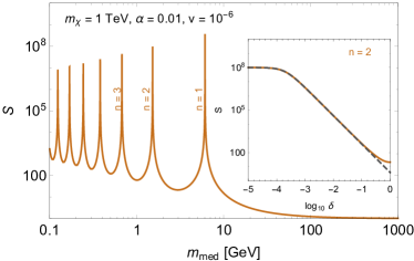
Figure 10: Sommerfeld enhancement factor $S$ as a function of $m_{\text{med}}$ for fixed values of $m_{\chi}$, $\alpha$ and $v$. If the mediator mass satisfies Eq. (23) for some integer $n$ the enhancement can be very large. In the inset we zoom into one specific resonance ($n=2$) by replacing $m_{\text{med}}$ with $\delta$ as defined in Eq. (24). For comparison we also show the approximation of the Sommerfeld enhancement factor given in Eq. (25), which is valid for $\delta\ll 1/(n\pi)$ and $v\ll\alpha/(n^{2}\pi)$.

In the limit of vanishing velocities, one finds that the denominator becomes very small if

$$m_{\text{med}}\approx\frac{6m_{\chi}\alpha}{\pi^{2}n^{2}}$$ (23)

for some integer $n$. To quantify how close a specific parameter point is to such a resonance, we define

$$\delta\equiv\left|\frac{m_{\text{med}}-m_{\text{med}}^{(n)}}{m_{\text{med}}^{(n)}}\right|\equiv\left|1-\frac{\pi^{2}n^{2}\,m_{\text{med}}}{6m_{\chi}\alpha}\right|\;,$$ (24)

where $m_{\text{med}}^{(n)}$ is the value of $m_{\text{med}}$ at the $n$th resonance and $n$ is chosen to minimise $\delta$. The inset in Fig. 10 shows the Sommerfeld factor as a function of $\delta$ for $n=2$.

If $\delta$ is sufficiently small, $\delta\ll 1/(n\pi)$, one finds that the Sommerfeld factor for small velocities, $v\ll\alpha/(n^{2}\pi)$, can be written as

$$S(v)=\frac{4\alpha^{2}}{n^{2}v^{2}+\alpha^{2}\delta^{2}}\;.$$ (25)

The quality of this approximation can be inferred from the black dashed line in the inset of Fig. 10. We conclude that the Sommerfeld factor begins to grow as $1/v^{2}$ until $v\lesssim v_{\text{sat}}\equiv\alpha\delta/n$, at which point the Sommerfeld factor saturates at $S\approx 4/\delta^{2}$.

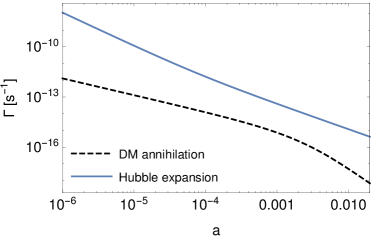
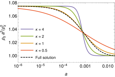
Figure 11: Left panel. Hubble expansion rate (solid line) compared to the annihilation rate of a given DM particle (dashed line) with $m_{\chi}=250\,\text{GeV}$, $\alpha=10^{-2}$, $n=10$, $\delta=10^{-5}$ (corresponding to a mediator mass $m_{\text{med}}\approx 13$ MeV) and kinetic decoupling temperature $T_{\text{kd}}=1\,\text{keV}$. Right panel. Resulting DM density evolution for the same parameter point as in the left panel (dashed line), compared to the phenomenological transition scenarios introduced in Section II for $a_{t}=7.2\cdot 10^{-4}$ and $\zeta=0.075$ (solid lines; see also Fig. 1).

An additional subtlety is that the Sommerfeld factor obtained from the naive solution of the Hulthén potential can become so large that the annihilation cross section violates unitarity at very small velocities. To avoid this unitarity violation for very small $\delta$, we follow the prescription from Ref. Blum et al. (2016) and consider the modified Sommerfeld factor

$$S(v)=\frac{4\alpha^{2}}{n^{2}\left(v+v_{c}\right)^{2}+\alpha^{2}\delta^{2}}$$ (26)

with $v_{c}=\alpha^{4}/(4n^{2})$.

We emphasise that while Eq. (26) provides a very good approximation to the Sommerfeld factor close to resonance at small velocities, it does not yield the correct description for large velocities or far away from a resonance. However, as argued above, DM annihilations will not be important in these regimes anyways, so that a more detailed modelling of the Sommerfeld factor is unnecessary for our purposes. We also note that the way in which we implement the restoration of unitarity for small $\delta$ is only approximate. While it ensures that the Sommerfeld factor does not exhibit unphysical behaviour for $v\to 0$, we expect a more detailed calculation to yield slightly different results for finite velocities.

V.2 Evolution of dark matter density

For the purpose of calculating DM annihilation rates, we are interested in the thermally averaged annihilation cross section

$$\langle\sigma v_{\text{rel}}\rangle=\langle S(\sigma v_{\text{rel}})_{0}\rangle=\langle S\rangle(\sigma v_{\text{rel}})_{0}\;,$$ (27)

where we have made use of the fact that $(\sigma v)_{0}$ is independent of velocity. To calculate the thermal average, we assume that the DM velocity distribution is given by a Maxwell-Boltzmann distribution with an effective temperature $T_{\text{eff}}$:

$$f(v_{\text{rel}})=\sqrt{\frac{x_{\text{eff}}^{3}}{4\pi}}v_{\text{rel}}^{2}\exp\left(-\frac{v_{\text{rel}}^{2}\,x_{\text{eff}}}{4}\right)\;,$$ (28)

where we have introduced the dimensionless temperature $x_{\text{eff}}=m_{\chi}/T_{\text{eff}}$. We note that the above ansatz is automatically satisfied for parameter combinations close to a resonance because the same light mediator that causes the Sommerfeld enhancement also guarantees very efficient DM self-interactions van den Aarssen et al. (2012a).

In order to proceed, we need to express $x_{\text{eff}}$ as a function of the scale factor $a$. For this purpose, we assume that DM particles are no longer in kinetic equilibrium with the thermal bath. Denoting the temperature and scale factor of kinetic decoupling by $T_{\text{kd}}$ and $a_{\text{kd}}$, respectively, we find

$$T_{\text{eff}}=T_{\text{kd}}\frac{a_{\text{kd}}^{2}}{a^{2}}=\frac{T_{0}^{2}}{T_{\text{kd}}}a^{-2}\;,$$ (29)

where $T_{0}$ is the present-day photon temperature. We conclude that the thermally averaged Sommerfeld factor is proportional to $a^{2}$ for $a\lesssim a_{\text{sat}}\equiv T_{0}/(v_{\text{sat}}\sqrt{T_{\text{kd}}m_{\chi}})$ and becomes constant for larger scale factors.

We show the corresponding DM annihilation rate $\Gamma_{\text{ann}}$ in comparison to the Hubble rate in the left panel of Fig. 11 for $m_{\chi}=250\,\text{GeV}$, $\alpha=10^{-2}$, $n=10$, $\delta=10^{-5}$ and $T_{\text{kd}}=1\,\text{keV}$, corresponding to a mediator mass of $m_{\text{med}}\approx 13$ MeV (the value of $\alpha$ was chosen such as to roughly result in the correct relic density from standard thermal freeze-out). For this choice of parameters the Sommerfeld factor saturates around $a\sim 10^{-3}$, staying significantly below the Hubble rate.

To calculate the change of DM density resulting from this annihilation rate, we need to solve the Boltzmann equation

$$\frac{\mathrm{d}\rho_{\chi}}{\mathrm{d}z}(1+z)H(z)-3\rho_{\chi}H(z)-\frac{1}{2}\langle\sigma v_{\text{rel}}\rangle\frac{\rho_{\chi}^{2}}{m_{\chi}}=0$$ (30)

with the boundary condition

$$\rho_{\chi}(z_{\text{CMB}})=\Omega_{\chi}\rho_{c}(1+z_{\text{CMB}})^{3}\;,$$ (31)

where $z_{\text{CMB}}=1100$ is the redshift at recombination and $\Omega_{\chi}=0.1198/h^{2}$ and $\rho_{c}=1.054\cdot 10^{-5}h^{2}\mathrm{GeV/cm^{3}}$ are the present-day DM abundance and critical density inferred from CMB observations under the assumption of $\Lambda$CDM. The factor of $1/2$ in front of the last term in Eq. (30) accounts for the fact that DM consists of Dirac particles; in other words, $\rho_{\chi}$ refers here to the total density of both $\chi$ and $\bar{\chi}$ and thus has the same meaning as in the previous sections. The solution of this equation is shown in the right panel of Fig. 11 for the same choice of parameters as on the left (black dashed line). We also show for comparison the DM density as a function of redshift for the phenomenological parametrisation introduced in Section II. We find that for $\kappa=1$ (orange line) the model is very similar to the numerical solution of the Boltzmann equation, while for the other values of $\kappa$ the transition looks quite different.

V.3 CMB and LSS constraints

We just concluded that late-time DM annihilations with resonant Sommerfeld enhancement provide a good example for the model discussed in the previous sections with $\kappa=1$. We can therefore use the constraints obtained for that phenomenological model to place bounds on models with resonant Sommerfeld enhancement. In order to determine whether a specific parameter point is allowed or excluded by cosmological data, we thus need to determine the values of $a_{t}$ and $\zeta$ that provide the best fit to the numerical solution of the Boltzmann equation and then compare these values to the frequentist bounds shown in Fig. 9 (concretely, we determine $a_{t}$ as the scale factor where half of the conversion has happened). Using frequentist bounds has the crucial advantage that we do not need to specify priors for the particle physics parameters of the model we consider. Moreover, even if priors for the particle physics parameters could be motivated, these would likely translate to non-trivial priors on $a_{t}$ and $\zeta$, meaning that the Bayesian limits derived in the previous section could not be directly applied.

From the discussion in the previous subsection, this translation to $a_{t}$ and $\zeta$ can be done for arbitrary combinations of $m_{\chi}$, $\alpha$, $n$, $\delta$ and $T_{\text{kd}}$ that satisfy the following conditions:

• The parameter point lies in the resonant regime: $\delta\ll 1/(n\pi)$.

• Kinetic decoupling happens before the Sommerfeld factor saturates: $T_{\text{kd}}\gg m_{\chi}\,v_{\text{sat}}^{2}$.

• The DM annihilation rate stays significantly below the Hubble rate even for $a\approx a_{\text{sat}}$, so that the total relative change of the DM density remains small: $\zeta\lesssim 1$.

While the last requirement is not strictly necessary, it becomes computationally very challenging to accurately calculate the evolution of the DM density for $\zeta>1$ due to the need to account for changes in the temperature of the dark sector. As we will see below, parameter regions with $\zeta>1$ are either robustly excluded or phenomenologically uninteresting, so that we do not consider these regions in more detail.

In the following, we will impose one additional requirement, namely that $\alpha$ is chosen in such a way that the DM abundance predicted from thermal freeze-out coincides with the solution of Eq. (30) for very early times, i.e. $a\ll a_{\text{sat}}$. This requires solving the Boltzmann equation iteratively until a self-consistent solution is found. We note that such an iterative procedure is particularly important for the parameter region where unitarity restoration plays a role, because in this case the saturated Sommerfeld factor is proportional to $\alpha^{-6}$.

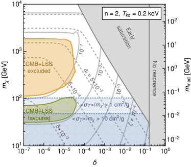
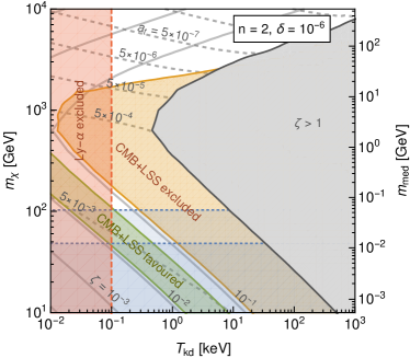
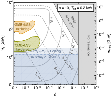
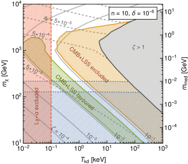
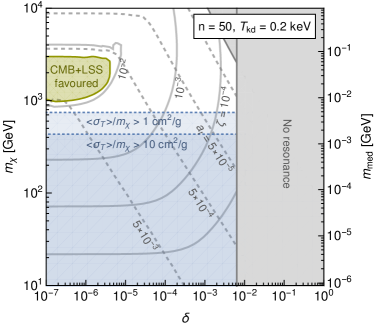
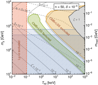
Figure 12: Constraints on DM with Sommerfeld enhancement as a function of $m_{\chi}$ and $\delta$ (left) and as a function of $m_{\chi}$ and $T_{\text{kd}}$ (right). The different rows correspond to different resonances, i.e. different choices of $n$. The second $y$-axis in each panel indicates the mediator mass $m_{\text{med}}$ corresponding to $m_{\chi}$ for the specific resonance, cf. Eq. (23).

A final complication arises from the onset of non-linear structure formation around $z_{\text{nl}}\approx 50$. At this point the DM particles decouple from the Hubble flow, and their relative velocities start to increase. As a result the Sommerfeld enhancement factor drops and the comoving DM density very quickly becomes constant for $z\lesssim z_{\text{nl}}$, even if the Sommerfeld factor has not yet saturated. In this case, the functional form introduced in Eq. (1) no longer provides a good description of the redshift dependence of the DM density for $a\gtrsim a_{t}$ (when choosing $a_{t}$ as the scale factor where half of the conversion has happened). However, as seen in Fig. 9, if the conversion of DM to DR happens sufficiently after recombination, constraints are largely insensitive to the precise redshift dependence and only limit the total amount of DM converted. We can therefore continue to use the phenomenological parametrisation from above even in this regime. The cut-off of DM annihilations by non-linear structure formation can be shown to impose $a_{t}\gtrsim 7\cdot 10^{-3}$ in our model.

Our results are summarised in Fig. 12 for $n=2$ (top row), $n=10$ (middle) and $n=50$ (bottom row). In the left column we fix $T_{\text{kd}}=0.2\,\mathrm{keV}$ and vary $\delta$, in the right column we fix $\delta=10^{-6}$ and vary $T_{\text{kd}}$. The solid (dashed) lines in each panel indicate combinations of $m_{\chi}$ and $\delta$ corresponding to constant $\zeta$ (constant $a_{t}$). The yellow shaded region in each panel indicates the region of parameter space excluded by the constraints derived in this work, while the green shaded regions indicate the region favoured by combining CMB and LSS data (as also shown in Fig. 9). The parameter regions that violate one or more of our basic conditions i) – iii) are shaded in grey.

As expected, and as directly visible in the left panel of the figure, CMB and LSS data can only probe our model in the case of very small values of $\delta$, i.e. for parameter regions rather close to a resonance. Interestingly, for each value of $n$, and a given kinetic decoupling temperature, only a finite range of DM masses is excluded and preferred, respectively; these mass ranges move to larger values with increasing $n$. We note that the upper value of the excluded DM mass range is driven by the saturation of the Sommerfeld enhancement for very small velocities and $\delta$, so this is where the improvement of Eq. (25) to Eq. (26) is most relevant. Increasing $T_{\text{kd}}$, as in the right column, has the effect of lowering the DM mass preferred by the data; the range of excluded DM mass is increased. We will soon see, however, that too small DM masses inevitably lead to an unacceptably large DM self-scattering rate, so in practice it is not very interesting to consider kinetic decoupling temperatures much larger than 1 keV in this model.

V.4 Discussion

Let us briefly return to the treatment of perturbations in our conversion scenario. In Sec. II.2 we argued that this is necessarily model-dependent, i.e. not uniquely determined by the choice of parameters $(\kappa,\zeta,a_{t})$ that describe the evolution of the background densities. Concretely we have so far always adopted the minimal option stated in Eq. (13), i.e.

$$\delta\mathcal{Q}/Q=\delta_{\chi}\,.$$ (32)

For the case studied in this section the situation is different, because the conversion rate $\mathcal{Q}$ is associated to a concrete microphysics process, so that the Boltzmann equation directly determines the form of $\delta\mathcal{Q}$. The case of off-resonance Sommerfeld enhancement was discussed e.g. in Ref. Armendariz-Picon and Neelakanta (2012), but the fully general case is rather involved. We will therefore estimate the impact of perturbations using a simplified treatment based on heuristic arguments.

For annihilation processes with two DM particles in the initial state, we have $\mathcal{Q}\propto\langle\sigma v\rangle\rho^{2}_{\chi}$, and thus

$$\delta\mathcal{Q} =\frac{\partial\mathcal{Q}}{\partial\langle\sigma v\rangle}\delta\langle\sigma v\rangle+\frac{\partial\mathcal{Q}}{\partial\rho_{\chi}}\delta\rho_{\chi}=\frac{\delta\langle\sigma v\rangle}{\langle\sigma v\rangle}\mathcal{Q}+2\mathcal{Q}\,\delta_{\chi}\,.$$ (33)

For $\sigma v\propto v^{-1}$, the perturbation $\delta\langle\sigma v\rangle$ at large scales is given by $\delta\langle\sigma v\rangle=\langle\sigma v\rangle\,\frac{h}{6}$ Armendariz-Picon and Neelakanta (2012). Following the heuristic arguments given in that reference, this can be generalised to $\delta\langle\sigma v\rangle=\beta\langle\sigma v\rangle\,\frac{h}{6}$ for a cross section scaling with velocity as $\sigma v\propto v^{-\beta}$. Since we are mostly interested in parameter combinations very close to a resonance, where $\sigma v\propto v^{-2}$ this motivates us to change the prescription for perturbations to

$$\delta\mathcal{Q}/Q=\delta_{\chi}\to\frac{1}{3}h+2\delta_{\chi}\,.$$ (34)

This enters in both the evolution equation for DM perturbations, Eq. (11), and in those for the DR perturbations, Eqs. (14,15).

In Fig. 13 we demonstrate that this change hardly affects the frequentist limits and preferred region for the $\kappa=1$ model. This confirms our expectation from Sec. II.2 that the impact of perturbations should typically be small, implying that one generally can directly adopt the results shown in the previous sections (in particular Figs. 5 and 9). We stress, however, that this remains a model-dependent statement, which in principle has to be checked on a case-by-case basis (as we have done here).

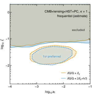
Figure 13: Solid lines show the 99% C.L. approximate frequentist limits and dotted lines the 68% C.L. preferred parameter region for our conversion scenario with $\kappa=1$, resulting from CMB+Lensing+HST+PC. The orange and green areas result from our standard treatment of perturbations and are identical to those shown in the right panel of Fig. 9. The blue lines and area result when changing this prescription as stated in Eq. (34).

Let us finally briefly discuss the case that the dark sector (i.e. DM and DR) is colder than the visible sector during thermal freeze-out, $\xi\equiv T_{\text{dark}}/T_{\text{vis}}<1$. Such a situation occurs naturally if the two sectors only interact with each other at very high temperatures but then evolve independently. In fact, it is probably necessary to have $\xi<1$ in order to avoid an unacceptably large contribution to $N_{\text{eff}}$ from DR (see, e.g., Ref. Bringmann et al. (2016)). A non-trivial temperature ratio has three effects: it reduces the value of $\alpha$ required to reproduce the observed DM relic abundance, it reduces the velocity of DM particles for a given temperature of the visible sector, and it leads to earlier kinetic decoupling (see below). In combination, these three effects result in a larger Sommerfeld factor at early times but smaller saturation value, implying in particular that the saturation happens earlier Binder et al. (2018). A quantitative discussion of the resulting changes requires more specific assumptions and is thus beyond the scope of this work.

V.5 Impact on small scales

The model that we have studied in this section has a number of further interesting properties, which allow us to extend the discussion of Fig. 12 to additional cosmological and astrophysical observables. First of all, an interaction as given in Eq. (20) inevitably mediates a strong DM self-interaction for the light mediators that we consider here. In the resonant regime, the self-interaction cross section can again be calculated by approximating the Yukawa potential by a Hulthén potential. Close to a resonance (i.e. for $\delta\ll 1$), the phase shift from the scattering process is very close to $\pi/2$ and one therefore obtains the simple expression

$$\sigma_{\mathrm{T}}=\frac{16\pi}{m_{\chi}^{2}\,v_{\text{rel}}^{2}}\;.$$ (35)

For $m_{\chi}v/m_{\text{med}}\gtrsim 1$, corresponding to $n^{2}v/\alpha\gtrsim 1$, the Hulthén approximation becomes inaccurate and a better solution is obtained by fitting to numerical solutions of the Schroedinger equation. We adopt the parametrisation for this classical regime from Ref. Cyr-Racine et al. (2016), noting that in this case the momentum transfer cross section scales approximately as $\sigma_{\mathrm{T}}\propto(n/m_{\chi})^{3\text{--}4}$.

In all panels of Fig. 12 we indicate the parameter regions $\langle\sigma_{\mathrm{T}}\rangle/m_{\chi}>10\,\mathrm{cm^{2}/g}$, where $\langle\sigma_{\mathrm{T}}\rangle$ denotes the velocity-averaged momentum transfer cross section for a typical relative velocity of $30\,\mathrm{km/s}$. This parameter region is robustly excluded by bounds from dwarf spheroidal galaxies and low-surface-brightness galaxies Tulin and Yu (2018); Valli and Yu (2017); Bondarenko et al. (2018) and simply corresponds to an upper bound on the DM mass that only depends on $n$. It is worth noting that DM self-interactions with somewhat smaller cross sections, and correspondingly larger DM masses, have been independently invoked Loeb and Weiner (2011); Vogelsberger et al. (2012); Peter et al. (2013); Zavala et al. (2013); van den Aarssen et al. (2012b); Elbert et al. (2015); Kamada et al. (2017); Robertson et al. (2017) to mitigate a number of long-standing small-scale problems of structure formation, namely the cusp-versus-core de Blok and McGaugh (1997); Oh et al. (2011); Walker and Penarrubia (2011) and the too-big-to-fail problem Boylan-Kolchin et al. (2011); Papastergis et al. (2015) (as well as, more recently, the diversity problem Oman et al. (2015, 2016); Robertson et al. (2017)). As can be seen in the figure, such self-interaction rates can relatively easily be accommodated in our model for parameter values that also are favoured by the CMB+LSS data – in particular for large values of $n$.

As already mentioned, these strong constraints from DM self-interactions imply rather small kinetic decoupling temperatures when compared to standard WIMP candidates. Such a late kinetic decoupling introduces a small-scale cut-off in the matter power spectrum similar to warm DM Vogelsberger et al. (2016). Thus, $T_{\mathrm{kd}}$ cannot be too small without being in conflict with Lyman-$\alpha$ forest observations. In the right column of Fig. 12 we therefore also show a rough estimate of this bound, $T_{\text{kd}}\gtrsim 0.1\,\mathrm{keV}$ Bringmann et al. (2016); Huo et al. (2018). Kinetic decoupling temperatures close to this bound may lead to the suppression of small-scale structure and thereby alleviate yet another long-standing small-scale issue of $\Lambda$CDM cosmology, namely the missing satellites problem Moore et al. (1999); Klypin et al. (1999); Fattahi et al. (2016) (see however Jethwa et al. (2018); Huo et al. (2018); Kim et al. (2017) for recent discussions of this issue). Fig. 12 thus suggests that this is possible in the same parameter region that is favoured by large-scale data and DM self-interactions at dwarf galaxy scales – (almost) independent of which resonance, $n$, is considered.

At this point, however, we should recall that $T_{\mathrm{kd}}$ is not really a free parameter but is in principle uniquely determined by the DM particle model. The simplest possibility would be to couple the mediator $V_{\mu}$ not only to DM but also to DR, with a coupling $g_{\phi}=\eta g_{\chi}$. This results in Bringmann et al. (2016)

$$T_{\mathrm{kd}}^{\mathrm{simp}} \sim 0.3\,\mathrm{keV}\times\eta^{-1/2}\xi^{-3/2}\left(\frac{m_{\chi}}{\mathrm{TeV}}\right)^{-1/4}\left(\frac{m_{\mathrm{med}}}{\mathrm{MeV}}\right)$$

$$\sim 0.7\,\mathrm{keV}\left(\frac{n}{100}\right)^{2}\times\eta^{-1/2}\xi^{-3/2}\left(\frac{m_{\chi}}{\mathrm{TeV}}\right)^{7/4}\;,$$ (36)

where $\xi$ denotes the temperature ratio of dark to visible sector. This clearly shows that it is in practice difficult to achieve late kinetic decoupling for mediator masses above the MeV scale. Combining this insight with the self-interaction bounds shown in the right column of Fig. 12, we conclude that this affects resonant annihilation for small $n$.

On the other hand, we make the interesting observation that for TeV-scale DM and ’high’ resonances, with $n\gtrsim 50$, it is in fact rather straightforward to simultaneously alleviate the missing satellites and other small-scale problems, and at the same time reduce the $H_{0}$ and $\sigma_{8}$ tensions. Given that we adopted a rather minimal model set-up, this is an intriguing result. The fact that (various combinations of) these tensions between observations and the cosmological concordance model can be simultaneously addressed for similar models has been pointed out before Loeb and Weiner (2011); Vogelsberger et al. (2012); van den Aarssen et al. (2012b); Dasgupta and Kopp (2014); Bringmann et al. (2014); Huo et al. (2018); Binder et al. (2018); here we confirmed those claims, adding the first full combined analysis of CMB and LSS data in this context.

VI Conclusions

The cosmological concordance model rests on the somewhat bold assumption that the comoving DM density remains exactly constant while the Universe expands in volume by more than 20 orders of magnitude. In this article we have quantified how strongly deviations from this scenario are constrained observationally. In order to do so in as model-independent and conservative a way as possible, we have assumed a range of phenomenological transition scenarios (see Fig. 1) where DM is converted into a non-interacting form of radiation.

We find that all scenarios where the DM density is reduced by more than a few percent after matter-radiation equality are in strong tension with CMB observations (see Fig. 5). For earlier transitions, on the other hand, a much larger fraction of DM can be converted; this is expected given that the relative contribution of DM to the total energy budget is correspondingly smaller. Adding low-redshift observables to the analysis relaxes the late-time constraints, cf. Fig. 9, allowing up to around 10 percent of DM to be converted during matter domination.

The reason for the weakening of the CMB constraints is that a late conversion from DM to DR reduces the well-known tension between these essentially incompatible datasets. We discussed in detail in what sense this implies positive evidence for such a transition scenario, concluding that, from a frequentist perspective, the preference is rather mild. We stressed, however, that a Bayesian analysis would come to a very different conclusion for a prior choice that puts special emphasis on late-time conversions (see Appendix A).

We argued that our parametrisation of possible transition scenarios from DM to DR is very general and encompasses those previously discussed in the literature, in particular the case of decaying DM (see again Fig. 1). Another interesting application would be primordial black hole DM, where merger events inevitably transform part of the black hole mass to DR in the form of gravitational waves. In the last part of this work, Section V, we have discussed in detail yet another scenario that can be mapped to our general parametrisation, namely DM coupled to DR via light mediator particles. For specific values of the mediator mass, cf. Fig. 12, this implies a strongly enhanced DM annihilation rate at late times that can mitigate the above-mentioned tension between CMB and large-scale structure data. Remarkably, as we have also discussed, such a simple scenario could simultaneously alleviate the most pressing $\Lambda$CDM problems at small scales.

Turning this around, there is a surprising variety of astrophysical and cosmological observations that allow to test such a simple particle model even though it is almost fully confined to a dark sector, with negligible couplings to the Standard Model. The constraints derived in this work are thus not only of general interest, in the sense that they quantify how well one of the basic assumptions of the cosmological concordance model is tested observationally, but can very concretely help to test and discriminate a variety of (particle) DM models.

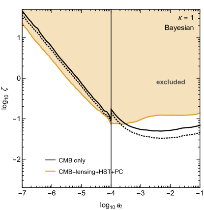
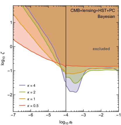
Figure 14: Left panel: 95% C.L. (dotted lines) and 99% C.L. (solid lines) Bayesian limits for our conversion scenario with $\kappa=1$, resulting from CMB+Lensing+HST+PC. For comparison we also show the constraints obtained from CMB only (identical to the corresponding line in Fig. 5). Right panel: Bayesian limits on the amount of converted DM from CMB+Lensing+HST+PC for different choices of $\kappa$; the coloured region above each line is excluded.

Acknowledgements.—

We thank Tobias Binder, Thejs Brinckmann, Jens Chluba, Michael Gustafsson, Anders Kvellestad and Julien Lesgourgues for very useful discussions. This work is supported by the German Science Foundation (DFG) under the Collaborative Research Center (SFB) 676 “Particles, Strings and the Early Universe” and the Emmy Noether Grant No. KA 4662/1-1 as well as the ERC Starting Grant ‘NewAve’ (638528). PW is partially supported by the University of Oslo through the Strategic Dark Matter Initiative (SDI).

Appendix A Bayesian exclusion limits

In this Appendix we complement the discussion in Section IV with a Bayesian perspective on our general conversion scenario. We start by showing in Fig. 14 the Bayesian exclusion limits corresponding to the approximate frequentist exclusion limits shown in Fig. 9. These limits are obtained using flat priors on $\log a_{t}$ and $\zeta$ (for $a_{t}>10^{-4}$) or $\Delta N_{\rm eff}^{\rm today}$ (for $a_{t}<10^{-4}$). In contrast to the $\sim 2\sigma$ preference for our model found in the frequentist approach, a Bayesian model comparison actually favours $\Lambda$CDM, as the parameter region in which the extended model is preferred over $\Lambda$CDM is much smaller than the parameter region in which the model is strongly disfavoured. This conclusion nevertheless depends strongly on the priors assumed for our effective description and could be modified in a set-up where favourable values of $a_{t}$ and $\zeta$ occur naturally.

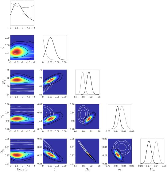
Figure 15: Marginalised 2D and 1D posteriors resulting from CMB+Lensing+HST+PC for our conversion scenario with $\kappa=1$, with closed contours indicating 68%, 95% and 99% C.L., respectively. The white contours (in the 2D plots) and grey lines (in the 1D plots) are for CMB only.

In Fig. 15 we provide a supplementary perspective on our discussion so far, which also illustrates the point just made. We show the marginalised 1D and 2D posteriors for our model parameters as well as the $\Lambda$CDM parameters most relevant in our context, namely $H_{0}$, $\sigma_{8}$ and $\Omega_{m}$. We do so both for CMB only (grey lines and white contours) and CMB + Lensing + HST + PC (black lines and coloured contours), respectively. Here, we have fixed $\kappa=1$ and chosen a flat prior for $\zeta$; for $\log_{10}a_{t}$ we have chosen a flat prior between $-3$ and $-1$, thus zooming in on the most relevant parameter region. For such a prior choice we see a clear signal preference in the $\zeta$ vs. $\log_{10}a_{t}$ plane, once we add LSS data, which can directly be compared to Fig. 9.

It is also illuminating to see the correlation of our model parameters with the cosmological observables considered here. For example, it becomes obvious that the degeneracy between matter density and Hubble rate is not broken when adding LSS data. This motivates previous statements that $\Omega_{\chi}h^{2}$ is very well constrained both in $\Lambda$CDM and in our scenario, and confirms our qualitative discussion of Fig. 8. There we argued that a larger Hubble rate at late times not only helps to reconcile direct measurements of $H_{0}$ but automatically, due to this degeneracy, the direct measurement of the parameter combination $\sigma_{8}\Omega_{m}^{0.3}$ as well. As a result of combining essentially incompatible data sets, the parameters that have been marginalised out are thus pushed towards values that reduce the tension between CMB and LSS data. In our case, as can explicitly be seen in the corresponding 2D posteriors in Fig. 15, this independently results in large values for $a_{t}$ and $\zeta$. Let us stress again that these conclusions are prior dependent; allowing $\log_{10}a_{t}$ to extend to much smaller values, for example, fully erases the preference for a signal around $a_{t}\sim 10^{-2.5}$ and $\zeta\sim 0.03$.

References

- Ade et al. (2016a) P. A. R. Ade et al. (Planck), Astron. Astrophys. 594, A13 (2016a), arXiv:1502.01589 [astro-ph.CO] .
- Lee and Weinberg (1977) B. W. Lee and S. Weinberg, Phys. Rev. Lett. 39, 165 (1977).
- Gondolo and Gelmini (1991) P. Gondolo and G. Gelmini, Nucl. Phys. B360, 145 (1991).
- Cirelli et al. (2012) M. Cirelli, E. Moulin, P. Panci, P. D. Serpico, and A. Viana, Phys. Rev. D86, 083506 (2012), arXiv:1205.5283 [astro-ph.CO] .
- Ibarra et al. (2013) A. Ibarra, D. Tran, and C. Weniger, Int. J. Mod. Phys. A28, 1330040 (2013), arXiv:1307.6434 [hep-ph] .
- Poulin et al. (2017) V. Poulin, J. Lesgourgues, and P. D. Serpico, JCAP 1703, 043 (2017), arXiv:1610.10051 [astro-ph.CO] .
- Zentner and Walker (2002) A. R. Zentner and T. P. Walker, Phys. Rev. D65, 063506 (2002), arXiv:astro-ph/0110533 [astro-ph] .
- Ichiki et al. (2004) K. Ichiki, M. Oguri, and K. Takahashi, Phys. Rev. Lett. 93, 071302 (2004), arXiv:astro-ph/0403164 [astro-ph] .
- Lattanzi and Valle (2007) M. Lattanzi and J. W. F. Valle, Phys. Rev. Lett. 99, 121301 (2007), arXiv:0705.2406 [astro-ph] .
- Peter (2010) A. H. G. Peter, Phys. Rev. D81, 083511 (2010), arXiv:1001.3870 [astro-ph.CO] .
- Wang and Zentner (2010) M.-Y. Wang and A. R. Zentner, Phys. Rev. D82, 123507 (2010), arXiv:1011.2774 [astro-ph.CO] .
- Bjaelde et al. (2012) O. E. Bjaelde, S. Das, and A. Moss, JCAP 1210, 017 (2012), arXiv:1205.0553 [astro-ph.CO] .
- Allahverdi et al. (2015) R. Allahverdi, B. Dutta, F. S. Queiroz, L. E. Strigari, and M.-Y. Wang, Phys. Rev. D91, 055033 (2015), arXiv:1412.4391 [hep-ph] .
- Audren et al. (2014) B. Audren, J. Lesgourgues, G. Mangano, P. D. Serpico, and T. Tram, JCAP 1412, 028 (2014), arXiv:1407.2418 [astro-ph.CO] .
- Poulin et al. (2016) V. Poulin, P. D. Serpico, and J. Lesgourgues, JCAP 1608, 036 (2016), arXiv:1606.02073 [astro-ph.CO] .
- Enqvist et al. (2015) K. Enqvist, S. Nadathur, T. Sekiguchi, and T. Takahashi, JCAP 1509, 067 (2015), arXiv:1505.05511 [astro-ph.CO] .
- Berezhiani et al. (2015) Z. Berezhiani, A. D. Dolgov, and I. I. Tkachev, Phys. Rev. D92, 061303 (2015), arXiv:1505.03644 [astro-ph.CO] .
- Blackadder and Koushiappas (2016) G. Blackadder and S. M. Koushiappas, Phys. Rev. D93, 023510 (2016), arXiv:1510.06026 [astro-ph.CO] .
- Pourtsidou and Tram (2016) A. Pourtsidou and T. Tram, Phys. Rev. D94, 043518 (2016), arXiv:1604.04222 [astro-ph.CO] .
- Chudaykin et al. (2016) A. Chudaykin, D. Gorbunov, and I. Tkachev, Phys. Rev. D94, 023528 (2016), arXiv:1602.08121 [astro-ph.CO] .
- Hamaguchi et al. (2017) K. Hamaguchi, K. Nakayama, and Y. Tang, Phys. Lett. B772, 415 (2017), arXiv:1705.04521 [hep-ph] .
- Dent et al. (2010) J. B. Dent, S. Dutta, and R. J. Scherrer, Phys. Lett. B687, 275 (2010), arXiv:0909.4128 [astro-ph.CO] .
- Zavala et al. (2010) J. Zavala, M. Vogelsberger, and S. D. M. White, Phys. Rev. D81, 083502 (2010), arXiv:0910.5221 [astro-ph.CO] .
- Feng et al. (2010) J. L. Feng, M. Kaplinghat, and H.-B. Yu, Phys. Rev. D82, 083525 (2010), arXiv:1005.4678 [hep-ph] .
- van den Aarssen et al. (2012a) L. G. van den Aarssen, T. Bringmann, and Y. C. Goedecke, Phys. Rev. D85, 123512 (2012a), arXiv:1202.5456 [hep-ph] .
- Armendariz-Picon and Neelakanta (2012) C. Armendariz-Picon and J. T. Neelakanta, JCAP 1212, 009 (2012), arXiv:1210.3017 [astro-ph.CO] .
- Binder et al. (2018) T. Binder, M. Gustafsson, A. Kamada, S. M. R. Sandner, and M. Wiesner, Phys. Rev. D97, 123004 (2018), arXiv:1712.01246 [astro-ph.CO] .
- Nakamura et al. (1997) T. Nakamura, M. Sasaki, T. Tanaka, and K. S. Thorne, Astrophys. J. 487, L139 (1997), arXiv:astro-ph/9708060 [astro-ph] .
- Raidal et al. (2017) M. Raidal, V. Vaskonen, and H. Veermae, JCAP 1709, 037 (2017), arXiv:1707.01480 [astro-ph.CO] .
- Abbott et al. (2016) B. P. Abbott et al. (Virgo, LIGO Scientific), Phys. Rev. Lett. 116, 061102 (2016), arXiv:1602.03837 [gr-qc] .
- Camarena and Marra (2016) D. Camarena and V. Marra, Eur. Phys. J. C76, 644 (2016), arXiv:1608.08824 [astro-ph.CO] .
- Hufnagel et al. (2018) M. Hufnagel, K. Schmidt-Hoberg, and S. Wild, JCAP 1802, 044 (2018), arXiv:1712.03972 [hep-ph] .
- Ma and Bertschinger (1995) C.-P. Ma and E. Bertschinger, Astrophys. J. 455, 7 (1995), arXiv:astro-ph/9506072 [astro-ph] .
- Lewis et al. (2000) A. Lewis, A. Challinor, and A. Lasenby, Astrophys. J. 538, 473 (2000), arXiv:astro-ph/9911177 [astro-ph] .
- Howlett et al. (2012) C. Howlett, A. Lewis, A. Hall, and A. Challinor, JCAP 1204, 027 (2012), arXiv:1201.3654 [astro-ph.CO] .
- Weinberg (2004) S. Weinberg, Phys. Rev. D69, 023503 (2004), arXiv:astro-ph/0306304 [astro-ph] .
- Lewis and Bridle (2002) A. Lewis and S. Bridle, Phys. Rev. D66, 103511 (2002), arXiv:astro-ph/0205436 [astro-ph] .
- Lewis (2013) A. Lewis, Phys. Rev. D87, 103529 (2013), arXiv:1304.4473 [astro-ph.CO] .
- Ade et al. (2014a) P. A. R. Ade et al. (Planck), Astron. Astrophys. 571, A16 (2014a), arXiv:1303.5076 [astro-ph.CO] .
- Aghanim et al. (2016) N. Aghanim et al. (Planck), Astron. Astrophys. 594, A11 (2016), arXiv:1507.02704 [astro-ph.CO] .
- Ade et al. (2016b) P. A. R. Ade et al. (Planck), Astron. Astrophys. 594, A15 (2016b), arXiv:1502.01591 [astro-ph.CO] .
- Neal (2005) R. M. Neal, (2005), math/0502099 [math.ST] .
- Gelman and Rubin (1992) A. Gelman and D. B. Rubin, Statist. Sci. 7, 457 (1992).
- Peebles (1966) P. J. E. Peebles, Astrophys. J. 146, 542 (1966).
- Hou et al. (2013) Z. Hou, R. Keisler, L. Knox, M. Millea, and C. Reichardt, Phys. Rev. D87, 083008 (2013), arXiv:1104.2333 [astro-ph.CO] .
- Hamann (2012) J. Hamann, JCAP 1203, 021 (2012), arXiv:1110.4271 [astro-ph.CO] .
- Raveri (2016) M. Raveri, Phys. Rev. D93, 043522 (2016), arXiv:1510.00688 [astro-ph.CO] .
- Bernal et al. (2016) J. L. Bernal, L. Verde, and A. G. Riess, JCAP 1610, 019 (2016), arXiv:1607.05617 [astro-ph.CO] .
- Riess et al. (2016) A. G. Riess et al., Astrophys. J. 826, 56 (2016), arXiv:1604.01424 [astro-ph.CO] .
- Mehta et al. (2012) K. T. Mehta, A. J. Cuesta, X. Xu, D. J. Eisenstein, and N. Padmanabhan, Mon. Not. Roy. Astron. Soc. 427, 2168 (2012), arXiv:1202.0092 [astro-ph.CO] .
- Wyman et al. (2014) M. Wyman, D. H. Rudd, R. A. Vanderveld, and W. Hu, Phys. Rev. Lett. 112, 051302 (2014), arXiv:1307.7715 [astro-ph.CO] .
- Hamann and Hasenkamp (2013) J. Hamann and J. Hasenkamp, JCAP 1310, 044 (2013), arXiv:1308.3255 [astro-ph.CO] .
- Battye and Moss (2014) R. A. Battye and A. Moss, Phys. Rev. Lett. 112, 051303 (2014), arXiv:1308.5870 [astro-ph.CO] .
- Costanzi et al. (2014) M. Costanzi, B. Sartoris, M. Viel, and S. Borgani, JCAP 1410, 081 (2014), arXiv:1407.8338 [astro-ph.CO] .
- Ade et al. (2014b) P. A. R. Ade et al. (Planck), Astron. Astrophys. 571, A20 (2014b), arXiv:1303.5080 [astro-ph.CO] .
- Lesgourgues and Pastor (2006) J. Lesgourgues and S. Pastor, Phys. Rept. 429, 307 (2006), arXiv:astro-ph/0603494 [astro-ph] .
- Beutler et al. (2011) F. Beutler, C. Blake, M. Colless, D. H. Jones, L. Staveley-Smith, L. Campbell, Q. Parker, W. Saunders, and F. Watson, Mon. Not. Roy. Astron. Soc. 416, 3017 (2011), arXiv:1106.3366 [astro-ph.CO] .
- Ross et al. (2015) A. J. Ross, L. Samushia, C. Howlett, W. J. Percival, A. Burden, and M. Manera, Mon. Not. Roy. Astron. Soc. 449, 835 (2015), arXiv:1409.3242 [astro-ph.CO] .
- Gil-Marín et al. (2016) H. Gil-Marín et al., Mon. Not. Roy. Astron. Soc. 460, 4210 (2016), arXiv:1509.06373 [astro-ph.CO] .
- Iengo (2009) R. Iengo, JHEP 05, 024 (2009), arXiv:0902.0688 [hep-ph] .
- Cassel (2010) S. Cassel, J. Phys. G37, 105009 (2010), arXiv:0903.5307 [hep-ph] .
- van den Aarssen et al. (2012b) L. G. van den Aarssen, T. Bringmann, and C. Pfrommer, Phys. Rev. Lett. 109, 231301 (2012b), arXiv:1205.5809 [astro-ph.CO] .
- Bringmann et al. (2017) T. Bringmann, F. Kahlhoefer, K. Schmidt-Hoberg, and P. Walia, Phys. Rev. Lett. 118, 141802 (2017), arXiv:1612.00845 [hep-ph] .
- Bringmann et al. (2016) T. Bringmann, H. T. Ihle, J. Kersten, and P. Walia, Phys. Rev. D94, 103529 (2016), arXiv:1603.04884 [hep-ph] .
- Tulin et al. (2013) S. Tulin, H.-B. Yu, and K. M. Zurek, Phys. Rev. D87, 115007 (2013), arXiv:1302.3898 [hep-ph] .
- Blum et al. (2016) K. Blum, R. Sato, and T. R. Slatyer, JCAP 1606, 021 (2016), arXiv:1603.01383 [hep-ph] .
- Kahlhoefer et al. (2017) F. Kahlhoefer, K. Schmidt-Hoberg, and S. Wild, JCAP 1708, 003 (2017), arXiv:1704.02149 [hep-ph] .
- Steigman et al. (2012) G. Steigman, B. Dasgupta, and J. F. Beacom, Phys. Rev. D86, 023506 (2012), arXiv:1204.3622 [hep-ph] .
- Cyr-Racine et al. (2016) F.-Y. Cyr-Racine, K. Sigurdson, J. Zavala, T. Bringmann, M. Vogelsberger, and C. Pfrommer, Phys. Rev. D93, 123527 (2016), arXiv:1512.05344 [astro-ph.CO] .
- Tulin and Yu (2018) S. Tulin and H.-B. Yu, Phys. Rept. 730, 1 (2018), arXiv:1705.02358 [hep-ph] .
- Valli and Yu (2017) M. Valli and H.-B. Yu, (2017), arXiv:1711.03502 [astro-ph.GA] .
- Bondarenko et al. (2018) K. Bondarenko, A. Boyarsky, T. Bringmann, and A. Sokolenko, JCAP 1804, 049 (2018), arXiv:1712.06602 [astro-ph.CO] .
- Loeb and Weiner (2011) A. Loeb and N. Weiner, Phys. Rev. Lett. 106, 171302 (2011), arXiv:1011.6374 [astro-ph.CO] .
- Vogelsberger et al. (2012) M. Vogelsberger, J. Zavala, and A. Loeb, Mon. Not. Roy. Astron. Soc. 423, 3740 (2012), arXiv:1201.5892 [astro-ph.CO] .
- Peter et al. (2013) A. H. G. Peter, M. Rocha, J. S. Bullock, and M. Kaplinghat, Mon. Not. Roy. Astron. Soc. 430, 105 (2013), arXiv:1208.3026 [astro-ph.CO] .
- Zavala et al. (2013) J. Zavala, M. Vogelsberger, and M. G. Walker, Monthly Notices of the Royal Astronomical Society: Letters 431, L20 (2013), arXiv:1211.6426 [astro-ph.CO] .
- Elbert et al. (2015) O. D. Elbert, J. S. Bullock, S. Garrison-Kimmel, M. Rocha, J. Oñorbe, and A. H. G. Peter, Mon. Not. Roy. Astron. Soc. 453, 29 (2015), arXiv:1412.1477 [astro-ph.GA] .
- Kamada et al. (2017) A. Kamada, M. Kaplinghat, A. B. Pace, and H.-B. Yu, Phys. Rev. Lett. 119, 111102 (2017), arXiv:1611.02716 [astro-ph.GA] .
- Robertson et al. (2017) A. Robertson, R. Massey, V. Eke, S. Tulin, H.-B. Yu, Y. Bahé, D. J. Barnes, C. D. Vecchia, and S. T. Kay, (2017), arXiv:1711.09096 [astro-ph.CO] .
- de Blok and McGaugh (1997) W. J. G. de Blok and S. S. McGaugh, Mon. Not. Roy. Astron. Soc. 290, 533 (1997), arXiv:astro-ph/9704274 [astro-ph] .
- Oh et al. (2011) S.-H. Oh, W. J. G. de Blok, E. Brinks, F. Walter, and R. C. Kennicutt, Jr, Astron. J. 141, 193 (2011), arXiv:1011.0899 [astro-ph.CO] .
- Walker and Penarrubia (2011) M. G. Walker and J. Penarrubia, Astrophys. J. 742, 20 (2011), arXiv:1108.2404 [astro-ph.CO] .
- Boylan-Kolchin et al. (2011) M. Boylan-Kolchin, J. S. Bullock, and M. Kaplinghat, Mon. Not. Roy. Astron. Soc. 415, L40 (2011), arXiv:1103.0007 [astro-ph.CO] .
- Papastergis et al. (2015) E. Papastergis, R. Giovanelli, M. P. Haynes, and F. Shankar, Astron. Astrophys. 574, A113 (2015), arXiv:1407.4665 [astro-ph.GA] .
- Oman et al. (2015) K. A. Oman et al., Mon. Not. Roy. Astron. Soc. 452, 3650 (2015), arXiv:1504.01437 [astro-ph.GA] .
- Oman et al. (2016) K. A. Oman, J. F. Navarro, L. V. Sales, A. Fattahi, C. S. Frenk, T. Sawala, M. Schaller, and S. D. M. White, Mon. Not. Roy. Astron. Soc. 460, 3610 (2016), arXiv:1601.01026 [astro-ph.GA] .
- Vogelsberger et al. (2016) M. Vogelsberger, J. Zavala, F.-Y. Cyr-Racine, C. Pfrommer, T. Bringmann, and K. Sigurdson, Mon. Not. Roy. Astron. Soc. 460, 1399 (2016), arXiv:1512.05349 [astro-ph.CO] .
- Huo et al. (2018) R. Huo, M. Kaplinghat, Z. Pan, and H.-B. Yu, Phys. Lett. B783, 76 (2018), arXiv:1709.09717 [hep-ph] .
- Moore et al. (1999) B. Moore, S. Ghigna, F. Governato, G. Lake, T. R. Quinn, J. Stadel, and P. Tozzi, Astrophys. J. 524, L19 (1999), arXiv:astro-ph/9907411 [astro-ph] .
- Klypin et al. (1999) A. A. Klypin, A. V. Kravtsov, O. Valenzuela, and F. Prada, Astrophys. J. 522, 82 (1999), arXiv:astro-ph/9901240 [astro-ph] .
- Fattahi et al. (2016) A. Fattahi, J. F. Navarro, T. Sawala, C. S. Frenk, L. V. Sales, K. Oman, M. Schaller, and J. Wang, (2016), arXiv:1607.06479 [astro-ph.GA] .
- Jethwa et al. (2018) P. Jethwa, D. Erkal, and V. Belokurov, Mon. Not. Roy. Astron. Soc. 473, 2060 (2018), arXiv:1612.07834 [astro-ph.GA] .
- Kim et al. (2017) S. Y. Kim, A. H. G. Peter, and J. R. Hargis, (2017), arXiv:1711.06267 [astro-ph.CO] .
- Dasgupta and Kopp (2014) B. Dasgupta and J. Kopp, Phys. Rev. Lett. 112, 031803 (2014), arXiv:1310.6337 [hep-ph] .
- Bringmann et al. (2014) T. Bringmann, J. Hasenkamp, and J. Kersten, JCAP 1407, 042 (2014), arXiv:1312.4947 [hep-ph] .