Intentions of Vulnerable Road Users – Detection and Forecasting by Means of Machine Learning

Abstract

Avoiding collisions with vulnerable road users (VRUs) using sensor-based early recognition of critical situations is one of the manifold opportunities provided by the current development in the field of intelligent vehicles. As especially pedestrians and cyclists are very agile and have a variety of movement options, modeling their behavior in traffic scenes is a challenging task. In this article we propose movement models based on machine learning methods, in particular artificial neural networks, in order to classify the current motion state and to predict the future trajectory of VRUs. Both model types are also combined to enable the application of specifically trained motion predictors based on a continuously updated pseudo probabilistic state classification. Furthermore, the architecture is used to evaluate motion-specific physical models for starting and stopping and video-based pedestrian motion classification. A comprehensive dataset consisting of 1068 pedestrian and 494 cyclist scenes acquired at an urban intersection is used for optimization, training, and evaluation of the different models. The results show substantial higher classification rates and the ability to earlier recognize motion state changes with the machine learning approaches compared to interacting multiple model (IMM) Kalman Filtering. The trajectory prediction quality is also improved for all kinds of test scenes, especially when starting and stopping motions are included. Here, 37% and 41% lower position errors were achieved on average, respectively.

I Introduction

Due to the World Health Organization’s status report on road safety, traffic accidents currently constitute the leading cause of death for young people aged 15 – 29 years. Moreover, they are also one of the most frequent causes among most other age classes [1]. About half of those cases concern vulnerable road users (VRU), i. e., pedestrians, cyclists, and motorcyclists. While the progress of active and passive safety functions in the last decades has steadily improved the protection of car passengers, the protection of VRUs still remains a critical issue. Passive safety concepts such as helmets or energy absorbing vehicle design play an important role but often cannot avoid severe injuries, even at relatively low velocities within urban accident scenarios. A unique opportunity to close this gap between vehicle and VRU safety is provided by the current progress in the fields of advanced driver assistant systems (ADAS) and autonomous driving: By predicting critical situations and thus being able to take active countermeasures in an early state, VRU accidents could be avoided or at least their consequences could be significantly reduced. A fundamental task thereby is the creation of suitable VRU movement models. In particular for pedestrians and cyclists, a behavior prediction is challenging as they often are not using specific traffic lanes, can abruptly change their motion state (e. g., starting, stopping, bending in) and do not actively communicate their intention by turn indicators or brake lights. Considering future applications, they also hardly have an option to broadcast their motion state and intention via vechicle-to-everything (V2X) communication such as motor vehicles.

Addressing those issues we propose and investigate novel VRU movement models based on machine learning techniques in combination with large-scale realistic training data from public traffic scenes. We use an offline learning approach meaning that we first train the models and then the model are evaluated without learning anymore. Our concept includes the detection of motion state changes in an early phase, the prediction of the future trajectory and the combination of both approaches. The models are designed with the goals of having low demands regarding prior knowledge and a high degree of independence from general conditions such as traffic and environment situations. So, only the VRU’s trajectory observed in any global coordinate system by an appropriate sensor technique is sufficient as input data. Additional environment information, e. g., map data, is not required. Based on the same data, also other state-of-the-art models using video-features and physical motion parameters are optimized and compared to the proposed approaches.

The remainder of the article is structured as follows: In Section II, an overview over the related work in the areas of pedestrian and cyclist motion modeling and prediction is given. Our approach, broken down into the individual main processing steps is presented afterwards in Section III. In Section IV, the test site and the VRU datasets used for training and evaluation of the models are described. The performed experiments and results are discussed in Section V, while a final conclusion is drawn and a brief outlook is given in Section VI.

II Related Work

Modeling pedestrian and cyclist movement has already been a task in different areas of research, e. g., biomechanics, physiotherapy and sports sciences. The main objective of those models is the analysis of basic movement parameters for understanding and improving motion sequences or their individual components for certain groups or activities, e. g., physically restricted persons or athletes in popular and competitive sports. In contrast, the main purpose of VRU movement modeling is forecasting the short-term behavior for a continuous analysis of the traffic surrounding. In this sector a certain number of studies concerning pedestrians, but hardly any works on bicyclists were published within the last years.

A frequently used technique for trajectory prediction in many applications is Kalman Filtering (KF), where physical state variables are assumed as constant whenever the state information cannot be updated by observation [2]. Published approaches addressing pedestrians use constant velocity (CV), constant acceleration (CA), and constant turn rate (CT) models, or even combinations of these by interacting multiple model (IMM) filters [3, 4, 5, 6]. Kalman Filtering offers the advantage of low demands on prior knowledge and, therefore, it is suitable in many cases, e. g., small time horizons or walking/cycling with steady state velocity. However, as a matter of principle, it results in larger prediction errors whenever motion state changes appear and, thus, the basic assumption is violated, e. g., during starting and stopping. Furthermore, the detection of motion transitions can also be performed with Kalman Filtering [2], which is an important aspect of VRU intention recognition, and can serve as basis to classify critical situations (e. g., a person suddenly steps on the road) or to choose suitable movement models. A common approach is the usage of the model probability of an IMM-KF with constant position (CP) and CV model to distinguish standing from walking motion [7]. Another trajectory-based approach is presented by Wakim et al., where the four classes standing still, walking, jogging, and running are modeled by Hidden Markov Models (HMM) and updated based on the measured absolute and angular velocity [8].

Besides this exclusively trajectory-based approaches, additional sensor specific information, e. g., gathered from monocular cameras, stereo cameras, or LiDAR systems is used in other publications. Keller and Gavrila compare stopping motion detection by KF approaches to stereo-vision based methods using dense optical flow [9]. They also perform a trajectory prediction and show that the KF methods are outperformed in this case. Quintero et al. determine the joint positions of pedestrians on data acquired by a high-resolution stereo camera and a LiDAR system and characterize the movement via Gaussian Process Dynamical Models (GPDM) [10, 11]. They perform a state classification within the classes standing, starting, walking, and stopping as well as a trajectory prediction for a time horizon of one second. The head pose and the associated direction of view are detected and tracked in camera images by Schulz and Stiefelhagen [12]. They use this feature among others to recognize the intention of pedestrians to cross the road with different models, primary IMM filters, and Latent-dynamic Conditional Random Fields (LDCRF) [13, 14]. Kooij et al. use camera-based context information of the scene environment such as the distance of the pedestrian to the curb and his head pose (line of sight) in order to rate the criticality of situations. Using a novel Dynamic Bayesian Network, they perform an early recognition of motion state transitions [15].

In the present article, the work listed in this paragraph is extended, combined and extensively evaluated. A trajectory prediction method based on two physical models of the pedestrian starting motion is published in [16], corresponding analyses for stopping motions in [17]. A machine learning model using the time series of the pedestrian’s ego velocity as input pattern for Multi Layer Perceptrons (MLP) is presented in [18]. This concept is extended with a polynomial representation by least-squares approximation of the input and output time series, leading to a reduction of the feature space dimensionality and an increase of generalisability [19]. In [20], a modification of this model is used for the early recognition of the starting movement intention of pedestrians. A transfer of the approaches with physical and MLP models to cyclists is published in [21]. Video-based methods for motion classification and early recognition of state changes of pedestrians are presented in [22] and [23]. A Motion History Image (MHI) based histogram feature vector (MCHOG) approach is used as input for the classification of monocular images of a static camera [22] and of stereo images from a moving vehicle [23] by Support Vector Machines (SVM).

III Methodology

For the recognition of the motion state we expand the method of polynomial approximation of time series and recognition of the starting movement (“PolyMLP”) presented in [20] to a general classifier for the motion state. As input, we use the observed trajectory in a world coordinate system. As target output, a pseudo class posterior probability of the four states Waiting, Starting, Moving, and Stopping is provided. The method is compared to CP/CV-IMM-KF classification as baseline and to the MCHOG/SVM approach as solely video based classifier. The PolyMLP method is also used for trajectory prediction. An overview of the input/output behavior is given in Fig. 1. The resulting position accuracy is compared to CV-KF as baseline method and to physical models for starting and stopping optimized on the same training data.

Figure 1: Overview of the basic processing steps of the method PolyMLP.

In a final step, we combine the methods of motion state recognition and trajectory prediction to use motion state dependent optimized movement prediction models (e.g. specific PolyMLP only trained with starting movements) and evaluate their benefits compared to the single-stage (“monolithic”) PolyMLP.

Within this section, the successive steps of extracting characteristic time series (Sec. III-A), their representation by polynomial least-squares approximation (Sec. III-B), the prediction by MLP (Sec. III-C) as well as the target outputs of the motion state (Sec. III-D) and the future trajectory (Sec. III-E) are described. Afterwards, in Sec. III-F the motion state specific trajectory prediction model using multiple specifically trained MLP is presented.

III-A Time Series Extraction

The PolyMLP method solely uses the information within the observed VRU trajectory in a static world coordinate system for the prediction of the motion state and/or the future trajectory. Therefore, it is very flexible with regard to the applied sensor system, but also allows for an easy extention of the input space with additional information.

For the acquisition of the trajectories evaluated within this study, an infrastructure based wide-angle stereo camera system and, alternatively, an array of multilayer laser scanners is used (see Sec. IV). As anchor point for tracking in 3D world space serves the VRUs’ centers of gravity (COG) determined from the laser scanner generated point cloud, or the center of the head detected from video data (see [18]), respectively. As changes of the motion state, especially the begin of the pedestrian starting motion, are initialized by a slight upper body bending leading to a shift of the COG into the direction of movement [24], the head movement can serve as an early indicator for the intention.

To extract a time series representing the VRU motion independent from the absolute position and direction, several approaches were implemented and compared, e. g., the two-dimensional trajectory or velocity in the pedestrians ego coordinate system or the combination of the absolute and angular velocity. The finally applied configuration uses the velocity $v_{lon}$, $v_{lat}$ as numerical differentiation of the position $X$ at the discrete time steps $k$, $k-1$, $k-2$, etc. in the VRU’s ego coordinate system $x_{lon}$, $x_{lat}$ (see Fig. 2 a, b). Both dimensions of the time series are additionally processed with a first order exponential smoothing filter

$$S_{k}=\alpha y_{k}+(1-\alpha)S_{k-1},$$ (1)

where $S_{k}$ is the current element of the time series, $y_{k}$ the current observation, $S_{k-1}$ the previous filtered element and $\alpha$ the smoothing factor. The values of $\alpha$ for both dimensions are part of the parameter set varied to optimize the overall prediction quality.

III-B Representation with Approximating Polynomials

As shown in [18], the time series extracted within a certain time window can directly serve as input pattern of a machine learning predictor. However, we proceed to a further level of abstraction by using the coefficients of an orthogonal expansion of an approximating polynomial as presented in [20]. The advantages of this step are a high grade of independence of the input data cycle time and a significant reduction of the dimensionality of the feature space. Dependent on the polynomial degree and the length of the time window, the approximation also reduces the influence of measurement noise. As the coefficients of the orthogonal expansion are optimal estimates for the average values of the time series’ derivations, they can be interpreted as mean position, velocity, acceleration, etc. during the considered time window. Using the polynomials and update algorithms for sliding window processing of time series presented by Fuchs et al. [25], the approximation can be performed very efficiently. In order to allow the machine learning prediction algorithm for weighting different time periods separately as it is possible with direct input of the time series elements, we make use of multiple polynomials per dimension fitted in sequential temporal sub windows. Their number, temporal position, length and polynomial degree are model parameters and varied within the optimization. A schematic example with three sub windows is shown in Fig. 2 b (green, orange and blue polynomials).

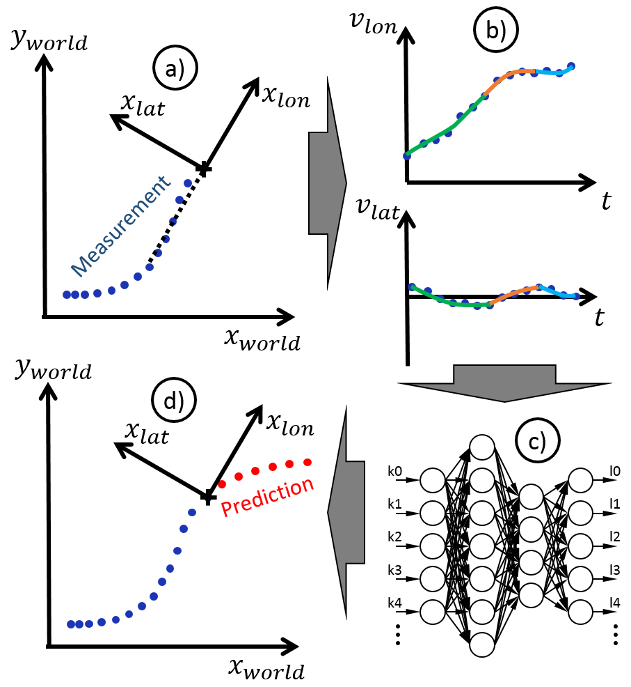
Figure 2: Overview of the proposed path prediction method.

III-C Multilayer Perceptron for Prediction

We apply an MLP to predict the motion state and/or the future trajectory of the VRU based on the extracted patterns (see Fig. 2 c). The MLP provides high flexibility and efficiency for the given application as it allows predicting multiple output dimensions at the same time. The applied artificial neural network consists of neurons with sigmoid activation functions, whereas other configurations (identity, Gaussian) were evaluated, too. After normalizing the input patterns using a $z$-transformation, a training is performed with the Resilient Backpropagation (RPROP) algorithm [26]. The number and sizes of the hidden layers are variable and also part of the optimization process.

III-D Recognition of Motion State

For the recognition of the motion state, a model of the four states Waiting, Starting, Moving, and Stopping is used. This basically allows the 8 (out of a possible basic quantity of 12) state transitions depicted in Fig. 3, as the transitions between Waiting and Moving are always separated by one of the transition states Starting or Stopping.

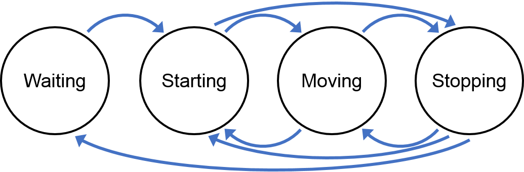
Figure 3: Modeled motion states and physically possible state transitions.

For the online classification, an MLP output layer with 4 neurons, one representing each state, is configured. The trajectories used for training are labeled with a distinct class label for every element, generating output training patterns with a one at the element representing the current ground truth class and zeros at all others. No further measures are taken to define physically meaningful transitions or transition probabilities explicitly, as the neural network should be given the possibility to learn these aspects from scratch without further conditions. With this approach, the trained classifier provides a pseudo-probabilistic rating for each state. As the four output neurons have no direct interconnection the cumulative probability is not explicitly specified to 100%, so an additional scaling step has to be applied if this output information is needed by the subsequent application.

III-E Prediction of Trajectory

To predict the VRU trajectory, we use a representation according to the one of the input patterns. To train the predictor, again characteristic time series are extracted from the ground truth trajectory within a certain time window (cf. Section III-A) and the time series are approximated using orthogonal basis polynomials to get a low-dimensional representation independent of the cycle time (cf. Section III-B). The choice of the MLP output pattern is completely independent of the one of the input pattern, what allows different time series and polynomial degrees. Each polynomial coefficient is estimated by a separate MLP output neuron, where also a $z$-transformation is used for normalization. During online application, the process is performed vice versa: The output pattern predicted by the MLP is transformed back and the time series is evaluated at the requested discrete points of time. It is then transformed to an estimation of the future trajectory in the original global coordinate system using the current VRU position and movement direction (see Fig. 2 d).

III-F State Specific Trajectory Prediction

After training, the weights of the MLP implicitly contain the knowledge of the trained movements (starting, stopping, etc.) within a single model. Besides this monolithic approach, a second approach combining state classification with several specifically trained models for trajectory prediction is implemented and evaluated. The architecture of the prediction system using the PolyMLP method is shown in Fig. 4.

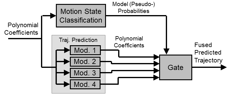
Figure 4: Motion state specific trajectory prediction.

The measured trajectory is fed into a classifier module that predicts the current motion state as described in Sec. III-D (Recognition of Movement State). In parallel, the trajectory is fed into several (here: four) PolyMLP modules for trajectory prediction. Each predictor is specifically trained with scenes containing movements according to one output of the classifier model, i.e. motion state. As the prediction modules can use the same configuration for preprocessing the trajectory and polynomial approximation, only the output of the specifically trained MLPs has to be processed separately. The predicted polynomial coefficients are fed into a gating module and added as weighted sum based on the class posterior probabilities. Finally, the resulting fused coefficient set is used to generate the final trajectory prediction. This method of explicit separation of classification and trajectory prediction has the advantage that the classification as well as the prediction modules can be replaced by other approaches. For our evaluation we are thus able to use the MCHOG/SVM approach within the classification module or physical starting and stopping models in the prediction module as comparison techniques.

IV Test Sites and Data Sets

For training, optimization, and evaluation of the models, appropriate databases containing realistic VRU data play an essential role. We use an urban traffic intersection in order to gain measurements of realistic, unaffected pedestrian and cyclist behavior under real conditions. The observed area includes two sidewalks, two crosswalks and a bicycle lane which is separated from the motor vehicle lanes by road markings (see Fig. 5).

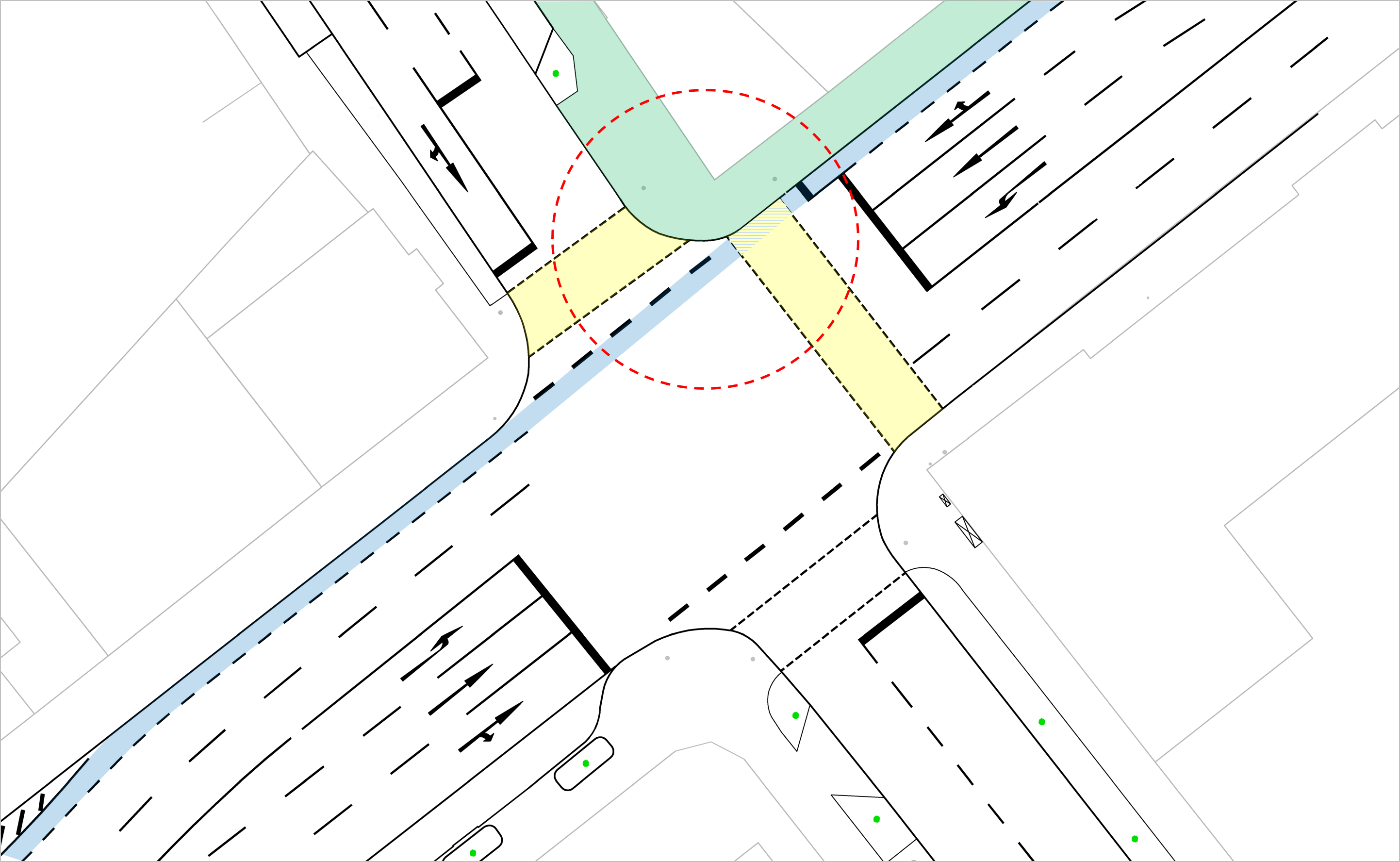
Figure 5: Map of the public intersection used to acquire VRU behavior data. The area highlighted in green represents the observed sidewalk, the yellow areas the crosswalks. The bicycle lane is highlighted in blue. The area of overlapping fields of view of the high resolution cameras allowing high-precision 3D position measurements is marked by the red circle.

The intersection is equipped with eight low-resolution (640 x 480 px) and two high-resolution (1920 x 1080 px) grayscale cameras, as well as 14 eight-layer laser scanners. All sensors are mounted on infrastructure elements, e. g., street lamps and traffic light posts, in heights between 4 and 11 meters in order to reduce the risk of occlusions. The sensor system is described in detail in [27]. The high-resolution cameras are pointing towards a part of the intersection where two crosswalks meet and therefore a high quantity of pedestrians is expected (Fig. 5, dashed red circle). They form a wide angle stereo system allowing precise 3D measurements with an accuracy better than 3 cm for corresponding image points. The laser scanners cover the central intersection and the area of three approaching roads up to 100 m. They provide object point clouds and are used to track cyclists in a larger area beyond the stereo range of the camera system. The low resolution cameras are currently only used for manual scene observation and the labeling of movement phases.

Fig. 6 shows the framework for the extraction of pedestrian and cyclist head trajectories from stereo video data. At the first stage, both synchronous camera frames are individually scanned by a sliding-window histogram of oriented gradients (HOG) pedestrian detector [28]. The upper half of the detection rectangles serve as region of interest (ROI) for the head detectors , which are based on Haar [29] and local binary pattern (LBP) features [30]. In the next step, the most likely head position in pixel coordinates is determined fusing HOG, Haar, and LBP detections. If the head position is already tracked, template matching is used as a fourth measurement value that is fed into the fusion module. The tracked head positions from both cameras are merged to 3D world coordinate positions via triangulation. In a final step, valid positions are connected to 3D trajectories and stored.

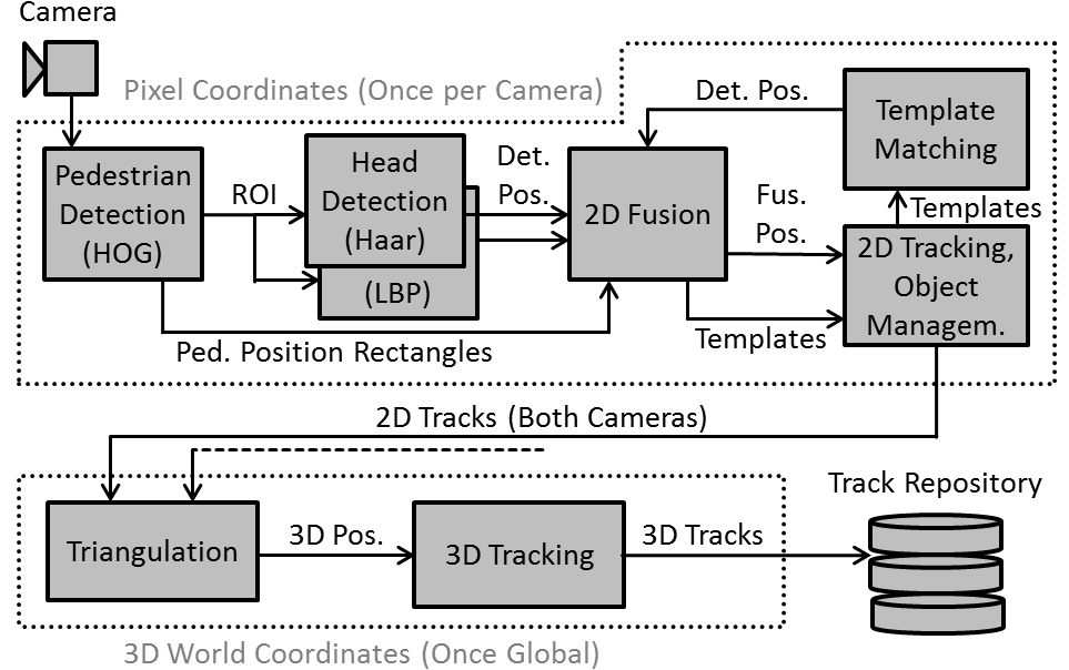
Figure 6: Framework for extraction of trajectories.

IV-A Full Pedestrian Dataset

The Full Pedestrian Dataset contains 1068 scenes of pedestrians with 4 to 10 seconds length recorded by the high resolution stereo system with a sample rate of 50 Hz. The scenes are categorized with one of the following scene labels (the number in brackets indicates the number of scenes):

• Moving scenes (288) contains pedestrians crossing the observed area without stopping or significant deceleration, including scenes of walking along the sidewalk, crossing one of the roads, walking straight ahead or making a turn.

• Waiting scenes (259) contains pedestrians standing at the sidewalk, mostly waiting for a green pedestrian light signal (head velocity lower than 0.3 m/s).

• Starting scenes (336) contains pedestrians accelerating from standing position. These scenes also contain up to 3 seconds before and after the actual acceleration phase if available within the data.

• Stopping scenes (185) contains scenes where moving pedestrians decelerate to standstill. These scenes also contain up to 3 seconds before and after the actual deceleration phase.

The Starting scenes include time labels of the start, and if existent within the scene, also of the end of the acceleration phase. The start is determined as the time where the ground truth head velocity exceeds 0.2 m/s, its end is labeled at the first local maximum after the velocity exceeds 80% of their steady state value. The labeling of Stopping is done vice versa. Table I gives an overview over the training and test scenes and extracted patterns (combination of predictor in- and output, generated for each time cycle with complete in- and output time window around).

TABLE I: Training- and test data in the Full Pedestrian Dataset. The table shows the number of scenes used and of the according extracted patterns in brackets.

	Waiting	Starting	Moving	Stopping
Train	177 (54.6 k)	239 (66.5 k)	201 (45.2 k)	130 (42.6 k)
Test	82 (25.3 k)	97 (25.1 k)	87 (20.1 k)	55 (17.7 k)
Total	259 (79.8 k)	336 (91.6 k)	288 (65.3 k)	185 (60.3 k)

IV-B Detailed Pedestrian Dataset

The Detailed Pedestrian Dataset is an extended subset of 136 Starting, 107 Stopping, and 69 Moving scenes from the full set with finer differentiated ground truth motion states. It contains manually determined labels by video data observation, e. g., the state, the timestamps of heel-off, the first and second heel-down, the entering of the roadway and partial occlusions.

IV-C Cyclist Dataset

The Cyclist Dataset contains 494 trajectories of bicyclists including 86 Moving, 133 Waiting, 197 Starting and 78 Stopping scenes. As the cyclists’ phases of acceleration and deceleration typically take more time and distance as those of pedestrians, the laser scanner system was used to capture also tracks leaving the more limited common field of view of the high resolution stereo cameras. In return, a lower spatial and temporal resolution was accepted for those tracks.

As well the pedestrian as the cyclist dataset with labeled head trajectories is available to the scientific community [31].

V Experiments and Results

V-A Training and Optimization

The training and optimization of the pedestrian models is performed using the training split (747 scenes) of the Full Pedestrian Database. The training scenes are split again into 70% for the MLP training with RPROP and 30% as validation set for the optimization of the meta parameters (pre-filtering parameters, sliding window positions and sizes, polynomial representation). The target function of the MLP training is a minimization of the mean squared error (MSE) of the $z$-normalized output, while the meta parameters are optimized regarding a maximum accuracy (state classification) and a minimum average specific average Euclidean error (ASAEE, see Sec. V-D). For the selection of the input time series representation (Sec. III-A) a five-fold cross validation within the training set is applied.

The results show that the time series of the 2D velocity in the pedestrians ego system perform best as basis for the input patterns of both state classification and trajectory prediction, while only decent differences to other tested representations (see Sec. III-A) were observed (0% – 3% for state clas., 3% – 9% for traj. pred.). The representation with polynomials shows slight advantages compared to the direct input of each time series (0% – 5%). The final outcome of the optimization of the sliding window and polynomial configuration are two consecutive time windows of 800 ms and 200 ms length with polynomial degrees of 3. For the output pattern of the trajectory prediction, the time series of the 2D position in the ego system with five consecutive sliding windows (500 ms each, polynomial degree 2) is used, leading to an overall prediction time horizon of 2.5 s.

V-B Motion State Classification

In the first experiment, the quality of the proposed method for motion state classification is evaluated. For comparison, an IMM-KF using CP/CV models and the directly video-based method MCHOG/SVM [23] are applied to the same scenes. As the evaluation requires the additional labels of the Detailed Pedestrian Dataset (i.e. the time of heel-off to distinguish between standing and starting phase), the following tests are performed using these patterns. In the experiment, the overall quality of the different motion state classifiers is evaluated by means of the accuracy (ACC) and the F₁ score.

As the quality measures and both comparison methods only support binary classification, the ground truth label Waiting is assigned to timestamps before and the label Moving to those during and after the manually determined heel-off within the 40 Starting scenes. Two PolyMLP predictors are trained: The first uses a four-classes output and a binarization after the prediction step by thresholding the sum probability $P_{\text{Sum}}$ of the three estimates for Starting, Moving and Stopping: $P_{\text{Sum}}=P(\text{Start})+P(\text{Mov})+P(\text{Stop})$. The second is directly trained with this two-class split and uses a single output neuron to predict $P_{\text{Sum}}$ while the class Waiting is defined by the complement probability $1-P_{\text{Sum}}$. The 35 Stopping scenes are also tested with a four-class model, where a threshold on $P_{\text{Sum}}=P(\text{Stop})+P(\text{Wait})$ is used for binarization. The two-class model is again trained directly with this split and predicts the output with a single neuron. As the classifier quality measures are depending on the binarization threshold, the optimal value is chosen by maximization of the accuracy on the training data (an optimization of the F₁-score leads to the same operating point). The resulting quality measures of both test scene types using optimal bias values are shown in Table II.

TABLE II: Accuracy (ACC) and F₁ score of the classifiers for the 40 starting and 35 stopping test scenes of the detailed pedestrian database.

	Start		Stop
	ACC	F1	ACC	F1
IMM-KF	0.9803	0.9565	0.9248	0.9548
PolyMLP (4 Cl.)	0.9819	0.9601	0.9381	0.9644
PolyMLP (2 Cl.)	0.9824	0.9612	0.9363	0.9636
MCHOG	0.9844	0.9659	0.9141	0.9503

For the regarded Starting scenes, the quality measures show only minor differences with slight advantages for MCHOG and slight disadvantages for the IMM-KF compared to PolyMLP. Clearer differences can be observed for the Stopping scenes: Here, PolyMLP performs best, while IMM-KF outperforms MCHOG. The optimization thereby results in a relatively high threshold for the CV model probability $P_{\text{CV}}$ of the IMM-KF of 98.9%, which means that stopping can be recognized in an early state.

As the PolyMLP method performs a multi-class prediction of all four motion states, it is additionally evaluated using the 321 test tracks of the Full Pedestrian Dataset. The result shows an accuracy of 88.6%, which is lower than the one of the Detailed Pedestrian Dataset as the classifier has now to distinguish between Starting, Walking, and Stopping, too. More detailed results are set out in the confusion matrix in Table III which shows an obvious substantial asymmetry of the classification rates of the four types of movement.

TABLE III: Confusion matrix for the classification of the motion state. The rows contain the specific ground truth label. The columns contain the percentage of detections with regard to the total number of patterns of the ground truth label (sum of every row equals 100%).

	Waiting	Starting	Walking	Stopping
Waiting	98.6%	0.7%	0.0%	0.7%
Starting	11.8%	77.1%	8.8%	2.3%
Walking	2.0%	4.8%	88.1%	5.0%
Stopping	2.1%	2.2%	34.8%	60.9%

The state Waiting can be separated best from the three others, leading to a correct classification rate of 98,6%. Most challenging is the transition from Walking to Stopping: Here, especially the begin of the stopping phase is difficult to distinguish from velocity variations during walking, crossing one of the roads, or bending in.

V-C Early Recognition of State Transitions

For an evaluation of the prediction model ability to early recognize state transitions, the temporal development of the classification quality depending on the binarization threshold is analyzed. Here, the trade-off between the classifier’s sensitivity leading to short reaction times on movement transitions on the one hand and low false alarm rates on the other hand should be examined. For this purpose, the Detailed Pedestrian Dataset is evaluated scene-wise on false positives under variation of the chosen threshold value. A scene is already considered as false positive if the classifier produces one false positive output at any single time step. Under that condition, the quality measures of the precision and the F₁ score can be evaluated depending on the threshold. The additional determination of the accuracy does not make sense here as the number of true negatives is zero for most of the possible values (The state transition is detected earlier or later in any case.). Furthermore, the mean time for the correct classification of the movement transition relative to the according manually labeled point in time is determined. For this evaluation, only scenes without false positives for the regarded threshold value are considered. Fig. 7 shows the four quality measures evaluated on the Starting scenes dependent on the chosen threshold for the PolyMLP and the MCHOG/SVM classifier.

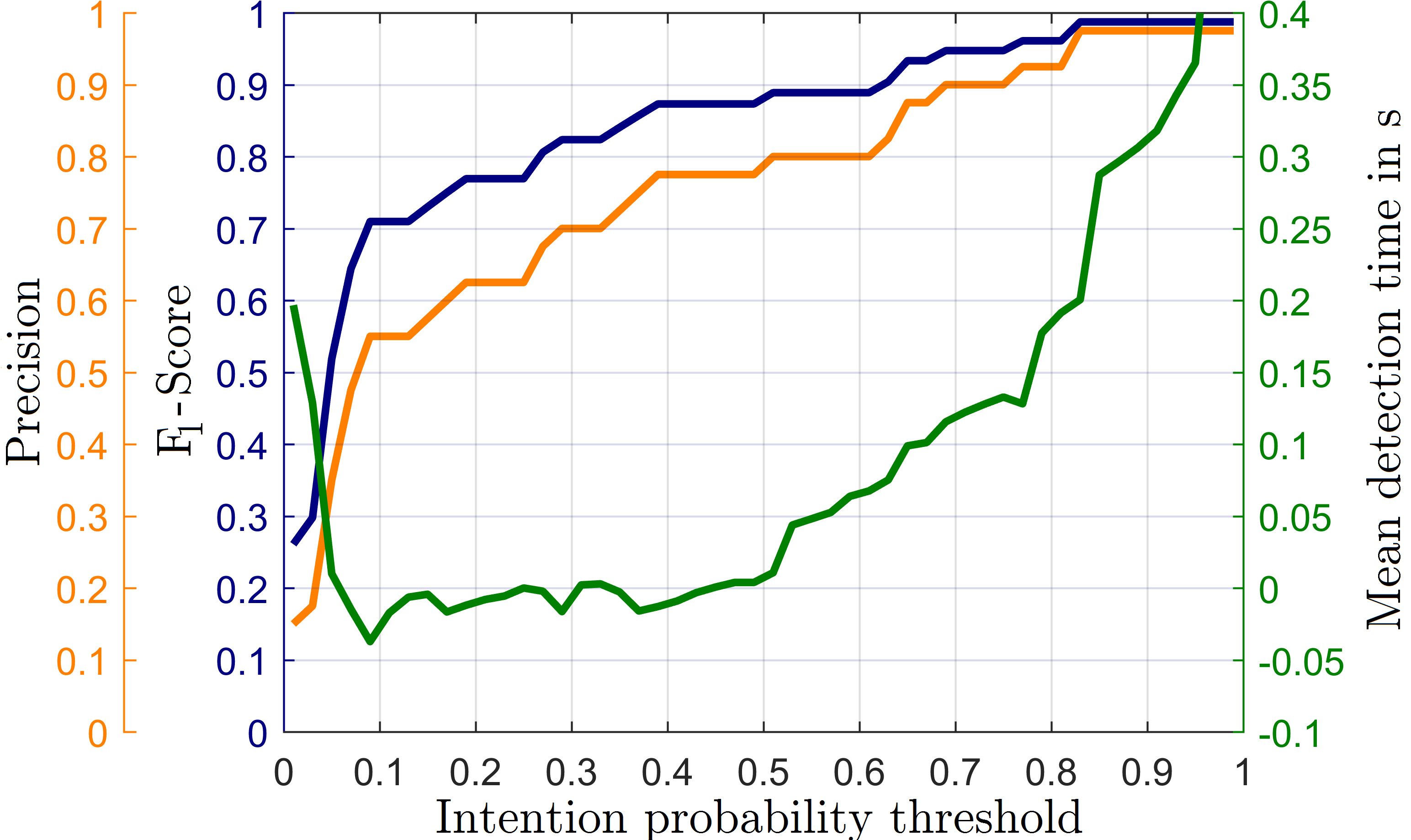
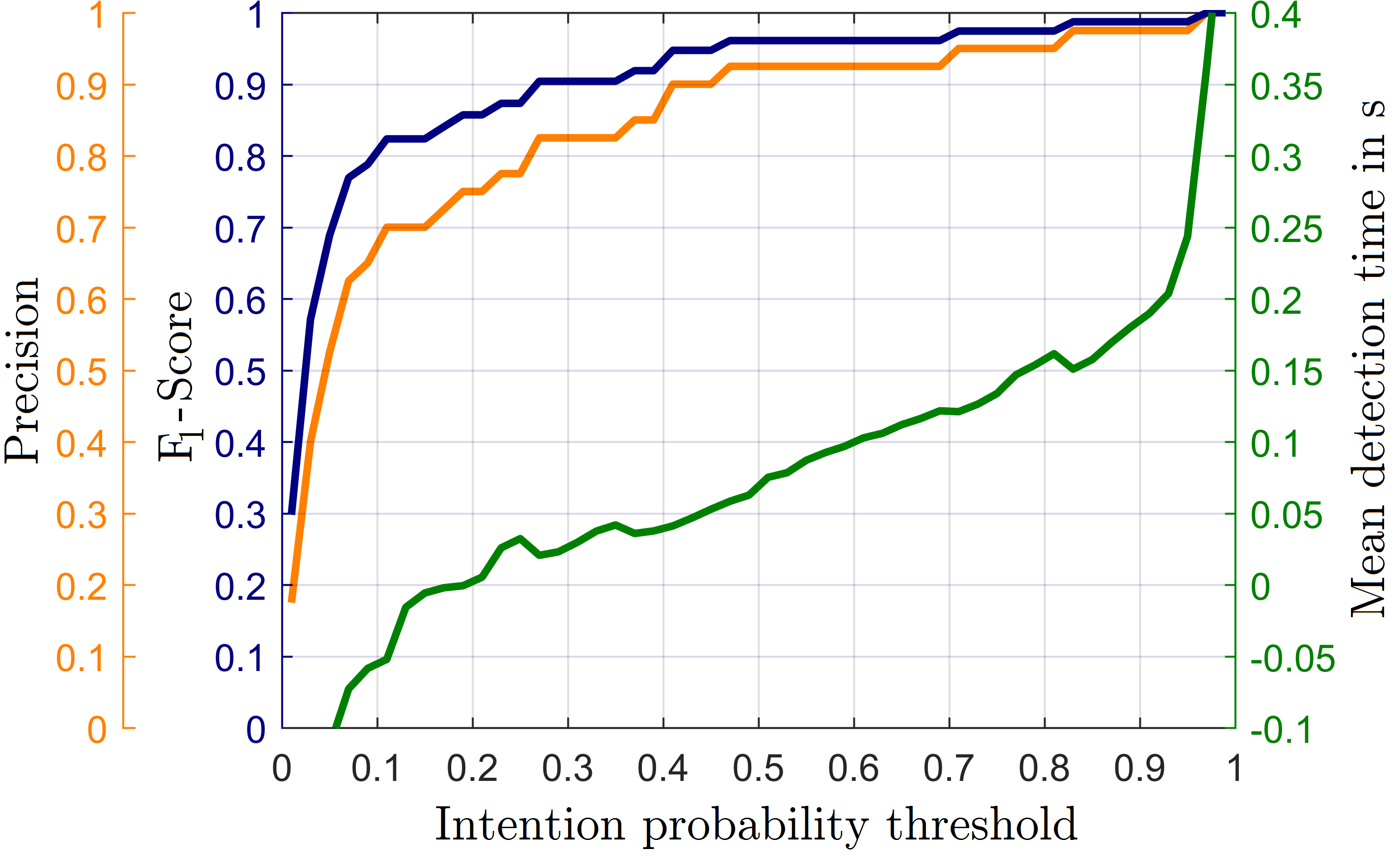
Figure 7: Evaluation of the recognition of starting movements using 40 scenes of the Detailed Pedestrian Dataset for PolyMLP (upper plot) and MCHOG (lower plot). The plots show the precision (orange), the F₁-score (blue) and the mean time needed for detection of the starting motion relative to the manually labeled time of the heel-off (green). The chosen threshold on the pseudo probabilistic classifier output is drawn on the horizontal axis.

The results show that an F₁ score of 95% and a precision of 90% are reached 130 ms after the labeled heel-off. The MCHOG classifier is about 3 frames faster at the same operating point, and thus able to detect the starting motion about 70 ms earlier. In contrast, the IMM-EKF needs 160 ms (plot not shown).

Fig. 8 shows the plots for the same kind of evaluation regarding the recognition of stopping motion. Here, the detection time is measured in relation to the heel-down of the last step.

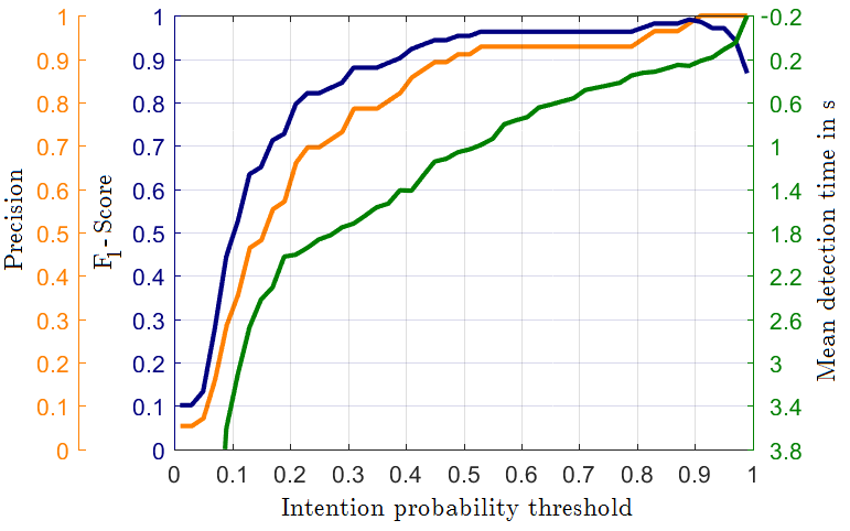
Figure 8: Evaluation of the recognition of stopping movements using 35 test scenes of the Detailed Pedestrian Dataset for PolyMLP (upper plot) and MCHOG (lower plot). The axes and plot configuration correspond to Fig. 7.

In this case, the PolyMLP method performs best, reaching an F₁ score of 95% and a precision of 90% already 1.4 s before the heel-down (on average). Both other classifiers, MCHOG/SVM and IMM-KF, reach this quality level only 400 ms later, which is a large time span in the field of active accident prevention.

Actually, we want to reach 100% F₁ score and precision, but there is a tradeoff between F₁/precision and mean detection time and sometimes we are not able to get at 100% F₁/precision. Therefore, we choose the 95% F₁ and 90% precision levels for comparison of the PolyMLP and the MCHOG/SVM classifier on starting motions (Fig. 7) and stopping motions (Fig. 8). When analyzing accidents it was shown that an initiation of an emergency break 160 ms earlier at a Time-to-Collision of 660 ms and a vehicle speed of 50 km/h reduces the probability of an injury resulting in a hospital stay from 50% to 35% [7]. This underlines the need for detecting basic movements as early as possible and that some milliseconds can make the difference. Fig. 7 shows that for an F₁ score/prediction of 100% some starting motions can only be detected 0.4 sec or later after heel off. This indicates that there is still research to be done.

V-D Generally Applicable Methods of Trajectory Prediction

In this section, the generally applicable methods of trajectory prediction, the monolithic and the two-stage specific PolyMLP, are evaluated and compared to CV Kalman filtering as baseline. As performance measure, the average specific average Euclidean error

$$\text{ASAEE}=\frac{1}{N}\sum\limits_{i=1}^{N}\frac{\text{AEE}(t_{pred}(i))}{t_{pred}(i)}$$ (2)

with the AEE being the average Euclidean position error for a specific time span $t_{pred}(i)$, the index $i$ and the total number $N$ of discrete time spans predicted into the future (see [20]). In our case, $N$ = 125 steps with $t_{pred}$ = 0.02 .. 2.50 s are used. The ASAEE is evaluated separately for the methods and the four scene types within the Full Pedestrian Dataset, leading to the results shown in Table IV.

The results of the Kalman Filter already show the varying degrees of difficulty of the single scene types: As expected, Waiting generates the lowest errors (7.8 cm/s). The ASAEE rises with increasing presence of velocity changes resulting in the further order Walking, Stopping, and Starting. Starting includes the most abrupt velocity changes in combination with the absence of a defined direction regarding the trajectory at the beginning of the movement.

TABLE IV: ASAEE (in cm/s) of universally applicable prediction methods for the four scene classes in comparison. The table shows the results for CV Kalman Filtering (CV-KF), the single stage (monolothic) MLP model (PolyMLP), the two-stage MLP model (PolyMLP (2 St.)) and the combination of the ground truth class labels with the specifically trained PolyMLP models (GT+PolyMLP).

	Waiting	Starting	Walking	Stopping	Mean
CV-KF	7.8	44.2	27.6	33.5	28.3
PolyMLP	6.9	33.6	25.5	22.7	22.2
PolyMLP (2 St.)	4.7	34.4	23.4	25.2	21.9
GT+PolyMLP	3.9	32.3	22.8	22.5	20.4

For Waiting and Walking, the monolithic PolyMLP shows moderate improvements of 12% and 8% to the Kalman Filter. The improvement for scenes including movement transitions is substantially larger: Starting scenes improve by 24%, Stopping scenes even by 32%. Considering only the predictions directly within the labeled actual transition phase, an improvement of 42% (Starting) resp. 43% (Stopping) can be observed.

In comparison to the monolithic PolyMLP, the two-stage approach shows a slight further improvement of 1 – 2 cm/s on Waiting and Walking scenes while the error for Starting and Stopping increases by approximately the same values. This means that the additional classification error outweighs the improvement of the specific trajectory prediction models for the transition scenes. Overall, the two-stage model leads to slightly lower errors, whereas the difference is only 1% considering the average of the four scene class results and 3% considering the ASAEE evaluated over all test patterns.

In order to examine the maximum potential of the two-stage approach, the classification stage is replaced by the ground truth class labels. Thus, the trajectory prediction stage is always able to choose the optimal model. The experimental results show a potential limit at a 7% lower average scene class error. Considering the separate scene types, especially the Starting and Stopping prediction of the monolithic model already performs very close to the optimum.

V-E Two-stage Trajectory Prediction

In this test series, the quality of the motion specific two-stage trajectory prediction methods for Starting and Stopping scenes are evaluated and compared to the generally applicable methods tested in the previous section using the Detailed Pedestrian Database. We evaluate the predictions only during the labeled movement transition, as the dataset contains longer phases of waiting resp. walking before the starting resp. the stopping movement. The third scene class Moving is included in order to evaluate the sensitivity for false alarm stopping classifications.

The results presented in Table V show the superiority of the machine learning models compared to the prediction of the (generally optimized) CV Kalman Filter. The application of the monolithic PolyMLP model leads to a reduction of the prediction error by 36.5% for Starting and 40.7% for Stopping scenes. As shown in the last row of the table by combining the ground truth classification with the specifically trained PolyMLP prediction, the potential for improvement by two-stage modeling is only 4.9% for Starting, but 11.0% for Stopping scenes. As classification stage we evaluated the four-class PolyMLP classifier already tested on the Full Pedestrian Dataset (PolyMLP) and the image-based two-class MCHOG/SVM classifiers (MCHOG). For trajectory prediction, specifically trained PolyMLP models and physically based models for starting and stopping (PhysMod) are evaluated. In the case of Starting, the specific PolyMLP models outperform the physical model by 9% while they perform almost equal on Stopping motions. A distinct disadvantage of the physical Stopping model thereby is its sensitivity on false alarms of the classifier stage, leading to a particularly high prediction error on Moving scenes. Considering the machine learning models, it is remarkable that no two-stage approach is able to outperform the single-stage PolyMLP. While with Starting scenes no substantial differences between the single-stage PolyMLP and the two-stage models with PolyMLP- and MCHOG classification are measured, the monolithic approach slightly outperforms both at Stopping by 6.4% resp. 3.7%.

TABLE V: ASAEE (in cm/s) of the different optimized trajectory prediction methods for the three scene classes in comparison.

	Starting	Stopping	Moving
KF	49.94	36.04	23.35
PolyMLP	31.71	21.37	22.41
PolyMLP+PhysMod	35.23	21.75	41.97
PolyMLP+PolyMLP	31.54	22.84	23.10
MCHOG+PolyMLP	31.85	22.20	22.72
GT+PolyMLP	30.17	19.01	21.43

V-F Cyclists

For the Cyclist Dataset, the applicability of the PolyMLP concept to this VRU type could also be shown. As typical cyclist velocities at the test intersection are 2 – 3 times higher than those of pedestrians, their reach within the prediction horizon is much larger. Thus, the position prediction errors rise, here by 51% for Starting and for 79% on Stopping scenes compared to the Full Pedestrian Database. The fundamental insights to those gained for pedestrians: Especially regarding Starting scenes, the PolyMLP model could outperform an optimized CV-KF by 46%. Here, also physical modeling already leads to an improvement of 27% compared to CV-KF. A significant advantage (34%) of PolyMLP is also observed on stopping scenes, while the Kalman Filter prediction was not improved on Waiting ($\pm$0%) and Moving scenes (-11%). For a more detailed evaluation on the cyclist dataset, see [21].

V-G Processing Time

Another important aspect is the computational time for training and for the online application of the predictor. As the dimensionality of the in- and output features is relatively low due to the polynomial representation, the training time of the MLP also remains short. Using a current desktop PC (Intel Core i7-3770, 4 $\times$ 3.4 GHz, 8 GB RAM), 12 min are needed for the single stage PolyMLP model, while 97% of the final prediction quality is already reached after approx. 1 min.

For the two-stage approach, the preprocessing and the polynomial approximation step have only to be performed once as long as the same polynomial configuration is used for all models included. With regard to the one-stage approach, the computation time rises by only 35% to 70 $\mu$s. Altogether the algorithms perform very efficient with computational times several orders of magnitude lower than, e. g., most techniques of pedestrian or cyclist detection. The used algorithms of video-based head detection and tracking, e. g., are processed within less than 40 ms on the test system. Therefore, a HOG/SVM pedestrian detector processing full-frames on the GPU in order to deliver ROIs for the head detection is the limiting factor.

VI Conclusion and Future Work

In this article we proposed VRU movement models based on machine learning methods. The presented approach uses the measured VRU trajectory to predict the current motion state and the future trajectory. It is compared to CV- and IMM-Kalman-Filtering, physically based models for starting and stopping and video-based motion classification with a MCHOG descriptor and SVMs. The results show that PolyMLP clearly outperforms Kalman Filtering for classification and trajectory prediction, in particular in the cases of starting and stopping motions. Physical models perform also better than KF, but are outperformed by PolyMLP too, especially considering the handling of false positive classifications. MCHOG/SVM uses additional image-based information as input and thus shows slightly more reliable early detection of starting motion (70 ms faster on avrg.), but is approx. 400 ms slower at the classification of stopping. The two-stage approach of motion state classification and trajectory prediction did not lead to a significant further improvement of the prediction quality in our case, but reveals the potential to include other classification of prediction models, perhaps basing on complementary sensors. Altogether, PolyMLP represents a promising method for intention recognition of VRUs with state-of-the-art prediction quality and a high degree of flexibility with regard to VRU type, used sensor system, predicted time horizon and the concrete field of ADAS application.

Our future work comprises the further evaluation of the techniques using on-board sensors in a moving vehicle under various traffic conditions. Here, especially the handling of measurement noise and the vehicle’s ego motion represent additional challenges. Another promising approach is the inclusion of additional information, e. g. from high-precision maps, other on-board sensors, infrastructure knots or vehicles via V2I or V2V communication.

Michael Goldhammer received the M. Eng. degree in Electrical Engineering and Information Technology from the University of Applied Sciences Aschaffenburg (Germany) in 2009 and the Dr. rer. nat. degree in computer sciences in 2016 from the University of Kassel (Germany). His PHD thesis focuses on self-learning algorithms for video-based intention detection of pedestrians. His research interests include machine vision and self-learning methods for sensor data processing and automotive safety purposes.

Sebastian Köhler received the Dipl.-Ing. (FH) degree in Mechatronics and the M. Eng. degree in Electrical Engineering and Information Technology from the University of Applied Sciences Aschaffenburg, Germany, in 2010 and 2011, respectively. Currently, he is working on his PhD thesis in cooperation with the Institute of Measurement, Control, and Microtechnology, University of Ulm, Germany, focussing on intention detection of pedestrians in urban traffic. His main research interests include stereo vision, sensor and information fusion, road user detection and short-term behavior recognition for ADAS.

Stefan Zernetsch received the B.Eng. and the M.Eng. degree in Electrical Engineering and Information Technology from the University of Applied Sciences Aschaffenburg, Germany, in 2012 and 2014, respectively. Currently, he is working on his PhD thesis in cooperation with the Faculty of Electrical Engineering and Computer Science of the University of Kassel, Germany. His research interests include cooperative sensor networks, sensor data fusion, multiple view geometry, pattern recognition and short-term behavior recognition of traffic participants.

Konrad Doll received the Diploma (Dipl.-Ing.) degree and the Dr.-Ing. degree in Electrical Engineering and Information Technology from the Technical University of Munich, Germany, in 1989 and 1994, respectively. In 1994 he joined the Semiconductor Products Sector of Motorola, Inc. (now Freescale Semiconductor, Inc.). In 1997 he was appointed to professor at the University of Applied Sciences Aschaffenburg in the field of computer science and digital systems design. His research interests include intelligent systems, their real-time implementations on platforms like CPU, GPUs and FPGAs and their applications in advanced driver assistance systems. Konrad Doll is member of the IEEE.

Bernhard Sick received the diploma, the Ph.D. degree, and the ”Habilitation” degree, all in computer science, from the University of Passau, Germany, in 1992, 1999, and 2004, respectively. Currently, he is full Professor for intelligent embedded systems at the Faculty for Electrical Engineering and Computer Science of the University of Kassel, Germany. There, he is conducting research in the areas autonomic and organic computing and technical data analytics with applications in biometrics, intrusion detection, energy management, automotive engineering, and others. He authored more than 90 peer-reviewed publications in these areas. Dr. Sick is associate editor of the IEEE TRANSACTIONS ON CYBERNETICS. He holds one patent and received several thesis, best paper, teaching, and inventor awards. He is a member of IEEE (Systems, Man, and Cybernetics Society, Computer Society, and Computational Intelligence Society) and GI (Gesellschaft fuer Informatik).

Klaus Dietmayer was born in Celle, Germany in 1962. He received the Diploma degree (equivalent to M.Sc. degree) in electrical engineering from Braunschweig University of Technology, Braunschweig, Germany, in 1989 and the Dr.-Ing. degree (equivalent to Ph.D. degree) from the Helmut Schmidt University, Hamburg, Germany, in 1994. In 1994, he joined the Philips Semiconductors Systems Laboratory, Hamburg, as a Research Engineer. Since 1996, he has been a Manager in the field of networks and sensors for automotive applications. In 2000, he was appointed to a professorship at Ulm University, Ulm, Germany, in the field of measurement and control. He is currently a Full Professor and the Director of the Institute of Measurement, Control and Microtechnology with the School of Engineering and Computer Science, Ulm University. His research interests include information fusion, multiobject tracking, environment perception for advanced automotive driver assistance, and E-Mobility. Dr. Dietmayer is a member of the German Society of Engineers VDI/VDE.

References

- [1] Global Status Report on Road Safety 2015. World Health Organization, 2015.
- [2] Y. Bar-Shalom, X. R. Li, and T. Kirubarajan, Estimation with Applications to Tracking and Navigation: Theory Algorithms and Software. John Wiley and Sons, 2001.
- [3] M. Bertozzi, A. Broggi, A. Fascioli, A. Tibaldi, R. Chapuis, and F. Chausse, “Pedestrian localization and tracking system with kalman filtering,” in IEEE Intelligent Vehicles Symposium (IV), 2004, pp. 584–589.
- [4] E. Binelli, A. Broggi, A. Fascioli, S. Ghidoni, P. Grisleri, T. Graf, and M. Meinecke, “A modular tracking system for far infrared pedestrian recognition,” in IEEE Intelligent Vehicles Symposium (IV), 2005, pp. 759–764.
- [5] M. Meuter, U. Iurgel, S. Park, and A. Kummert, “The unscented kalman filter for pedestrian tracking from a moving host,” in IEEE Intelligent Vehicles Symposium (IV), 2008, pp. 37–42.
- [6] N. Schneider and D. Gavrila, “Pedestrian path prediction with recursive bayesian filters: A comparative study,” in Pattern Recognition, ser. Lecture Notes in Computer Science. Springer, 2013, vol. 8142, pp. 174–183.
- [7] C. Keller, C. Hermes, and D. Gavrila, “Will the pedestrian cross? probabilistic path prediction based on learned motion features,” in Pattern Recognition, ser. Lecture Notes in Computer Science. Springer, 2011, vol. 6835, pp. 386–395.
- [8] C. F. Wakim, S. Capperon, and J. Oksman, “A markovian model of pedestrian behavior,” in International Conference on Systems, Man and Cybernetics, vol. 4, 2004, pp. 4028–4033.
- [9] C. Keller and D. Gavrila, “Will the pedestrian cross? a study on pedestrian path prediction,” IEEE Transactions on Intelligent Transportation Systems, vol. 15, no. 2, pp. 494–506, 2014.
- [10] R. Quintero, J. Almeida, D. F. Llorca, and M. A. Sotelo, “Pedestrian path prediction using body language traits,” in IEEE Intelligent Vehicles Symposium (IV), 2014, pp. 317–323.
- [11] R. Quintero, I. Parra, D. F. Llorca, and M. A. Sotelo, “Pedestrian path prediction based on body language and action classification,” in IEEE International Conference on Intelligent Transportation Systems (ITSC), 2014, pp. 679–684.
- [12] A. T. Schulz and R. Stiefelhagen, “Video-based pedestrian head pose estimation for risk assessment,” in International IEEE Conference on Intelligent Transportation Systems (ITSC), 2012, pp. 1771 –1776.
- [13] ——, “Pedestrian intention recognition using latent-dynamic conditional random fields,” in IEEE Intelligent Vehicles Symposium (IV), 2015, pp. 622–627.
- [14] ——, “A controlled interactive multiple model filter for combined pedestrian intention recognition and path prediction,” in IEEE International Conference on Intelligent Transportation Systems (ITSC), 2015, pp. 173–178.
- [15] J. Kooij, N. Schneider, F. Flohr, and D. Gavrila, “Context-based pedestrian path prediction,” in European Conference on Computer Vision (ECCV), 2014, pp. 618–633.
- [16] M. Goldhammer, M. Gerhard, S. Zernetsch, K. Doll, and U. Brunsmann, “Early prediction of a pedestrian’s trajectory at intersections,” in International IEEE Conference on Intelligent Transportation Systems (ITSC), 2013, pp. 237–242.
- [17] M. Goldhammer, A. Hubert, S. Koehler, K. Zindler, U. Brunsmann, K. Doll, and B. Sick, “Analysis on termination of pedestrians’ gait at urban intersections,” in IEEE International Conference on Intelligent Transportation Systems (ITSC), 2014, pp. 1758–1763.
- [18] M. Goldhammer, K. Doll, U. Brunsmann, A. Gensler, and B. Sick, “Pedestrian’s trajectory forecast in public traffic with artificial neural networks,” in International Conference on Pattern Recognition (ICPR), 2014, pp. 4110–4115.
- [19] M. Goldhammer, S. Köhler, K. Doll, and B. Sick, “Camera based pedestrian path prediction by means of polynomial least-squares approximation and multilayer perceptron neural networks,” in SAI Intelligent Systems Conference (IntelliSys), 2015, pp. 390–399.
- [20] M. Goldhammer, S. Köhler, K. Doll, and B. Sick, Track-Based Forecasting of Pedestrian Behavior by Polynomial Approximation and Multilayer Perceptrons. Springer International Publishing, 2016, pp. S. 259–279. [Online]. Available: http://dx.doi.org/10.1007/978-3-319-33386-1_13
- [21] S. Zernetsch, S. Kohnen, M. Goldhammer, K. Doll, and B. Sick, “Trajectory prediction of cyclists using a physical model and an artificial neural network,” in 2016 IEEE Intelligent Vehicles Symposium (IV), 2016, pp. 833–838.
- [22] S. Köhler, M. Goldhammer, S. Bauer, S. Zecha, K. Doll, U. Brunsmann, and K. Dietmayer, “Stationary detection of the pedestrian’s intention at intersections,” IEEE Intelligent Transportation Systems Magazine, vol. 5, no. 4, pp. 87–99, 2013.
- [23] S. Köhler, M. Goldhammer, K. Zindler, K. Doll, and K. Dietmayer, “Stereo-vision-based pedestrian’s intention detection in a moving vehicle,” in IEEE International Conference on Intelligent Transportation Systems (ITSC), 2015, pp. 2317–2322.
- [24] N. Shiozawa, S. Arima, and M. Makikawa, “Virtual walkway system and prediction of gait mode transition for the control of the gait simulator,” in International Conference of the IEEE Engineering in Medicine and Biology Society, 2004, pp. 2699–2702.
- [25] E. Fuchs, T. Gruber, J. Nitschke, and B. Sick, “Online segmentation of time series based on polynomial least-squares approximations,” IEEE Transactions on Pattern Analysis and Machine Intelligence, vol. 32, no. 12, pp. 2232–2245, 2010.
- [26] M. Riedmiller and H. Braun, “A direct adaptive method for faster backpropagation learning: The rprop algorithm,” in IEEE International Conference on Neural Networks, 1993, pp. 586–591.
- [27] M. Goldhammer, E. Strigel, D. Meissner, U. Brunsmann, K. Doll, and K. Dietmayer, “Cooperative multi sensor network for traffic safety applications at intersections,” in International IEEE Conference on Intelligent Transportation Systems (ITSC), 2012, pp. 1178–1183.
- [28] N. Dalal and B. Triggs, “Histograms of Oriented Gradients for Human Detection,” in IEEE Conference on Computer Vision and Pattern Recognition (CVPR), 2005, pp. 886–893.
- [29] P. Viola and M. Jones, “Rapid Object Detection Using a Boosted Cascade of Simple Features,” in IEEE Conference on Computer Vision and Pattern Recognition (CVPR), 2001, pp. 511–518.
- [30] S. Liao, X. Zhu, Z. Lei, L. Zhang, and S. Li, “Learning Multi-scale Block Local Binary Patterns for Face Recognition,” in International Conference on Biometrics (ICB), 2007, pp. 828–837.
- [31] “VRU Trajectory Dataset,” https://www.h-ab.de/vru-trajectory-dataset, last downloaded 2018-02-01.