Thermodynamics Properties of Confined Particles on Noncommutative Plane

Rachid Houça^a and Ahmed Jellal^a,c

^aDepartment of Physics, Faculty of Sciences, Ibn Zohr University,
PO Box 8106, Agadir, Morocco

^bSaudi Center for Theoretical Physics, Dhahran, Saudi Arabia

^cTheoretical Physics Group, Faculty of Sciences, Chouaïb Doukkali University,

PO Box 20, 24000 El Jadida, Morocco

We consider a system of $N$ particles living on the noncommutative plane in the presence of a confining potential and study its thermodynamics properties. Indeed, after calculating the partition function, we determine the corresponding internal energy and heat capacity where different corrections are obtained. In analogy with the magnetic field case, we define an effective magnetization and study its susceptibility in terms of the noncommutative parameter $\theta$. By introducing the chemical potential, we investigate the Bose-Einstein condensation for the present system. Different limiting cases related to the temperature and $\theta$ will be analyzed as well as some numerical illustration will be presented.

PACS numbers: 03.65.-w, 02.40.Gh, 03.65.Fd, 05.30.Ch.

Keywords: Confining potential, noncommutative plane, thermodynamics properties, Bose-Einstein condensation.

1 Introduction

The noncommutative geometry [1] remains among the strongest mathematical tools that can be used to solve different problems in modern physics. For instance, interesting results were reported for the quantum Hall effect [2] due either to the charge current [3] or spin current [4, 5, 6, 7]. To remember, the noncommutative geometry is already exits and found its application in the fractional quantum Hall effect when the lowest Landau Level (LLL) is partially filled. It happened that in LLL, the potential energy is strong enough than kinetic energy and therefore the particles are glue in the fundamental level. As a consequence of this drastic reduction of the degrees of freedom, the two space coordinates become noncommuting [8] and satisfy the commutation relations analogue to those verifying by the position and the momentum in quantum mechanics. Also various aspects of the quantum mechanics have been investigated in different ways in order to explore the role of the noncommutative parameter in the physical observables [9, 10, 11, 12, 13].

On the other hand, the noncommutative geometry has been employed to study different thermodynamics systems, one may see [14, 15, 16]. The main outcome is that modification of different thermodynamics quantities were obtained in terms of the noncommutative parameter $\theta$. The Bose-Einstein condensation (BEC) was also taken part of the application of the noncommutative geometry. In fact, the thermodynamic properties of BEC in the context of the quantum field theory with non-commutative target space was studied in [17]. Initially BEC was theoretically predicted in 1924 [18] and experimentally observed in 1995 [19], which is a purely quantum phenomenon. Most quantum effects occur either in the microscopic domain or at low temperatures. This condensation does not deviate from the rule since it appears when one approaches the absolute zero $K$.

Motivated by different works mentioned above, we consider a system of $N$ particles living on the noncommutative plane and study its thermodynamics properties. In the first stage we write the corresponding Hamiltonian using the star product definition to end up with the solutions of the energy spectrum in terms of the noncommutative parameter $\theta$. These will be used to explicitly determine the partition function and therefore derive the related thermodynamics quantities such the internal energy and heat capacity. In analogy with the magnetic field case, we discuss the possibility of having an affective magnetization with respect to $\theta$ and also getting the associated susceptibility. We also study BEC for the present system and underline its main behavior. Finally interesting limiting cases in terms of the involved parameters will be discussed and some plots will be presented to give different illustrations of our results.

The present paper is organized as follows. In section 2, we consider one particle in 2-dimensions subjected to a harmonic potential and use the noncommuting coordinates to end up with its noncommutative version. This process allows us to end up with a Hamiltonian system similar to that of one particle living on the plane in the presence of an external magnetic field. The corresponding energy spectrum will be given by using the algebraic approach through the annihilation and creation operators. In section 3, we determine the partition function to end up with different thermodynamic quantities and study some limiting cases related to the temperature as well as $\theta$. In section 4, we define an effective magnetization with respect to $\theta$ and study its susceptibility by considering some limits. We analyze BEC for the present system in section 5 and study its particular cases. We conclude our work in the final section.

2 Solution of the energy spectrum

We consider a particle of mass $m$ living on the plane $(x,y)$ and subjected to a confining potential. It is described by the Hamiltonian

$$H={1\over 2m}\left(p_{x}^{2}+p_{y}^{2}\right)+{m\omega^{2}\over 2}\left(x^{2}+y^{2}\right)$$ (1)

where $\omega$ is the frequency. To study the thermodynamics properties of a system of $N$ particles described by (1) on the noncommutative plane, we have to settle all ingredients needed to tackle our issues, which can be achieved by adopting a method similar to that used in [3]. Indeed, in addition the standard canonical quantization between the coordinate and momentum operators, we introduce an algebra governed by the noncommutating coordinates

$$\left[x,y\right]=i\theta$$ (2)

where $\theta$ is a real free parameter and has length square of dimension. Without loss of generality, hereafter we assume that $\theta>0$ is fulfilled. From the above consideration, we can now derive the noncommutative version of the Hamiltonian (1) as

$$H^{\sf nc}={1\over 2m_{\theta}}\left(p_{x}^{2}+p_{y}^{2}\right)+{m\omega^{2}\over{2}}{\left(x^{2}+y^{2}\right)+{m\omega^{2}\over 2\hbar}\theta\left(yp_{x}-xp_{y}\right)}$$ (3)

with the effective mass $m_{\theta}=\frac{m}{1+\left(\frac{m\omega\theta}{2\hbar}\right)^{2}}$.

The obtained Hamiltonian (3) can be diagonalized algebraically by introducing the annihilation and creation operators

$$a_{x}={x\over\l_{\theta}}+i{l_{\theta}\over 2\hbar}p_{x},\qquad a_{x}^{\dagger}={x\over\l_{\theta}}-i{l_{\theta}\over 2\hbar}p_{x}$$ (4)

$$a_{y}={y\over\l_{\theta}}+i{l_{\theta}\over 2\hbar}p_{y},\qquad a_{y}^{\dagger}={y\over\l_{\theta}}-i{l_{\theta}\over 2\hbar}p_{y}$$ (5)

satisfying the commutation relations

$$\left[a_{x},a_{x}^{\dagger}\right]=\left[a_{y},a_{y}^{\dagger}\right]=\mathbb{I}$$ (6)

with the noncommutative length $l_{\theta}={\sqrt[4]{\left(\frac{2{\hbar}}{m\omega}\right)^{2}+{\theta}^{2}}}.$ Another set of operators can be defined, such as

$$a_{d}={1\over\sqrt{2}}({a_{x}-ia_{y}}),\qquad a_{d}^{\dagger}={1\over\sqrt{2}}({a_{x}^{\dagger}+ia_{y}^{\dagger}})$$ (7)

$$a_{g}={1\over\sqrt{2}}(a_{x}+ia_{y}),\qquad a_{g}^{\dagger}={1\over\sqrt{2}}(a_{x}^{\dagger}-ia_{y}^{\dagger})$$ (8)

verifying

$$\left[a_{d},a_{d}^{\dagger}\right]=\left[a_{g},a_{g}^{\dagger}\right]=\mathbb{I}$$ (9)

and all other commutators are vanishing. Now combining all and using the operator numbers $N_{d}=a_{d}^{\dagger}a_{d}$ and $N_{g}=a_{g}^{\dagger}a_{g}$, to write the Hamiltonian (3) as

$$H^{\sf nc}={m\omega^{2}\over{2}}(l_{\theta}^{2}+\theta)N_{d}+{m\omega^{2}\over{2}}(l_{\theta}^{2}-\theta)N_{g}+{m\omega^{2}\over{2}}{l_{\theta}^{2}}$$ (10)

which has the following solution of the energy spectrum

$$E_{n_{d},n_{g}}={m\omega^{2}l_{\theta}^{2}\over{2}}(n_{d}+n_{g}+1)+{m\omega^{2}\theta\over{2}}(n_{d}-n_{g})$$ (11)

$$|n_{d},n_{g}\rangle={(a^{\dagger}_{d})^{n_{d}}(a^{\dagger}_{g})^{n_{g}}\over\sqrt{(n_{d}!)(n_{g}!)}}|0,0\rangle,\qquad n_{d},n_{g}\in\mathbb{N}.$$ (12)

In the next we will show how the above results can be used to investigate the main thermodynamics features of the present system.

3 Thermodynamics quantities

As usual to determine different thermodynamics quantities, one has to start from the corresponding partition function

$$\mathbb{Z}={\rm Tr}e^{-\beta H}$$ (13)

where $\beta=\frac{1}{k_{B}T}$, $k_{B}$ the Boltzmann constant, $T$ the temperature and $H$ is the Hamiltonian for a given system. In terms of the above solution of the energy spectrum, (13) takes the form

$$\mathbb{Z}_{\theta}=\sum_{n_{d}=0}^{\infty}\sum_{n_{g}=0}^{\infty}e^{-\beta E_{n_{d},n_{g}}}.$$ (14)

To proceed further, let us rearrange the eigenvalues (11) as

$$E_{n_{d},n_{g}}=\left(\phi_{\theta}+\varphi_{\theta}\right)n_{d}+\left(\phi_{\theta}-\varphi_{\theta}\right)n_{g}+\phi_{\theta}$$ (15)

by involving two parameters $\theta$-dependent $\phi_{\theta}={m\omega^{2}l_{\theta}^{2}\over 2}$ and $\varphi_{\theta}={m\omega^{2}\theta\over 2}$. After straightforward calculation, we end up with the partition function for one particle

$$\mathbb{Z}_{\theta}={1\over 2\cosh\left(\beta\phi_{\theta}\right)-2\cosh\left(\beta\varphi_{\theta}\right)}.$$ (16)

It is clearly seen that for a system of $N$ non-interacting particles, the total partition function is simply given by the product

$$\mathbb{Z}_{T}=\left({1\over 2\cosh\left(\beta\phi_{\theta}\right)-2\cosh\left(\beta\varphi_{\theta}\right)}\right)^{N}$$ (17)

which is actually depending on two parameters of our theory, temperature and noncommutative parameter. These will be used to study different limiting cases and therefore characterize the present system behavior.

Having obtained all ingredients needed, now we can determine different thermodynamics quantities related to the present system. Indeed, as far as the internal energy is concerned we start from the usual definition

$$U=-{\partial\ln\mathbb{Z}_{T}\over\partial\beta}$$ (18)

to end up with the form

$$U_{\theta}=N{\phi_{\theta}\sinh\left(\beta\phi_{\theta}\right)-\varphi_{\theta}\sinh\left(\beta\varphi_{\theta}\right)\over\cosh\left(\beta\phi_{\theta}\right)-\cosh\left(\beta\varphi_{\theta}\right)}.$$ (19)

We notice that there are two limiting cases that can be considered with respect to the noncommutative parameter $\theta$. Indeed, firstly by switching off $\theta$, we recover the standard form

$$U_{\theta=0}=2Nk_{B}T\hbar\omega{\sinh\left(\beta\hbar\omega\right)\over\cosh\left(\beta\hbar\omega\right)-1}$$ (20)

and secondly, by requiring the limit $\theta\longrightarrow 0$, we end up with a linear behavior in terms of temperature

$$U_{\theta\longrightarrow 0}\simeq 2Nk_{B}T.$$ (21)

Note that, (21) is independent of the noncommutative parameter, a result that will be confirmed in the next analysis.

To characterize thermally the present system let us consider the heat capacity. Then from the above result and using the relation

$$C_{\theta}={\partial U_{\theta}\over\partial T}$$ (22)

one gets the following heat capacity

$$C_{\theta}=-Nk_{B}\beta^{2}\frac{\phi_{\theta}^{2}\cosh(\phi_{\theta}\beta)-\varphi_{\theta}^{2}\cosh(\beta\varphi_{\theta})}{\cosh(\phi_{\theta}\beta)-\cosh(\beta\varphi_{\theta})}-\frac{(\phi_{\theta}\sinh(\phi_{\theta}\beta)-\varphi_{\theta}\sinh(\beta\varphi_{\theta}))^{2}}{(\cosh(\phi_{\theta}\beta)-\cosh(\beta\varphi_{\theta}))^{2}}$$ (23)

which can be studied according to different limits taken be by the parameters $\theta$ and $\beta$. Indeed, for $\theta=0$, we recover the usual result

$$C=Nk_{B}{(\beta\hbar\omega)^{2}\over\cosh\left(\beta\hbar\omega\right)-1}$$ (24)

and at high temperature limit, it reduces to the quantity

$$C_{\theta}=2Nk_{B}\left(1-\frac{1}{2}\beta^{2}({\varphi_{\theta}^{2}+\phi_{\theta}^{2}})\right)$$ (25)

which is showing an extra term removed from the standard result $2Nk_{B}$ that can be interpreted as a quantum correction to the heat capacity. This result might be interesting in dealing with the vibration of atoms in solid state physics or other systems in order to give a laboratory test of the noncommutative parameter. However, at low temperature we show that $C_{\theta}$ vanishes that is in agreement with the standard result.

Figure 1 presents the heat capacity $C_{\theta}$ as function of the temperature for four values of the noncommutative parameter $\theta=0,5,20,30$. We observe that $C_{\theta}$ increases quickly toward a constant value in terms of $T$ when $\theta$ is small. However when $\theta$ becomes large and even $T$ increases, the heat capacity remains null, which causes a change of its origin. This behavior tells us that there a threshold value $T_{s}(\theta)$ of the temperature, which is $\theta$-dependent. Thus, we conclude that if $T<T_{s}(\theta)$ the heat capacity remains null, while it increases to reach constant values according to the fixed values taken by $\theta$ when the condition is fulfilled $T>T_{s}(\theta)$. On the other hand, at high temperature $C_{\theta}$ vanishes when $T$ takes the form

$$T(\theta)={m\omega^{2}\over 2k_{B}}\sqrt{\theta^{2}+2\left({\hbar\over m\omega}\right)^{2}}$$ (26)

which can be used to give a measurement of the noncommutative parameter through the temperature variation and therefore argue the validity of introducing the noncommutating coordinates in the present system.

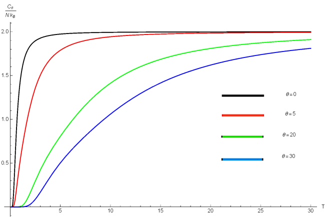
Figure 1: (Color online) The heat capacity versus the temperature $T$ for four values of the noncommutative parameter $\theta=0,5,20,30$.

To accomplish such numerical analysis of the heat capacity $C_{\theta}$, in Figure 2 we plot $C_{\theta}$ in terms of the noncommutative parameter $\theta$ for different values of temperature $T=100K,200K,300K,400K$. It is clearly seen that $C_{\theta}$ decreases rapidly for some values of the temperature but such behavior changes once $T$ increases giving rise different results. Thus, we conclude that the heat capacity can be controlled by changing $\theta$ together with the temperature.

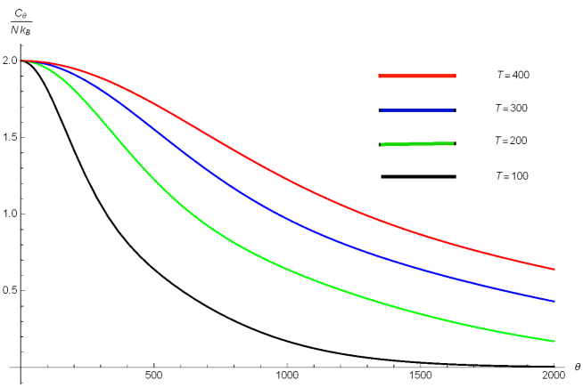
Figure 2: (Color online) The heat capacity versus the noncommutative parameter $\theta$ for four values of the temperature $T=100K,200K,300K,400K$.

4 Effective magnetization

Recall that the present study does not include an external magnetic field but we can still talk about magnetization since $\theta$ is a free parameter. field. Then in analogy, we can define an effective magnetization in the same as for the case of a magnetic field and write

$$M_{\theta}={1\over\beta}{\partial\ln{\mathbb{Z}}_{T}\over\partial\theta}.$$ (27)

After calculation, we end up with

$$M_{\theta}={Nm\omega^{2}\over 2}{\sinh(\beta\varphi_{\theta})-{\theta\over l_{\theta}^{2}}\sinh(\beta\phi_{\theta})\over\cosh(\beta\phi_{\theta})-\cosh(\beta\varphi_{\theta})}$$ (28)

which is depending on $\theta$ as well as the temperature and therefore one can study some limiting cases to underline its behavior. Indeed, at low temperature $(\beta\longrightarrow\infty)$, $M_{\theta}$ becomes

$$M_{\theta}=-\frac{Nm\omega^{2}}{2{\sqrt{1+\left(\frac{2{\hbar}}{m\omega\theta}\right)^{2}}}}$$ (29)

and at high temperature $(\beta\longrightarrow 0)$, we obtain a linear dependence in terms of $\theta$

$$M_{\theta}=-\frac{\beta Nm^{2}\omega^{4}}{24}\theta.$$ (30)

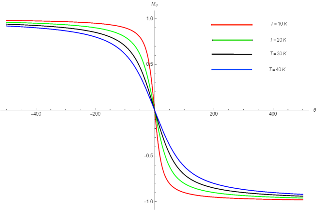
Figure 3: (Color online) The effective magnetization $M_{\theta}$ in terms of the noncommutative parameter $\theta$ for different values of the temperature $T=10K,20K,30K,40K$.

In Figure 3, we plot the effective magnetization versus the noncommutative parameter $\theta$ for different values of the temperature $T$. A very important point is that when the parameter $\theta$ is weak for high or low temperature, $M_{\theta}$ varies in a linear way. However for the case when $\theta$ is strong in low temperature $M_{\theta}$ becomes constant. This tells us that one may use such magnetization to measure the noncommutative parameter.

At this level, we can also introduce the effective susceptibility by adopting that corresponding to the magnetic field and thus have

$$\chi_{\theta}={\partial M_{\theta}\over\partial\theta} = \frac{mN\omega^{2}}{4l_{\theta}^{6}}\ \frac{{2\theta^{2}\sinh\left(\beta\phi_{\theta}\right)}-{2l_{\theta}^{4}\sinh\left(\beta\phi_{\theta}\right)}-{l_{\theta}^{2}\beta\theta^{2}m\omega^{2}\cosh\left(\beta\phi_{\theta}\right)}+l_{\theta}^{6}\beta m\omega^{2}\cosh\left(\beta\varphi_{\theta}\right)}{\cosh\left(\beta\phi_{\theta}\right)-\cosh\left(\beta\varphi_{\theta}\right)}$$ (31)

$$-\frac{\left(l_{\theta}^{2}\sinh\left(\beta\varphi_{\theta}\right)-{\theta\sinh\left(\beta\phi_{\theta}\right)}\right)\left({\beta\theta m\omega^{2}\sinh\left(\beta\phi_{\theta}\right)}-l_{\theta}^{2}\beta m\omega^{2}\sinh\left(\beta\varphi_{\theta}\right)\right)}{2l_{\theta}^{4}\left(\cosh\left(\beta\phi_{\theta}\right)-\cosh\left(\beta\varphi_{\theta}\right)\right){}^{2}}.$$

At high temperature $\beta\longrightarrow 0$, it can be approximated as

$$\chi_{\theta}=-\frac{\beta Nm^{2}\omega^{4}}{12}$$ (32)

which is similar to the well-known Curie law ${C\over T}$ where the Curie constant can be fixed as $C=-{Nm^{2}\omega^{4}\over 12k_{B}}$. It is clearly seen that from (32), the present system behaves like a diamagnetism and also like a superconductor if we require

$$T_{SC}=\frac{12k_{B}}{Nm^{2}\omega^{4}}.$$ (33)

These show that our results are general and can be tuned on to give different interpretations of the present system. On the other hand, one can use them to give a laboratory test of the noncommutative parameter.

5 Bose-Einstein condensation

Let us investigate the relation between the corresponding Bose-Einstein condensation and the noncommutative parameter $\theta$. For this we start by introducing the quantities

$$\omega_{1}={m\omega^{2}l_{\theta}^{2}\over 2}+{m\omega^{2}\theta\over 2},\qquad\omega_{2}={m\omega^{2}l_{\theta}^{2}\over 2}-{m\omega^{2}\theta\over 2},\qquad\varepsilon_{0}={m\omega^{2}l_{\theta}^{2}\over 2}$$ (34)

to rewrite the single-particle energy as

$$E_{n_{g}n_{d}}=\varepsilon+\varepsilon_{0}=\omega_{1}n_{d}+\omega_{2}n_{g}+\varepsilon_{0}.$$ (35)

Unlike the case of fermions, any number of bosons may be placed in a particular micro-state and when the temperature of the system is null, all bosons must be in the ground-state energy $\varepsilon_{0}$. Such number of bosons, that are not in the ground-state $\varepsilon_{0}$, is given by

$$N_{\varepsilon}=\sum_{n_{g},n_{d}=0}^{+\infty}{1\over\exp\left({E_{n_{g}n_{d}}-\mu\over k_{B}T}\right)-1}$$ (36)

where $\mu$ is the chemical potential. Then immediately, we derive the number of bosons in the ground-state $\varepsilon_{0}$

$$N_{\varepsilon=0}=N-N_{\varepsilon>0}.$$ (37)

Note that, when $T$ is high we have $N_{\varepsilon=0}\ll N_{\varepsilon>0}$, but at $T=0$ this is no longer the case because all particles are in the corresponding micro-state $\varepsilon=0$ and therefore we can write

$$\langle N_{\varepsilon=0}\rangle=N={1\over\exp\left({\varepsilon_{0}-\mu\over k_{B}T}\right)-1}.$$ (38)

Now we adopt a procedure similar to that applied in [20, 21] in order to determine the proper density of states $\rho(\varepsilon)$. This latter can be obtained from the number $\nu(\varepsilon)$ of states for which $\varepsilon=\omega_{1}n_{d}+\omega_{2}n_{g}$ is less than or equal to a given energy. To describe the Bose-Einstein condensation we restrict our self to the case where $\theta$ is small and therefore we can make an expansion to write a new frequency $\Omega=\omega_{1}\omega_{2}$ and the ground-state energy as

$$\Omega^{2}=\omega^{2}\left(1-{\theta^{2}\over\alpha^{2}}\right),\qquad\varepsilon_{0}=\hbar\omega\left(1+{\theta^{2}\over 2\alpha^{2}}\right)$$ (39)

which allow to end up with the desired density $\rho(\varepsilon)$

$$\rho(\varepsilon)=\frac{1}{\hbar\omega\sqrt{1-\frac{\theta^{2}}{\alpha^{2}}}}+\frac{\varepsilon}{\left(\hbar\omega\right)^{2}\left(1-\frac{\theta^{2}}{\alpha^{2}}\right)}$$ (40)

where we have defined the parameter $\alpha=\frac{2\hbar}{m\omega}$ that has to fulfill the condition $\alpha>\theta$. To go further, we replace $\omega_{1}n_{d}+\omega_{2}n_{g}$ by a continuous variable $\varepsilon$ and consider (40) to convert the summation over the quantum numbers $n_{d},n_{g}$ on integration over $\varepsilon$. Doing this process to obtain

$$N_{\varepsilon>0}=\int_{0}^{+\infty}{\rho(\varepsilon)\over\exp\left({\varepsilon+\varepsilon_{0}-\mu\over k_{B}T}\right)-1}d\varepsilon$$ (41)

which can be written in terms of the fugacity $z_{\theta}=\exp\left({\mu-\varepsilon_{0}\over k_{B}T}\right)$ as

$$N_{\varepsilon>0}=\frac{1}{\left(\hbar\omega\right)^{2}\left(1-\frac{\theta^{2}}{\alpha^{2}}\right)}\int_{0}^{+\infty}{\varepsilon\over z_{\theta}^{-1}\exp\left({\varepsilon\over k_{B}T}\right)-1}d\varepsilon+\frac{1}{\hbar\omega\sqrt{\left(1-\frac{\theta^{2}}{\alpha^{2}}\right)}}\int_{0}^{+\infty}{1\over z_{\theta}^{-1}\exp\left({\varepsilon\over k_{B}T}\right)-1}d\varepsilon$$ (42)

or equivalently

$$N_{\varepsilon>0}=\frac{\left(k_{B}T\right)^{2}}{\left(\hbar\omega\right)^{2}\left(1-\frac{\theta^{2}}{\alpha^{2}}\right)}\int_{0}^{+\infty}{x\over z_{\theta}^{-1}e^{x}-1}dx+\frac{k_{B}T}{\hbar\omega\sqrt{\left(1-\frac{\theta^{2}}{\alpha^{2}}\right)}}\int_{0}^{+\infty}{1\over z_{\theta}^{-1}e^{x}-1}dx$$ (43)

after making the change of variable $x={\varepsilon\over k_{B}T}$. We show that both of integrals converge only when the fugacity is in the interval $0<z_{\theta}<1$ and therefore we derive a strong condition to obtain the Bose-Einstein condensation that is the noncommutative parameter has to satisfy the following restriction

$$\alpha\sqrt{2\left|\frac{\mu}{\hbar\omega}-1\right|}<\theta<\alpha.$$ (44)

With this, we can now integrate (43) to get

$$N_{\varepsilon>0}=\frac{\left(k_{B}T\right)^{2}}{\left(\hbar\omega\right)^{2}\left(1-\frac{\theta^{2}}{\alpha^{2}}\right)}\text{Li}_{2}\left(z_{\theta}\right)-\frac{k_{B}T}{\hbar\omega\sqrt{\left(1-\frac{\theta^{2}}{\alpha^{2}}\right)}}\ln\left(1-z_{\theta}\right)$$ (45)

where Li is the polylogarithm function. Recall that the Bose temperature $T_{C}$ is that for which $N_{\varepsilon>0}=N$ and then we have

$$T_{C}={\hbar\omega\over k_{B}}\sqrt{\left(1-{\theta^{2}\over\alpha^{2}}\right)}\left(\frac{N}{\text{Li}_{2}\left(z_{\theta}\right)}\right)^{1/2}\left(k_{B}T_{C}\ln\left(1-z_{\theta}\right)\over\hbar\omega\sqrt{\left(1-\frac{\theta^{2}}{\alpha^{2}}\right)}N+1\right)^{1/2}.$$ (46)

Now if the number of particles is very large, then the Bose-Einstein condensation occurs at the temperature

$$T_{0}={\hbar\omega\over k_{B}}\sqrt{\left(1-{\theta^{2}\over\alpha^{2}}\right)}\left(\frac{N}{\text{Li}_{2}\left(z_{\theta}\right)}\right)^{1/2}.$$ (47)

Using (37) and (47) to obtain the ratio

$$\frac{N_{0}}{N}=1-\left(\frac{T}{T_{0}}\right)^{2}+\frac{\ln\left(1-z_{\theta}\right)}{\sqrt{N}\text{Li}_{2}\left(z_{\theta}\right)}\left(\frac{T}{T_{0}}\right).$$ (48)

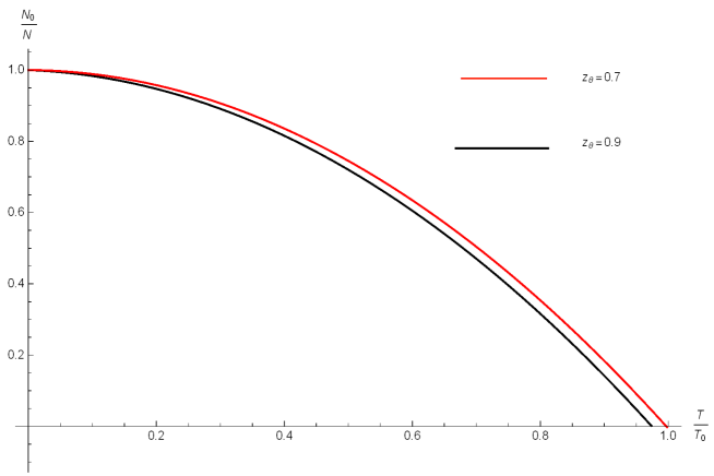
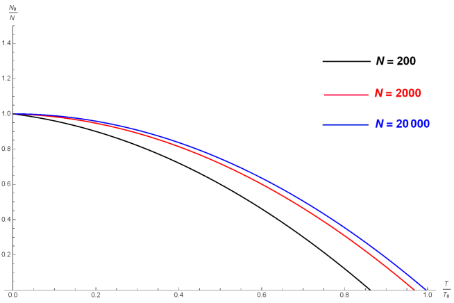
Figure 4: (Color online) The number ratio ${N_{0}\over N}$ versus the temperature ratio ${T\over T_{0}}$ for some values of the fugacity.

In Figure 4 we plot the number ratio ${N_{0}\over N}$ versus the temperature ratio ${T\over T_{0}}$ for some values of the fugacity. The shape of the Bose-Einstein condensation becomes spherical when increasing the fugacity or decreasing the number of particles, which are two parameters governing the ellipticity of the shape of the Bose-Einstein condensation. These are interesting remarks because in the physics we know that the elliptical shape is a consequence of the precise geometry of the trap in which the superfluid is maintained. Thus one can modify such shape by changing the magnetic field that creates this trap. Then in our study we can do the same job by fixing the noncommutative parameter as a magnetic field and then modify the shape of the Bose-Einstein condensation.

Let us look for the relation between the noncommutative parameter and the condensation temperature $T_{C}$ to underline the behavior of the present system. This can be done by considering (45) to show that such relation is given by

$$T_{C}=\frac{\sqrt{4N\text{Li}_{2}\left(z_{\theta}\right)+\log^{2}\left(1-z_{\theta}\right)}+\log\left(1-z_{\theta}\right)}{2\text{Li}_{2}\left(z_{\theta}\right)}.$$ (49)

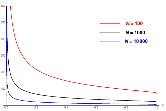
Figure 5: (Color online) The condensation temperature $T_{C}$ versus the fugacity $z_{\theta}$ for some particular values of $N$.

Figure 5 shows that the temperature of condensation is strongly depending on the fugacity, which is a function of the noncommutative parameter $\theta$, together with the number of particles. We observe that when the fugacity is close to zero $T_{c}$ decreases rapidly but when the fugacity increases to move away from zero $T_{c}$ remains almost constant. On the other hand, $T_{c}$ tends to zero when $N$ becomes of the order of $10^{4}$ but if $N$ is of the order of $10^{3}$, $T_{c}$ tends to a non-null value.

6 Conclusion

We have studied the thermodynamic properties and analyzed the Bose-Einstein condensation for a system of $N$ particle living on the noncommutative plane. After building the noncommutative Hamiltonian via star product definition and getting the solution of the energy spectrum, we have determined the partition function $Z_{\theta}$ in terms of the noncommutative parameter $\theta$. This was used to derive the corresponding internal energy and therefore the heat capacity.

Subsequently, we have defined an effective magnetization in similar way to that corresponding to the magnetic field. It was noticed that when the parameter $\theta$ is very low for high or low temperature regimes, the effective magnetization varies in a linear way. On the other hand, by evaluating the associated susceptibility, we have obtained a negative expression at high temperature, which showing similarity with the Curie law for a magnetic system. Finally, we have shown that to get the Bose-Einstein condensation in the present system, one has to fix the noncommutative parameter $\theta$ in a well-defined interval. This was used to establish an interesting relation between the temperature of condensation and $\theta$.

References

- [1] A. Connes, Noncommutative Geometry, (Academic Press 1994).
- [2] R. E. Prange and S. M. Girvin (editors), The Quantum Hall Effect, (SpringerVerlag 1990).
- [3] O. F. Dayi and A. Jellal, J. Math. Phys. 43, 4592 (2002).
- [4] A. Jellal and R. Houça, Int. J. Geom. Meth. Mod. Phys. 6, 343 (2009).
- [5] O. F. Dayi and M. Elbistan, Phys. Lett. A 373, 1314 (2009).
- [6] K. Ma and S. Dulat, Phys. Rev. A 84, 012104 (2011).
- [7] B. Basu, D. Chowdhury and S. Ghosh, Phys. Lett. A 377, 1661 (2013).
- [8] A. Jellal and M. Bellati, Int. J. Geom. Meth. Mod. Phys. 7, 143 (2010).
- [9] J. Gamboa, M. Loewe, F. Mendez and J. C. Rojas, Phys. Rev. D 64, 067901 (2001).
- [10] J. Jing, F. H. Liu and J. F. Chen, Europhys. Lett. 84, 61001 (2008).
- [11] B. Muthukumar and P. Mitra, Phys. Rev. D 66, 027701 (2002).
- [12] J. Jing, S. H. Zhao, J. F. Chen and Z. W. Long, Euro. Phys. J. C 54, 685 (2008).
- [13] A. Das, H. Falomir, M. Nieto, J. Gamboa and F. Mendez, ´ Phys. Rev. D 84, 045002 (2011).
- [14] Wung-Hong Huang and Kuo-Wei Huang, Phys. Lett. B 670, 416 (2009).
- [15] V. Hosseinzadeh, M. A. Gorji, K. Nozari and B. Vakili, Phys. Rev. D 92, 025008 (2015).
- [16] Ahmad Shariati, Mohammad Khorrami and Amir H Fatollahi, J. Phys. A: Math. Theor. 43, 285001 (2010).
- [17] Francisco A. Brito and Elisama E.M. Lima, Int. J. Mod. Phys. A 31, 1650057 (2016).
- [18] S. Bose, Z. Phys. 26, 178 (1924).
- [19] M. H. Anderson, J. R. Ensher, M. R. Mattews, C. E. Wieman and E. A. Corneli, Science 269, 198 (1995).
- [20] S. Grossmann and M. Holthaus, Z. Phys. B 97, 319 (1995).
- [21] S. Grossmann and M. Holthaus, Z. Natureforsch. 50 a, 921-930 (1995).