Jacobi-Galerkin spectral method for eigenvalue problems of Riesz fractional differential equations

Abstract.

An efficient Jacobi-Galerkin spectral method for calculating eigenvalues of Riesz fractional partial differential equations with homogeneous Dirichlet boundary values is proposed in this paper. In order to retain the symmetry and positive definiteness of the discrete linear system, we introduce some properly defined Sobolev spaces and approximate the eigenvalue problem in a standard Galerkin weak formulation instead of the Petrov-Galerkin one as in literature. Poincaré and inverse inequalities are proved for the proposed Galerkin formulation which finally help us establishing a sharp estimate on the algebraic system’s condition number. Rigorous error estimates of the eigenvalues and eigenvectors are then readily obtained by using Babuška and Osborn’s approximation theory on self-adjoint and positive-definite eigenvalue problems. Numerical results are presented to demonstrate the accuracy and efficiency, and to validate the asymptotically exponential oder of convergence. Moreover, the Weyl-type asymptotic law $\lambda_{n}=\mathcal{O}(n^{2\alpha})$ for the $n$-th eigenvalue $\lambda_{n}$ of the Riesz fractional differential operator of order $2\alpha$, and the condition number $N^{4\alpha}$ of its algebraic system with respect to the polynomial degree $N$ are observed.

1. Introduction

Fractional differential equations (FDEs) have been widely used in modeling of many nonlocal phenomena arising from science and engineering, such as viscoelasticity, electromagnetism and so on (see [21, 28, 31, 3, 14, 17] and the references therein), among which the Riesz fractional differential equations are of common interests of mathematicians and physicists. It is widely assumed that Riesz fractional derivatives are equivalent to fractional Laplacians [11]. Riesz FDEs have been numerically studied extensively, including, finite difference method [15], a fourth order compact alternating direction implicit (ADI) scheme [43], finite element methods [9, 42, 18, 32] and spectral methods [39, 26]. In particular, Mao et al. have developed recently a novel spectral Petrov-Galerkin method to solve the boundary value problem of Riesz fractional differential equations and established the error estimate in non-uniformly weighted Sobolev spaces [26].

The eigenvalue problem for the Riesz fractional differential euqations is challenging and has attracted lots of attention (see [22, 8, 30, 38, 40, 37, 34, 16, 29, 23, 44]). Most of the existing studies focus on the theoretical research. Let $\Lambda=(-1,1)$ and $2\alpha\in(0,2)$. Kwaśnicki [22] introduced the Weyl-type asymptotic law for the eigenvalues of the one-dimensional fractional Laplace operator $(-\Delta)^{\alpha}$ on the interval $\Lambda$ with the zero exterior boundary conditions: the $n$-th eigenvalue is equal to $(n\pi/2-(2-2\alpha)\pi/8)^{2\alpha}+\mathcal{O}(1/n)$. DeBlassie [13] and Chen et al. [12] have derived the estimate for $\lambda_{n}$ is $\displaystyle\frac{1}{2}(\frac{n\pi}{2})^{2\alpha}\leq\lambda_{n}\leq(\frac{n\pi}{2})^{2\alpha}$. Meanwhile, owing to the non-locality of Reisz fractional derivatives, it is usually impossible to obtain analytically a closed expression for the eigenfunctions, and it is also hard to precisely specify the (asymptotic) behavior of an eigenfunction $\psi_{k}(x)$ around the endpoints $x=\pm 1$. This motivates researchers to carry out numerical studies on the Riesz differential eigenvalue problem. Zoia et al. [44] have provided a discretized version of the Riesz differential operator of order $2\alpha$. The eigenvalues and eigenfunctions in a bounded domain were then gained numerically for different boundary conditions. However, the eigenfunctions of a Riesz fractional differential operator have only a limited regularity measured in usual Sobolev space, and eigensolutions obtained by ordinary numerical methods have a very poor accuracy. Based on these numerical eigensolutions, analytical results concerning the spectrum structure may not be reliable or even be erroneous in some cases [44]. Indeed, Borthagaray et al. [6] have shown that the first eigenfunction $\psi_{1}$ belongs to $H^{\alpha+1/2-\varepsilon}(\Lambda)$ for any $\varepsilon>0$, and the conforming finite element method exhibits a convergence rate of order $1-\varepsilon$. Hence, one may ask for high order methods to conquer this difficulty.

Fortunately, evidences showed that in general for the eigenfunctions scale as $(1-x^{2})^{\alpha}$ as $x\to\pm 1$ [10, 45] , and the first eigenfunction $\psi_{1}(x)\sim\frac{\Gamma(3/2+2\alpha)}{\sqrt{\pi}\Gamma(1+2\alpha)}(1-x^{2})^{\alpha}$ as $2\alpha\to+\infty$ [7]. Using the Jacobi basis functions $\{(1-x^{2})^{\alpha}J^{\alpha,\alpha}_{n}(x)\}_{n=0}^{N}$ to mimic the singular behavior of the eigenfunctions, one may naturally expect a spectrally high order of convergence rate of the specifically devised spectral method for the eigenvalue problems.

The main purpose of this paper is thus to propose an efficient Jacobi-Galerkin spectral method for solving Riesz fractional differential eigenvalue problems, and then to conduct a comprehensive numerical analysis.

We start with a brief review over some definitions of Riesz fractional derivatives on the interval $\Lambda$. Some Sobolev spaces are then introduced to fit the domain of Riesz fractional derivatives, in which the Riesz fractional derivatives are proved to be self-adjoint and positive definite. Thus, the Riesz fractional differential eigenvalue problems can be equivalently written in a symmetric weak formulation. This recognition eventually helps us to propose a Jacobi-Galerkin spectral method, instead of the Petrov-Galerkin one, for solving Riesz fractional differential eigenvalue problems. Moreover, by adopting the generalized Jacobi functions as the basis functions, an efficient implementation is given for this Jacobi-Galerkin spectral method. Indeed, the stiffness matrix is identity owing to orthonormality of the basis function with respect to the inner product induced by Riesz fractional operators; while all entries of the mass matrix can be explicitly evaluated via their analytical formula.

The symmetric variational formulation also play an important role in the numerical analysis. On the one hand, the Poincaré inequality and the inverse inequality for Riesz fractional derivatives are derived, through which the lower and the upper bounds of all eigenvalues are established, respectively. Moreover, an elaborative analysis shows that the smallest numerical eigenvalue behaves as $\mathcal{O}(1)$ while the largest one of the Riesz fractional differential operator of order $2\alpha$ behaves as $\mathcal{O}(N^{4\alpha})$. This indicates that the condition number of the mass matrix increases at a rate of $\mathcal{O}(N^{4\alpha})$. On the other hand, following the approximation theory of Babuška and Osborn on the Ritz method for self-adjoint and positive-definite eigenvalue problems, rigorous error estimates for both the eigenvalues and eigenfunctions are presented.

Numerical experiments demonstrate that our Jacobi-Galerkin method has a higher accuracy than all existing methods ever known. Indeed, asymptotically exponential (sub-geometric) orders of convergence are observed for large $N$ in the error plots in both semi-logarithm and logarithm-logarithm scales. This hypothesis is also convinced by a reliability analysis of all computational eigenvalues together with a continuity analysis of the first eigenvalue upon the fractional order $2\alpha$. Besides, the order of $\mathcal{O}(N^{4\alpha})$ for the condition number of the reduced linear algebraic eigen-system (also of the mass matrix) is also confirmed numerically.

The remainder of this paper is organized as follows. We describe some notations and preliminary results about the fractional derivatives operators in Section 2. In Section 3, we propose an efficient Jacobi-Galerkin spectral method for the Riesz fractional differential eigenvalue problem with homogeneous Dirichlet boundary conditions. The detail of the numerical implementation is also described. Furthermore, the rigorous error estimate of the valid eigenvalues and eigenvectors is derived by the approximation theory of Babuška and Osborn on the Ritz method for self-adjoint and positive-definite eigenvalue problems. Some numerical results which verify the efficiency and accuracy of the Jacobi-Galerkin spectral method are provided in Section 4. Finally, a conclusion remark is made in the last section.

2. Preliminaries

Throughout this paper, we shall use the notations $a\lesssim b$ for $a\leq Cb$, $a\gtrsim b$ for $a\geq cb$, and $a\asymp b$ for $cb\leq a\leq Cb$ with some generic positive constants $c$ and $C$ which are independent of any function and of any discretization parameters. Next denote by $\mathbb{N}$ (resp. $\mathbb{R}$) the set of positive integers (resp. real numbers). Further denote $\mathbb{N}_{0}:=\{0\}\cup\mathbb{N}$.

Let $\omega$ be a generic positive weight function which is not necessary in $L^{1}(I)$ ($I\subseteq\mathbb{R}$). Denote by $(u,v)_{\omega,I}:=\int_{I}u(x)\overline{v(x)}\omega(x)dx$ the inner product of $L^{2}_{\omega}(I)$ with the norm $\|\cdot\|_{\omega,I}$. Whenever $I=\Lambda:=(-1,1)$, the subscript $I$ will be omitted.

2.1. Fractional integrals and derivatives

Furthermore, we recall the definitions of the fractional integrals and derivatives in the sense of Riemann-Liouville.

$\mathbf{Definition~{}1}$ (Fractional integrals and derivatives). For $\rho>0$, the left and right fractional integral are defined respectively as

$${}_{-1}I^{\rho}_{x}v(x): =\displaystyle\frac{1}{\Gamma(\rho)}\int\limits_{-1}^{x}\frac{v(t)}{(x-t)^{1-\rho}}dt,\quad x>-1,$$

$${}_{x}I^{\rho}_{1}v(x): =\displaystyle\frac{1}{\Gamma(\rho)}\int\limits^{1}_{x}\frac{v(t)}{(t-x)^{1-\rho}}dt,\quad x<1.$$

For real $s\in[k-1,k)$ with $k\in\mathbb{N}$, the left-side and the right-side Riemann-Liouville fractional derivative (LRLFD and RRLFD) of order $s$ are defined respectively by

$${}_{-1}D^{s}_{x}v(x): =\displaystyle\frac{1}{\Gamma(k-s)}\frac{d^{k}}{dx^{k}}\int\limits_{-1}^{x}\frac{v(t)}{(x-t)^{s-k+1}}dt,x\in\Lambda,$$

$${}_{x}D^{s}_{1}v(x): =\displaystyle\frac{(-1)^{k}}{\Gamma(k-s)}\frac{d^{k}}{dx^{k}}\int\limits^{1}_{x}\frac{v(t)}{(t-x)^{s-k+1}}dt,x\in\Lambda.$$

$\mathbf{Definition~{}2}$ (Fractional Riesz integral and derivatives). For $\rho>0$, the Riesz fractional integrals are defined as

$$I_{1}^{\rho}v(x): =\displaystyle\frac{1}{2\Gamma(\rho)\sin\frac{\pi\rho}{2}}\int\limits_{-1}^{1}\frac{\mbox{sgn}(x-t)}{|x-t|^{1-\rho}}v(t)dt=\frac{1}{2\sin\frac{\pi\rho}{2}}({}_{-1}I^{\rho}_{x}-{}_{x}I^{\rho}_{1})v(x), x\in\Lambda,\,\frac{\rho}{2}\not\in\mathbb{N},$$

$$I_{2}^{\rho}v(x): =\displaystyle\frac{1}{2\Gamma(\rho)\cos\frac{\pi\rho}{2}}\int\limits_{-1}^{1}\frac{v(t)}{|x-t|^{1-\rho}}dt=\frac{1}{2\cos\frac{\pi\rho}{2}}({}_{-1}I^{\rho}_{x}+{}_{x}I^{\rho}_{1})v(x), x\in\Lambda,\,\frac{\rho+1}{2}\not\in\mathbb{N},$$

where sgn is the sign function.

For $s\in[k-1,k)$ with $k\in\mathbb{N}$, we define the Riesz fractional derivative (RFD) of order $s$:

(1) $$D^{s}v(x):=\frac{(-1)^{\lfloor\frac{s+1}{2}\rfloor}}{2\cos\frac{\pi s}{2}}\big{[}{}_{-1}D_{x}^{s}+{}_{x}D_{1}^{s}\big{]}v(x)=\begin{cases}\dfrac{d^{k}}{dx^{k}}I_{1}^{k-s}v(x),&k\text{ odd},\\[5.0pt] \dfrac{d^{k}}{dx^{k}}I_{2}^{k-s}v(x),&k\text{ even},\end{cases}\qquad x\in\Lambda,$$

hereafter $\lfloor a\rfloor$ is the greatest integer not exceeding the real number $a$. Whenever $s$ is an odd integer, the definition of $D^{s}v$ is then treated in the limit sense.

Let us define the Fourier transform of a function $u\in L^{2}(\mathbb{R})$,

$$\widehat{v}(\xi)=[\mathscr{F}v](\xi)=\int_{\mathbb{R}}v(x)\operatorname{e}^{-\operatorname{i}\xi x}dx,\quad\xi\in\mathbb{R}.$$

Further let $\tilde{v}$ be the zero extension of $v$,

(2) $$\tilde{v}\big{|}_{\Lambda}=v\quad\text{ and }\quad\tilde{v}\big{|}_{\mathbb{R}\setminus\Lambda}=0.$$

Then one finds the following alternative definition of the Riesz fractional integral and derivative [33],

$$[\mathscr{F}(I_{1}^{\rho}v)](\xi)=-\operatorname{i}\mathrm{sgn}(\xi)\,|\xi|^{-\rho}\,[\mathscr{F}\tilde{v}](\xi),\qquad\qquad[\mathscr{F}(I_{2}^{\rho}v)](\xi)=|\xi|^{-\rho}\,[\mathscr{F}\tilde{v}](\xi),$$

(3) $$[\mathscr{F}(D^{s}v)](\xi)=(-1)^{\lfloor\frac{s+1}{2}\rfloor}|\xi|^{s}[\mathscr{F}\tilde{v}](\xi)=\begin{cases}(-1)^{\frac{k}{2}}|\xi|^{s}[\mathscr{F}\tilde{v}](\xi),&k\text{ even},\\ (-1)^{\frac{k-1}{2}}|\xi|^{s}[\mathscr{F}\tilde{v}](\xi),&k\text{ odd},\end{cases}\qquad v\in\mathscr{D}(\Lambda),$$

which implies that, for any $n\in\mathbb{N}_{0}$, $D^{2n}=(-1)^{n}\dfrac{d^{2n}}{dx^{2n}}$, while $D^{2n+1}$ is totally distinct from $\dfrac{d^{2n+1}}{dx^{2n+1}}$.

Remark 1.

We would like to emphasize the equivalence of Riesz fractional derivative and the fractional Laplacian. Indeed, among several ways to define the fractional Laplacian $(-\Delta)^{s/2}$ on the (bounded) interval $\Lambda$, the one using the zero extension and the pseudo-differential operator of symbol $|\xi|^{s}$ is of our greatest interest [1],

(4) $$(-\Delta)^{s/2}v(x)=[\mathscr{F}^{-1}(|\xi|^{s}\mathscr{F}\tilde{v})](x),$$

which reveals that the Riesz fractional derivative (1) on $\Lambda$ coincides, up to a constant $\pm 1$, with the fractional Laplacian (4).

2.2. Sobolev spaces

It is well known that $H^{s}(\mathbb{R})$ can be defined through the Fourier transform [25, 36, 20],

(5) $$\begin{split}&H^{s}(\mathbb{R})=\big{\{}v\in\mathscr{D}^{\prime}(\mathbb{R}):\|v\|_{s,\mathbb{R}}<\infty\big{\}},\\ &|v|_{s,\mathbb{R}}=\Big{(}\frac{1}{2\pi}\int_{\mathbb{R}}\ {|\xi|}^{2s}\big{|}\widehat{v}({\xi})\big{|}^{2}d{\xi}\Big{)}^{\frac{1}{2}},\qquad\qquad\|v\|_{s,\mathbb{R}}=\Big{(}\frac{1}{2\pi}\int_{\mathbb{R}}\big{(}1+|\xi|^{2}\big{)}^{s}\big{|}\widehat{v}({\xi})\big{|}^{2}d{\xi}\Big{)}^{\frac{1}{2}};\end{split}$$

and $H^{s}(\Lambda)$ ($s\geq 0$) can be derived from $H^{s}(\mathbb{R})$ by extension [20, 25, 36],

(6) $$H^{s}(\Lambda)=\big{\{}v=u|_{\Lambda}:u\in H^{s}(\mathbb{R})\big{\}}, \|v\|_{s}=\inf_{u\in H^{s}(\mathbb{R})\atop u|_{\Lambda}=v}\|u\|_{s,\mathbb{R}}.$$

The completion of $\mathscr{D}(\Lambda)$ in $H^{s}(\Lambda)$ is denoted by $H^{s}_{0}(\Lambda)$.

The zero extension $\tilde{v}$ of $v$ as defined in (2) is of particular interest [20, 25]. By Theorem 11.4 of [25], $v\mapsto\tilde{v}$ is a continuous mapping of $H^{s}(\Lambda)\mapsto H^{s}(\mathbb{R})$ if and only if $0\leq s<\frac{1}{2}$, is a continuous mapping of $H_{0}^{s}(\Lambda)\mapsto H^{s}(\mathbb{R})$ for $s>\frac{1}{2}$ if and only if $s+\frac{1}{2}\not\in\mathbb{N}$.

The zero extension induces a special type of Sobolev spaces,

$$H^{s}_{*}(\Lambda)=\left\{v\in\mathscr{D}^{\prime}(\Lambda):\tilde{v}\in H^{s}(\mathbb{R})\right\},\qquad\|v\|_{s,*}=\|\tilde{v}\|_{s,\mathbb{R}},\ |v|_{s,*}=|\tilde{v}|_{s,\mathbb{R}}.$$

Actually, $\mathscr{D}(\Lambda)$ is dense in $H^{s}_{*}(\Lambda)$ for $s\geq 0$ [36, Theorem 3.2.4/1], thus the completion of $\mathscr{D}(\Lambda)$ in $H^{s}_{*}(\Lambda)$ is $H^{s}_{*}(\Lambda)$ itself, i.e., space $H^{s}_{*0}(\Lambda)=H^{s}_{*}(\Lambda)$. More precisely, it holds that

$$H^{s}_{*0}(\Lambda)=H^{s}_{*}(\Lambda)=\begin{cases}H^{s}(\Lambda)=H^{s}_{0}(\Lambda),&\text{ if }0<s<\frac{1}{2},\\ H^{s}_{00}(\Lambda)\subset H^{s}_{0}(\Lambda),&\text{ if }s+\frac{1}{2}\in\mathbb{N},\\ H^{s}_{0}(\Lambda)\subset H^{s}(\Lambda),&\text{ if }s>\frac{1}{2},\ s+\frac{1}{2}\not\in\mathbb{N},\end{cases}$$

where the interpolation space $H^{m+\frac{1}{2}}_{00}(\Lambda)=[H^{m}_{0}(\Lambda),H^{m+1}_{0}(\Lambda)]_{\frac{1}{2}}$.

Indeed, according to [25], $(-1)^{m}D^{2m}$ ($m\in\mathbb{N}$) is self-adjoint, positive and unbounded in $H_{0}^{2m}(\Lambda)$, which is dense in $H^{0}(\Lambda)=L^{2}(\Lambda)$ with continuous injection. Moreover, $\|v\|_{2m}^{2}\asymp\|v\|^{2}+\|D^{2m}v\|^{2}\asymp\|D^{2m}v\|^{2}\asymp|v|_{2m}^{2}$ for all $v\in H^{2m}_{0}(\Lambda)$. Thus by the space interpolation theory,

(7) $$H^{s}_{*}(\Lambda)=[H^{0}(\Lambda),H^{2m}_{0}(\Lambda)]_{\frac{s}{2m}}=\left\{v\in\mathscr{D}^{\prime}(\Lambda):\|v\|^{2}+\|D^{s}v\|^{2}<\infty\right\}.$$

For any $s\in[k-\frac{1}{2},k+\frac{1}{2})$ with the positive integer $k$, one readily obtains from the adjoint properties of the Riemann-Liouville fractional differential operators that [19, 24, 27]

(8) $$(-1)^{k}(D^{2s}u,v)=(D^{s}u,D^{s}v)=(-1)^{k}(u,D^{2s}v),\qquad u,v\in H_{*}^{s}(\Lambda).$$

Moreoever, by (3) together with Parserval’s theorem,

(9) $$|v|_{s,*}=\|D^{s}v\|:=|v|_{s}.$$

Indeed, by Lemma 1.3.2.6 in [20], it holds for $0\leq s<1$ that

(10) $$\|v\|_{s,*}^{2}\asymp|v|_{s,*}^{2}\asymp|v|_{s}^{2}+\|v\|_{\omega^{-2s,-2s}}^{2},\qquad v\in H_{*}^{s}(\Lambda),$$

where $\omega^{\alpha,\alpha}=\omega^{\alpha,\alpha}(x)=(1-x^{2})^{\alpha}$.

We now conclude this subsection with the following embedding theorem.

Theorem 1.

$H^{s}_{*}(\Lambda)$ with $s>0$ is compactly embedded in $L^{2}(\Lambda)$, i.e., $H^{s}_{*}(\Lambda)\hookrightarrow L^{2}(\Lambda)$.

Proof.

One first notes that $H^{s}(\Lambda)$ ($s>0$) is compactly embedded in $L^{2}(\Lambda)$ and $H^{s}_{*}(\Lambda)\subseteq H^{s}(\Lambda)$, then Theorem 1 is readily checked. ∎

2.3. Generalized Jacobi functions

Let $P_{n}^{\alpha,\beta}(x),\,n\in\mathbb{N}_{0}$ with $\alpha,\beta>-1$ be the classical Jacobi polynomials which are orthogonal with respect to the weight function $\omega^{\alpha,\beta}(x)=(1-x)^{\alpha}(1+x)^{\beta}$ over $\Lambda$, i.e.

(11) $$(P_{n}^{\alpha,\beta},P_{m}^{\alpha,\beta})_{\omega^{\alpha,\beta}}=\gamma_{n}^{\alpha,\beta}\delta_{nm},\qquad\gamma_{n}^{\alpha,\beta}=\frac{2^{\alpha+\beta+1}}{2n+\alpha+\beta+1}\,\frac{\Gamma(n+\alpha+1)\Gamma(n+\beta+1)}{n!\Gamma(n+\alpha+\beta+1)},$$

where $\delta_{nm}$ is the Dirac delta symbol.

We now define a special type of generalized Jacobi functions:

(12) $$\mathcal{J}_{n}^{-\alpha,-\alpha}(x)=(1-x^{2})^{\alpha}P_{n}^{\alpha,\alpha}(x),\qquad x\in\Lambda,\,n\in\mathbb{N}_{0},\,\alpha>-1.$$

It is clear that $\mathcal{J}_{n}^{-\alpha,-\alpha}(x),n\in\mathbb{N}_{0}$, satisfy the homogeneous boundary conditions

(13) $$\partial_{x}^{l}\mathcal{J}_{n}^{-\alpha,-\alpha}(\pm 1)=0,\quad l=0,1,\cdots,\lceil\alpha\rceil-1,$$

where $\lceil\alpha\rceil$ stands for the smallest integer not less than $\alpha.$

Lemma 1.

If $\alpha>0$, $2\alpha\in[2k-1,2k+1)$ and $\nu\in\{0,1,\dots,\lfloor\alpha\rfloor\}$, then

(14) $$D^{2\alpha-2\nu}\mathcal{J}_{n}^{-\alpha,-\alpha}(x)=(-1)^{k}\dfrac{2^{2\nu}\Gamma(n+2\alpha-2\nu+1)}{n!}P^{\alpha-2\nu,\alpha-2\nu}_{n+2\nu}(x),\quad n\in\mathbb{N}_{0}.$$

Proof.

We resort to the following identities on the Riesz integral of Jacobi functions [31, Theorem 6.5 and Theorem 6.7],

(15) $$\begin{split}\int_{-1}^{1}\frac{\omega^{\frac{s-1}{2}+i,\frac{s-1}{2}+j}(t)P^{\frac{s-1}{2}+i,\frac{s-1}{2}+j}_{n}(t)}{|x-t|^{s}}dt=\frac{\pi(-1)^{i}2^{i+j}\Gamma(n+s)}{n!\Gamma(s)\cos\frac{s\pi}{2}}P^{\frac{s-1}{2}-i,\frac{s-1}{2}-j}_{n+i+j}(x),\\ x\in(-1,1),\ s\in(0,1),\ i,j\in\mathbb{Z},\ i,j>-\frac{s+1}{2},\ n+i+j\geq 0;\end{split}$$

(16) $$\begin{split}\int_{-1}^{1}\frac{\mathrm{sgn}(x-t)}{|x-t|^{s}}\omega^{\frac{s}{2}+i,\frac{s}{2}+j}(t)P^{\frac{s}{2}+i,\frac{s}{2}+j}_{n}(t)dt=\frac{\pi(-1)^{i}2^{i+j+1}\Gamma(n+s)}{n!\Gamma(s)\sin\frac{s\pi}{2}}P^{\frac{s}{2}-i-1,\frac{s}{2}-j-1}_{n+i+j+1}(x),\\ x\in(-1,1),\ s\in(0,1),\ i,j\in\mathbb{Z},\ i,j>-\frac{s+2}{2},\ n+i+j+1\geq 0.\end{split}$$

Thus, by taking $s=2\alpha-2k$ and $i=j=k$ when $2\alpha\in[2k,2k+1)$, we derive that

$$I_{1}^{2k+1-2\alpha}\mathcal{J}^{-\alpha,-\alpha}_{n}(x)=\frac{(-1)^{k}2^{2k+1}\Gamma(n+2\alpha-2k)}{n!}P^{\alpha-2k-1,\alpha-2k-1}_{n+2k+1}(x),$$

$$D^{2\alpha-2\nu}\mathcal{J}^{-\alpha,-\alpha}_{n}(x)=\frac{(-1)^{k}2^{2k+1}\Gamma(n+2\alpha-2k)}{n!}\frac{d^{2k+1-2\nu}}{dx^{2k+1-2\nu}}P^{\alpha-2k-1,\alpha-2k-1}_{n+2k+1}(x)$$

$$\qquad=\frac{(-1)^{k}2^{2\nu}\Gamma(n+2\alpha-2\nu+1)}{n!}P^{\alpha-2\nu,\alpha-2\nu}_{n+2\nu}(x);$$

While, by taking $s=2\alpha-2k+1$ and $i=j=k$ when $2\alpha\in[2k-1,2k)$, we also get that

$$I_{2}^{2k-2\alpha}\mathcal{J}^{-\alpha,-\alpha}_{n}(x)=\frac{(-1)^{k}2^{2k}\Gamma(n+2\alpha-2k+1)}{n!}P^{\alpha-2k,\alpha-2k}_{n+2k}(x),$$

$$D^{2\alpha-2\nu}\mathcal{J}^{-\alpha,-\alpha}_{n}(x)=\frac{(-1)^{k}2^{2k}\Gamma(n+2\alpha-2k+1)}{n!}\frac{d^{2k-2\nu}}{dx^{2k-2\nu}}P^{\alpha-2k,\alpha-2k}_{n+2k}(x)$$

$$\qquad=\frac{(-1)^{k}2^{2\nu}\Gamma(n+2\alpha-2\nu+1)}{n!}P^{\alpha-2\nu,\alpha-2\nu}_{n+2\nu}(x).$$

The proof is now completed. ∎

By (8), (14) and (11), one arrives at the following theorem.

Theorem 2.

$\mathcal{J}_{m}^{-\alpha,-\alpha},\ m\geq 0$ form a complete orthogonal system in $H_{*}^{\alpha}(\Lambda)$. More precisely,

(17) $$(D^{\alpha}\mathcal{J}_{m}^{-\alpha,-\alpha},D^{\alpha}\mathcal{J}_{n}^{-\alpha,-\alpha})=\frac{2^{2\alpha+1}\Gamma(m+\alpha+1)^{2}}{m!^{2}(2m+2\alpha+1)}\delta_{m,n},\qquad m,n\in\mathbb{N}_{0},\,\alpha\geq 0.$$

As an immediate consequence of Theorem 2, any $u\in H_{*}^{s}(\Lambda)$ has an expansion in generalized Jacobi functions,

(18) $$u(x)=\sum_{i=0}^{\infty}u_{i}\mathcal{J}^{-s,-s}_{i}(x),\qquad u_{i}=\frac{(D^{s}u,D^{s}\mathcal{J}^{-s,-s}_{i})}{(D^{s}\mathcal{J}^{-s,-s}_{i},D^{s}\mathcal{J}^{-s,-s}_{i})},$$

and

(19) $$|u|_{s}^{2}=\sum_{i=0}^{\infty}\frac{2^{2\alpha+1}\Gamma(i+\alpha+1)^{2}}{i!^{2}(2i+2\alpha+1)}|u_{i}|^{2}.$$

3. Riesz fractional differential eigenvalue problems and Jacobi-Galerkin approximation

3.1. Riesz fractional differential eigenvalue problems

We consider the Riesz fractional differential eigenvalue problems of order $2\alpha\in[2k-1,2k+1)$ with $k\in\mathbb{N}$,

(20) $$\begin{cases}(-1)^{k}D^{2\alpha}u(x)=\lambda u(x),&x\in\Lambda,\\ u^{(l)}(\pm 1)=0,&l=0,1,\cdots,k-1.\end{cases}$$

The weak formulation of (20) reads: to find nontrivial $(\lambda,u)\in\mathbb{R}\times H^{\alpha}_{*}(\Lambda)$, such that

(21) $$a(u,v)=\lambda b(u,v),\qquad v\in H^{\alpha}_{*}(\Lambda),$$

where $a(\cdot,\cdot)$ and $b(\cdot,\cdot)$ are the bilinear forms defined by

$$a(u,v) =(D^{\alpha}u,D^{\alpha}v),\quad u,v\in H^{\alpha}_{*}(\Lambda),$$

$$b(u,v) =(u,v), u,v\in L^{2}(\Lambda).$$

It is obvious that $a(\cdot,\cdot)$ and $b(\cdot,\cdot)$ are symmetric, positive definite, continuous and coercive on $H^{\alpha}_{*}(\Lambda)\times H^{\alpha}_{*}(\Lambda)$ and $L^{2}(\Lambda)\times L^{2}(\Lambda)$, respectively.

Remark 2.

We would like to point out that unlike the weak formulation in [26], our weak formulation (21) here is formulated in a standard symmetrical way, which is convenient for us to conduct the numerical analysis on eigenvalue problems of the fractional differential equations.

Remark 3.

Problem (20) admits an infinite sequence of eigensolutions $\{(\lambda_{i},\psi_{i})\}_{i=1}^{\infty}$ with the eigenvalues being ordered increasingly, $\lambda_{1}<\lambda_{2}\leq\lambda_{3}\leq\cdots$. All eigenvalues of (20) are real and positive. Moreover, it is proved that all eigenvalues are simple if $\frac{1}{2}<\alpha\leq 2$ [22]. Besides the following proposition on the Poincaré inequality indicates,

$$\lambda_{1}>\Gamma(2\alpha+1).$$

Proposition 1.

(Poincaré inequality) Suppose $u\in H^{\alpha}_{*}(\Lambda)\setminus\{0\}$, then

(22) $$|u|_{\alpha,*}>\sqrt{\Gamma(2\alpha+1)}\,\|u\|_{\omega^{-\alpha,-\alpha}}>\sqrt{\Gamma(2\alpha+1)}\,\|u\|.$$

Proof.

For any $i\in\mathbb{N}_{0}$,

$$\frac{\Gamma(i+2\alpha+1)}{i!}=\frac{(i+2\alpha)(i+2\alpha-1)\cdots(2\alpha+1)}{i!}\,\Gamma(2\alpha+1)>\Gamma(2\alpha+1).$$

Then, for any $u\in H^{\alpha}_{*}(\Lambda)$ with $u(x)=\displaystyle\sum_{i=0}^{\infty}u_{i}\mathcal{J}_{i}^{-\alpha,-\alpha}(x),$ we get from (17), (11) together with the Parseval’s identities that

$$|u|_{\alpha}^{2}= \,\sum_{i=0}^{\infty}\frac{\Gamma(i+2\alpha+1)}{i!}\frac{2^{2\alpha+1}\Gamma(i+\alpha+1)^{2}}{i!\Gamma(i+2\alpha+1)(2i+2\alpha+1)}|u_{i}|^{2}$$

$$> \,\Gamma(2\alpha+1)\sum_{i=0}^{\infty}\frac{2^{2\alpha+1}\Gamma(i+\alpha+1)^{2}}{i!\Gamma(i+2\alpha+1)(2i+2\alpha+1)}|u_{i}|^{2}$$

$$= \,\Gamma(2\alpha+1)\|u\|_{\omega^{-\alpha,-\alpha}}^{2}>\Gamma(2\alpha+1)\|u\|^{2},$$

which completes the proof. ∎

3.2. Jacobi-Galerkin spectral approximation and implementation

Let $\mathbb{P}_{N}$ be the set of polynomials with degree less than or equal to $N$. Then, we define the finite dimensional fractional space for $\alpha>0$,

$$\mathbb{F}_{N}^{-\alpha,-\alpha}(\Lambda):=\mbox{span}\Big{\{}\phi_{n}(x):=\frac{\sqrt{2n+2\alpha+1}\,n!}{2^{\alpha+\frac{1}{2}}\,\Gamma(n+\alpha+1)}\mathcal{J}_{n}^{-\alpha,-\alpha}(x),0\leq n\leq N\Big{\}}.$$

The Jacobi-Galerkin spectral method for (21) can be written as follows, to find $(\lambda_{N},u_{N})\in\mathbb{R}\times\mathbb{F}_{N}^{-\alpha,-\alpha}(\Lambda)$ such that

(23) $$a(u_{N},v_{N})=\lambda_{N}b(u_{N},v_{N}),\qquad v_{N}\in\mathbb{F}_{N}^{-\alpha,-\alpha}(\Lambda).$$

We now give a brief description on the numerical implementation of the Jacobi Galerkin spectral method for the Riesz fractional differential eigenvalue problems. Firstly, we expand $u_{N}(x)$ with the unknowns $\{u_{j}\}^{N}_{j=0}$ as follows,

(24) $$u_{N}(x)=\sum^{N}_{j=0}u_{j}\phi_{j}(x).$$

By inserting the expansions of (24) into (23) and taking the test functions $v_{N}=\phi_{i}(x),\,i=0,1,\dots,N$, then problem (23) can be written in the following matrix form:

(25) $$S\overline{u}=\lambda_{N}B\overline{u},$$

where the coefficient vector $\overline{u}=(u_{0},u_{1},\dots,u_{N})^{\mathsf{T}}$, and the stiffness and mass matrices $S=(S_{ij})_{0\leq i,j\leq N}$ and $M=(M_{ij})_{0\leq i,j\leq N}$ are determinated by the following lemma.

Lemma 2.

It holds that

(26) $$S_{ij}=(D^{\alpha}\phi_{j},D^{\alpha}\phi_{i})=\delta_{ij},$$

(27) $$M_{ij}=(\phi_{j},\phi_{i})=\begin{cases}\frac{(-1)^{\frac{j-i}{2}}\sqrt{\pi(2i+2\alpha+1)(2j+2\alpha+1)}\,\Gamma(2\alpha+1)(i+j)!}{2^{2\alpha+i+j+1}\,\Gamma(2\alpha+\frac{i+j}{2}+\frac{3}{2})\,\Gamma(\alpha+\frac{i-j}{2}+1)\,\Gamma(\alpha+\frac{j-i}{2}+1)\left(\frac{i+j}{2}\right)!},&i+j\text{ even},\\ 0,&i+j\text{ odd}.\end{cases}$$

Proof.

Owing to the orthogonality relation (17), one readily verifies (26).

By a parity argument, one also finds that $M_{ij}=0$ whenever $i+j$ is odd. To prove (27) for even $i+j$, we shall resort to the following connection identity of two Jacobi polynomials [2, Theorem 7.1.4],

(28) $$\begin{split}P^{\gamma,\gamma}_{n}(x)=&\,\sum_{\nu=0}^{\lfloor\frac{n}{2}\rfloor}c^{\gamma,\alpha}_{n,\nu}P^{\alpha,\alpha}_{n-2\nu}(x),\\ c^{\gamma,\alpha}_{n,\nu}:=&\,\frac{(\gamma+1)_{n}(2\alpha+1)_{n-2\nu}(\gamma+\frac{1}{2})_{n-\nu}(\alpha+\frac{3}{2})_{n-2\nu}(\gamma-\alpha)_{\nu}}{(2\gamma+1)_{n}(\alpha+1)_{n-2\nu}(\alpha+\frac{3}{2})_{n-\nu}(\alpha+\frac{1}{2})_{n-2\nu}\nu!},\end{split}$$

where the Pochhammer symbol $(a)_{\nu}=\frac{\Gamma(a+\nu)}{\Gamma(a)}$.

Indeed, by Rodrigues’ formula and integration by parts, one obtains

$$\,\int_{-1}^{1}(1-x^{2})^{\alpha}P^{\alpha,\alpha}_{j}(x)(1-x^{2})^{\alpha}P^{\alpha,\alpha}_{i}(x)dx=\frac{(-1)^{j+i}}{2^{j+i}j!i!}\int_{-1}^{1}\partial_{x}^{j}(1-x^{2})^{j+\alpha}\cdot\partial_{x}^{i}(1-x^{2})^{i+\alpha}dx$$

$$= \,\frac{(-1)^{j}}{2^{j+i}j!i!}\int_{-1}^{1}(1-x^{2})^{i+\alpha}\partial_{x}^{j+i}(1-x^{2})^{j+\alpha}dx=\frac{(-1)^{i}(j+i)!}{j!i!}\int_{-1}^{1}(1-x^{2})^{2\alpha}P_{j+i}^{\alpha-i,\alpha-i}(x)dx,$$

where the $P_{j+i}^{\alpha-i,\alpha-i}$ is a generalized Jacobi polynomial as discussed in [35, §4.22] whenever $\alpha-i\leq-1$. To proceed, we utilize (28) to expand $P^{\alpha-i,\alpha-i}_{j+i}$ as $\sum_{\nu=0}^{\lfloor\frac{i+j}{2}\rfloor}c^{\alpha-i,2\alpha}_{i+j,\nu}P^{2\alpha,2\alpha}_{i+j-2\nu}$. Due the orthogonality (11) of Jacobi polynomials, we derive that

$$\int_{-1}^{1}(1-x^{2})^{\alpha}P^{\alpha,\alpha}_{j}(x)(1-x^{2})^{\alpha}P^{\alpha,\alpha}_{i}(x)dx=\frac{(-1)^{i}(j+i)!}{j!i!}\int_{-1}^{1}(1-x^{2})^{2\alpha}c^{\alpha-i,2\alpha}_{j+i,\frac{j+i}{2}}P_{0}^{2\alpha,2\alpha}(x)dx$$

$$= \,\frac{(-1)^{i}(j+i)!}{j!i!}\frac{(\alpha-i+1)_{j+i}(\alpha-i+\frac{1}{2})_{\frac{j+i}{2}}(-i-\alpha)_{\frac{j+i}{2}}}{(2\alpha-2i+1)_{j+i}(2\alpha+\frac{3}{2})_{\frac{j+i}{2}}\frac{j+i}{2}!}\gamma^{2\alpha,2\alpha}_{0}$$

$$= \,\frac{(-1)^{\frac{j-i}{2}}(j+i)!}{2^{j+i}j!i!}\frac{(-j-\alpha)_{\frac{j+i}{2}}(-i-\alpha)_{\frac{j+i}{2}}}{(2\alpha+\frac{3}{2})_{\frac{j+i}{2}}\frac{j+i}{2}!}\frac{\sqrt{\pi}\,\Gamma(2\alpha+1)}{\Gamma(2\alpha+\frac{3}{2})}.$$

Finally, (27) with even $i+j$ is an immediate consequence of the above equation. This ends the proof. ∎

It is worthy to point out that the algebraic eigenvalue problem (25) can be decoupled into two according to even or odd modes.

3.3. Numerical analysis

In this subsection, we first give some estimates on the magnitudes of the smallest and greatest numerical eigenvalues, and thus on the condition number of the mass matrix $M$. Then the error estimates for both the eigenvalues and eigenfunctions are presented.

Let $\{(\lambda_{i,N},\psi_{i,N})\}_{i=1}^{N+1}$ be the eigensolutions of (23) such that $\lambda_{1,N}\leq\lambda_{2,N}\leq\cdots\leq\lambda_{N+1,N}$. The following Lemma indicates each the numerical eigenvalue satisfies $\lambda_{i,N}\lesssim N^{4\alpha}$.

Lemma 3.

(Inverse inequality) Suppose $u_{N}\in\mathbb{F}_{N}^{-\alpha,-\alpha}(\Lambda)$, then

(29) $$\|D^{\alpha}u_{N}\|^{2}\lesssim N^{4\alpha}\,\|u_{N}\|^{2}.$$

Proof.

For any $u_{N}(x)=\displaystyle\sum_{i=0}^{N}u_{i}\mathcal{J}_{i}^{-\alpha,-\alpha}(x)\in\mathbb{F}_{N}^{-\alpha,-\alpha}(\Lambda),$ we have

(30) $$\|D^{\alpha}u\|^{2}= \displaystyle\sum_{i=0}^{N}\frac{\Gamma(i+2\alpha+1)}{i!}u_{i}^{2}\gamma_{i}^{\alpha,\alpha}\lesssim N^{2\alpha}\displaystyle\sum_{i=0}^{N}u_{i}^{2}\gamma^{\alpha,\alpha}_{n},$$

where we have used the following estimate [26, (3.26)] for the inequality sign above,

$$\frac{\Gamma(i+2\alpha+1)}{i!}\lesssim i^{2\alpha}\lesssim N^{2\alpha},\qquad 0\leq i\leq N.$$

Meanwhile, we note that [5, Corollary 6.2 of page 99],

$$\|\psi_{N}\|_{\omega^{\alpha,\alpha}}\lesssim N^{\alpha}\|\psi_{N}\|_{\omega^{2\alpha,2\alpha}},\qquad\forall\psi_{N}(x)\in\mathbb{P}_{N}(\Lambda).$$

Since $\omega^{-\alpha,-\alpha}u_{N}\in\mathbb{P}_{N}(\Lambda)$, we now derive that

(31) $$\|u_{N}\|^{2}= \big{\|}\omega^{-\alpha,-\alpha}u_{N}\big{\|}_{\omega^{2\alpha,2\alpha}}^{2}\gtrsim N^{-2\alpha}\big{\|}\omega^{-\alpha,-\alpha}u_{N}\big{\|}_{\omega^{\alpha,\alpha}}^{2}=N^{-2\alpha}\sum_{i=0}^{N}u_{i}^{2}\gamma_{i}^{\alpha,\alpha}.$$

A combination of (30) and (31) then yields (29). This completes the proof. ∎

The following theorem gives some sharp estimates on the numerical eigenvalues.

Theorem 3.

Its holds that

(32) $$\lambda_{1,N}=\mathcal{O}(1),\quad\lambda_{N+1,N}=\mathcal{O}(N^{4\alpha}),$$

as $N$ tends to infinity. Further, the spectral condition number of the mass matrix $M$ satisfies

(33) $$\chi_{N}(M)=\frac{\lambda_{N+1,N}}{\lambda_{1,N}}=\mathcal{O}(N^{4\alpha}).$$

Proof.

Since (33) is an immediate consequence of (32), we only need to prove (32).

Thanks to the Min-Max principle and Lemma 2,

$$\lambda_{1}= \min_{u\in H^{s}_{*}(I)}\frac{\|D^{\alpha}u\|^{2}}{\|u\|^{2}}\leq\min_{u\in\mathbb{F}^{-\alpha,-\alpha}_{N}(\Lambda)}\frac{\|D^{\alpha}u\|^{2}}{\|u\|^{2}}=\lambda_{1,N},$$

$$\lambda_{1,N}= \,\min_{u\in\mathbb{F}^{-\alpha,-\alpha}_{N}(\Lambda)}\frac{\|D^{\alpha}u\|^{2}}{\|u\|^{2}}\leq\frac{\|D^{\alpha}\phi_{0}\|^{2}}{\|\phi_{0}\|^{2}}=\frac{1}{M_{00}}$$

$$= \,\frac{2^{2\alpha+1}\Gamma(2\alpha+\frac{3}{2})\Gamma(\alpha+1)^{2}}{\sqrt{\pi}\,\Gamma(2\alpha+2)}=\frac{\Gamma(2\alpha+\frac{3}{2})\Gamma(\alpha+1)}{\Gamma(2\alpha+2)\Gamma(\alpha+\frac{3}{2})},$$

where $M_{00}$ which yields that $\lambda_{1,N}=\mathcal{O}(1)$.

Next, by the inverse equality (29), we find that

$$\lambda_{N+1,N}=\max_{\mathbb{F}^{-\alpha,-\alpha}_{N}(\Lambda)}\frac{\|D^{\alpha}u\|^{2}}{\|u\|^{2}}\lesssim N^{4\alpha}.$$

To prove $\lambda_{N+1,N}=\mathcal{O}(N^{4\alpha})$, it then suffices to verify that

(34) $$\|D^{\alpha}\eta_{N}\|^{2}=\mathcal{O}(N^{8\alpha+2}),\quad\|\eta_{N}\|^{2}=\mathcal{O}(N^{4\alpha+2}), N\to+\infty.$$

where

$$\eta_{N}(x)=\frac{\Gamma(N+4\alpha+3)}{\Gamma(N+2\alpha+2)}(1-x^{2})^{\alpha}P^{2\alpha+1,2\alpha+1}_{N}(x)\in\mathbb{F}^{-\alpha,-\alpha}_{N}(\Lambda).$$

Indeed, by (28),

$$\eta_{N}(x) =(1-x^{2})^{\alpha}\sum_{\nu=0}^{\lfloor N/2\rfloor}\frac{4\,\Gamma(N-2\nu+4\alpha+1)\,(N-2\nu+2\alpha+1/2)}{\Gamma(N-2\nu+2\alpha+1)}P^{2\alpha,2\alpha}_{N-2\nu}(x).$$

Then the orthogonality (11) reveals that

$$\|\eta_{N}\|^{2} =\sum_{\nu=0}^{\lfloor N/2\rfloor}\frac{16\,\Gamma(N-2\nu+4\alpha+1)^{2}\,(N-2\nu+2\alpha+1/2)^{2}\times 2^{4\alpha+1}\,\Gamma(N-2\nu+2\alpha+1)^{2}}{\Gamma(N-2\nu+2\alpha+1)^{2}\times(2N-4\nu+4\alpha+1)\,(N-2\nu)!\,\Gamma(N-2\nu+4\alpha+1)}$$

$$=2^{4\alpha+4}\sum_{\nu=0}^{\lfloor N/2\rfloor}\frac{\Gamma(N-2\nu+4\alpha+1)(N-2\nu+2\alpha+1/2)}{(N-2\nu)!}$$

$$=\mathcal{O}(N^{4\alpha+2}),$$

where the last equality sign is derived by using the fact that [33, (1.66)]

$$\lim_{z\to+\infty}\frac{\Gamma(z+\alpha)}{\Gamma(z)z^{\alpha}}=1,\qquad\alpha>0.$$

Meanwhile, the connection relation (28) gives

$$\eta_{N}(x) =(1-x^{2})^{\alpha}\frac{\Gamma(4\alpha+3)\Gamma(\alpha+1/2)}{\Gamma(2\alpha+2)\Gamma(2\alpha+1)\Gamma(2\alpha+3/2)}$$

$$\times\sum_{\nu=0}^{\lfloor N/2\rfloor}\frac{(N-2\nu+\alpha+1/2)\Gamma(N-2\nu+2\alpha+1)\Gamma(N-\nu+2\alpha+3/2)\Gamma(\nu+\alpha+1)}{\Gamma(N-2\nu+\alpha+1)\Gamma(N-\nu+\alpha+3/2)\nu!}P^{\alpha,\alpha}_{N-2\nu}(x),$$

which together with the orthogonality (17) impiles

$$\|D^{\alpha}\eta_{N}\|^{2} =\frac{2^{2\alpha}\Gamma(4\alpha+3)^{2}\Gamma(\alpha+1/2)^{2}}{\Gamma(2\alpha+2)^{2}\Gamma(2\alpha+1)^{2}\Gamma(2\alpha+3/2)^{2}}$$

$$\times\sum_{\nu=0}^{\lfloor N/2\rfloor}\frac{(N-2\nu+\alpha+1/2)\,\Gamma(N-2\nu+2\alpha+1)^{2}\,\Gamma(N-\nu+2\alpha+3/2)^{2}\,\Gamma(\nu+\alpha+1)^{2}}{(N-2\nu)!^{2}\,\Gamma(N-\nu+\alpha+3/2)^{2}\,\nu!^{2}}$$

$$=\mathcal{O}(N^{8\alpha+2}).$$

This gives (34) and the proof is now completed. ∎

We now concentrate on the error estimates for the numerical eigenvalues and eigenfunctions. Let us define the orthogonal projector $\Pi_{N}^{-\alpha,-\alpha}:H^{\alpha}_{*}(\Lambda)\rightarrow\mathbb{F}_{N}^{-\alpha,-\alpha}(\Lambda)$, such that for all $u\in H^{\alpha}_{*}(\Lambda)$,

$$\begin{array}[]{l}(D^{\alpha}(\Pi_{N}^{-\alpha,-\alpha}u-u),D^{\alpha}v_{N})=0,\qquad v_{N}\in\mathbb{F}_{N}^{-\alpha,-\alpha}(\Lambda).\end{array}$$

Then we introduce the Sobolev space for any $\alpha>0$, $\nu\in\{0,1,\dots,\lfloor\alpha\rfloor\}$, $m\in\mathbb{N}_{0},m\geq 2\nu-\lfloor\alpha\rfloor$,

$$\mathcal{B}_{\alpha,\nu}^{m}(\Lambda)=\{v\in L^{2}_{\omega^{-\alpha,-\alpha}}(\Lambda):\frac{d^{l}}{dx^{l}}D^{2\alpha-2\nu}v\in L^{2}_{\omega^{\alpha-2\nu+l,\alpha-2\nu+l}},\ 0\leq l\leq m\}.$$

Lemma 4.

Assume $\alpha>0$, $\nu\in\{0,1,\dots,\lfloor\alpha\rfloor\}$. Then for all $u\in\mathcal{B}_{\alpha,\nu}^{m}(\Lambda)$ with $m\geq 2\nu-\lfloor\alpha\rfloor$, we have the following estimate,

(35) $$\|D^{\alpha}(\Pi_{N}^{-\alpha,-\alpha}u-u)\|\lesssim N^{2\nu-\alpha-m}\Big{\|}\frac{d^{m}}{dx^{m}}D^{2\alpha-2\nu}u\Big{\|}_{\omega^{\alpha-2\nu+m,\alpha-2\nu+m}}.$$

Proof.

By (14), one has

$$\frac{d^{m}}{dx^{m}} D^{2\alpha-2\nu}\mathcal{J}^{-\alpha,-\alpha}_{i}(x)=(-1)^{\lfloor\alpha+\frac{1}{2}\rfloor}\frac{\Gamma(i+2\alpha-2\nu+1)}{2^{-2\nu}i!}\frac{d^{m}}{dx^{m}}P^{\alpha-2\nu,\alpha-2\nu}_{i+2\nu}(x)$$

$$=(-1)^{\lfloor\alpha+\frac{1}{2}\rfloor}\frac{\Gamma(i+2\alpha-2\nu+m+1)}{2^{m-2\nu}i!}P^{\alpha-2\nu+m,\alpha-2\nu+m}_{i+2\nu-m}(x).$$

Further by the orthogonality of the Jacobi polynomials (11), one obtains

$$\Big{(}\frac{d^{m}}{dx^{m}} D^{2\alpha-2\nu}\mathcal{J}^{-\alpha,-\alpha}_{i},\frac{d^{m}}{dx^{m}}D^{2\alpha-2\nu}\mathcal{J}^{-\alpha,-\alpha}_{n}\Big{)}_{\omega^{\alpha-2\nu+m,\alpha-2\nu+m}}$$

$$=\frac{2^{2\alpha+1}\Gamma(i+\alpha+1)^{2}}{(2i+2\alpha+1)i!^{2}}\frac{\Gamma(i+2\alpha-2\nu+m+1)}{\Gamma(i+2\nu-m+1)}\delta_{in}.$$

Thus for any $u=\sum_{i=0}^{\infty}u_{i}\mathcal{J}^{-\alpha,-\alpha}_{i}\in\mathcal{B}^{m}_{\alpha,\nu}(\Lambda)\subseteq H_{*}^{\alpha}(I)$,

$$\Big{\|}\frac{d^{m}}{dx^{m}}D^{2\alpha-2\nu}u\Big{\|}^{2}_{\omega^{\alpha-2\nu+m,\alpha-2\nu+m}}=\sum_{i=0}^{\infty}\frac{2^{2\alpha+1}\Gamma(i+\alpha+1)^{2}}{(2i+2\alpha+1)i!^{2}}\frac{\Gamma(i+2\alpha-2\nu+m+1)}{\Gamma(i+2\nu-m+1)}|u_{i}|^{2}.$$

Meanwhile, by the definition of $\Pi_{N}^{-\alpha,-\alpha}$, it can be readily checked that

$$\Pi_{N}^{-\alpha,-\alpha}u=\sum_{i=0}^{N}u_{i}\mathcal{J}^{-\alpha,-\alpha}_{i}.$$

Then one gets from (17) that

$$\|D^{\alpha}( \Pi_{N}^{-\alpha,-\alpha}u-u)\|^{2}=\sum_{i=N+1}^{\infty}\frac{2^{2\alpha+1}\Gamma(i+\alpha+1)^{2}}{(2i+2\alpha+1)i!^{2}}|u_{i}|^{2}$$

$$=\frac{\Gamma(N+2\nu-m+1)}{\Gamma(N+2\alpha-2\nu+m+1)}$$

$$\quad\times\sum_{i=N+1}^{\infty}\frac{(N+2\nu-m+1)_{i-N}}{\Gamma(N+2\alpha-2\nu+m+1)_{i-N}}\frac{2^{2\alpha+1}\Gamma(i+\alpha+1)^{2}}{(2i+2\alpha+1)i!^{2}}\frac{\Gamma(i+2\alpha-2\nu+m+1)}{\Gamma(i+2\nu-m+1)}|u_{i}|^{2}$$

$$\leq\frac{\Gamma(N+2\nu-m+2)}{\Gamma(N+2\alpha-2\nu+m+2)}\sum_{i=0}^{\infty}\frac{2^{2\alpha+1}\Gamma(i+\alpha+1)^{2}}{(2i+2\alpha+1)i!^{2}}\frac{\Gamma(i+2\alpha-2\nu+m+1)}{\Gamma(i+2\nu-m+1)}|u_{i}|^{2}$$

$$\lesssim N^{4\nu-2m-2\alpha}\Big{\|}\frac{d^{m}}{dx^{m}}D^{2\alpha-2\nu}u\Big{\|}^{2}_{\omega^{\alpha-2\nu+m,\alpha-2\nu+m}},$$

where the following estimate has been used for the first inequality sign,

$$\frac{(N+2\nu-m+1)_{i-N}}{\Gamma(N+2\alpha-2\nu+m+1)_{i-N}}\leq 1,\qquad\alpha+m-2\nu\geq 0.$$

This finally completes the proof. ∎

Recall that $a(\cdot,\cdot)$ is symmetric, continuous and coercive on $H^{\alpha}_{*}(\Lambda)\times H^{\alpha}_{*}(\Lambda)$, $b(\cdot,\cdot)$ is continuous on $L^{2}(\Lambda)\times L^{2}(\Lambda)$, and $H^{\alpha}_{*}(\Lambda)$ is compactly imbedded in $L^{2}(\Lambda)$. Thus, by the approximation theory of Babuška and Osborn on the Ritz method for self-adjoint and positive-definite eigenvalue problems [4, pp. 697-700], we now arrive at the following main theorem.

Theorem 4.

Let $\lambda_{j}$ be an eigenvalue of (20) with the geometric multiplicity $q$ and assume that $\lambda_{j}=\lambda_{j+1}=\dots=\lambda_{j+q-1}$. Denote

$$E(\lambda_{j}):=\left\{\psi\text{ is an eigenfunction corresponding to }\lambda_{j}\text{ with }\|D^{\alpha}\psi\|=1\right\}.$$

Further suppose $\psi\in\mathcal{B}_{\alpha,\nu}^{m}(\Lambda)$ with $\nu\in\{0,1,\dots,\lfloor\alpha\rfloor\}$ and $m\geq 2\nu-\alpha$ for any $\psi\in E(\lambda_{j})$. It holds that

$$0\leq\lambda_{i,N}-\lambda_{j}\lesssim N^{4\nu-2\alpha-2m}\sup_{\psi\in E(\lambda_{j})}\Big{\|}\frac{d^{m}}{dx^{m}}D^{2\alpha-2\nu}\psi\Big{\|}_{\omega^{\alpha-2\nu+m,\alpha-2\nu+m}}^{2},\quad i=j,j+1,\dots,j+q-1.$$

Let $\psi_{i,N}$ be an eigenfunction corresponding to $\lambda_{i,N}$ such that $\|D^{\alpha}\psi_{i,N}\|=1$. Then for $i=j,j+1,\dots,j+q-1$, there holds that

$$\inf_{u\in E(\lambda_{j})}\|u-\psi_{i,N}\|_{\alpha,*}\lesssim N^{2\nu-\alpha-m}\sup_{\psi\in E(\lambda_{j})}\Big{\|}\frac{d^{m}}{dx^{m}}D^{2\alpha-2\nu}\psi\Big{\|}_{\omega^{\alpha-2\nu+m,\alpha-2\nu+m}}.$$

Moreover, for $\psi\in E(\lambda_{j})$, there exists a function $v_{N}\in\mathrm{span}\{\psi_{j,N},\dots,\psi_{j+q-1,N}\}$ such that

$$\|\psi-v_{N}\|_{\alpha,*}\lesssim N^{2\nu-\alpha-m}\sup_{\psi\in E(\lambda_{j})}\Big{\|}\frac{d^{m}}{dx^{m}}D^{2\alpha-2\nu}\psi\Big{\|}_{\omega^{\alpha-2\nu+m,\alpha-2\nu+m}}.$$

4. Numerical results

In this section, we will give some numerical results to illustrate the accuracy and efficiency of the Jacobi-Galerkin spectral method for the Riesz fractional differential eigenvalue problems on the reference domain and validate other theoretical results related.

Example 1.

Fractional derivative order $2\alpha\in(0,2]$.

We begin with $2\alpha\in(0,2]$. This example includes three parts. The first test is to verify the spectral accuracy, while another two tests are to confirm the Weyl-type asymptotic law and the asymptotic behavior of the linear algebraic system’s condition number respectively.

4.1. Accuracy and convergence test – algebraic order or exponential order?

The five leading eigenvalues obtained by our Jacobi-Galerkin spectral method with $N=64$, are listed in Table 1 for different $2\alpha$. They are at least 10 digits accurate, with significant places being estimated from the results with $N=48$. This demonstrates the accuracy of our proposed method. In Table 2, we report the first three eigenvalues by Jacobi-Galerkin spectral method with $N=64$ for other various $2\alpha$ and the numerical approximations to $\lambda_{n}$ provided by the low order method in Ref. [44] with the total degrees of freedom $5000$. We can observe that they are in good agreement.

Table 1. The 5 leading eigenvalues for each $2\alpha$, computed with $N=64$, listed with significant places estimated from the $N=48$ results.

$2\alpha=1.2$	$2\alpha=1.4$	$2\alpha=1.6$	$2\alpha=1.8$	$2\alpha=2.0$
1.29699577674	1.48323343195	1.7282959570964	2.048734983129	2.467401100272
3.4867305364	4.45817398389	5.75634828003	7.50311692608	9.86960440108
5.911679975	8.1507167266	11.31189330097	15.799894163321	22.2066099024
8.534441423	12.424353637	18.1773428791	26.724243284906	39.47841760435
11.29243001	17.162347657	26.1872040516	40.11423380506	61.68502750680

Table 2. Comparison of the first three eigenvalues by Jacobi-Galerkin spectral method with $N=64$ and numerical approximations to $\lambda_{n}$ obtained by the method of Ref.[44] with $5000\times 5000$ matrices.

	$\lambda_{1}$		$\lambda_{2}$		$\lambda_{3}$
$2\alpha$	Present	Ref.[44]	Present	Ref.[44]	Present	Ref.[44]
0.01	0.9966	0.997	1.0087	1.009	1.0137	1.014
0.1	0.9725	0.973	1.0921	1.092	1.1473	1.148
0.2	0.9574	0.957	1.1965	1.197	1.3190	1.320
0.5	0.9701	0.970	1.6015	1.601	2.0288	2.031
1.0	1.1577	1.158	2.7547	2.754	4.3168	4.320
1.5	1.5975	1.597	5.0597	5.059	9.5943	9.957
1.8	2.0487	2.048	7.5031	7.501	15.7998	15.801
1.9	2.2440	2.243	8.5957	8.593	18.7168	18.718
1.99	2.4436	2.2442	9.7331	9.729	21.8286	21.829

To investigate the convergence order of our method, we utilize MAPLE with a precision of 30 digits to establish an even more accurate computational environment. Taking the eigenvalues computed with $N=200$ as the reference eigenvalues, the errors of the first eigenvalue versus polynomial degree $N$ have been plotted in Figs. 1 and 2 with various $2\alpha$ in logarithm-logarithm scale (left) and semi-logarithm (center). The down-bending curves in the logarithm-logarithm plots indicate that the errors decay faster than algebraically as $N$ increases, and asymptotically exponential orders of convergence for fractional differential order $2\alpha$ can be observed in the semi-logarithm plot for large $N.$ Indeed, the log-log plot of $\log(\lambda_{1,N}-\lambda_{1})$ (right) reveals that our Jacobi-Galerkin spectral method converges at a sub-geometric rate $\mathcal{O}(\exp(-qN^{r}))$ with $0<r<1$ for a given $\alpha\not\in\mathbb{N}_{0}$.

Clearly, the first eigenvalue grows exponentially as $2\alpha$ increases as displayed in the left side of Fig. 3, and it converges algebraically to the first Laplacian eigenvalue as $2\alpha$ approaches $2$ (see the right side of Fig. 3). These also confirm the asymptotically exponential order of convergence of our method. By the way, the dashed line for the Gamma function $\Gamma(2\alpha+1)$ in the left side of Fig. 3 shows the lower bound of the numerical eigenvalues, which is in agreement to with the Poincaré inequality in Proposition 1.

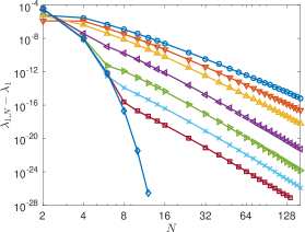
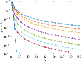
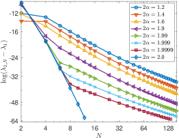
Figure 1. Errors of the first eigenvalue versus polynomial degree $N$ with various fractional orders. Left: $\lambda_{1,N}-\lambda_{1}$ in logarithm-logarithm scale; Center: $\lambda_{1,N}-\lambda_{1}$ in semi-logarithm scale; Right: $\log(\lambda_{1,N}-\lambda_{1})$ in logarithm-logarithm scale.

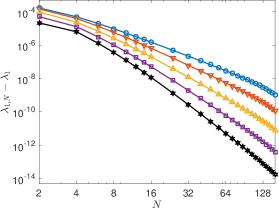
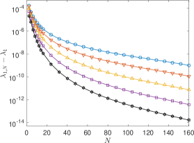
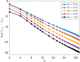
Figure 2. Errors of the first eigenvalue versus polynomial degree $N$ with various fractional orders. Left: $\lambda_{1,N}-\lambda_{1}$ in logarithm-logarithm scale; Center: $\lambda_{1,N}-\lambda_{1}$ in semi-logarithm scale; Right: $\log(\lambda_{1,N}-\lambda_{1})$ in logarithm-logarithm scale.

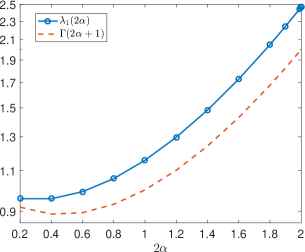
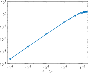
Figure 3. Left: The first eigenvalue and the reference function $\Gamma(2\alpha+1)$ for different fractional partial order $2\alpha$ from $0.2$ to $2.0$ in semi-logarithm scale. Right: $\lambda_{1}(2)-\lambda_{1}(2\alpha)$ versus $2-2\alpha$ in logarithm-logarithm scale.

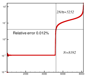
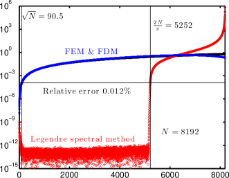
Figure 4. Reliable eigenvalues and their relative errors. Left: $2\alpha=1.6$; Right: $2\alpha=2$.

We plot in Fig. 4 (left) the relative errors for $8192$ numerical eigenvalues for $2\alpha=1.6$ by applying the Jacobi-Galerkin spectral method with the polynomial degree $N=8192$, where the errors have been evaluated by comparing these numerical eigenvalues with the reference solution by $N=10240$. The error curve of the spectral method cuts the intersection of the horizonal line $y=0.012\%$ and the vertical line $x=2N/\pi$. This observation confirms that there are about $2N/\pi$ numerical eigenvalues are reliable, for which the relative error converges at a rate of at least $\mathcal{O}(N^{-1})$. To make a comparison with the Legendre spectral method for Laplacian eigenvalues, we excerpt a similar plot from [41] on the right side, which is actually provided by the third author of this paper. It indicates that the Jacobi-Galerkin spectral method for Riesz fractional eigenvalues behaves asymptotically as the same as the Legendre spectral for Laplacian eigenvalues, which strongly supports our hypothesis on the asymptotically exponential order of convergence.

Finally, we plot in Fig. 5 the first three eigenvectors with different fractional order $2\alpha=1.2,1.6,2.0$ and $N=32$. Here the eigenvectors are all normalized by $L^{2}$-norm.

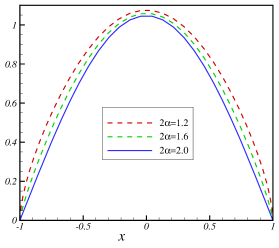
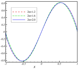
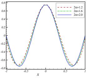
Figure 5. The figure of the first three eigenvectors with different fractional order $2\alpha=1.2,1.6,2.0$ and $N=32$.

4.2. Weyl-type asymptotic law

By a fixed computational parameter $N=1024$, we plot all the eigenvalues with $N=1024$ for different fractional order $2\alpha=1.2,1.4,1.6,1.8,2.0$ in Fig. 6 (left). As expected, it is about $\displaystyle\frac{2}{\pi}\approx 64\%$ of total eigenvalues that are reliable and obey the Weyl-type asymptotic law. Then, the first 700 eigenvalues and function $n^{2\alpha}$ correspond to $2\alpha=1.2$ and $2.0$ are plotted in Fig. 7, which clearly shows the eigenvalues linear dependence of $n^{2\alpha}$.

Fig. 6 (right) presents the 100-th, 200-th, 300-th, 400-th, 500-th, 600-th eigenvalues versus $2\alpha=1.1$ to $2.0$ in semi-logarithm scale. The straight lines indicate that the valid eigenvalues increase algebraic with respect to the fractional order parameter $2\alpha$.

Finally, we plot in Fig. 8 the first 650 values $\rho_{n}=\displaystyle\frac{\lambda_{n}}{(\frac{\pi n}{2})^{2\alpha}}$ versus the $n$ for some $2\alpha$. As we known, the exact eigenvalue $\lambda_{n}$ of $2\alpha=2$ is equal to $\displaystyle(\frac{\pi n}{2})^{2}$, so the corresponding $\rho_{n}$ is identical to $1$ which was checked in Fig. 8. Also, we can conclude that $\lambda_{n}=\displaystyle(\frac{\pi n}{2})^{2\alpha}$ when $n$ is large enough by this figure. In order to better observe the growth tendency of some leading eigenvalues, we plot the $\rho_{n}$ in the sub-figure of Fig. 8 in logarithm-logarithm scale. It shows that the $\rho_{n}$ slightly increases to 1 as $n$ increases for each $2\alpha$.

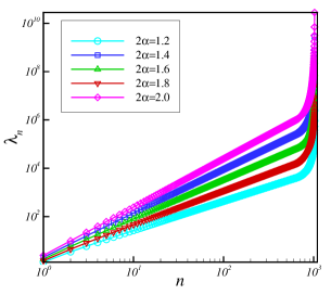
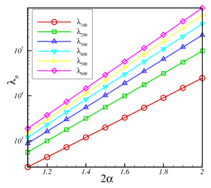
Figure 6. Left: The all eigenvalues with different fractional order $2\alpha$ from $1.2$ to $2.0$, $N=1024$. Right: The $n$-th eigenvalue versus different fractional order $2\alpha$ from $1.1$ to $2.0$ in semi-logarithm scale.

(a) $2\alpha=1.2$

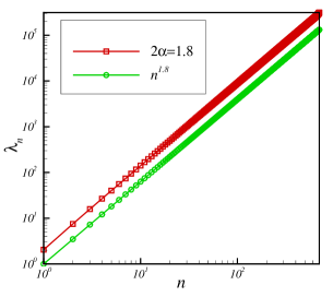
(b) $2\alpha=1.8$

Figure 7. The first 700 eigenvalues and function $n^{2\alpha}$ versus $2\alpha=1.2$ and $2.0$, with $N=1024$.

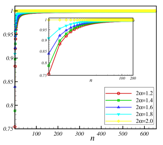
Figure 8. The first 650 values $\rho_{n}=\displaystyle\frac{\lambda_{n}}{(\frac{\pi n}{2})^{2\alpha}}$ versus $n$ for different fractional partial order $2\alpha$ from $1.2$ to $2.0$. The sub-figure plots the first 200 values of $\rho_{n}$ versus $n$ in logarithm-logarithm scale.

4.3. Condition number

In this subsection, we plot in Fig. 9 the condition number versus polynomial degree $N$ with different fractional order $2\alpha$ from $1.2$ to $2.0$ in logarithm-logarithm scale. The result presented in Fig. 9 shows that, for each $2\alpha$, the condition number $\chi_{N}$ grows algebraically with respect to $N$. In order to investigate the growth tendency of the condition number numerically, we plot the condition number together with the function $N^{4\alpha}$ in logarithm-logarithm scale with fixed $2\alpha=1.2$ and $1.8$ in the left and right of Fig. 10 respectively. The straight lines are evidence of $\chi_{N}=\mathcal{O}(N^{4\alpha})$ which was predicted by Theorem 3.

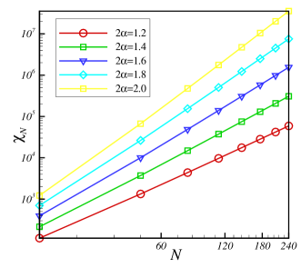
Figure 9. The condition number versus the polynomial degree $N$ with different fractional order $2\alpha$ from $1.2$ to $2.0$ in logarithm-logarithm scale.

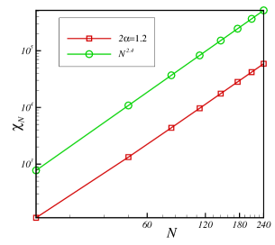
(a) $2\alpha=1.2$

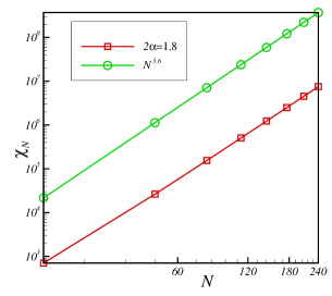
(b) $2\alpha=1.8$

Figure 10. The condition number and polynomial function $N^{4\alpha}$ versus the polynomial degree $N$ with different fractional order $2\alpha=1.2$ and $2\alpha=1.8$ in logarithm-logarithm scale.

Example 2.

Higher fractional derivative order $2\alpha$

In this example, we repeat the tests of the eigenvalue problems with more higher fractional derivative order $2\alpha$. We plot the accuracy, eigenvalues and condition number for $2\alpha=3.6$ and $5.6$ in Figs. 11, 12 (left), 12 (right) and 13 respectively. This numerical results demonstrate that the Jacobi-Galerkin spectral method is still accurate and efficient with larger $2\alpha$.

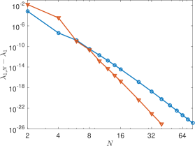
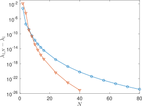
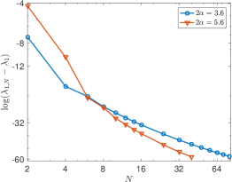
Figure 11. Errors of the first eigenvalue versus polynomial degree $N$ with various fractional orders. Left: $\lambda_{1,N}-\lambda_{1}$ in logarithm-logarithm scale; Center: $\lambda_{1,N}-\lambda_{1}$ in semi-logarithm scale; Right: $\log(\lambda_{1,N}-\lambda_{1})$ in logarithm-logarithm scale.

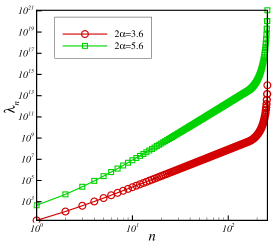
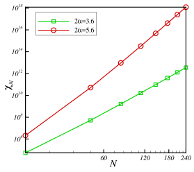
Figure 12. Left: The all eigenvalues with different fractional order $2\alpha$ equal to $3.6$ and $5.6$, $N=256$. Right: The condition number versus the polynomial degree $N$ with different fractional order $2\alpha=3.6$ and $2\alpha=5.6$ in logarithm-logarithm scale.

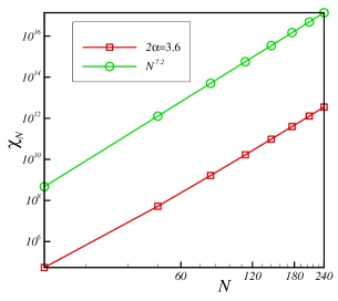
(a) $2\alpha=3.6$

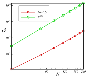
(b) $2\alpha=5.6$

Figure 13. The condition number and polynomial function $N^{4\alpha}$ versus the polynomial degree $N$ with different fractional order $2\alpha=3.6$ and $2\alpha=5.6$ in logarithm-logarithm scale.

5. Conclusion

In this paper, we have proposed an efficient Jacobi-Galerkin spectral method for the Riesz fractional differential eigenvalue problems. The error estimate for the eigenvalues was derived by the compact spectral theory. Numerical results confirm the asymptotically exponential convergence rate of the eigenvalues. Also the eigenvalues with different fractional partial differential order were calculated. The figures demonstrate that the eigenvalues behavior as $n^{2\alpha}$ which obey the Weyl-type asymptotic law. In the future, we will consider the fractional differential eigenvalue problems in two dimensional case and more complex computational domain.

References

• [1] Gabriel Acosta and Juan Pablo Borthagaray. A fractional Laplace equation: regularity of solutions and finite element approximation. SIAM J. Numer. Anal., 55(2):472–495, 2017.
• [2] G. E. Andrews, R. Askey, and R. Roy. Special Functions. Cambridge University Press, 1999.
• [3] A. Babakhani and V. Daftardar-Gejji. Existence of positive solutions of nonlinear fractional differential equations. J. Math. Anal. Appl., 278(2):434–442, 2003.
• [4] I. Babuška and J. Osborn. Eigenvalue problems. Numerical Analysis, 2:641–787, 1991.
• [5] C. Bernardi, M. Dauge, and Y. Maday. Polynomials in the Sobolev World. Numerical Analysis, 2007.
• [6] Juan Pablo Borthagaray, Leandro M. Del Pezzo, and Sandra Martinez. Finite element approximation for the fractional eigenvalue problem. arXiv:0706.1254, 2016.
• [7] Albrecht. Böttcher and Harold Widom. From Toeplitz eigenvalues through Green’s kernels to higher-order Wirtinger-Sobolev inequalities. Operator Theory: Advances and Applications, 171:73 C87, 2006.
• [8] L. Brasco and E. Parini. The second eigenvalue of the fractional $p-$Laplacian. Adv. Calc. Var., 2015.
• [9] W.P. Bu, Y.F. Tang, and J.Y. Yang. Galerkin finite element method for two-dimensional Riesz space fractional diffusion equations. J. Comput. Phys., 276:26–38, 2014.
• [10] S. V. Buldyrev, S. Havlin, A. Ya. Kazakov, M. G. E. da Luz, E. P. Raposo, H. E. Stanley, and G. M. Viswanathan. Average time spent by lévy flights and walks on an interval with absorbing boundaries. Physical Review E, 64(4):041108, 2001.
• [11] L. Caffarelli and L. Silvestre. An extension problem related to the fractional Laplacian. Commun. Partial Differ. Equ., 32(8):1245–1260, 2007.
• [12] Z.Q. Chen and R. Song. Two sided eigenvalue estimates for subordinate Brownian motion in bounded domains. J. Funct. Anal., 226:90–113, 2005.
• [13] R.D. DeBlassie. Higher order PDEs and symmetric stable processes. Probab. Theory Related Fields, 129(4):495–536, 2004.
• [14] D. Delbosco and L. Rodino. Existence and uniqueness for a nonlinear fractional differential equation. J. Math. Anal. Appl., 204(2):609–625, 1996.
• [15] K.Y. Deng and W.H. Deng. Finite difference/predictor-corrector approximations for the space and time fractional Fokker-Planck equation. Appl. Math. Lett., 25(11):1815–1821, 2012.
• [16] J.S. Duan, Z. Wang, Y.L. Liu, and X. Qiu. Eigenvalue problems for fractional ordinary differential equations. Chaos, Solitons and Fractals, 46:46–53, 2013.
• [17] A.M. A. El-Sayed. Nonlinear functional-differential equations of arbitrary orders. Nonlinear Analysis: Theory, Methods and Applications A, 33(2):181–186, 1998.
• [18] V. J. Ervin, N. Heuer, and J. P. Roop. Numerical approximation of a time dependent, nonlinear, space-fractional diffusion equation. SIAM J. Numer. Anal., 45(2):572–591, 2007.
• [19] V. J. Ervin and J. P. Roop. Variational formulation for the stationary fractional advection dispersion equation. Numerical Methods for Partial Differential Equations, 22(3):558–576, 2006.
• [20] P. Grisvard. Elliptic Problems in Nonsmooth Domains. Monographs and Studies in Mathematics. Pitman Advanced Pub. Program, 1985.
• [21] A. A. Kilbas, H. M. Srivastava, and J. J. Trujillo. Theory and Applications of Fractional Differential Equations. North-Holland Mathematics Studies, 204, 2006.
• [22] M. Kwaśnicki. Eigenvalues of the fractional Laplace operator in the interval. J. Func. Anal., 262:2379–2402, 2012.
• [23] J. Li and J.G. Qi. Eigenvalue problems for fractional differential equations with right and left fractional derivatives. Appl. Math. Comput., 256:1–10, 2015.
• [24] X.J. Li and C.J. Xu. A space-time spectral method for the time fractional diffusion equation. SIAM Journal on Numerical Analysis, 47(3):2108–2131, 2009.
• [25] J.L. Lions and E. Magenes. Non-Homogeneous Boundary Value Problems and Applications. Springer-Verlag, 1972.
• [26] Zhiping Mao, Sheng Chen, and Jie Shen. Efficient and accurate spectral method using generalized Jacobi functions for solving Riesz fractional differential equations. Appl. Numer. Math., 106:165–181, 2016.
• [27] Z.P. Mao and J. Shen. Efficient spectral-galerkin methods for fractional partial differential equations with variable coefficients. J. Comput. Phys., 307:243–261, 2016.
• [28] K. S. Miller and B. Ross. An Introduction to the Fractional Calculus and Fractional Differential Equations. Wiley, New York, 204, 1993.
• [29] D. Nualart and V. Pérez-Abreub. On the eigenvalue process of a matrix fractional Brownian motion. Stoch. Proc. Appl., 124:4266–4282, 2014.
• [30] L.M.D. Pezzo, J.D. Rossi, and A.M. Salort. Fractional eigenvalue problems that approximate Steklov eigenvalues. arXiv, 2016.
• [31] I. Podlubny. Fractional Differential Equations. Mathematics in Science and Engineering, 198, 1999.
• [32] J. P. Roop. Computational aspects of FEM approximation of fractional advection dispersion equations on bounded domains in $\mathbb{R}^{2}$. J. Comput. Appl. Math., 193(1):243–268, 2006.
• [33] S. Samko, A. Kilbas, and O. Marichev. Fractional Integrals and Derivatives. Gordon and Breach, Berlin, 1993.
• [34] S.R. Sun, Y.G. Zhao, Z.L. Han, and J. Liu. Eigenvalue problem for a class of nonlinear fractional differential equations. Ann. Funct. Anal., 1(1):25–39, 2013.
• [35] Gabor Szegö. Orthogonal Polynomials. American Mathematical Society, Providence, 1939.
• [36] Triebel Hans. Interpolation Theory, Function Spaces, Differential Operators. North-Holland Publishing Company, 1978.
• [37] J. Wu and X.G. Zhang. Eigenvalue Problem of Nonlinear Semipositone Higher Order Fractional Differential Equations. Abstr. Appl. Anal., 2012(5):137–138, 2012.
• [38] W.Q. Wu and X.B. Zhou. Eigenvalue of Fractional Differential Equations with $p$-Laplacian Operator. Discrete Dyn. Nat. Soc., 3, 2013.
• [39] F.H. Zeng, F.W. Liu, C.P. Li, K. Burrage, I. Turner, and V. Anh. A Crank-Nicolson ADI spectral method for a two-dimensional Riesz space fractional nonlinear reaction-diffusion equation. SIAM J. Numer. Anal., 52(6):2599–2622, 2014.
• [40] X.G. Zhang, L.S. Liu, B. Wiwatanapataphee, and Y.H. Wu. Positive Solutions of Eigenvalue Problems for a Class of Fractional Differential Equations with Derivatives. Abstr. Appl. Anal., 2012:919–929, 2014.
• [41] Zhimin Zhang. How many numerical eigenvalues can we trust? J. Sci. Comput., 65:455–466, 2015.
• [42] J.J. Zhao, J.Y. Xiao, and Y. Xu. A finite element method for the multiterm time-space Riesz fractional advection-diffusion equations in finite domain. Abstr. Appl. Anal., 2013.
• [43] X. Zhao, Z.Z. Sun, and Z.P. Hao. A fourth-order compact ADI scheme for two-dimensional nonlinear space fractional Schrödinger equation. SIAM J. Sci. Comput., 36(6):2865–2886, 2014.
• [44] A. Zoia, A. Rosso, and M. Kardar. Fractional Laplacian in bounded domains. Phys. Rev. E, 76, 2007.
• [45] G. Zumofen and J. Klafter. Absorbing boundary in one-dimensional anomalous transport. Physical Review E, 51(4):2805, 1995.