Bounds on dipole moments of tau-neutrino from single photon searches in $SU(4)_{L}\times U(1)_{X}$ model at CLIC and ILC energies

Abstract

We investigate the dipole moments of the tau- neutrino at high-energy and high luminosity at linear electron positron colliders, such as CLIC or ILC through the analysis of the reaction $e^{+}\,e^{-}\rightarrow\nu\,\bar{\nu}\,\gamma$ in the framework of the $SU(4)_{L}\times U(1)_{X}$ model. The limits on dipole moment were obtained for integrated luminosity of $\cal{L}$= 500-2000  fb^-1 and center of mass between 0.5 and 3.0 TeV. The estimated limits for the tau-neutrino magnetic and electric dipole moments are improved by 2-3 orders of magnitude and complement previous studies on the dipole moments.

I Introduction

Experiment and theoretical studies of neutrino oscilation in solar SNO , atmospheric ATM gave strong evidence of the non-zero mass of neutrino. A massive neutrino can have non-trivial electromagnetic properties through radiative correction, and If so a neutrino coupling to photons becomes possible. The most important of electromagnetic processes of the direct neutrino couplings with photons are

• The radiative decay of a heavier neutrino into a lighter neutrino with emission of a photon $\nu\rightarrow\nu+\gamma$, Neutrino-raddecay

• Photon decays into neutrino-antineutrino pair in plasma: $\gamma\rightarrow\nu\bar{\nu}$, (Neutrino-Plasmon, )

Neutrino– one-photon interactions are of interest since they may play a key role in elucidating the solar neutrino puzzle, which can be explained by a large neutrino magnetic moment solar-neutrino or a resonant spin flip induced by Majorana neutrinos Resonant-flip .

A Dirac neutrino with standard model (SM) interactions has a magnetic moment which is given by numu-SM

$$\mu_{\nu_{i}}=\frac{3m_{e}G_{F}}{4\sqrt{2}\pi^{2}}m_{\nu_{i}}\approx 3\times 10^{-19}\left(\frac{m_{\nu_{i}}}{eV}\right)\mu_{B}$$ (1)

where $\mu_{B}=\frac{e}{2m_{e}}$ is the Bohr Magneton. Current limits on these magnetic moments are several orders of magnitude larger numu-Ex therefore a magnetic moment close to these limits would indicate a window for probing effects induced by new physics beyond the SM Fukugita . Similarly, a neutrino electric dipole moment will point also to new physics and they will be of relevance in astrophysics and cosmology, as well as terrestrial neutrino experiments Cisneros .

The current best limit on $\mu_{\nu_{\tau}}$ has been obtained in the Borexino experiment which explores solar neutrinos Borexino . Some experimental limits on the magnetic moment of the tau-neutrino are shown in Table I.

Table 1: Experimental limits on the magnetic moment of the tau-neutrino

Experiment	Method	Limit	C. L.	Reference
Borexino	Solar neutrino	$\mu_{\nu_{\tau}}<1.9\times 10^{-10}\mu_{B}$	$90\%$	Borexino
E872 (DONUT)	Accelerator $\nu_{\tau}e^{-},\bar{\nu}_{\tau}e^{-}$	$\mu_{\nu_{\tau}}<3.9\times 10^{-7}\mu_{B}$	$90\%$	DONUT
CERN-WA-066	Accelerator	$\mu_{\nu_{\tau}}<5.4\times 10^{-7}\mu_{B}$	$90\%$	WA66
L3	Accelerator	$\mu_{\nu_{\tau}}<3.3\times 10^{-6}\mu_{B}$	$90\%$	L3

The bound on $\mu_{\nu_{\tau}}$ was obtained through the analysis of the process $e^{+}\,e^{-}\rightarrow\nu\,\bar{\nu}\,\gamma$ near the $Z$-resonance, with a massive neutrino and the SM $Ze^{+}\,e^{-}$ and $Z\nu\,\bar{\nu}$ couplings T.M.Gould . At low center of mass energy $s\ll M^{2}_{Z}$, the dominant contribution to the process $e^{+}\,e^{-}\to\nu\,\bar{\nu}\,\gamma$ involves the exchange of a virtual photon H.Grotch . The dependence on the magnetic moment comes from a direct coupling to the virtual photon, and the observed photon is a result of initial-state Bremsstrahlung.

At higher scale near the $Z$ pole ($s\approx M^{2}_{Z}$,) the dominant contribution involves the exchange of the $Z$ boson. The dependence on the magnetic moment $(\mu_{\nu_{\tau}})$ and the electric dipole moment $(d_{\nu_{\tau}})$ now comes from the radiation of the photon observed by the neutrino or antineutrino in the final state. We emphasize here the importance of the final state radiation near the $Z$ pole of a very energetic photon as compared to conventional Bremsstrahlung.

Additional neutral gauge bosons appear in most extended models of the SM such as Left-Right Symmetric Models (LRSM) G.Senjanovic ; G.Senjanovic1 , models of composite gauge bosons Baur or the $SU(3)_{C}\times SU(3)_{L}\times U(1)_{X}$ (3-3-1) models 331 . In particular, it is possible to study some phenomenological features associated with this extra neutral gauge boson through models with gauge symmetry $SU(3)_{C}\times SU(4)_{L}\times U(1)_{X}$, also called 3-4-1 models 341 . In this model there exit two new neutral gauge bosons which result in large constraint to the neutrino dipole moment. In the framework of the 3-4-1 model, the puzzle of the large magnetic moment of neutrino with its small mass was firstly considered in Ref. o341 .

Let us mention with the current situation of the experimental bounds. The L3 collaboration L3 uses detector-simulated $e^{+}\,e^{-}\rightarrow\bar{\nu\nu\gamma(\gamma)}$ events, random trigger events, and large angle $e^{+}e^{-}\rightarrow e^{+}e^{-}$ events to evaluate the selection efficiency. In Fig. 2 of L3 only 6 events was found as real background with the angular interval $-0.7<\cos{\theta_{\gamma}}<0.7$. The event number $N$ can be approximated as $N=N_{B}+\sqrt{N_{B}}$ where $N_{B}$ is the estimated background event and sufficient large ($N_{B}>10$). This means that limits on parameters at different confidential levels can be found by replacing the equation for the total number of expected events $N=N_{B}+\sqrt{N_{B}}$ in the expression $N\approx\sigma(\mu_{\nu_{\tau}},d_{{\nu_{\tau}}})\cal{L}$ Nevents .

As discussed in L3 ; T.M.Gould the total number of event was calculated at $1\sigma$, $2\sigma$, $3\sigma$. Taking into account with the luminosity $\cal{L}$=500  fb^-1 CLIC ; ILC we can obtain the limit of the neutrino magnetic moment and the neutrino electric dipole moment.

Our aim in this paper is to get bound of the magnetic and electric dipole moments of the neutrino by analyzing the reaction $e^{+}e^{-}\rightarrow\nu\bar{\nu}\gamma$ in the framework of the $SU(4)_{L}\times U(1)_{X}$ model. We will focus on the anomalous magnetic moment (MM) and the electric dipole moment (EDM) of massive tau-neutrino. We will then set limits on the tau-neutrino MM and EDM according to the ratio of the $SU(4)\times U(1)_{X}$ scale versus $SU(2)_{L}\times U(1)_{Y}$ scale. Since the $W$ and photon exchange diagrams amounting to just $1\hskip 1.42262pt\%$ corrections in the relevant kinematic regime, will be neglected. To justify this argument, the reader is referred to Ref.longamm . The Feynman diagrams which give the most important contribution to the cross section are shown in Fig.1. We will set limits on tau neutrino dipole moment for integrated luminosity of 500-2000  fb^-1 and center of mass energy between 0.5 and 3.0 TeV which can be archive in the next generation of linear colliders, namely, the International Linear Collider (ILC)ILC and the Compact Linear Collider (CLIC)CLIC .

This paper is organized as follows: In Sec. II we will briefly review the 3-4-1 model then in Sec. III we present the calculation of the process $e^{+}e^{-}\rightarrow\nu\bar{\nu}\gamma$ in the context of a $SU(4)_{L}\times U(1)_{X}$ model. Finally, we present our results and conclusions in Sec. IV.

II Minimal 3-4-1 with right-handed neutrinos

The $SU(4)_{L}\times U(1)_{X}$ model was originally proposed in 341-original . The minimal $SU(4)_{L}\times U(1)_{X}$ model was systematically studied in 341 . In this section we will quickly review the model. The leptonic structure of the $SU(4)_{L}\times U(1)_{X}$ model is arranged as:

$$f_{aL}=(\nu_{a},l_{a},l^{c}_{a},\nu^{c}_{a})^{T}_{L}\sim(1,4,0)\hskip 28.45274pta=e,\mu,\tau$$ (2)

where $\nu^{c}_{L}\equiv(\nu_{R})^{c}$ and the charge conjugation of $f_{aL}$

$$f^{c}_{aR}\equiv(f_{aL})^{c}=(\nu^{c}_{aR},l^{c}_{aR},l_{aR},\nu_{aR})^{T}$$ (3)

One quark generation is arranged into quadruplet:

$$Q_{3L} = (u_{3},d_{3},T,T^{\prime})^{T}_{L}\sim\left(3,4,\frac{2}{3}\right)$$

$$u_{3R} \sim (3,1,2/3),d_{3R}\sim(3,1,-1/3),$$

$$T_{R} \sim \ (3,1,5/3),T^{\prime}_{R}\sim(3,1,2/3).$$ (4)

The two other quark generations are arranged as antiquadruplet

$$Q_{\alpha L} = (d_{\alpha},-u_{\alpha},D_{\alpha},D^{\prime}_{\alpha})^{T}_{L}\sim\left(3,4^{*},-\frac{1}{3}\right),\alpha=1,2$$

$$u_{\alpha R} \sim (3,1,2/3),d_{\alpha R}\sim(3,1,-1/3),$$

$$D_{\alpha R} \sim \ (3,1,-4/3),D^{\prime}_{\alpha R}\sim(3,1,-1/3).$$

The Higgs sector consists four Higgs quadruplets given below

$$\chi = (\chi^{0}_{1},\chi^{-}_{2},\chi^{+}_{3},\chi^{0}_{4})^{T}\sim(1,4,0),\vspace*{1cm}\Phi=(\Phi^{-}_{1},\Phi^{--},\Phi^{0},\Phi^{-}_{2})^{T}\sim(1,4,-1)$$

$$\rho = (\rho_{1}^{+},\rho^{0},\rho^{++},\rho_{2}^{+})^{T}\sim(1,4,1),\vspace*{1cm}\eta=(\eta_{1}^{0},\eta_{2}^{-},\eta_{3}^{+},\eta_{4}^{0})^{T}\sim(1,4,0)$$

and one symmetric decuplet (${\bf 10}_{S}$) as

$$H\sim(1,{\bf 10},0)=\frac{1}{\sqrt{2}}\left(\begin{array}[]{cccc}\sqrt{2}H_{1}^{0}&H_{1}^{-}&H_{2}^{+}&H_{2}^{0}\\ H_{1}^{-}&\sqrt{2}H_{1}^{--}&H_{3}^{0}&H_{3}^{-}\\ H_{2}^{+}&H_{3}^{0}&\sqrt{2}H_{2}^{++}&H_{4}^{+}\\ H_{2}^{0}&H_{3}^{-}&H_{4}^{+}&\sqrt{2}H_{4}^{0}\end{array}\,\right)\,.$$ (6)

The necessary vacuum expectation value (VEV) structure is given by

$$\langle\chi\rangle = \left(0\,,0\,,0\,,\frac{V}{\sqrt{2}}\right)^{T}\,,\hskip 14.22636pt\langle\phi\rangle=\left(0\,,0\,,\frac{\omega}{\sqrt{2}}\,,0\right)^{T},$$

$$\langle\rho\rangle = \left(0\,,\frac{v}{\sqrt{2}}\,,0\,,0\right)^{T}\,,\hskip 14.22636pt\langle\eta\rangle=\left(\frac{u}{\sqrt{2}}\,,0\,,0\,,0\right)^{T},$$ (7)

and

$$\langle H\rangle=\frac{1}{2}\left(\begin{array}[]{cccc}0&0&0&\epsilon\\ 0&0&v^{\prime}&0\\ 0&v^{\prime}&0&0\\ \epsilon&0&0&0\end{array}\,\right)\,.$$ (8)

Then all fermions and gauge bosons get necessary masses 341 .

In the model, the gauge sector consists six charged/non-Hermitian gauge bosons and four neutral ones. The charged and non-Hermitian neutral gauge bosons defined through

$$P_{\mu}^{CC} = \frac{1}{2}\sum_{a}\lambda_{a}A_{a}\,,\hskip 14.22636pta=1,2,4,5,6,7,9,10,11,12,13,14$$ (17)

$$= \frac{1}{\sqrt{2}}\left(\begin{array}[]{cccc}0&W^{{}^{\prime}+}&W_{13}^{-}&W_{14}^{0}\\ W^{{}^{\prime}-}&0&W_{23}^{--}&W_{24}^{-}\\ W_{13}^{+}&W_{23}^{++}&0&W_{34}^{+}\\ \left(W_{14}^{0}\right)^{*}&W_{24}^{+}&W_{34}^{-}&0\end{array}\,\right)_{\mu}=\frac{1}{\sqrt{2}}\left(\begin{array}[]{cccc}0&W^{{}^{\prime}+}&Y^{{}^{\prime}-}&N^{0}\\ W^{{}^{\prime}-}&0&U^{--}&X^{{}^{\prime}-}\\ Y^{{}^{\prime}+}&U^{++}&0&K^{{}^{\prime}+}\\ \left(N^{0}\right)^{*}&X^{{}^{\prime}+}&K^{{}^{\prime}-}&0\end{array}\,\right)_{\mu}$$

The above gauge bosons mix each other, and the physical states are determined as 341

$$W_{\mu}=\cos\theta\,W^{\prime}_{\mu}-\sin\theta\,K^{\prime}_{\mu}\,,\hskip 14.22636ptK_{\mu}=\sin\theta\,W^{\prime}_{\mu}+\cos\theta\,K^{\prime}_{\mu}\,,$$ (18)

where the mixing angle $\theta$ characterizing lepton number violation is given by

$$\tan 2\theta=\frac{4v^{\prime}\epsilon}{V^{2}+\omega^{2}-u^{2}-v^{2}}\,.$$ (19)

For the $X-Y$ mixing, we obtain the physical states

$$Y_{\mu}=\cos\theta^{\prime}\,Y^{\prime}_{\mu}-\sin\theta^{\prime}\,X^{\prime}_{\mu}\,,\hskip 14.22636ptX_{\mu}=\sin\theta^{\prime}\,Y^{\prime}_{\mu}+\cos\theta^{\prime}\,X^{\prime}_{\mu}\,$$ (20)

with the mixing angle defined as

$$\tan 2\theta^{\prime}=\frac{4v^{\prime}\epsilon}{V^{2}-\omega^{2}-u^{2}+v^{2}}\,.$$ (21)

The masses of physical gauge bosons are determined as

$$m^{2}_{W^{\pm}} \simeq \frac{g^{2}}{4}(v^{2}+u^{2}+v^{\prime\prime 2})\,,\hskip 14.22636ptm^{2}_{K^{\pm}}\simeq\frac{g^{2}}{4}(V^{2}+w^{2}+v^{\prime\prime 2})\,,$$

$$m^{2}_{X^{\pm}} \simeq \frac{g^{2}}{4}(V^{2}+v^{2}+v^{\prime\prime 2})\,,\hskip 14.22636ptm^{2}_{Y^{\pm}}\simeq\frac{g^{2}}{4}(w^{2}+u^{2}+v^{\prime\prime 2})\,.$$ (22)

The four neutral gauge bosons are the photon and three neutral gauge bosons labeled by $Z_{i},i=1,2,3$.

II.1 Charged currents

Taking into account of the mixing among singly charged gauge bosons, we can express above expression as follows

$$-\mathcal{L}^{\mathrm{CC}}=\frac{g}{\sqrt{2}}\left(J^{\mu-}_{W}W^{+}_{\mu}+J^{\mu-}_{K}K^{+}_{\mu}+J^{\mu-}_{X}X^{+}_{\mu}+J^{\mu-}_{Y}Y^{+}_{\mu}+J^{\mu 0*}_{N}N^{0}_{\mu}+J^{\mu--}_{U}U^{++}_{\mu}+\mathrm{H.c.}\right),$$ (23)

where

$$J^{\mu-}_{W} = c_{\theta}(\overline{\nu}_{aL}\gamma^{\mu}l_{aL}+\overline{u_{3L}}\gamma^{\mu}d_{3L}-\overline{u}_{\alpha L}\gamma^{\mu}d_{\alpha L})$$ (24)

$$- s_{\theta}(-\overline{\nu_{aR}}\gamma^{\mu}l_{aR}+\overline{T_{L}}\gamma^{\mu}T_{L}^{\prime}+\overline{D^{\prime}_{\alpha L}}\gamma^{\mu}D_{\alpha L}),$$

$$J^{\mu-}_{K} = c_{\theta}(-\overline{\nu_{aR}}\gamma^{\mu}l_{aR}+\overline{T_{L}}\gamma^{\mu}T_{L}^{\prime}+\overline{D^{\prime}_{\alpha L}}\gamma^{\mu}D_{\alpha L})+s_{\theta}(\overline{\nu}_{aL}\gamma^{\mu}l_{aL}+\overline{u_{3L}}\gamma^{\mu}d_{3L}-\overline{u}_{\alpha L}\gamma^{\mu}d_{\alpha L}),$$

$$J^{\mu-}_{X} = c_{\theta^{\prime}}(\overline{\nu^{c}_{aL}}\gamma^{\mu}l_{aL}+\overline{T^{\prime}_{L}}\gamma^{\mu}d_{3L}-\overline{u_{\alpha L}}\gamma^{\mu}D_{\alpha L}^{\prime})+s_{\theta^{\prime}}(\overline{l^{c}_{aL}}\gamma^{\mu}\nu_{aL}+\overline{T_{L}}\gamma^{\mu}u_{3L}+\overline{d_{\alpha L}}\gamma^{\mu}D_{\alpha L})\,,$$

$$J^{\mu-}_{Y} = c_{\theta^{\prime}}(\overline{l^{c}_{aL}}\gamma^{\mu}\nu_{aL}+\overline{T_{L}}\gamma^{\mu}u_{3L}+\overline{d_{\alpha L}}\gamma^{\mu}D_{\alpha L})-s_{\theta^{\prime}}(\overline{\nu^{c}_{aL}}\gamma^{\mu}l_{aL}+\overline{T^{\prime}_{L}}\gamma^{\mu}d_{3L}-\overline{u_{\alpha L}}\gamma^{\mu}D_{\alpha L}^{\prime})\,,$$

$$J^{\mu--}_{U} = \overline{l^{c}_{aL}}\gamma^{\mu}l_{aL}+\overline{T_{L}}\gamma^{\mu}d_{3L}-\overline{u_{\alpha L}}\gamma^{\mu}D_{\alpha L}\,,$$

$$J^{\mu 0*}_{N} = \overline{\nu_{aL}}\gamma^{\mu}\nu^{c}_{aL}+\overline{u_{3L}}\gamma^{\mu}T^{\prime}_{L}+\overline{D_{\alpha L}^{\prime}}\gamma^{\mu}d_{\alpha L}.$$ (25)

For precision, in the quark sector the CKM matrix will be appeared. In terms of mass eigenstates, the current in (24) has a new form

$$J^{\mu-}_{W} = c_{\theta}(\overline{\nu}_{iL}\gamma^{\mu}V^{ij}_{PMNS}l_{jL}+s_{\theta}\overline{\nu_{iR}}\gamma^{\mu}V^{ij}_{PMNS}l_{jR})+\cdots$$ (26)

II.2 Neutral current

The Lagrangian of the fermion is

$$L=i\sum_{f}\bar{f}\gamma^{\mu}D_{\mu}f+H.c.$$ (27)

The Lagrangian for neutral current extracted from above Lagrangian is:

$$L^{NC}=g\bar{f}\gamma^{\mu}P_{\mu}^{NC}f$$ (28)

where $P_{\mu}^{NC}$ is given in (341, ). Explicitly, the neutral current including the electromagnetic current are:

$$-L^{NC}=eJ^{\mu}_{em}A_{\mu}+\frac{g}{2c_{w}}\sum_{i=1}^{3}Z^{i}_{\mu}\sum_{f}\bar{f}\gamma^{\mu}[g^{i}_{V}(f)-g^{i}_{A}(f)\gamma_{5}]f$$ (29)

where

$$e=g\sin\theta_{W},t=\frac{g^{\prime}}{g}=\frac{2\sqrt{2}\sin\theta_{W}}{\sqrt{1-4\sin^{2}\theta_{W}}}$$ (30)

$Z^{1,2,3}$ can be identified as $Z^{1}\approx Z$, and $Z^{2,3}\approx Z^{\prime}_{3,4}$ are exact eigenstates.

From explicit calculation, the needed couplings are given by

$$g^{1}_{V}(e) = \frac{c_{W}(-3c_{32}s_{W}-\sqrt{3}c_{W})}{2\sqrt{3}},\hskip 28.45274ptg^{1}_{A}(e)=\frac{c_{W}(c_{32}s_{W}-\sqrt{3}c_{W})}{2\sqrt{3}},$$

$$g^{1}_{V}(\nu) = c_{W}\left(\frac{1}{2}c_{W}-\frac{c_{32}s_{W}}{2\sqrt{3}}\right),\hskip 28.45274ptg^{1}_{A}(\nu)=c_{W}\left(\frac{1}{2}c_{W}-\frac{c_{32}s_{W}}{2\sqrt{3}}\right),$$

$$g^{2}_{V}(e) = -\frac{c_{W}c_{\alpha}c_{32}}{2\sqrt{3}},\hskip 28.45274ptg^{2}_{A}(e)=\frac{c_{W}(c_{\alpha}c_{32}+\sqrt{2}s_{\alpha})}{2\sqrt{3}},$$

$$g^{2}_{V}(\nu) = -\frac{c_{W}(c_{\alpha}s_{32}-2s_{\alpha})}{2\sqrt{3}},\hskip 28.45274ptg^{2}_{A}(\nu)=\frac{c_{W}(c_{\alpha}s_{32}+\sqrt{2}s_{\alpha})}{2\sqrt{3}},$$

$$g^{3}_{V}(e) = -\sqrt{3}c_{W}s_{\alpha}s_{32},\hskip 28.45274ptg^{3}_{A}(e)=\frac{c_{W}(c_{\alpha}+s_{\alpha}s_{32})}{2\sqrt{3}},$$

$$g^{3}_{V}(\nu) = \frac{c_{W}(2\sqrt{2}c_{\alpha}-s_{\alpha}s_{32})}{2\sqrt{3}},\hskip 28.45274ptg^{3}_{A}(\nu)=\frac{c_{W}(\sqrt{2}c_{\alpha}+s_{\alpha}s_{32})}{2\sqrt{3}},$$

where $s_{W}\equiv\sin\theta_{W},\,c_{W}\equiv\cos\theta_{W}$ and

$$s_{32} = \frac{2\sqrt{2}}{\sqrt{8+3t^{2}}},\hskip 28.45274ptc_{32}=\frac{-\sqrt{3}t}{\sqrt{8+3t^{2}}},$$

$$t_{2\alpha} = \frac{2\sqrt{8+3t^{2}}w^{2}}{9V^{2}-(7+3t^{2})w^{2}}$$ (31)

III The total cross section

The total cross section of the process $e^{+}e^{-}\rightarrow\bar{\nu}_{\tau}\nu_{\tau}\gamma$ can be calculated using Breit-Wigner resonance form PDG :

$$\sigma(e^{+}e^{-}\rightarrow\bar{\nu}_{\tau}\nu_{\tau}\gamma)=\sum_{i=1}^{3}\frac{4\pi(2J+1)\Gamma_{e^{+}e^{-}}\Gamma_{\bar{\nu}_{\tau}\nu_{\tau}\gamma}}{(s-M^{2}_{Z_{i}})^{2}+M^{2}_{Z_{i}}\Gamma^{2}_{Z_{i}}}$$ (32)

where $Z_{i},i=1,2,3$ are the SM Z boson and two new neutral bosons respectively and $\Gamma_{e^{+}e^{-}}$,$\Gamma_{\bar{\nu}_{\tau}\nu_{\tau}\gamma}$ are the respectively decay width of $Z_{i}$ in the channel $e^{+}e^{-}$ and $\nu\bar{\nu},\gamma$ (see Figure 1).

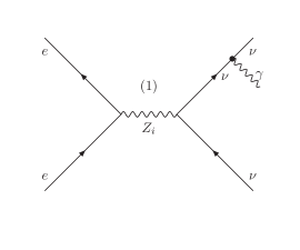
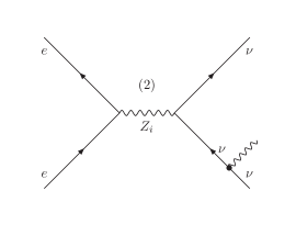
Figure 1: Feynman diagrams contribution to process $e^{+}e^{-}\rightarrow\bar{\nu}\nu\gamma$ in the $SU(4)_{L}\times U(1)_{X}$ model

The decay of $Z_{i}$ to $e^{+}e^{-}$ has the same structure as the decay of Z boson in to $e^{+}e^{-}$. The decay of Z boson in to $e^{+}e^{-}$ is given by PDG .

$$\Gamma_{(Z_{1}\rightarrow e^{+}e^{-})}=\frac{\alpha M_{Z_{i}}}{12}\frac{[g_{V}^{2}(e)+g_{A}^{2}(e)]}{s^{2}_{W}(1-x_{2})}$$ (33)

where $\alpha=\frac{e^{2}}{4\pi}$ is the fine structure constant.

The decay rate of $Z_{i}$ to $e^{+}e^{-}$ can be calculated as:

$$\Gamma_{(Z_{i}\rightarrow e^{+}e^{-})}=\Gamma_{(Z_{1}\rightarrow e^{+}e^{-})}\frac{M_{Z_{i}}}{M_{Z_{1}}}\frac{[g^{2}_{iV}(e)+g^{2}_{iA}(e)]}{[g^{2}_{1V}(e)+g^{2}_{1A}(e)]}\,.$$ (34)

In the followings we will investigate the decay of $Z_{i}\rightarrow\bar{\nu}\nu\gamma$. The Feynman diagrams of this decay is given in Fig.1

$${\cal M}_{1}(\bar{\nu}\nu\gamma) =\epsilon^{\mu}_{\delta}(p)\epsilon^{\beta}_{\lambda}(q)\left[\bar{u}(p_{3})\Gamma^{\mu}\frac{i(k\!\!\!/+m_{\nu})}{(k^{2}-m^{2}_{\nu})}\frac{(-ig)}{2c_{W}}\gamma^{\beta}[g_{iV}(\nu)-g_{iA}(\nu)\gamma_{5}]v(p_{4})\right]$$ (35)

$${\cal M}_{2}(\bar{\nu}\nu\gamma) =\epsilon^{\mu}_{\delta}(p)\epsilon^{\beta}_{\lambda}(q)\left[\bar{u}(p_{3})\frac{(-ig)}{2c_{W}}\gamma^{\beta}[g_{iV}(\nu)-g_{iA}(\nu)\gamma_{5}]\frac{i(k\!\!\!/+m_{\nu})}{(k^{2}-m^{2}_{\nu})}\Gamma^{\mu}v(p_{4})\right]\,,$$ (36)

where

$$\Gamma^{\alpha}=eF_{1}(q^{2})\gamma^{\alpha}+\frac{ie}{2m_{\nu}}F_{2}(q^{2})\sigma^{\alpha\mu}q_{\mu}+eF_{3}(q^{2})\gamma_{5}\sigma^{\alpha\mu}q_{\mu},$$

is the tau-neutrino electromagnetic vertex, $e$ is the charge of the electron, $q^{\mu}$ is the photon momentum and $F_{1,2,3}(q^{2})$ are the electromagnetic form factors of the neutrino, corresponding to charge radius, MM and EDM, respectively, at $q^{2}=0$ R. Escribano , while $\epsilon^{\lambda}_{\alpha}$ is the polarization vector of the photon. $p$ and $k$ stand for the momenta of the Z and neutrino, respectively.

Summing over spin, the square of the scattering amplitude is:

$$\sum_{s}\mid{\cal M}_{1,2}\mid^{2}=\frac{g^{2}}{4\cos^{2}\theta_{W}}(\mu^{2}_{\nu_{\tau}}+d^{2}_{\nu_{\tau}})[(g^{2}_{iV}(\nu)+g^{2}_{iA}(\nu))(s-2\sqrt{s}E_{\gamma})+g^{2}_{iA}(\nu)E^{2}_{\gamma}\sin^{2}\theta_{\gamma}],$$ (37)

The decay rate of gauge boson $Z_{i}\rightarrow\nu\bar{\nu}\gamma$ is therefore calculated as:

$$\Gamma_{(Z_{i}\rightarrow\nu\bar{\nu}\gamma)} = \int\frac{\alpha(\mu_{\nu_{\tau}}^{2}+d_{\nu_{\tau}}^{2})}{64\pi^{2}M_{Z_{i}}x_{W}(1-x_{W})}[(g^{2}_{iV}(\nu)+g^{2}_{iA}(\nu))(s-2\sqrt{s}E_{\gamma})+g^{2}_{iA}(\nu)E^{2}_{\gamma}\sin^{2}\theta_{\gamma}]$$ (38)

$$E_{\gamma}dE_{\gamma}d\cos\theta_{\gamma}\,.$$

Substituting above expression into (32) we have the total cross section of the process $e^{+}e^{-}\rightarrow\bar{\nu}_{\tau}\nu_{\tau}\gamma$:

$$\sigma(e^{+}e^{-}\rightarrow\nu\bar{\nu}\gamma) = \sum_{i=1,2,3}\int E_{\gamma}dE_{\gamma}d\cos\theta_{\gamma}\frac{\alpha^{2}(\mu_{\nu_{\tau}}^{2}+d_{\nu_{\tau}}^{2})}{192\pi}\frac{[g^{2}_{iV}(e)+g^{2}_{iA}(e)]}{x^{2}_{W}(1-x_{W})^{2}}$$ (39)

$$\times\frac{[(g^{2}_{iV}(\nu)+g^{2}_{iA}(\nu))(s-2\sqrt{s}E_{\gamma})+g^{2}_{iA}(\nu)E^{2}_{\gamma}\sin^{2}\theta_{\gamma}]}{(s-M^{2}_{Z_{i}})^{2}+M^{2}_{Z_{i}}\Gamma^{2}_{Z_{i}}}\,.$$

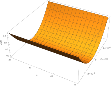
Figure 2: The total cross section for $e^{+}e^{-}\rightarrow\bar{\nu}\nu\gamma$ as the function of the ration of $\frac{m_{Z^{\prime}}}{m_{Z}}$ and $\mu_{\nu_{\tau}}$

IV Results

In investigating numerically the cross section, the photon angle and energy will be cut to avoid the divergence of the integral when integrating over important intervals. We integrate over $\theta_{\gamma}$ from $44.5^{o}$ to $135.5^{o}$ and $E_{\gamma}$ from 15 GeV to 100 GeV. The following numerical values are used: sin${}^{2}\theta_{W}=0.23126\pm 0.00022$, $M_{Z}=91.1876\pm 0.0021GeV$, $\Gamma_{Z}=2.4952\pm 0.0023GeV$. We approximate the mass of the two new neutral bosons are of the same order $(M_{Z_{2}}\approx M_{Z_{3}})$ therefore their decay rate can be approximate to have the same order $\Gamma_{Z_{2}}\approx\Gamma_{Z_{3}}$. The decay width of the $Z_{2}$, $Z_{3}$ bosons are approximate as: $\Gamma_{Z_{2,3}}=2\Gamma_{Z_{1}}$ Z23decayrate and the mass of $Z_{2}$, $Z_{3}$ bosons can be approximate as $M_{Z_{2,3}}=x_{r}M_{Z_{1}}$ where $x_{r}=\frac{M_{Z_{2}}}{M_{Z_{1}}}$. The mass limit of the new neural gauge boson is $M_{Z^{\prime}}<5$ TeV Z'masslimit equivalent to $x_{r}\approx 50$. We obtain the total cross section $\sigma_{Tot}=\sigma_{Tot}(\mu_{\nu_{\tau}},d_{\nu_{\tau}},\sqrt{S},x_{r})$. We will evaluate the total cross section as a function of the parameters of the model, $x_{r}$, which is the ratio of the symmetry breaking scale of the group $SU(4)_{L}$ and the vacuum expectation value of the $SU(2)_{L}$ and the center of mass energy. Using the approximation that the total number events N $\approx\sigma_{Tot}\cal{L}$ Nevents where $N=N_{B}+\sqrt{N_{B}}$ B is the total number of $e^{+}e^{−}\rightarrow\bar{\nu_{\tau}}\nu_{\tau}\gamma$ events expected at $1\sigma,2\sigma,3\sigma$ we can set the bounds of the tau neutrino magnetic dipole moments with $d_{\nu_{\tau}}=0$ for different integrated luminosity $\cal{L}$. This analysis can be used to obtain the bound on the tau neutrino electric dipole moment with $\nu_{\tau}=0$

${\cal L}=500,\hskip 2.27621pt1000,\hskip 2.27621pt2000\hskip 2.27621ptfb^{-1}$
$\sqrt{S}=1.0\hskip 2.27621ptTeV;x_{r}=20$
C.L.	$|\mu_{\nu_{\tau}}(\mu_{B})|$	$|d_{\nu_{\tau}}(e.cm)|$
1$\sigma$	$(0.35,0.25,0.17)\times 10^{-10}$	$(1.03,0.73,0.51)\times 10^{-19}$
2$\sigma$	$(0.40,0.28,0.20)\times 10^{-10}$	$(1.18,0.84,0.59)\times 10^{-19}$
3$\sigma$	$(0.41,0.29,0.20)\times 10^{-10}$	$(1.22,0.86,0.61)\times 10^{-19}$
$\sqrt{S}=2.0\hskip 2.27621ptTeV;x_{r}=35$
C.L.	$|\mu_{\nu_{\tau}}(\mu_{B})|$	$|d_{\nu_{\tau}}(e.cm)|$
1$\sigma$	$(0.51,0.36,0.25)\times 10^{-10}$	$(2.0,1.43,1.01)\times 10^{-19}$
2$\sigma$	$(0.58,0.41,0.29)\times 10^{-10}$	$(2.34,1.65,1.17)\times 10^{-19}$
3$\sigma$	$(0.60,0.42,0.30)\times 10^{-10}$	$(2.4,1.70,1.20)\times 10^{-19}$
$\sqrt{S}=3.0\hskip 2.27621ptTeV;x_{r}=50$
C.L.	$|\mu_{\nu_{\tau}}(\mu_{B})|$	$|d_{\nu_{\tau}}(e.cm)|$
1$\sigma$	$(1.02,0.72,0.51)\times 10^{-10}$	$(3.0,2.12,1.50)\times 10^{-19}$
2$\sigma$	$(1.18,0.83,0.59)\times 10^{-10}$	$(3.46,2.49,1.73)\times 10^{-19}$
3$\sigma$	$(1.21,0.85,0.60)\times 10^{-10}$	$(3.55,2.51,1.78)\times 10^{-19}$

Table 2: Bounds on the $\mu_{\nu_{\tau}}$ magnetic moment and $d_{\nu_{\tau}}$ electric dipole moment for $\sqrt{S}=1,2,3$ TeV and $\cal{L}$=500, 1000, 2000 fb^-1 at 1$\sigma$, 2$\sigma$, 3$\sigma$

We present the bounds obtained on the $\mu_{\nu_{\tau}}$ magnetic moment and $d_{\nu_{\tau}}$ electric dipole moment in Table II to demonstrate the order of magnitude. From Table II we can see that our result is better than those given in literature T.M.Gould ; CLIC ; M. Acciarri ; R. Escribano ; tauneu-mmboud1 ; tauneu-mmboud2 ; tauneu-mmboud3 ; tauneu-mmboud4 and approach the limit by Borexino experiment Borexino .

In the case of the electric dipole moment our result show that these bounds are of order $10^{-19}$-$10^{-20}$ for the 95% C.L. sensitivity limits at 1000 - 3000 GeV center of mass energies and integrated luminosities of 2000 $fb^{−1}$. These bounds are improved by 2-3 orders of magnitude than those reported in the literature tauneu-mmboud1 ; tauneu-mmboud2 ; tauneu-mmboud5 ; tauneu-mmboud6

In Fig. 2 we evaluate the cross-section of the process $e^{+}e^{-}\rightarrow\bar{\nu}\nu\gamma$ as the function of the ration of $\frac{m_{Z^{\prime}}}{m_{Z}}$ and $\mu_{\nu_{\tau}}$ with the value of $\sqrt{S}=500$GeV. The value of the magnetic moment investigated is up to the current value of the L3 experiment $\mu_{\nu_{\tau}}=3.3\times 10^{-6}(\mu_{B})$. Our result is of the same order with previous result tauneu-mmboud5

In summary, we conclude that the estimated limits for the tau-neutrino magnetic and electric dipole moments in the context of a $SU(4)_{L}\times U(1)_{X}$ model compare favorably with the limits obtained by the L3 Collaboration and complement previous studies on the dipole moments.

References

(1) SNO Collab., Q. R. Ahmad et al., Phys. Rev. Lett. 87 (2001) 071301.
(2)
SK Collab., Y. Fukuda, et al., Phys. Rev. Lett. 81 (1998) 1562; 86 (2001) 5651;
86 (2001) 5656.
(3)
W. J. Marciano and A. I. Sanda, Phys. Lett. B 67, 303 (1977); B. W. Lee and R. E. Shrock, Phys. Rev. D 16, 1444 (1977).
(4)
J. Bernstein, M. Ruderman, and G. Feinberg, Phys. Rev. 132, 1227 (1963).
(6) O.G. Miranda et al., Nucl. Phys. B 595 (2001) 360;
O.G. Miranda et al., Phys. Lett. B 521 (2001) 299.
(7)K. Fujikawa and R. Shrock, Phys. Rev. Lett. 45 (1980) 963
(8)C. Arpesella et al. [The Borexino Collaboration], Borexino Data,” Phys. Rev. Lett. 101 (2008)
091302. [arXiv:0805.3843 [astro-ph]]; H. T. Wong et al. [TEXONO Collaboration], Phys. Rev. D 75, 012001 (2007) [hepex/0605006]; A. G. Beda, V. B. Brudanin, V. G. Egorov, D. V. Medvedev, V. S. Pogosov, M. V. Shirchenko
and A. S. Starostin, Adv. High Energy Phys. 2012, 350150 (2012); G. G. Raffelt, Phys. Rev. Lett. 64 (1990) 2856.
(9) M. Fukugita and T. Yanagida, Physics of Neutrinos and
Applications to Astrophysics, (Springer, Berlin, 2003).
(10) A. Cisneros, Astrophys. Space Sci.10, 87 (1971).
(11) C. Arpesella, et al., [Borexino Collaboration], Phys. Rev. Lett. 101, 091302 (2008).
(12) R. Schwinhorst, et al., [DONUT Collaboration], Phys. Lett. B 513, 23 (2001).
(13) A. M. Cooper-Sarkar, et al., [WA66 Collaboration], Phys. Lett. B 280, 153 (1992).
(14) M. Acciarri et al., [ L3 Collaboration], Phys. Lett. B 412, 201 (1997).
(15)K. Nakamura et al., (Particle Data Group), J. Phys. G 37, 075021 (2010).
; Rick S. Gupta and James D. Wells, arXiv: 1110.0824 [hep-ph]; G. L. Bayatian et al., (CMS Collaboration), J. Phys. G 34, 995 (2007).
(16) T. M. Gould and I. Z. Rothstein, Phys. Lett.B 333, 545 (1994).
(17) H. Grotch and R. Robinet, Z. Phys.C 39, 553 (1988).
(18) G. Senjanovic, Nucl. Phys.B 153, 334 (1979).
(19) G. Senjanovic and R. N. Mohapatra, Phys. Rev.D 12, 1502 (1975).
(20) U. Baur et al., Phys. Rev.D 35, 297 (1987).
(21)F. Pisano and V. Pleitez, Phys. Rev. D 46, 410 (1992);
J. C. Montero, F. Pisano and V. Pleitez, Phys. Rev. D 47, 2918 (1993);
[14] H. N. Long, Phys. Rev. D 53, 437 (1996).
(22) M. B. Voloshin, Sov. J. Nucl. Phys. 48, 512 (1988).
(23)R. Foot, H. N. Long, and T. A. Tran, Phys. Rev. D 50, R34 (1994), [arXiv: hep-ph/9402243]; F. Pisano and V. Pleitez, Phys. Rev. D 51, 3865 (1995); A. Palcu, Phys. Rev. D 85, 113010 (2012), arXiv:1111.6262
(24)H. N. Long, L. T. Hue, and D. V. Loi, Phys. Rev. D 94, 015007 (2016), [arXiv:1605.07835(hep-ph)], and references therein.
(25) N. A. Ky, H. N. Long, and D. V. Soa,
Phys. Lett.B 486, (2000) 140, [arXiv: hep-ph/0007010].
(26) T. Abe et al., “Linear collider physics resource book for snowmass 2001—part 3: studies of exotic and standard model physics,” http://arxiv.org/abs/hep-ex/0106057.
(27) E. Accomando, A. Aranda, E. Ateser et al., “Physics at the CLIC Multi-TeV linear collider,” http://arxiv.org/abs/hep-ph/0412251v1
(28) C. Patrignani et al. (Particle Data Group), Chin. Phys. C 40, 100001 (2016)
(29)R. Escribano and E. Mass´o, Phys. Lett. B 395, 369 (1997);
(30) P. Vogel and J. Engel, Phys. Rev. D 39, 3378 (1989).
(31)F. Abe et al., CDF Coll., Phys. Rev. Lett. 68, 1463 (1992)
(32)G.L. Bayatian et al. [CMS Collab.], J. Phys. G 34, 995
(2007).
(33)M. Acciarri, O. Adriani, M. Aguilar-Benitez et al., Physics Letters B 412, 201 (1997)
(34)
A. Guti´errez-Rodr´ıguez, et al., Phys. Rev. D 74, 053002 (2006).
(35)
A. Guti´errez-Rodr´ıguez, et al., Phys. Rev. D 69, 073008 (2004)
(36)
A. Guti´errez-Rodr´ıguez, et al., Phys. Rev. D 58, 117302 (1998)
(37)
P. Abreu, et al., [DELPHI Collaboration], Z. Phys. C 74, 577 (1997).
(38)A. Gutierrez-Rodriguez, et al., Eur. Phys. J. C 71 (2011) 1819
(39)
A. Gutiérrez-Rodríguez, M. Koksal, and A. A. Billur
Phys. Rev. D 91, 093008 (2015)